3d finite difference time-domain modeling of acoustic wave
TRANSCRIPT

1
3D Finite Difference Time-Domain Modeling of Acoustic Wave Propagation based on Domain
Decomposition
UMR Géosciences AzurCNRS-IRD-UNSA-OCA
Villefranche-sur-merSupervised by: Dr. Stéphane Operto
Jade Rachele S. GarciaJuly 16, 2009

2
Outline
1. Introduction
2. Scope and Aim of the Work
3. The Forward Problem: Seismic Wave Modeling
4. Parallel Implementation
5. Numerical Results
6. Conclusion

3
Introduction

4
Seismic Exploration
Seismic Exploration – the search for subsurface deposits of crude oil, natural gas and minerals
Objective: to form a model of the subsurface
The basic processes in seismic exploration: Controlled sources emit elastic waves which
propagate in the subsurface Record the wavefield propagated by the different
layers Process the seismic data to produce some models
of the subsurface

5
Full Waveform Inversion
Full Waveform Inversion – a data fitting procedure that utilizes the full information contained in the seismic data to produce high resolution models of the subsurface
Two main ingredients: the forward problemand the inverse problem

6
Full Waveform Inversion
where
The Forward Problem
The Inverse Problem
Model Data

7
Scope and Aim of the Work
The focus of this paper : implement and validate the 3D parallelfinite-difference time-domain code for acoustic wave modeling (part of the Forward Problem)
Motivations: Build a forward modeling engine in the time domain to perform
3D acoustic full-waveform inversion in the frequency domain. Design an acoustic code with judicious stencil that will be easily
extended to the 3D elastic case. The 3D elastic code will be used:
1. as forward modeling engine to perform 3D elastic full-waveform inversion
2. to perform cross-validation with a Discontinuous Galerkin finite-element method developed by V. Etienne at Geosciences Azur
3. Perform wave modeling for other kinds of application such as seismic hazards assessment.

8
The Forward Problem: Seismic Wave Propagation Modeling

9
The Acoustic Wave Equation: The Earth as a Fluid
The acoustic wave equation describes sound waves in a liquid or gas.
Acoustic wave equation: not very accurate for modeling wave propagation in solids but is relatively simple to solve
Acoustic wave: essentially a pressure change. Since, fluids exhibit fewer restraints to deformation, the restoring force responsible for wave propagation is simply due to pressure change

10
Velocity-Stress Formulation of the Acoustic Wave Equation
Initial conditions: P and V are zero at t=0
Boundary conditions: Absorbing boundary conditions and free surface boundary condition
11
The Finite Difference Discretization of the 3D Acoustic Wave Equation
12
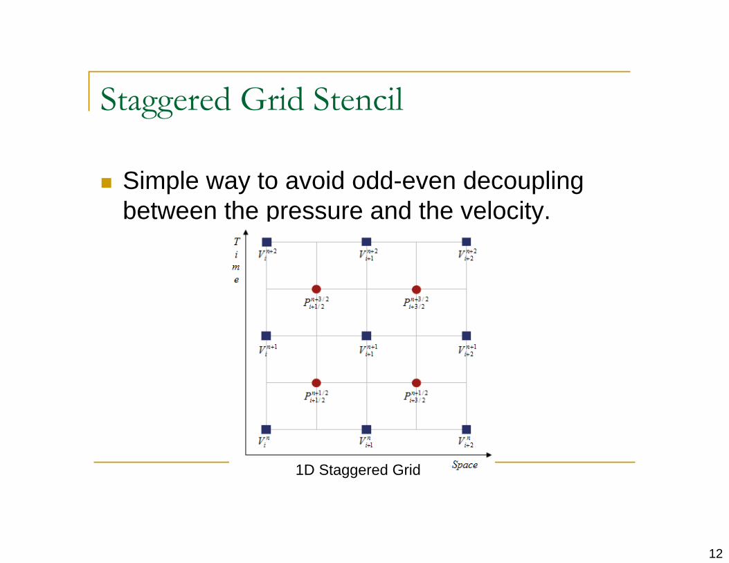
Staggered Grid Stencil
Simple way to avoid odd-even decoupling between the pressure and the velocity.
1D Staggered Grid
13
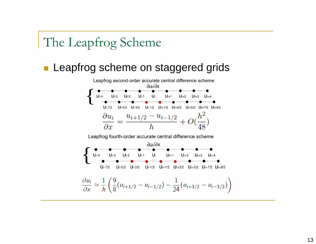
The Leapfrog Scheme
Leapfrog scheme on staggered grids

14
The Discretized 3D Acoustic Wave Equation Using the 2nd order discretization for time and 4th order
discretization for space in a staggered grid leads to:

15
Numerical Dispersion and Stability

16
Numerical Dispersion
- variation of the numerical phase velocity as a function of frequency
Occurs if: Grid spacing is large Wavelength of the source is too short compared
with the size of the grid

17
Numerical Dispersion
For a Ricker wavelet, the rule of the thumb given below is an effective criterion for nondispersive propagation
n is the number of gridpoints per wavelength. For a 4th order accurate scheme, it has been established to be 5-8 gridpoints per wavelength.
nx

18
Numerical Stability
Numerical instability – an undesirable property that may occur in explicit time-marching schemes, when the computed result spuriously increases without limit in time
A stability condition for the time step is the Courant-Friedrichs-Levy (CFL) condition. For the scheme used here,
48.0 where,max
c
xt

19
An Illustration through the 1D Case

20
The 1D Scalar Wave Equation in Homogeneous Medium To illustrate the numerical analysis involved in finite
difference discretization, we start with the simplest case, the one-dimensional homogeneous scalar wave equation
A fully explicit second-order accurate finite difference approximation of the wave equation
21
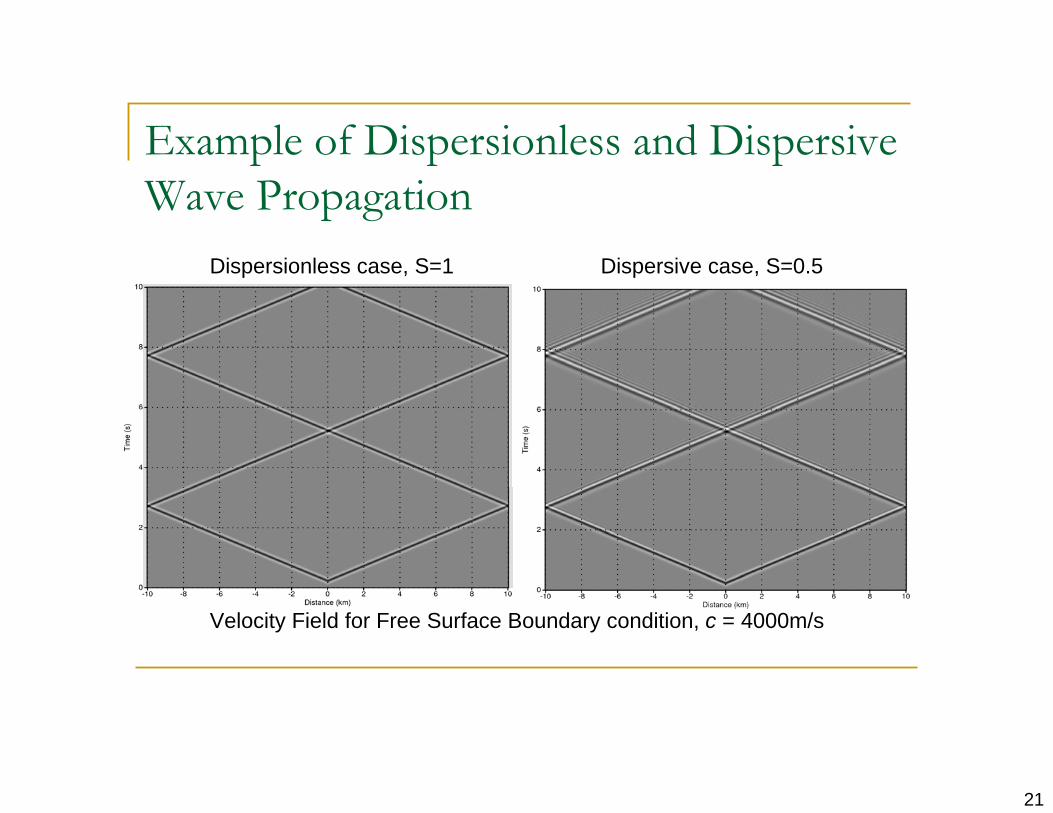
Example of Dispersionless and Dispersive Wave Propagation
Velocity Field for Free Surface Boundary condition, c = 4000m/s
Dispersionless case, S=1 Dispersive case, S=0.5
22
Simulation of an Unbounded Medium in 1D Radiation condition
Sponge boundary condition

23
Radiation Condition

24
Radiation Condition
Simulation in a two-layer medium c1=2000 m/sc2=4000 m/s – S=1 in the high-velocity layer
Simulation in homogeneous medium c=4000 m/s (dispersionless – S=1)

25
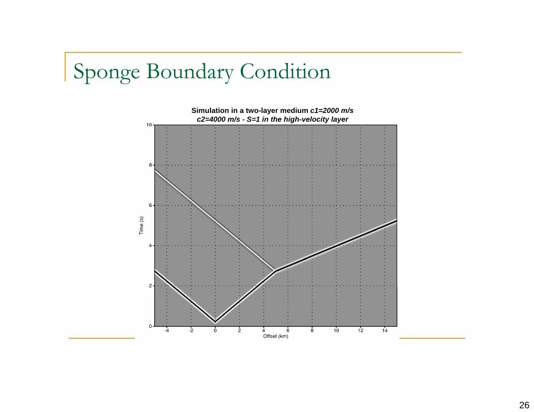
Sponge Boundary Condition
26
Sponge Boundary ConditionSimulation in a two-layer medium c1=2000 m/s
c2=4000 m/s - S=1 in the high-velocity layer
27
Parallel Implementation

28
Methodology
A parallel version of the general algorithm based on the principle of domain decomposition for structured meshes is as follows:
Decompose the mesh into subdomains and assign each subdomain to a process
Determine the neighbors of each subdomain Iterate time Exchange messages among interfaces calculate
29
Subroutines
SUBROUTINE init
SUBROUTINE voisinage
SUBROUTINE typage
SUBROUTINE communication

30
SUBROUTINE init
This procedure init executes the decomposition of the original domain into subdomains and the initialization of MPI
31
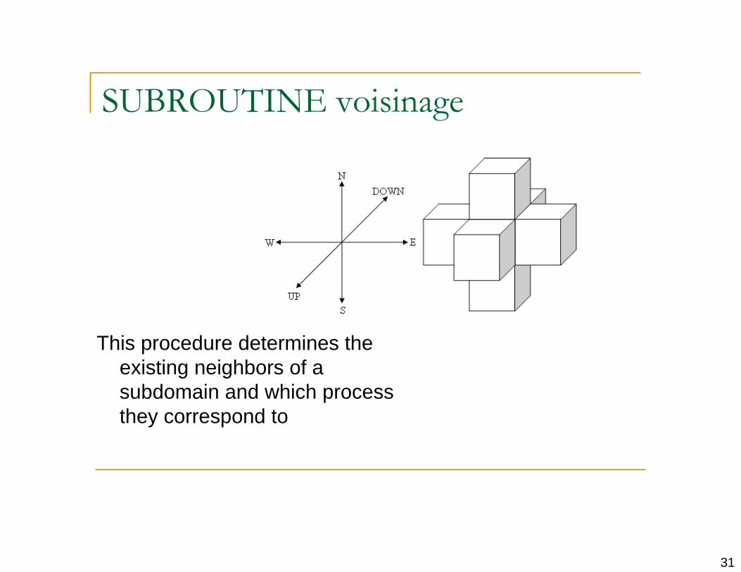
SUBROUTINE voisinage
This procedure determines the existing neighbors of a subdomain and which process they correspond to

32
SUBROUTINE typage
This procedure defines the data blocks to be send in sending and receiving messages

33
SUBROUTINE typage
To pass data to and from the overlaps of subdomains, data types foreach type of face are defined by using the following MPI functions:
MPI TYPE VECTOR(number of blocks, number of elements in each block,number of elements between the start of each block, old type, new type)-- allows replication of a datatype into locations that consist of equally spaced blocks.
MPI TYPE HVECTOR-- almost the same as MPI TYPE VECTOR except that the stride (3rd parameter) between the start of each block is in bytes instead of the number of elements

34
SUBROUTINE communication
This procedure is done within the loop in time
Its purpose is to send data blocks from the subdomain to the corresponding neighboring areas and to receive the same points in the relevant fields
Use MPI_SENDRECV(initial address of sending, number of elements to be sent, type of elements to send, destination, initial address of reception, number of
elements to receive, source)

35
SUBROUTINE communication
For each subdomain, a three-dimensional array (to be called x) is allocated as:
x(-1:n1loc+2,-1:n2loc+2,-1:n3loc+2)
Below is a table that summarizes the communication procedure
36
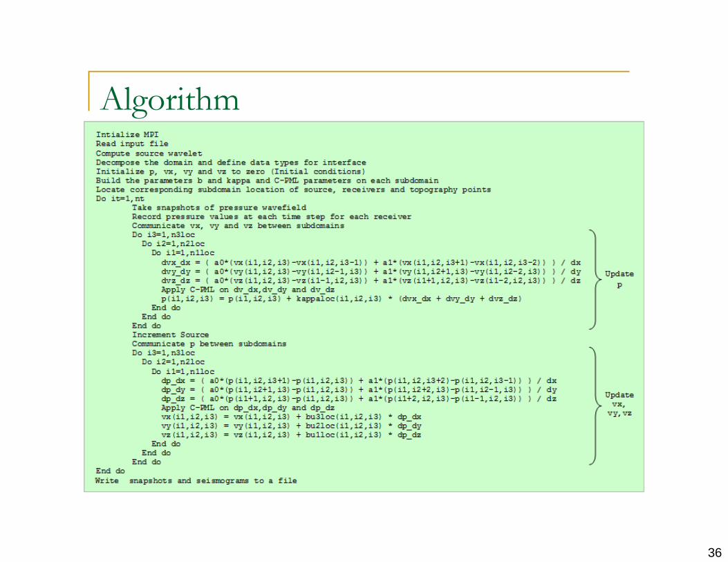
Algorithm
37
Numerical Results

38
Comparison with Analytical Solution in Homogeneous Medium
39
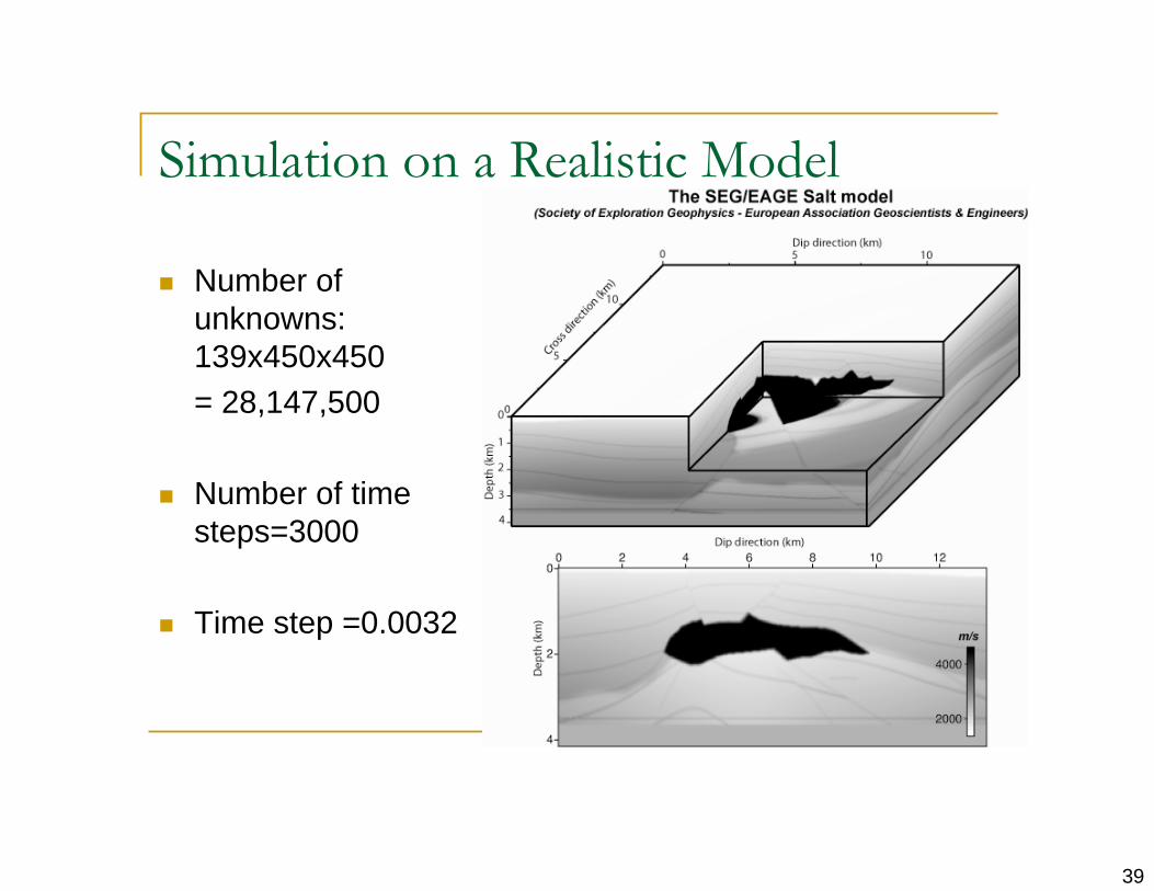
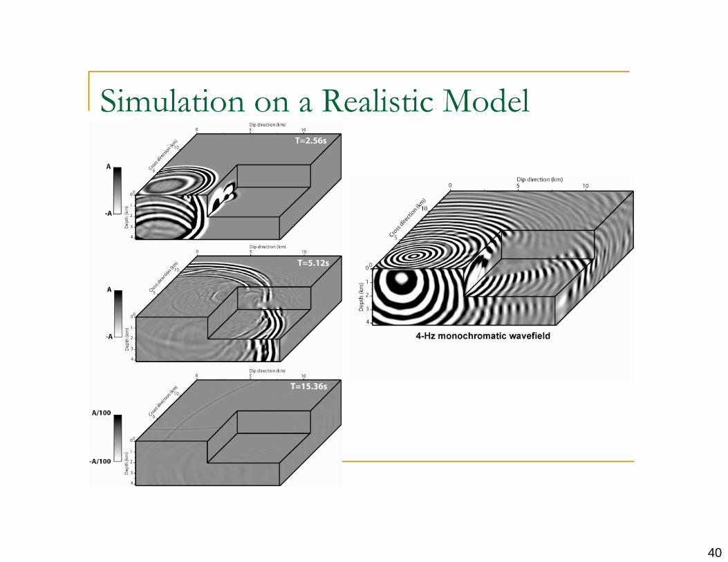
Simulation on a Realistic Model
Number of unknowns: 139x450x450 = 28,147,500
Number of time steps=3000
Time step =0.0032
40
Simulation on a Realistic Model
41
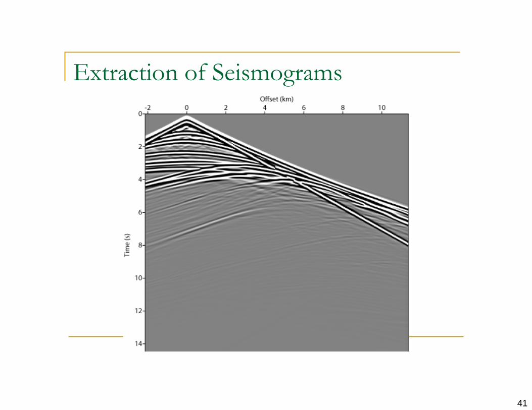
Extraction of Seismograms
42
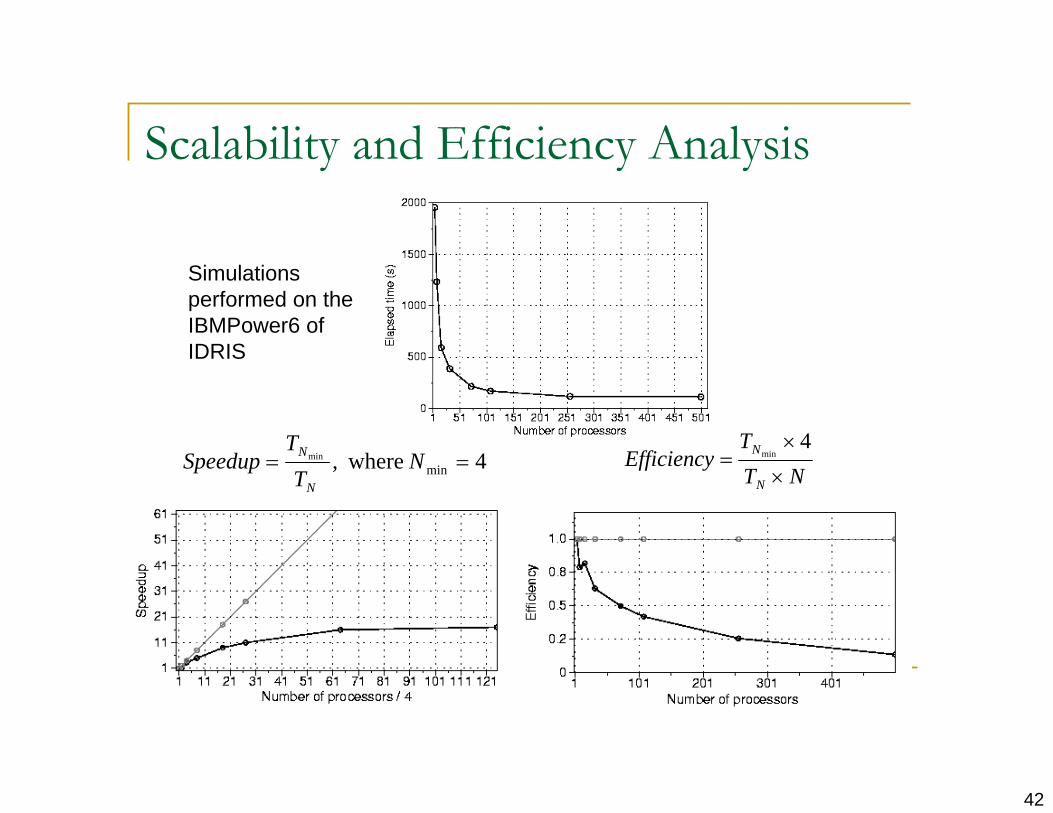
Scalability and Efficiency Analysis
4 where, minmin N
TT
SpeedupN
N
NTT
EfficiencyN
N
4min
Simulations performed on the IBMPower6 of IDRIS

43
Scalability and Efficiency
44
Conclusions
45
Conclusion
Validate the accuracy of the FDTD code Validate the efficiency of the absorbing boundary
condition: C-PML Validate the computational efficiency of the code on
realistic example computed on a large-scale distributed memory platform
Conclusion: we have a modeling engine which is ready to be implemented in a 3D acoustic Full Waveform Inversion code

46
Perspectives
Extension to the elastic through rotated stencil
Implementation of the FDTD code in FWI which can be viewed in two levels of parallelism: Perform modeling in sequential and distribute the
sources (rhs) over processors Classical domain decomposition of the number of
sources are much less than the number of processors
47
Thank you for listening!
Special thanks to Prof. Operto.