3D Horizon/Fault Interpretation ExerciseUsing Seismic Micro-Technology’s PC based 2d/3dPAK Seismic

Interpretation Software

Prepared by Tom Wilson, Appalachian Region Resource Center, Petroleum Technology Transfer Councilbased on procedural steps developed by Mike Enomoto of Seismic MicroTechnology Inc. Houston, TX.

Fault/Horizon Interpretation UsingSeismic Micro-Technology’s 2d/3dPAK

This manual is based on a set of procedural steps provided by Mike Enomoto ofSeismic Micro-Technology, Inc. for the 2d/3dPAK Users Group meeting hosted byAppalachian Region Resource Center on June 23rd of 1997.

NOTE: Left clicking the mouse is used to start, continue and end anactivity. Right clicking is ONLY used for displaying the pop-upmenu.

This fault/horizon interpretation exercise was presented at the June23rd 1997 Users Group meeting hosted by the Appalachian RegionPetroleum Technology Resource Council’s Resource Center on thecampus of West Virginia University. Questions about the steps andprocedures listed below can be directed to SMT technical staff intheir Houston office at (713) 464 6188.

Data for the following exercise was provided by Seismic Micro-Technology. In this exercise, the B46 formation top is selected fromany well and then tied around to the remaining wells. The entire 3Dgrid is interpreted. It is recommended that major faults beinterpreted at the outset, since this will prevent autopicking of selectreflection events across fault planes.

Procedures:When you open a project under Kingdom, the basic windows layoutwill contain a 3D basemap (right) and project tree (left) (Figure 1).

Figure 1: Basic window layout showing project tree and 3D gridbasemap.

1. Left click on the 3D grid (Figure 1) to activate it. In thisexample, position the cursor on line 110. Right click and selectDisplay Line 110. The seismic line will now appear as shownbelow in Figure 2.

Figure 2: Display of 3D line 110.

2. If you prefer another colorbar, left click on View and Colors.Click on File and Open and select a different colorbar. In mostcases, the name of the colorbar describes the colors and thenumber of colors in the colorbar. For example, the defaultcolorbar, brwbl50.clm, is a blue-white-brown colorbar with 50colors. Close the color editor once you are satisfied with acolorbar.

3. If you are accustomed to wiggle trace overlay, left click onView and Type of Plot and select Wiggle Variable Area. Youmay need to change the scale in order to display properly. Thevariable area wiggle trace display will appear as shown below(Figure 3). Note the other display formats for future reference.

Figure 3: Variable area wiggle trace display format of Line 110.

4. To change the display scales, left click on View and SetDisplay Scales or click on the scale bar at the top of the seismicline display window. Try 5 traces per inch and 10 inches persecond to provide a closeup (Figure 4) view of waveformcharacter in the vicinity of the well shown above (Figure 3).Use the scroll bars to position yourself within the line.

Figure 4: Closeup view obtained using 5 traces per inch and 10inches/seconds.

5. You can orient yourself to geographical directions by movingthe cursor on the seismic window (Figures 3 or 4) and watch thecursor movement on the map. If the direction is backwards hitthe R key on the keyboard to reverse the line direction.

6. The colorbar may or may not be displayed on the seismicwindow. To display colorbar, left click on View and Toolbarsand then Color Bar. A check indicates “on”.

7, On the seismic line, several faults are prominently displayed.Many are easily correlatable, others are not. Now would be agood time to assign a name to at least two of the major faults,the down to the south and the antithetic. The others may bepicked as assigned or unassigned. To assign the faults, rightclick on the seismic window and select Fault Management.From there, select the Create tab and enter a name and color forthe antithetic fault. Left click on Apply. Enter a name andcolor for the major fault and then either OK or Apply. Createnew faults if desired, You're now in the fault picking mode withthe last created fault active.

8. Display the fault toolbar to allow for quicker selection of thefaults you wish to pick. To do this left click on View andToolbars and then Faults. All the displayed faults are present,including Unassigned. Hot keys are available: “d” is digitize,“a” is assign, and 's' is de-assign.

9. To start picking your fault, left click on the one of the faultnames. To begin digitizing hit the D key and then left click onthe fault break that courses through the seismic data. A rubberband should appear as you go from point to point. Continue leftclicking on the break until you either need to scroll vertically orhorizontally. At this point, double click to end the segment.Use the scroll bar to move the display so that more of the faultis visible. The fault should have square dots representing thedigitized points. If so, left click on the last point and thencontinue until you can no longer pick this fault. Double click toend. If no square dots are present, the fault is not active andsimply requires a left click anywhere on the fault to activate.

If you enter a point you don’t like, you can back up or deletethe last by hitting the Esc key

10. Left click on the other fault displayed in the Faults menu toactivate it and then hit the “D" key to begin digitization. Beginpicking the second fault. If you choose to pick some of the other

faults on the Faults Toolbar, simply activate the appropriatenamed or unassigned fault, hit the “D” key and start picking.The two faults you just picked should appear as shown in themontage below (Figure 5). The number of points used todigitize the fault will vary from interpreter to interpreter.

Figure 5: Project tree (back left) and basemap (right) lie in thebackground behind seismic Line 110 (right) and the Faultsmenu (small window at left). Faults just digitized on thenorthern end of the line appear as shown above.

11. If you want to edit some of your picks, the fault is active solong as the square dots are present. Note that the black fault inthe above display is currently active. To move points, activatethe fault and then left click and hold on the digitized fault point.As you move the mouse, the digitized point will also move. Ifyou move more than one point you may have to use the Esc keyto undo the rubber band.

12. If you would like to move the entire fault line, first activatethe fault and then hold the Ctrl key and then left click and holdon any part of the fault line. Move the line to wherever you likeand then release the mouse button and Ctrl key.

13. To delete a fault segment, make it active and then hit thedelete key on your keyboard.

14. To add points, left click on an existing point, add theappropriate intervening points, and double click on anotherexisting point.

15. To remove consecutive points, left click on an existingpoint, skip the 'bad' points and double click on an existing point.

16. If you'd like to change faults on the display. left click onthe fault to activate. or select from the Faults Menu. If the newfault has no existing digital points, you must hit 'D' on either thekeyboard or Faults Menu. DO NOT HIT THE "D" KEY IFEDITING A FAULT.

17. To assign an unnamed fault, activate the fault name,activate the unassigned fault line and then hit the A key.

18. To de-assign a named fault activate the fault line and thenhit the S key.

19. Once the faults have been picked on this line, you can beginpicking the faults on a grid of lines extending through the entire3D data base. To set the grid spacing, left click on Line and SetLine Skip Increment. Set the increment to 20 and then OK.Now whenever the right arrow on the keyboard is hit. the linedisplayed will increase by 20. If the left arrow is hit. the displaywill decrement by 20. If a cross line is displayed, the up anddown arrow keys will work likewise.

20. Go to line 130 and pick the faults.

21. Once an assigned fault has been picked on at least twolines, a fault surface is automatically created. To view faultsurfaces in map view go to the Project Tree and double click onthe appropriate fault icon. This makes that fault surface theactive subset and opens a new map window where the fault maybe displayed as either a fault plane or lines. To toggle fromplanes to lines, go to View, Fault Display Mode and selecteither Fault Surface or Fault Segment.

Map and line views are shown in the montage below (Figure 6).

Figure 6: The large synthetic fault dipping to the south isdisplayed in both line and map views. Color coded two-waytravel times appear in the color bar at right.

LINES

MAP

22. Display the fault surface in seismic view so that anymiscorrelation can be quickly seen. To do this, go to a seismicwindow and right click, go to Fault Management, and Display.Verify that Both is selected for Display Type. If “Both” isselected, two lines are visible in seismic view, the straight lineconnecting the digitized points and the interpolated faultsurface.

23. Complete fault picking: Continue over to the east end of thesurvey to Line 145. Then return to line 90 and continue to thewest. To go to line 90, left click on Line and then Select or leftclick on the arrow button in the seismic display window whichbrings up the same window. Type in 90 and be sure the linebutton is on and that the 3d survey is displayed. Hit OK. If youwould like to view the faults in strike direction or on anarbitrary line, right click on the desired cross line in the basemap window and then display. To display line with anarbitrary orientation through the survey, right click on a mapwindow, select Digitize Arbitrary Line, left click on the startingpoint, continue left clicking on each bend in the line and thendouble click to end.

Note: To bring up a fresh basemap click on Window and NewMap Display.

At this point, your fault surfaces will be correlated across theentire survey area. The north-dipping fault surface, for example,will appear as shown below (Figure 7).

24. Continue picking faults, in the western direction.

You can edit interpolated fault picks by first selecting thedesired fault as the active fault in the Fault ManagementWindow, and then hitting the D key to digitize. If you wish tocorrect a portion of the interpolated picks simply begin pickingpoints through the desired region. Double click to completedigitization. Your picks will replace the interpolated picks.

If a fault has been extended too far, you can delete a portion ofthe interpolated fault line by digitizing the extended portion, anddouble clicking to replace the interpolated line with your picks.Then click on the bad pick and drag the rubber band to the firstgood pick and double click. All points beyond the last pick willbe deleted.

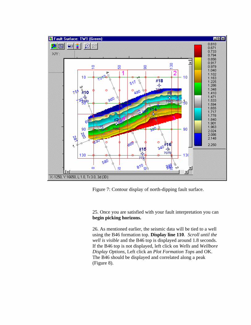
Figure 7: Contour display of north-dipping fault surface.

25. Once you are satisfied with your fault interpretation you canbegin picking horizons.

26. As mentioned earlier, the seismic data will be tied to a wellusing the B46 formation top. Display line 110. Scroll until thewell is visible and the B46 top is displayed around 1.8 seconds.If the B46 top is not displayed, left click on Wells and WellboreDisplay Options, Left click an Plot Formation Tops and OK.The B46 should be displayed and correlated along a peak(Figure 8).

Figure 8: Horizon B46 tied to well on Line 110.

27. Horizons are created in much the same way as faults.Anywhere on the seismic line, right click and select HorizonManagement. Select the Create tab and then enter B46 for thehorizon name and then select a color. Hit OK. The B46horizon is now active.

28. Display the horizon in map view by double clicking on theicon next to the B46 Horizon. Since no picks have been made,no horizon is visible.

29. Horizon Picking: Right click on a seismic line and selectPicking Parameters. Make sure that Stop at Displayed FaultSurface Intersections is enabled. This feature, when enabled,works with the Autopick-2D Hunt mode. Picking will stopeither whenever data goes away or the horizon encounters afault surface.

30. Display the Horizon Toolbar by left clicking on View,Toolbars, and Horizon bar. Note that the active horizon ishighlighted in the toolbar. Hot keys are available, M = manual

picking. F = Fill made, H = 2d Hunt. P = Erase. P = Peak, andT = Trough. Hot keys are not available for zero crossings.

31. Note the shape of the cursor and the status bar. The cursor isnow a '+' with either a E, M, F, or H next to it. Change thepicking mode to either F or H, and change the phase to peak.Pick the event as far as you can, jump the fault if desired. Notethat the map display is updated immediately after picking.

32. Once the inline has been picked, place the cursor oncrossline 70 on the seismic display, right click and display theline. A small tick mark is visible where the two lines intersect.You may also see a vertical red line. This red line is a lineoverlay and can be disabled by left clicking on View andselecting Line Overlays. A check mark indicates 'on'. If youchose the Hunt mode, left click once on the tick mark and theentire horizon between fault segments is completed.. Incrementthrough your data using the arrow keys and continue pickingthis horizon, You should end up with picked grid of lines for theB46 horizon (Figure 9)

Figure 9: Horizon picks are shown on the grid of in-lines andcross lines. Travel times are color coded. Fault intersections arecorrelated through the area.

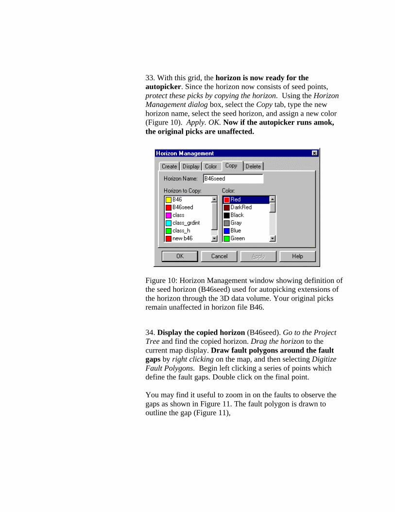
33. With this grid, the horizon is now ready for theautopicker. Since the horizon now consists of seed points,protect these picks by copying the horizon. Using the HorizonManagement dialog box, select the Copy tab, type the newhorizon name, select the seed horizon, and assign a new color(Figure 10). Apply. OK. Now if the autopicker runs amok,the original picks are unaffected.

Figure 10: Horizon Management window showing definition ofthe seed horizon (B46seed) used for autopicking extensions ofthe horizon through the 3D data volume. Your original picksremain unaffected in horizon file B46.

34. Display the copied horizon (B46seed). Go to the ProjectTree and find the copied horizon. Drag the horizon to thecurrent map display. Draw fault polygons around the faultgaps by right clicking on the map, and then selecting DigitizeFault Polygons. Begin left clicking a series of points whichdefine the fault gaps. Double click on the final point.

You may find it useful to zoom in on the faults to observe thegaps as shown in Figure 11. The fault polygon is drawn tooutline the gap (Figure 11),

Figure 11: Fault gaps in horizon B46 appear in closeup view ofthe basemap.

It may help to zoom in and draw polygons around visablesegments in closeup view. Double click to close the polygonsurrounding a restricted segment of the total fault. Then use theslide bars to reposition your viewing area farther along the fault.Continue digitizing the polygon beginning at the end of theprevious polygon. When the rubber band is returned to theadjoining point on the opposing side of the fault, double clickon that point. One continuous polygon will appear. Your faultpolygons may appear as shown in Figure 12 below.

Figure 12: Closeup view of fault polygons drawn around thefault gaps.

35. Left click on Horizons on the Command line and selectPolygon 3D Hunt. Using the left mouse button, draw a polygonaround one of the fault blocks. Double click to end.Autopicking begins Immediately after double clicking.Continue this process using a series of polygons. Notrecommended is one giant polygon. Instead, create a series ofsmaller polygons.

You will have trouble correlating across the high side of thenorthern-most fault particularly in the northeast quadrant.

Note that you can bring up a seismic line and go to regions ofthe data where the Polygon Hunt operations are having trouble.You can manually interpret the data in these regions directly onthe seismic lines. When you do this, the active seismic line willshow up as a red line. If you want to bring up a line nearby youneed only left click on the red line and drag it to the locationwhere you need an interpretation.

Your completed horizon interpretation will look something likethe one shown below (Figure 13).

Figure 13: Two-way travel time map to top of the B46 reflectorgenerated from interpretation and automatic computerinterpolation between picks.

36. If you don't like how 3D Hunt worked in particular area,left click on Horizons and select Polygon 3D Erase. Draw apolygon around the area of interest similar to 3D Hunt. You willhe given the option to erase your seed picks with the default. Setto do not erase. Hit Yes and the polygonal area is wiped clean.Repick a tighter grid if necessary and rerun 3D Hunt.

37. Once the map is completed, display the amplitudes. Go tothe Project Tree and left click on the '+' sign next to the B46horizon line. This opens the horizon showing you the additionalsurfaces available (Figure 14). Drag the amplitudes from theProject Tree to the map window.

Figure 14: View of Project Tree window, Clicking the + sign atleft on an individual window opens a drop down list of otherdata available for that horizon. In this case displays of amplitudeand time are listed.

Dragging the amplitudes from the Project Tree list to the basemap will cause reflection event amplitude to be displayed.Remember we undertook autopicking on B46seed(Red) (Figure14). If you drag amplitudes from B46(Yellow) you will seeamplitudes displayed only along interpreted lines in the grid.Horizon travel times are shown in Figure 13, Horizonamplitudes are shown below (Figure 15).

Figure 14: Horizon amplitudes for B46Seed.

38. Generate a time-structure contour map by selecting Mapand Select Contour Overlay. Select the horizon and data type(Time). Click on OK. If you would like to change contour lineparameters click on Parameters to the right in the Horizonwindow (Figure 15).

Figure 15: Contour overlay horizon selection menu. NotParameter Button.

Change the parameters and then see what the effect is. You cancheck the effect of various parameter selections by leaving thecontour overlay window active and selecting Apply. Your resultmay appear similar to that shown below (Figure 16).

Figure 16: Contour Overlay on B46Seed.

39. To create a depth map, select Tools from the main MenuBar and then Depth from the drop down list. Under Depth thereare several selections. Click on Compute Average Velocity Map.For Type, select Horizon. The program computes the averagevelocity at each well using one of three options (Apparent,Time Grid or Formation Top) (Figure 17).

Figure 17: Method used to compute the Average Velocity Mapof a selected horizon is selected in this menu

1) The Apparent method uses the horizon time and formationtop depth. You must provide a velocity file name (Figure17) and gridding parameters can be tailored to individualneeds (Figure 18). Time and depth pairs are then combinedto form an average velocity grid.

Figure 18: Gridding parameters selections menu.

Average velocity in this approach is computed by dividinghorizon depth by half the horizon time. Whether you extrapolate(Figure 19) or not (Figure 20) will yield two different results.Extrapolation will make use of wells without velocityinformation.

Figure 19: Depth map formed by extrapolation .

Figure 20: Depth conversion of B46 horizon withoutextrapolation.

2) The Time Grid method uses the horizon time picks,converts it to depth using the well time/depth function andthen generates a velocity grid. Depth conversion (Figure21) yields a map only slightly different in this case from

Figure 21: Depth conversion from Time Gridding (noextrapolation).

Figure 22: Depth conversion from time gridding withextrapolation.

Comparison of Figures 19 and 22 reveal notable but minordifferences in this example.

3) The Formation Top method starts with the formation topdepth, converts it to time using the well time/depth functionand then generates a velocity grid. If the horizon andformation top do not tie, three different velocities can begenerated. Use the default grid parameters as a first pass foreach velocity map. Depths obtained from this approach(Figure 23 and 24) reveal subtle differences.

Figure 23: Depth conversion obtained from Formation Topmethod with extrapolation to the borders of the survey.

Figure 24: Formation Top conversion without extrapolationyields this depth map, which has been extended to incorporatewell #10 along one of the 2D lines external to the 3D survey.

40. Contour the depth map and display the amplitudesunder the contours. Remember that you can contour yourmaps using the Map Select Contour Overlay options.Contours of depth to the B46 horizon are shown below (Figure25).

Figure 25: Depths obtained form time-gridding (Figure 22) havebeen contoured for the B46 horizon.

Amplitude of the B46 reflection event can then be followedalong the structure by dragging the amplitudes from the projectmenu onto the map (see montage Figure 26), Note theassociation of amplitude anomalies with the faults in thisexample.

Figure 26: Reflection event amplitude compared to depthcontours for the B46 Horizon.