3d modelling of an epb tunnel drive in mixed geological
TRANSCRIPT

Dissertation presented by:
Thiago Perez Pereira
Guided by:
Antonio Gens Solé
Alessandra Di Mariano
Double Master’s Degree:
Geotechnical and Mining Engineering
Barcelona, June 12, 2019
Department of Civil and Environmental Engineering
3D Modelling of an EPB
Tunnel Drive in Mixed
Geological Formation
MA
STER
DIS
SER
TATI
ON

Tudo vai, tudo é fase irmão. Logo
mais vamos arrebentar no mundão.
Racionais MC’s – Vida Loka Parte 2

SPECIAL THANKS
There are many people who have contributed in different ways to this research and the
enjoyment of my time in Barcelona over the last few years who I would like to acknowledge.
Firstly, I would like to express my sincere thanks and gratitude to my family that supported
me during the whole Master’s Degree period. Without them this moment would not be
possible.
Secondly to my supervisors, Professor Antonio Gens and Alessandra Di Mariano, that
constant interest and enthusiasm for this research was a never ending source of inspiration
and motivation. The technical knowledge and practical perspective have contributed in many
ways and had a major influence on the direction of the work.

ABSTRACT
The tunneling process of Line 9 of the Barcelona Metro in the vicinity of the Zona
Franca is simulated by means of a finite element three dimensional numerical model. The
model reproduces the ground movements, as well as the building movements on the surface
and in depth. The 12 m diameter EPB TBM advanced through a complex geological
formation. The tunnel face was expected to be excavated mainly in a mixed face condition,
composed of yellow sands and siltstone with the presence of rounded gravels in the upper
part and red argillites and stiff siltstone at the bottom.
The in situ data measurements show that during the advance below the building, a thin
layer of gravels with a sandy matrix have been excavated, resulting in an over-excavation,
that increased the ground movements causing the initial corner of the building to settle
approximately 24 mm both on surface and the underground slab located at 10 m from the
surface. From the building midpoint till the rest of the advance the face pressure was
increased from 2.7 bar to 3.0 in order to control the building settlements. The measure
adopted was successful, resulting in a reduction of the settlement from 24 mm to
approximately 10 mm.
The results obtained on the in situ monitoring section have been used for the validation
of a 3D numerical simulation procedure. The numerical back-analysis has been performed
with the software Plaxis 3D. It includes an explicit description of the different phases of the
tunnel excavation with a TBM (confining pressure, shield diameter reduction, grouting
injection pressure, installation of the lining).

RESUMEN
El proceso excavación de la Línea 9 del Metro de Barcelona en las cercanías de la Zona
Franca se simula mediante un modelo numérico tridimensional de elementos finitos. El
modelo reproduce los movimientos del terreno, así como los movimientos del edificio en la
superficie y en profundidad. La tuneladora EPB de 12 m de diámetro avanzó a través de una
compleja formación geológica. Se esperaba que el frente del túnel fuera excavado
principalmente en una condición de frente mixta, compuesta de arenas amarillas y limolitas
con presencia de gravas redondeadas en la parte superior y argilitas rojas y limolitas en la
parte inferior.
Las medidas in situ muestran que durante el avance debajo del edificio, se excavó una
capa fina de gravas con una matriz arenosa, lo que resultó en una sobre excavación, que
aumentó los movimientos del terreno y causó que la esquina inicial del edificio se asentara
aproximadamente 24 mm en superficie y en la losa subterránea situada a 10 m de la
superficie. Desde el punto medio del edificio hasta el resto del avance, la presión de frente
aumentó de 2.7 bar a 3.0 para controlar los asientos del edificio. La medida adoptada fue
exitosa, lo que resultó en una reducción del asiento de 24 mm para aproximadamente 10 mm.
Los resultados obtenidos en la sección de monitoreo in situ se han utilizado para la
validación de un procedimiento de simulación numérica 3D. El back-análisis numérico se ha
realizado con el software Plaxis 3D. Incluye una descripción explícita de las diferentes fases
de la excavación del túnel con la tuneladora EPB (presión de confinamiento, reducción del
diámetro del escudo, presión de inyección de lechada, instalación del revestimiento).

TABLE OF CONTENTS
CHAPTER 1 – INTRODUCTION ....................................................................................... 14
1.1 OBJECTIVES ................................................................................................................. 15
1.1.1 Main objective ............................................................................................................. 15
1.1.2 Secondary objectives ................................................................................................... 15
CHAPTER 2 – BACKGROUND ......................................................................................... 16
2.1 EARTH PRESSURE BALANCE SHIELDS ................................................................. 16
2.1.1 Face pressure ............................................................................................................... 18
2.1.2 Soil Conditioning ......................................................................................................... 20
2.1.3 Spoil discharge ............................................................................................................ 24
2.1.4 Backfilling grout .......................................................................................................... 24
2.2 SURFACE DISPLACEMENTS DUE TO SHIELD TUNNELING .............................. 29
2.2.2 Surface settlement profile prediction ........................................................................... 31
2.3 EFFECTS OF TUNNELING ON EXISTING STRUCTURES..................................... 35
2.3.1 Building strains due to tunneling ................................................................................. 35
2.4 FUNDAMENTAL CONCEPTS ABOUT HARDENING SOIL WITH SMALL STRAIN
STIFNESS ............................................................................................................................ 41
2.4.1 Evidence of small-strains stiffness .............................................................................. 41
2.4.2 The Hardening Soil Constitutive Model (HS) ............................................................. 42
2.4.2 Hardening Soil with Small-Strain Stiffness Model (HSsmall) .................................... 48
2.5 FUNDAMENTAL CONCEPTS ABOUT SOFT SOIL CONSTITUTIVE MODEL .... 53
2.5.1 Isotropic State .............................................................................................................. 54
2.5.2 Yield surface ................................................................................................................ 55
CHAPTER 3 – CASE STUDY: BARCELONA METRO LINE 9 ...................................... 57
3.1 BARCELONA METRO L9: GENERAL ASPECTS .................................................... 58
3.1.1 Tunnel section design .................................................................................................. 59
3.1.2 General aspects about the chosen TBM ...................................................................... 60
3.1.3 Geotechnical description of the analyzed section........................................................ 61
3.1.4 Description of the building .......................................................................................... 67
3.2 FIELD DATA AND RESULTS OBTAINED ............................................................... 68
3.2.1 Monitoring section: daily production and TBM parameters ....................................... 68

3.2.2 Monitoring section: Instrumentation results ................................................................ 72
3.2.3 Building distortion: Check profiles for the regularity of the façade ............................ 81
3.2.4 Mitigation measures and results obtained ................................................................... 83
3.3 FINAL COMMENTS ..................................................................................................... 86
CHAPTER 4 – 3D NUMERICAL MODELLING BACK-ANALYSIS ............................. 88
4.1 DESCRIPTION OF THE 3D MODEL .......................................................................... 88
4.1.1 Geotechnical parameters of the soil layers .................................................................. 89
4.1.2 Estimation of the constitutive models parameters ....................................................... 97
4.1.2 Building design ............................................................................................................ 98
4.1.3 Tunnel and TBM design ............................................................................................ 101
4.1.4 Meshing ..................................................................................................................... 107
4.1.5 Simulating the excavation ......................................................................................... 108
4.2 ANALYSIS OF THE CALCULATED RESULTS ..................................................... 110
4.2.1 Model 1 – Constant Pressure during the tunnel drive ............................................... 111
4.2.2 Model 2 – Increasing the face pressure on phase 35 (10/03/2011) ........................... 117
4.2.3 Model 3 – Increasing the face pressure and grout pressure on phase 35 (10/03/2011)
............................................................................................................................................ 123
4.2.4 Comparison between the three models and the assessment of the causes of failure in
reproducing real movements .............................................................................................. 128
4.2.5 Analysis of the surface and deep displacements outside the building ....................... 132
CHAPTER 5 – CONCLUSIONS ....................................................................................... 137
5.1 Further studies and improvement of the numerical results........................................... 139
BIBLIOGRAPHY .............................................................................................................. 140

LIST OF FIGURES
Figure 1. EPB TBM scheme (Guglielmetti et al., 2007) ...................................................... 16
Figure 2. Before and after of a soil conditioned in laboratory (The Robbins Company) ..... 18
Figure 3. Model for failure wedge (Anagnostou and Kovári, 1996) .................................... 19
Figure 4. Effect support pressure (s’) and Seepage force (f) (Anagnostou and Kovári, 1996)
.............................................................................................................................................. 19
Figure 5. Nomograms for the determination of the coefficients (Anagnostou and Kovári,
1996) ..................................................................................................................................... 20
Figure 6 .Extension of the EPB system (Thewes, 2007) ...................................................... 21
Figure 7. Stages of the mortar injection (Bono et al., 2009) ................................................ 25
Figure 8. Loading acting on the lining as function of the shield distance (Bezuijen and
Talmon, 2005) ...................................................................................................................... 28
Figure 9. Example of gradient in grout pressure as a function of the distance (Bezuijen and
Talmon, 2005) ...................................................................................................................... 29
Figure 10. Components of movements associated with shield tunneling (Chapman et al.
2010) ..................................................................................................................................... 30
Figure 11. Development of longitudinal settlements due to EPB tunneling (Manjón and
Aguilar, 2009) ....................................................................................................................... 30
Figure 12. Transversal theoretic transversal section for surface settlement (Peck, 1969) ... 31
Figure 13. Variations of the point of inflection and the parameter K with depth (Mair et al.,
1993) ..................................................................................................................................... 32
Figure 14. Settlement trough in both directions (Peck, 1969 / Attewell and Woodman,
1982) ..................................................................................................................................... 34
Figure 15. Vectors directed towards the tunnel axis (Attewell 1978, O’Reilly and New
1982). .................................................................................................................................... 34
Figure 16. Structure behavior according to its position on the settlement curve (Mair, 2011)
.............................................................................................................................................. 36
Figure 17. Relationship of building damage category to deflection ratio and horizontal
strain (Burland, 1995) ........................................................................................................... 38
Figure 18. Response of different building stiffness due to settlement curve (Farrell, 2010)39
Figure 19. Definition of relative stiffness (Mair, 2011) ....................................................... 40

Figure 20. Relationship between modified factor and relative building stiffness (Mair,
2011) ..................................................................................................................................... 40
Figure 21. Stiffness reduction in function of shear strains (Atkinson and Salffors, 1991) .. 41
Figure 22. Stress-strain hysteresis loops (Seed and Idris, 1970) .......................................... 42
Figure 23. Hyperbolic stress-strain law by Kondner & Zelasko (left) and its modification
after Duncan & Chang (right). .............................................................................................. 43
Figure 24. Experimentally derived shear strain contours versus HS yield loci. Left: Shear
strain contours of loose Fuji River sand. Middle: Shear strain con- tours of dense Fuji River
sand.. Right: Yield loci of the HS model for stress independent stiff .................................. 44
Figure 25. Evolution of the HS models’s cap and cone-type yield surfaces in p-q space. ... 46
Figure 26. Yield surfaces of the HS model for cohesionless soil. Left: Cap and cone-type
yield surfaces in principal stress space with the cone being in its ultimate Mohr-Coulomb
failure criterion position. Right: p-q slice through the yield surfaces. ................................. 47
Figure 27. Yield surfaces of the HS-Small model for cohesionless soil. Left: Cap- and cone-
type yield surfaces in principal stress space with the cone being in its ultimate Matsuoka-
Nakai failure criterion position. Right: p-q slice through the yield surfaces. ....................... 49
Figure 28. Cut-off in the tangent stiffness degradation curve as used in the HS-Small
model. ................................................................................................................................... 50
Figure 29. The yield surfaces of the Soft Soil model; Mohr Coulomb yield surface (red) and
.............................................................................................................................................. 53
Figure 30. Typical behavior of soft soils in isotropic compression/swelling. ...................... 55
Figure 31. Yield surface of the Soft Soil model. .................................................................. 56
Figure 32. Representation of the total yield contour of the Soft Soil Model. ...................... 56
Figure 33. Layout of the Barcelona Metro L9. ..................................................................... 57
Figure 34. Geological conditions of the Barcelona Metro L9. ............................................. 58
Figure 35. 12 m diameter tunnel and shaft section (Schwarz et al. 2005)............................ 59
Figure 36. Overview of the segmental lining. ...................................................................... 60
Figure 37. S-279 EPB shield used in the excavation of the L9 12 m diameter tunnel
(HerrenKNecht). ................................................................................................................... 60
Figure 38. General overview of the section 2. ...................................................................... 61
Figure 39. Detailed view of the section 2, where the blue draw is the analyzed building. .. 62
Figure 40. Longitudinal geological map of the section 2 where the building considered is
pointed in blue. ..................................................................................................................... 62

Figure 41. Description of the materials from M1 unit, based on geotechnical survey (M1s –
Left and M1l – Right). .......................................................................................................... 64
Figure 42. Description of the materials from the M2 unit, based on geotechnical survey. .. 65
Figure 43. Materials from fluvial deposits, based on geotechnical survey (QR – Left and
QRl – Right). ........................................................................................................................ 66
Figure 44. Description of the materials from the QL2 unit, based on geotechnical survey. 66
Figure 45. Location of the buildings (Google Maps). .......................................................... 67
Figure 46. Structural view of the building. ........................................................................... 67
Figure 47. Daily production of the TBM. ............................................................................. 68
Figure 48. Thrust force, Contact force and the Torque produced during the advances. ...... 69
Figure 49. Volume of bentonite slurry injected .................................................................... 70
Figure 50. Material extracted weight, the volume and pressure of the backfill grouting. .... 71
Figure 51. Instrumentation plan for surface movements above the tunnel and in the avenue.
.............................................................................................................................................. 72
Figure 52. Instrumentation plan for building’s movements: the left figures correspond to
top view and right figure correspond to a perspective view. ................................................ 72
Figure 53. Instrumentation plan for underground parking ................................................... 73
Figure 54. Longitudinal settlements during the shield passage below the building. ............ 74
Figure 55. Longitudinal settlements and face pressure P1 during the shield advance. ........ 74
Figure 56. Longitudinal settlements and net weight extracted during the shield advance. .. 75
Figure 57. Longitudinal settlements, mortar volume and pressure during the shield advance.
.............................................................................................................................................. 76
Figure 58. Longitudinal settlements, mortar volume and pressure during the shield advance.
.............................................................................................................................................. 76
Figure 59. Surface settlements measure above the tunnel axis. ........................................... 77
Figure 60. Horizontal movements at P.K. 4882. .................................................................. 78
Figure 61. Vertical movements measured on the building. .................................................. 78
Figure 62. Underground parking slab vertical movements Zone A. .................................... 79
Figure 63. Underground parking slab vertical movements Zone B. .................................... 80
Figure 64. Horizontal movements measured on the building. .............................................. 81
Figure 65. Movements produced on the façade of block B. ................................................. 82

Figure 66. Movements produced on the façade of block A.................................................. 83
Figure 67. Incidences occurred during the TBM advance.................................................... 84
Figure 68. Results obtained by georadar tests before and after the mitigation measures. ... 85
Figure 69. Injected volume per ring as a mitigation measure. ............................................. 86
Figure 70. Geometry of the ground layers of the 3D model................................................. 89
Figure 71. SPT Results of M2 Layer. ................................................................................... 90
Figure 72. Granulometric tests (Right) and Casagrande Plasticity chart (Left) - M2 Layer.90
Figure 73. SPT Results of M1 Layer. ................................................................................... 91
Figure 74. Granulometric tests (Right) and Casagrande Plasticity chart (Left) - M1 Layer.92
Figure 75. Granulometric tests (Right) and Casagrande Plasticity chart (Left) - QR Layer.93
Figure 76. SPT Results of Ql2 Layer. .................................................................................. 94
Figure 77. Granulometric tests (Right) and Casagrande Plasticity chart (Left) - QL2 Layer.
.............................................................................................................................................. 95
Figure 78. Granulometric tests (Right) and Casagrande Plasticity chart (Left) - QL1 Layer.
.............................................................................................................................................. 96
Figure 79. Distance between the complex side and the boundary of the model (Where D is
the tunnel diameter). ............................................................................................................. 98
Figure 80. Complex once imported into Plaxis 3D .............................................................. 99
Figure 81. Underground structures of the complex. ........................................................... 100
Figure 82. Tunnel cross section in Tunnel Designer. ......................................................... 102
Figure 83. Design of the TBM considering surface contraction and backfilling grout
injection (left) and face pressure (right). ............................................................................ 102
Figure 84. Tunnel trajectory. .............................................................................................. 103
Figure 85. Face excavation modelling: Soil removal considering dry conditions (left) and
face pressure application (right). ........................................................................................ 104
Figure 86. Creation of the jack thrusting against the last installed lining in Plane Rear View
(left) and 3D representation of the jacking thrusting been applied simultaneously with the
grout injection (right) ......................................................................................................... 105
Figure 87. Installation of the tunnel lining. ........................................................................ 106
Figure 88. Perspective view of the 3D model with the tunnel generated (left) and Top View
of the model (right) ............................................................................................................. 106

Figure 89. General overview of the mesh (left) and mesh generated for the building and the
tunnel (right). ...................................................................................................................... 108
Figure 90. Representation of the TBM advance, applying grout pressure and face pressure.
............................................................................................................................................ 109
Figure 91. Representation of the negative interface materials around the tunnel. ............. 110
Figure 92. Model 1 results for calculated vertical movements within the building right... 112
Figure 93. Model 1 results for calculated horizontal movements within the building right.
............................................................................................................................................ 114
Figure 94. Model 1 results for calculated vertical movements in the parking slab of the
building right. ..................................................................................................................... 116
Figure 95. Model 2 results for calculated vertical movements within the building right... 118
Figure 96. Model 2 results for calculated horizontal movements within the building right.
............................................................................................................................................ 120
Figure 97. Model 2 results for calculated vertical movements in the parking slab of the
building right. ..................................................................................................................... 122
Figure 98. Model 3 results for calculated vertical movements within the building right... 123
Figure 99. Model 3 results for calculated horizontal movements within the building right.
............................................................................................................................................ 125
Figure 100. Model 3 results for calculated vertical movements in the parking slab. ......... 127
Figure 101. Ground failure due to an increase of the grout pressure to 570 KN/m². ......... 129
Figure 102. Comparison between the results calculated of the point
T2F04923R050HT232Z. .................................................................................................... 130
Figure 103. Comparison between the results calculated of the point
T2F04923R050HT232C. .................................................................................................... 130
Figure 104. Comparison between the results calculated of the point
T2F04913R024HF001W. ................................................................................................... 131
Figure 105. Surface vertical movements calculated between PK 4850 and 4910. ............. 132
Figure 106. Surface vertical movements calculated between PK 4915 and 4936. ............. 133
Figure 107. Comparison between the in situ measured and the calculated longitudinal
settlement profile. ............................................................................................................... 134
Figure 108. Horizontal movements calculated for the P.K. 4882 ...................................... 135

LIST OF TABLES
Table 1 Volume Loss on EPB tunneling (Puell et al. 2009). ............................................... 33
Table 2. S-279 EPB TBM main characteristics (HerrenKNecht). ....................................... 61
Table 3. Geotechnical Parameters - M2 Layer. .................................................................... 90
Table 4. Geotechnical Parameters - M1s Layer. .................................................................. 92
Table 5. Geotechnical Parameters - QR Layer. .................................................................... 93
Table 6. Geotechnical Parameters - QL2 Layer. .................................................................. 95
Table 7. Geotechnical Parameters - QL1 Layer. .................................................................. 96
Table 8. Initial HS-small parameters (Limatola, 2016). ....................................................... 97
Table 9. Soft Soil parameters for the layer QL1................................................................... 98
Table 10. Building plate elements parameters.................................................................... 100
Table 11. Building beam elements parameters. .................................................................. 101
Table 12. Building anchor elements parameters. ............................................................... 101
Table 13. TBM characteristics. .......................................................................................... 107
Table 14. Lining characteristics.......................................................................................... 107
Table 15. Correspondence between the model phases with the real days. ......................... 109
Table 16. Characteristics of the hardened grout applied to the negative interface around the
installed lining. ................................................................................................................... 110
Table 17. Summary of the four models presented on this dissertation. ............................. 111
Table 18. Errors calculated for the Model 1 vertical displacements. ................................. 113
Table 19. Errors calculated for the Model 1 horizontal displacements. ............................. 115
Table 20. Errors calculated for the Model 2 vertical displacements. ................................. 119
Table 21. Errors calculated for the Model 2 horizontal displacements. ............................. 121
Table 22. Errors calculated for the Model 3 vertical displacements. ................................. 124
Table 23. Errors calculated for the Model 3 horizontal displacements. ............................. 126

14
CHAPTER 1 – INTRODUCTION
The increasing urban transport needs lead to build underground structures such as tunnels
and stations in an increasingly urbanized environment. As the number of urban tunnels
increases, it also increase the attention with the range of induced soil deformations in depth
and at ground level and potential effects on surrounding structures.
Tunnel boring machines like the Earth Pressure Balance (EPB) are commonly used for the
construction of tunnels in soft soils ranging from coarse sands and gravels to stiff clays. That
kind of tunneling machines range in diameter size from about three meters to over seventeen
meters.
The EPB is a closed mode system that provides a face pressure to stabilize the ground and
reduce ground volume losses and movements during excavation. The excavation process
comprises a rotating cutterhead excavating the tunnel face, then the excavated soil passes
through openings into the head chamber as the shield is pushed forward by thrust cylinders.
The excavated soil fills the chamber and acts as a support medium for the ground by
transferring the thrust force from the shield jacks to the tunnel face. The screw conveyor
removes the excavated soil from the pressurized head chamber. According to Merritt (2004),
the screw conveyor plays an important role in the excavation process, controlling the volume
of soil discharged from the machine, and providing a mechanism to dissipate the chamber
pressure as the soil flows along the screw to the outlet.
This research project collected and analyzed the results of the different monitoring devices
installed to monitor the excavation of a 12 m diameter EPB TBM below a certain building
during the construction of the Barcelona Metro L9, Spain.
Furthermore a three dimensional numerical model has been proposed in order to reproduce
the in situ displacements of the ground and the soil-structure interaction with the building.
Despite the extensive use of numerical models in practice and the related problems that are
often encountered on modelling real problems in three dimensions, relatively little research
investigating modelling complex geometry has been previously performed. Most of the
research that has been carried out has investigated the soil-structure interaction between the
ground movements produced on the curved path of the tunnel and the building above it.

15
1.1 OBJECTIVES
The specific objectives of the research presented in this thesis are summarized as
follows:
1.1.1 Main objective
The tunneling process of the Line 9 of the Barcelona Metro in the vicinity of the Zona
Franca will be simulated by means of a finite element three dimensional numerical model.
The model will be validated, reproducing the ground movements, as well as the building
movements on the surface and in depth.
1.1.2 Secondary objectives
Review the current and previous research about EPB machines numerical modelling.
Evaluate the soil properties based on the available laboratory and in situ tests, as well as
on previous works related to the same area.
Analysis of monitoring results and measured displacements.
Study of the ground uncertainties and TBM parameters that influenced the increase of
ground displacements below the building and furthermore, the secondary settlement
observed.
Take into account, as closely as possible, the different changes in TBM parameters in
the new 3D FE model.
Analysis of the influence of the curved tunnel geometry on the final results.

16
CHAPTER 2 – BACKGROUND
This chapter summarizes the most important concepts used in this research. The
chapter initiates with an introduction about the basic concepts related to Earth Pressure
Balance (EPB) tunnel boring machines. Then, an overview about the fundamental aspects of
induced settlements due to mechanized tunneling is presented. Moreover, it is going to be
presented the effect of the settlement trough on buildings above the tunnel.
The last part of the chapter is mainly focused in presenting an overview about the
evidence of small-strain stiffness and the constitutive model Hardening Soil with Small-
Strain Stiffness (HS-small). Nevertheless an overview about the Soft Soil model is also
presented.
2.1 EARTH PRESSURE BALANCE SHIELDS
The Earth Pressure Balance (EPB) TBMs are shield machines, which uses the
excavated soil to fill a head chamber behind the cutterhead. The compression of the soil
inside the chamber provides the required face pressure to stabilize the tunnel face during the
excavation and installation of the lining.
Figure 1. EPB TBM scheme (Guglielmetti et al., 2007)

17
The cutting wheel excavate the ground, but the ground does not fall immediately into
the head chamber. However, it is pressed through the openings of the cutting wheel into the
head chamber, where it is mixed with the plastic earth slurry. According to Duarte (2007),
through the pressure bulkhead, the thrust force is transferred onto the earth slurry. This
principle allows avoiding uncontrolled entering of the excavated ground into the head
chamber.
The screw conveyor is used to remove the excavated material in a very controlled
manner so that pressure is kept constant in the head chamber. Moreover, the excavated
material is discharged onto a conveyor belt for disposal. At the same time, the pressure at the
other end of the screw conveyor is atmospheric, representing a pressure gradient through the
screw conveyor. According to Merritt and Mair (2006), if the soil is too ‘fluid’, control of
the flow rate and pressure gradient can be problematic, whereas if the soil is too stiff, the
conveyor can require excessive power to operate or it can become jammed.
By balancing the volume of soil discharged from the screw conveyor with the volume
of soil excavated by the cutting wheel, the pressure in the head chamber supporting the tunnel
face can be controlled during the advances. The control of chamber pressure improves the
stability of the tunnel face, hence, minimizes the volume loss and ground displacements.
The geologic conditions are not always favorable for the use of the EPB system. To
avoid problems like face pressure instabilities, the soil conditioning of the tunnel face
material is needed. The goal of the soil conditioning is to obtain a plastic material with low
friction, which has a certain impermeability and distributes the pressure uniformly around
the face. The conditioning is realized by the cutting wheel simultaneously with the
excavation, by means of injection of a combination of conditioning agents such as water,
foams, polymers, and bentonite. Also, soil conditioning especially with polymers and foams
in the screw conveyor has been used to enhance the properties of the soil and suit them to the
machine.

18
Figure 2. Before and after of a soil conditioned in laboratory (The Robbins Company)
Soil conditioning agents are now widely used in mechanized shield tunneling to
achieve optimum performance in different parts of the tunneling process. According to
Duarte (2007), some of the characteristics that have made soil conditioning agents a key
feature in the EPB tunneling are:
Improvement of excavation rates, reduction of tools wear and reduction of energy
requirements at the cutting wheel.
Improvement of the flow characteristics of the excavated soil.
Better pressure control in the head chamber and screw conveyor.
Lubrication of the advancing metallic shield.
The continuation of this chapter will present the key parameters to be controlled during
the EPB tunneling process. Firstly, an analytical model for face pressure calculations is going
to be presented. Secondly, a description of the principal soil conditioning agents used in the
EPB industry. Lastly, the fundamental concepts about backfilling grouting and the estimation
of the load caused by the grout on the lining.
2.1.1 Face pressure
As said before, the control of the face pressure applied by EPB TBMs is based on the
equilibrium between filling of the head chamber and the spoil discharge rate through the
screw conveyor.
The design of the face pressure presented on this thesis is based on the work of
Anagnostou and Kovári (1996). The model for face stability in EPB shield tunneling is based

19
on the model of Horn (1961) for assessment of the limit equilibrium of a wedge and a
prismatic body that are defined by a sliding surface, which starts in the excavation face and
reaches the surface.
Figure 3. Model for failure wedge (Anagnostou and Kovári, 1996)
Assuming that the head chamber is completely filled with pressurized excavated soil,
the effective normal stress (s’) is the parameter which controls the face stability.
The effects of the pore water pressure depends on one condition. If the piezometric
head (hF) in the head chamber is lower than the water table (ho) in the undisturbed state, the
seepage force (f) will make the water flow towards the tunnel face. The seepage force is
calculated by means of a 3D numerical model.
Figure 4. Effect support pressure (s’) and Seepage force (f) (Anagnostou and Kovári, 1996)

20
The effective support pressure (s’) at limit state depends on the tunnel diameter (D),
the overburden (H), the piezometric head on the chamber (hF), the water table (ho), the soil
dry and/or submerged unit weight ( ) and the Mohr-Coulomb strength parameters ( and
c’). The 3D model takes into account the linearity of the equilibrium and the failure equations.
The effective support pressure to stabilize the tunnel face is given by the following expression
(Anagnostou and Kovári, 1996):
𝑠′ = 𝐹0 𝛾 𝐷 − 𝐹1 𝑐′ + 𝐹2 𝛾 ∆ℎ − 𝐹3 𝑐′∆ℎ
𝐷 (1)
Figure 5. Nomograms for the determination of the coefficients (Anagnostou and Kovári, 1996)
According to Anagnostou and Kovári (1996), the parameters (F) are dimensionless
coefficients, which depends on the friction angle of the soil ( ), geometric relations (H/D),
water table relations, and the ratio of the dry and submerged unit weight as shown in figure
5.
2.1.2 Soil Conditioning
In order to achieve optimum performance with EPB machines, the excavated material
must form a suitable plastic soil of soft consistency and low friction that can be easily
extracted from the head chamber through the screw conveyor.

21
According to Chapman et al. (2010), the EPB system was firstly designed to work in
fine grained (cohesive) soils with a consistency index (IC) around 0,5 – 0,75, which extrudes
through the openings of the cutting wheel towards the screw conveyor. However, due to the
rare occurrence of pure cohesive soils and also, the presence of cohesionless soils, there has
been an effort to widen the application of these machines by changing the soil properties in
the tunnel face and inside the head chamber when necessary. As mentioned before, the use
of foams and polymers has become a popular practice in EPB tunneling, specifically in the
screw conveyor, to enhance the soil properties to suit them to the machine. During the last
decades, the evolution of soil conditioning products provided an extension of the application
field of the EPB system as shown in figure 6, extracted from Thewes (2007).
Figure 6 .Extension of the EPB system (Thewes, 2007)
A fluid mix that can contains water, foams, and polymers and in some cases, bentonite
is used to artificially alter the soil characteristics as the TBM advance. Further, the soil can
pass through a second conditioning step at the screw conveyor as mentioned before. This is
important as an optimally conditioned material helps maintain pressure in the head chamber
and hence transmit the pressure to the tunnel face to maintain stability.
As described above, there are some conditioning agents used for soil conditioning. A
brief description of them is presented next.

22
Water:
The injection of water is used to transform the fine grained soil into a plastic slurry. As
the percentage of sand in the ground becomes higher, the permeability also increases.
Consequently, the effectiveness of the water injection is reduced because of drained
conditions that allow the water to flow through the soil voids instead of create a consistent
material.
According to Martinez (2009), the water moisture of the ground must be around 20 -
30%. Below this range, the excavated soil is to stiff, resulting in large torque forces to
perform excavation. Thus, leading to heat of the head chamber and cutting tools excessive
wear. The screw conveyor can also require excessive power to operate or it can become
jammed. Above this range, the excavated soil is too fluid, consequently the control of the
flow rate through the screw conveyor and pressure gradient can be problematic.
Foams:
When foam is injected, results in an increase of the porosity of the soil. This is due to
the generation of bubbles inside the soil voids, consequently becoming part of the grain
structure. The concentration of the foam solution is around 0.5 - 5% and is function of the
water added in the excavation face or the water moisture of the ground.
The foam expansion rate (FER) is the ratio between the total amount of foam (by
volume) and the amount of surfactant solution (water and surfactant). According to Martinez
(2009), the foam expansion ratio (FER) is around 5 - 30.
The foam injection ratio (FIR) is the volume of injected foam divided by the volume
of soil removed. This is a very important parameter for EPB tunneling, and must be strictly
controlled during advance cycles. According to Martinez (2009), the values of FIR are in
general around 30 - 60%.
Polymers:
The polymers are used in general for conditioning soils with very specific
characteristics, like coarse grained soils and high water content soils.
In case of coarse grained soils, the polymers has the function to increase the cohesion
between the particles to achieve a plastic state.

23
In case of soils with high water content, the polymers has the function of absorbing
part of the water, transforming the mix soil-water in a material plastic enough to be
transported through the screw conveyor.
Anti-adherence and Anti-abrasive agents:
These products are a different kind of polymers. The anti-adherence or so called de-
structuring agent is used in overconsolidated clays to break the particles. According to
Thewes (2007), in overconsolidated clays, the low permeability reduce the effectiveness of
the foams to penetrate and create the bubble effect. This inefficiency causes heat inside the
head chamber and enhance the friction, resulting in flocculation and hardening of the clay.
Consequently, obstruction of the openings of the cutting wheel is noted and formation of soil
blocks that flows through the chamber while the cutting wheel rotates.
The anti-abrasive agents are used in high abrasive materials. The use of this product
enable a lower wear of the cutting tools and the shield skin during the excavation.
Bentonite:
Bentonite is an absorbent aluminum phyllosilicate clay, consisting mostly of
montmorillonite dispersed in water. According to Chapman et al. (2010), as a clay water
mixture it has thixotropic characteristics: it is like solid at rest but when agitated it is liquid.
The bentonite is also used to fill the annular gap between the cutting wheel and the
shield skin during the machine advancement to compensate the volume loss around the shield
skin caused by the conic form of the shield.
The bentonite can also be used in special cases to increase the percentage of fines inside
the head chamber. This process is carried out by a system called Active Support System.
According to da Fonseca and Gomes (2010), this system is positioned on the back-up train
and consists of a container filled with pressurized bentonite slurry linked to a regulated
compressed air reservoir. The bentonite slurry container is connected with the crown area of
the head chamber of the EPB TBM. If the support pressure in the head chamber drops below
a predetermined level, the Active Support System automatically injects pressurized slurry
until the pressure level loss is compensated.

24
2.1.3 Spoil discharge
The operation of the screw conveyor is one of the key parameters to be controlled
during the excavation process. The excavated soil flow through the screw conveyor is
necessary to control the volume of soil discharged, the head chamber pressure, and the
dissipation of pressure between the head chamber (in which the pressure is high), and the
conveyor belts (atmospheric pressure). According to Merritt and Mair (2006), the conveyor
operation is considerably enhanced when the excavated soil has the consistency of a soft
plastic paste with low permeability and undrained shear strength of about 10 - 25 KPa.
The head chamber pressure that supports the tunnel face is regulated by controlling the
rate of soil discharge and the pressure dissipation along the screw conveyor. The torque
required to rotate the screw is important parameter to determine the power required to operate
the screw conveyor. According to Merritt and Mair (2008), the pressure gradient along a
screw conveyor and the torque are related to the soil flow rate, the screw geometry, and the
interface shear stresses acting on the conveyor casing and screw surfaces.
According to Merritt and Mair (2006), it has been observed during laboratory model
tests of a screw conveyor working with sand-water-foam mixtures that the pressure dissipated
linearly along the screw conveyor. Moreover, the screw torque remained approximately
constant. From these observations, they inferred that the shear stresses between the spoil and
the surfaces of the screw conveyor were constant along its length. However, control of the
soil flow rate and the pressure gradient along the conveyor is dependent on the porosity and
viscosity of the sand–water–foam mixture, which influence the shear stresses acting in the
screw conveyor, and on the restriction of the conveyor discharge outlet.
2.1.4 Backfilling grout
The instantaneous filling of the annular gap that is created behind the segmental lining
at the end of the shield tail, is an operation of paramount importance for the correct use of
any type of mechanized shield tunneling. The grout injection has a direct influence on surface
displacements produced during tunneling operations.

25
The injection is performed simultaneously with the advancement of the TBM as it can
be seen in Figure 7. The grout could be a cemented or a bi-component type of grout.
In the case of bi-component type, the fluids are transported separately through different
pipes from an external plant to the tunnel, and then are mixed in the injection pipes located
at the shield tail before being injected. According to Martinez (2009), the injection pressure
must be in a range around 0.3 - 0.5 bar higher than the support pressure measured in the cell
P1 (tunnel crown) in the head chamber.
Figure 7. Stages of the mortar injection (Bono et al., 2009)
According to Shirlaw et al. (2004), the grout injection has different functions as
summarized below:
To ensure that there is a uniform contact between the lining and the ground: Consistent
filling of the tail void will avoid uneven loading acting on the lining.
To reduce the surface settlement over the tunnel: If the gap is not filled adequately, the
ground will move into the void, resulting in surface settlement.
To hold the ring in place during shield advance: Shield machines are typically advanced
by thrusting off the last installed lining. If the lining is surrounded by liquid grout, then it can
float upwards.
To carry the load transmitted to the lining by the shield back-up trailers.
To reduce seepage forces and loss of fine particles where the gasket is ineffective due to
damage or because of stepping of the lining.

26
According to Bezuijen and Talmon (2005), the grout also has to provide sufficient
strength to overcome the buoyancy forces that occur in the first rings after the shield. These
buoyancy forces occur because the average density of the concrete and air that forms the
tunnel lining is less than the density of the grout.
The design of the load distribution acting on the lining presented in this thesis is based
on the work of Bezuijen and Talmon (2005 and 2006). The model considers a continuum
medium with elastic beams, and can be represented according to the following steps.
Density and viscosity of the initial grout:
As said before, the buoyancy force on the tunnel occurs due to the difference between
the density of the grout (1000 - 2200 kg/m³) and the tunnel lining (400 kg/m³). This
phenomenon can lead to upward movements of the installed ring when the shield releases it.
Therefore, the buoyancy force induces additional stresses and bending moments in the shield
skin.
According to Bezuijen (2004), the buoyancy force can be minimized by reducing the
density and/or decrease the yield strength of the grout. Considering that, there is a small shear
strength between the lining and the grout, and that the shear strength between the soil and the
grout controls the pressure distribution, the relationship between yield strength and maximum
buoyancy force, which can be compensated by the grout, is expressed as follows:
𝐹 = 𝜏𝑌
𝐷2
𝑠 (2)
Where F is the maximum force per meter of tunnel that is compensated by the yield
stress in the grout, is the grout shear strength, D is the tunnel diameter and s is the annular
gap width.
The buoyancy force per meter of lining (K) exerted by the lining can be written as:
𝐾 =𝜋
4 𝐷2 (𝜌𝑔 − 𝜌𝑙) 𝑔 (3)
Where is the grout density, is the concrete lining density and g is the gravity
acceleration.

27
The equilibrium in the cross section is reached when F ≥ K. This condition can be
written as:
𝜏𝑌 ≥𝜋
4 𝑠 (𝜌𝑔 − 𝜌𝑙) 𝑔 (4)
Properties along the lining:
As initially, the grout injected is in a liquid state, the requirements of the equation (3)
are not directly fulfilled after the shield, because the yield stress is too low. In this case, a
part of the lining after the shield will have the tendency to move upward. However, this
movement will be stopped by friction forces between the lining and the metallic elements of
the shield on one side and the elements of the already hardened or consolidated grout on the
other side. In such situation, it is necessary to know the hardening and consolidation
properties of the grout that will be described next.
Consolidation and hardening:
The grout strength after injection will increase due to consolidation and consequently
hardening. The strength increase determines over what length has only limited support.
Loading along the lining:
The longitudinal loading along the tunnel lining is obtained by grout pressure
measurements during tunneling. The vertical gradient in the grout determines the loading.
The model assumes a grout pressure along the lining that increases linearly with depth.
Following those assumptions, the lining segment equilibrium is obtained when:
𝑑𝑃𝑔
𝑑𝑧= 𝜌𝑙 𝑔 (5)
Where is the grout pressure and z is the depth.
The grout in both fresh state and flow from the TBM prevents the development of a
vertical yield stress that results in a gradient of pressure close to the hydrostatic pressure
distribution for the grout used to fill the gap. The high value of this initial gradient means
that a buoyancy force is developing on the tunnel lining. As the advance stops, the yield stress
can develop in vertical direction, resulting in a decrease of the pressure gradient.

28
Using the pressure data acquired during the advances of the machine, the load
distribution on the lining can show where it has the tendency to float. The resulting shear
forces and bending moments depends on the stresses exerted by the TBM with certain
boundary conditions that can be expressed as follows:
𝑦(0) = 0 𝑑𝑦 (0)
𝑑𝑥= 0
𝑑3𝑦 (0)
𝑑𝑥3= 0
𝑑2𝑦 (𝐿)
𝑑𝑥2=
𝑀
𝐸𝐼 (6)
Where EI is the bending stiffness of the lining, x = 0 corresponds to the position where
the grout is hardened and x = L corresponds to the position where the other end of the lining
is connected to the shield.
The second boundary condition implies that the shear force (Fs) in the position where
the grout is hardened is equal to zero. Thus, the movement of the lining can be written as:
𝑦(𝑥) = −𝑥2 (𝑞 𝑥3 − 10 𝑞 𝐿3 − 60 𝑀)
120 𝐸𝐼 (7)
Where q is the loading increment with the distance (x) and M is the moment exerted
by the shield on the lining.
Figure 8. Loading acting on the lining as function of the shield distance (Bezuijen and Talmon, 2005)
The shear force (Fs) acting on the lining in function of the distance can be expressed
by the following equation:
𝐹𝑠(𝑥) = 0,5 𝑞 𝑥² (8)

29
The loading increment on the lining can be calculated using the data of the vertical
pressure gradient in function of the distance of a point in the lining. The expression is the
following:
𝑞 = 𝑎 𝐴 (9)
Where 𝑎 is the inclination of the line in the zone of pressure gradient increasing (see
Figure 9) and A is the tunnel lining extrados cross section area.
Figure 9. Example of gradient in grout pressure as a function of the distance (Bezuijen and Talmon, 2005)
2.2 SURFACE DISPLACEMENTS DUE TO SHIELD TUNNELING
According to Mair and Taylor (1997), the mechanisms associated with the surface
displacements due to mechanized tunneling can be summarized as:
Ground deformation towards the tunnel face due to stress relief.
Radial ground movements due to the passage of the shield.
Tail void deformation.
Distortion of the tunnel lining as it starts to take the ground loading.
Time dependent consolidation in fine grained soils

30
Figure 10. Components of movements associated with shield tunneling (Chapman et al. 2010)
The displacements induced by EPB tunneling (Figure 11) are function of the
operational parameters of the machine controlled during the excavation. According to
Manjón and Aguilar (2009), the key parameters that control the displacements are the face
pressure, the backfill grouting and the advance rate.
Figure 11. Development of longitudinal settlements due to EPB tunneling (Manjón and Aguilar, 2009)
The displacements along the shield skin are generally of less relative importance if
there are no stops and advance speed are kept constant (0 to 25% of the total settlement).
This settlement can also be minimized by injecting bentonite around the shield skin with
intermediate pressures between those at the head chamber and those at the shield tail.
The large percentage of the total settlement during shield tunneling (50 - 80%) occurs
behind the shield tail. As said before, the backfilling grout takes a certain amount of time to

31
harden and reach its full strength, during this time (2 - 3 days), the grout will consolidate and
the ground will settle, resulting in surface displacements.
Finally, the zone far behind the machine is the zone called as residual settlement. In
this zone is where the settlement tends to stabilize due to the hardening of the grout.
2.2.2 Surface settlement profile prediction
According to Peck (1969), in greenfield conditions, the settlement trough in the
transversal direction to the tunnel axis can be described by an inverted Gaussian curve
(Figure 12), and can be represented by the following expression:
𝑆𝑣(𝑥) = 𝑆𝑚𝑎𝑥 exp (−𝑥2
2 𝑖2) (10)
Where Sv (x) is the transversal settlement at a distance (x) from the tunnel axis, Smax
is the maximum settlement at the tunnel axis and i is the point of inflection of the transversal
distribution
Figure 12. Transversal theoretic transversal section for surface settlement (Peck, 1969)
The point of inflection can be estimated using the expression proposed by Mair et al.
(1993), based on analyzed subsurface data from various tunnel projects in stiff and soft clay
together with centrifuge model test data in soft ground, where K is dependent on the type of
soil and generally increases with depth (z).
.

32
𝑖 = 𝐾 (𝐻 − 𝑧) (11)
According to Mair et al. (1993), the settlements are bigger than the predicted when the
parameter K is considered constant with depth. However, to match the data showed in figure
13 with some previous projects, Mair et al. (1993) proposed that the parameter K can be
expressed in function of the depth by the following expression:
𝐾 =0,175 + 0,325 (1 −
𝑧𝐻)
1 −𝑧𝐻
(12)
Figure 13. Variations of the point of inflection and the parameter K with depth (Mair et al., 1993)
The maximum settlement (Smax) depends of geometric properties of the Gaussian curve.
Integrating of the expression (10) results that the maximum settlement is function of the
volume of the settlement trough (Vs) and can be written as:
𝑆𝑚𝑎𝑥 =𝑉𝑠
√2 𝜋 𝑖 (13)
The term volume loss (VL) can be defined as the ratio of the estimated volume losses
(Vt) over the excavated volume of the tunnel (Vo). It is usually defined in the two-dimensional
sense as a percentage of the excavated face area, i.e. volume per meter length of tunnel.
𝑉𝐿 =𝑉𝑡
𝑉𝑜 (14)
In EPB tunneling where the excavation of the face occur mainly in undrained
conditions (constant volume), hence the assumption of Vs = Vt is valid.

33
𝑆𝑚𝑎𝑥 =𝑉𝑜 𝑉𝐿
√2 𝜋 𝑖 (15)
According to table 1, proposed by Puell et al. (2009), based on previous tunneling cases, the
volume loss in different zones of the shield skin can be represented in function of the shape
of the tunnel alignment.
Table 1 Volume Loss on EPB tunneling (Puell et al. 2009).
Volume Loss (%) Straight Tunnel Curved Tunnel
Tunnel Face 0,0 % 0,0 %
Shield Skin 0,8 % 1,8 %
Shield Tail 0,2 % 0,2 %
Total 1,0 % 2,0 %
The pressurized face can reduce the volume loss at the face to zero. The magnitude of
the volume loss increases around the shield skin; this is due to the difference of diameter
between cutting wheel and the shield skin that forms a conic shape of the shield.
Nevertheless, on curved tunnels cases, the volume loss can be two times the volume loss with
respect to straight tunnels.
According with Attewell and Woodman (1982), the settlement trough in the
longitudinal direction to the tunnel axis can be considered as an accumulated probability
curve by the following equations: represented by the following expression:
𝑆𝑦 = 𝑆𝑚𝑎𝑥 exp (−𝑥2
2 𝑖2) [𝐺 (
𝑦 − 𝑦𝑖
𝑖) − 𝐺 (
𝑦 − 𝑦𝑓
𝑖)]
𝑆𝑦 =𝑉𝐿
√2 𝜋 𝑖 exp (−
𝑥2
2 𝑖2) [𝐺 (
𝑦 − 𝑦𝑖
𝑖) − 𝐺 (
𝑦 − 𝑦𝑓
𝑖)] (16)
Where yi is the longitudinal coordinate of the tunnel initial point, yf is the longitudinal
coordinate of the excavation face. The parameter G can be estimated from standard
probability table as presented below:
𝐺(𝛼) =1
√2 𝜋 ∫ exp (
−𝛽2
2) 𝑑𝛽
+∞
−∞
(17)

34
Finally, the settlement curves in both transversal and longitudinal directions are
presented in Figure 14.
Figure 14. Settlement trough in both directions (Peck, 1969 / Attewell and Woodman, 1982)
The ground horizontal movements are important as the vertical movements. According
to Burland et al. (2001), the horizontal displacements prediction is important to the point of
view of damage in structures and services.
The generalized equation for horizontal displacements proposed by O'Reilly and New
(1982) assumes that the displacements are radial, i.e. directed to the tunnel axis as shown in
Figure 15.
𝑆ℎ = 𝑥
𝐻𝑆𝑚𝑎𝑥 exp (−
𝑥2
2𝑖2) (18)
Figure 15. Vectors directed towards the tunnel axis (Attewell 1978, O’Reilly and New 1982).

35
By deriving the equation (18), it is possible to obtain the curve gradient, which
represents unitary horizontal strain (휀ℎ):
휀ℎ = (1 −𝑥2
𝑖²)
1
𝐻 𝑆𝑣(𝑥) (19)
Finally, the angular distortion (𝜃) associated with the inverted Gaussian curve can be
calculated by deriving the equation (10). Usually, the angular distortion is a measure of the
shearing distortion of a structure, according to Boscardin & Cording (1989). As they explain
is often approximated as the rotation, due to the settlement, of the straight line joining two
reference points on the structure minus any rigid body tilt of the same structure.
𝜃 = −𝑆𝑚𝑎𝑥
𝑥
𝑖2exp (−
𝑥2
2𝑖2) (20)
2.3 EFFECTS OF TUNNELING ON EXISTING STRUCTURES
One of the most important aspects about tunneling in urban areas is the assessment of
the effects of ground displacements caused by the tunnel excavation on surface or subsurface
structures. The interaction between the soil and the structure will depend on the size, shape
and material of the structure, as well as the position of the structure related to the settlement
trough.
The continuation of this topic will discuss in detail the assessment of the effect of
ground displacements on existing structures based on the stiffness of the structure.
2.3.1 Building strains due to tunneling
Ground displacements will normally generate tensile strains in buildings above tunnels,
which can lead to cracking and other types of damage. According to Burland & Wroth (1974),
a building can be considered as a beam with span (L) and height (H) deforming under a
central point load to give a maximum deflection (∆).

36
Figure 16. Structure behavior according to its position on the settlement curve (Mair, 2011)
According to Burland & Wroth (1974), Burland et al. (1977) and Mair et al. (1996) it
is often assumed that the building follows a greenfield settlement trough (no building above
the tunnel). It is also convenient to consider the building separately (figure 16), both sides of
the point of inflexion, in the hogging or sagging zone. The deflection ratio (DR) is a measure
of the curvature of the building and the strains induced in the building are directly related to
the deflection ratio
𝐷𝑅ℎ𝑜𝑔 =∆ℎ𝑜𝑔
𝐿ℎ𝑜𝑔 (21)
𝐷𝑅𝑠𝑎𝑔 =∆𝑠𝑎𝑔
𝐿𝑠𝑎𝑔 (22)
According to Burland & Wroth (1974), for a building in the hogging zone, the
restraining effect of the foundations would lower the effect of the neutral axis, which could
coincide with the lower extreme fiber of the beam. However, in sagging zone, the neutral
axis remains in the middle of the beam. Burland et al. (1977) proposed two generalized
expressions that relates the deflection ration (DR), the maximum bending strain (휀𝑏) and the
shear strain (휀𝑑):
∆
𝐿= 휀𝑏 (
𝐿
12𝑡+
3 𝐸𝐼
2𝑡 𝐿 𝐻 𝐺) (23)
∆
𝐿= 휀𝑑 (1 +
𝐻 𝐿2 𝐺
18 𝐸𝐼) (24)

37
Where H is the height of the building, L is the length of the building, EI is the bending
stiffness, G is the shear modulus and t is the distance of the neutral axis from the edge of the
beam in tension
According to Mair et al. (1996), the average horizontal strain across a section of
building is more appropriate in the context of potential damage than local horizontal ground
strains. In order to estimate the average horizontal strain 휀ℎ transferred to the building, the
expression (18) is used in order to estimate horizontal movements and furthermore the
horizontal strains.
휀ℎ =𝑆ℎ2 − 𝑆ℎ1
𝐿 (25)
Where 𝑆ℎ is the horizontal displacement at the two extremes of the building and L is
the building span.
Combining the average horizontal strain and the bending strain (23) or shear strain (24)
and the maximum combined tensile strain allows the assessment of the potential building
damage. The maximum combined tensile strain will occur in the hogging zone, where the
horizontal strains are tensile.
The total bending strain (휀𝑏𝑡) can be expressed as the sum of the bending strain and the
average horizontal strain.
휀𝑏𝑡 = 휀𝑏 + 휀ℎ (26)
According to Mair et al. (1996), the total shear strain (휀𝑑𝑡) can be calculated by
combining the shear strain and the average horizontal strains by making use of the Mohr’s
Circle of strain. The total tensile strain due to shear distortion (휀𝑏𝑡) is given by:
휀𝑑𝑡 = 휀ℎ
1 −ν
2+ √(휀ℎ
1 −ν
2)
2
+ 휀𝑑² (27)
As an alternative to calculate the tensile strains, a simplified chart comparable to the
diagram of Boscardin and Cording (1989) shown in figure 17 for a case of L/H = 1.

38
Figure 17. Relationship of building damage category to deflection ratio and horizontal strain (Burland, 1995)
Reinforced concrete structures are more flexible in shear strains than masonry
structures. According to Mair (2011), stiff buildings experience much less differential
settlement than flexible buildings. The inherent stiffness of buildings may mean that they do
not always follow the greenfield settlement trough. In order to quantify this phenomenon,
Potts and Addenbrooke (1997) proposed relative stiffness expressions to relate the stiffness
of the ground.
The deformation of the structure caused by tunneling is quantified by its deflection
ratio (DR) and its average horizontal strain ( ). These measures were then related to
corresponding greenfield situation with equivalent geometry by defining the following
modification factors (MDR):
𝑀𝑠𝑎𝑔𝐷𝑅 =
𝐷𝑅𝑠𝑎𝑔
𝐷𝑅𝑠𝑎𝑔𝐺𝐹 (28)
𝑀ℎ𝑜𝑔𝐷𝑅 =
𝐷𝑅ℎ𝑜𝑔
𝐷𝑅ℎ𝑜𝑔𝐺𝐹 (29)
Where the index GF relates to the deformations obtained for greenfield conditions.
According to Farrel (2010) and Mair (2011), the modification factor in hogging or sagging
zone dictates the stiffness of the building. If M = 1, the building will behave as fully flexible,
however if M = 0 the building is fully rigid.

39
Farrell (2010) carried out centrifuge modelling tests to investigate the influence of
building stiffness on ground displacements induced by tunneling. It is noted that the building
response to settlements is highly dependent on the bending stiffness (EI). According to figure
18, for a given soil stiffness, buildings with a low bending stiffness respond flexibly and
settle in close agreement with the greenfield settlement curve. As the rigidity increases, the
settlement curve is modified and is subjected too much smaller distortions and strains.
Figure 18. Response of different building stiffness due to settlement curve (Farrell, 2010)
Goh (2010) proposed a modification of the formula first announced by Potts and
Addenbrooke (1997). The relative stiffness (*) of the building in the sagging and hogging
zones of the greenfield settlement trough (Bsag and Bhog) can be written as:
𝜌∗ =𝐸𝐼
𝐸𝑠 𝐵ℎ𝑜𝑔3 𝐿
(30)
𝜌∗ =𝐸𝐼
𝐸𝑠 𝐵𝑠𝑎𝑔3 𝐿
(31)
Where EI is the building bending stiffness, Es is the soil secant elastic modulus, B is
the width of the building transverse to the tunnel axis and L is the building length,
longitudinal to the tunnel axis.

40
Figure 19. Definition of relative stiffness (Mair, 2011)
Centrifuge model tests (Farrel, 2010) and finite element analyses (Franzius et al. 2006
and Potts and Addenbrooke, 1997) both show that the relationship between modification
factors and relative building stiffness presents a relatively well-defined narrow envelope as
showed in Figure 20.
Figure 20. Relationship between modified factor and relative building stiffness (Mair, 2011)
According to the figure 20, it can be noted the building will have a fully rigid response
if *hog or *sag > 1 (M = 0). In the other hand, the building will have a fully flexible response
if *hog or *sag < (M = 1). In case that the value of *hog or *sag is between these
limits, the assumption of the behavior will depend on the engineering judgement of the
designer.

41
2.4 FUNDAMENTAL CONCEPTS ABOUT HARDENING SOIL WITH SMALL
STRAIN STIFNESS
During the decades of 1960 and 1970, according to Cole and Burland (1972), one of
the major problems encountered by geotechnical engineers was the apparent difference
between the soil stiffness measured in laboratory tests and those observed from in-situ ground
movements.
The non-linear influence of shear strain on soil stiffness shows that the maximum strain
at which soils exhibit almost fully recoverable behavior is found to be very small. The very
small-strain stiffness associated with this strain range is approximately 10−6. It is believed to
be a fundamental property of all types of soils.
Increasing strain, soil stiffness decays non-linearly. On a logarithmic scale, stiffness
reduction curves exhibit a characteristic S-shape as shown in Figure 21.
Figure 21. Stiffness reduction in function of shear strains (Atkinson and Salffors, 1991)
2.4.1 Evidence of small-strains stiffness
From dynamic analysis, it has been found that behavior of soils presents a curvilinear
stress-strain relationship as shown in Figure 21. According to Seed and Idriss (1970), the
shear modulus can be expressed as the secant modulus determined by the extreme points on

42
the hysteresis loop while the damping factor is proportional to the area inside the hysteresis
loop.
Each of these properties will depend on the magnitude of the strain for which the
hysteresis loop is subjected. Nevertheless, according to Seed and Idriss (1970), both shear
modulus and damping factor must be determined as functions of the induced shear strain in
which a soil specimen or soil layer is subjected.
Figure 22. Stress-strain hysteresis loops (Seed and Idris, 1970)
The parameter (G0, 0) which is referred to the maximum small strain shear modulus,
and the parameter (G0,7, γ0,7) which is referred to the shear strain at which the shear modulus
G0 decays 70% mark two points of the small-strain stiffness reduction curve. In soil
dynamics, the decay of small-strain stiffness with applied strain is usually quantified as
damping. Damping is a measure for energy dissipation in closed load cycles.
According to Seed and Idris (1970), the strain amplitude, void ratio, confining stress,
and the amount of in-situ inter-particle bonding turn out to be the most important parameters
that affect the stiffness of soils at small strains.
2.4.2 The Hardening Soil Constitutive Model (HS)
Schanz (1998) and Schanz et al. (1999) developed the Hardening Soil model based on
the Double Hardening model proposed by Vermeer (1978).

43
In triaxial primary loading, a hyperbolic function approximates the observed relation
between the axial strain and the deviatoric stress.
Kondner and Zelasko (1964) considering q < qf, described the hyperbolic stress-strain
relation triaxial loading in function of the general state of stress and the asymptotic value of
the shear strength (qa), as follows:
Figure 23. Hyperbolic stress-strain law by Kondner & Zelasko (left) and its modification after Duncan & Chang (right).
Duncan-Chang (1970) considering q < qf, described the hyperbolic stress-strain
relation triaxial loading in function of the general state of stress and the asymptotic value of
the shear strength (qa), as follows:
휀1 = 휀50
𝑞
𝑞𝑎 − 𝑞 (32)
Where:
휀50 =𝑞50
𝐸50=
𝑞𝑎
2𝐸50 (33)
𝑞 < 𝑞𝑓 =2 sin 𝜑
1 − sin 𝜑(𝜎3 + 𝑐 cotg 𝜑) (34)
𝑞𝑎 =𝑞𝑓
𝑅𝑓 (35)
Extending the hypo-elastic model of Duncan-Chang (1970) to an elastoplastic
formulation, Schanz (1998) proposed the following yield function:
𝑓𝑠 = 휀1 =𝑞𝑎
𝐸50
𝑞
𝑞𝑎 − 𝑞−
2𝑞
𝐸𝑢𝑟− 𝛾𝑝𝑠 (36)

44
Where 𝛾𝑝𝑠 is an internal material variable for the accumulated plastic deviatoric strain,
q is the triaxial deviatoric stress and qa is the asymptotic deviatoric stress as defined in the
original Duncan-Chang model (Equation 32). As the stress-strain relation in unloading and
reloading conditions can be approximated by a linear function, it is assumed an isotropic
elasticity behavior inside the yield function.
For constant volumetric strain, the equivalence of Equation 36 with the Duncan- Chang
model is given by:
𝛾𝑝𝑠 = 휀1𝑝 + 휀2
𝑝 + 휀3𝑝 = 2휀1
𝑝 (37)
Nevertheless, the following relation holds:
휀1 = 휀1𝑝 + 휀1
𝑒 =𝑞
𝐸𝑢𝑟−
1
2𝑓𝑠 =
𝑞𝑎
2𝐸50
𝑞
𝑞𝑎 − 𝑞=
𝑞50
𝐸50
𝑞
𝑞𝑎 − 𝑞= 휀50
𝑞
𝑞𝑎 − 𝑞 (38)
According to Vermeer (1980), the defined yield loci are ’lines’ of constant plastic shear
strain in p-q space. The striking similarity between experimentally derived shear strain
contours and the yield loci defined by Equation 36 is shown in Figure 24. Tatsuoka and
Ishihara (1974), and Ishihara et al. (1975) experimentally derived all the shear strain contours
shown in Figure 24 (left and middle).
Figure 24. Experimentally derived shear strain contours versus HS yield loci. Left: Shear strain contours of loose Fuji River sand. Middle: Shear strain con- tours of dense Fuji River sand.. Right: Yield loci of the HS model for stress independent
stiff

45
Considering a conventional compression triaxial test in, terms of total stress (𝜎1 >
𝜎2 = 𝜎3) and converting Equation 36 to principal stress space, results in a cone-type yield
function:
𝑓𝑠 = 2𝑞𝑎
𝐸50
𝜎1 − 𝜎3
𝑞𝑎 − (𝜎1 − 𝜎3)−
2(𝜎1 − 𝜎3)
𝐸𝑢𝑟− 𝛾𝑝𝑠 (39)
As associated plasticity gives an unrealistic assumption for most soils. Thus, an
additional plastic potential is added:
𝑔𝑠 =𝜎1 − 𝜎3
2−
𝜎1 − 𝜎3
2sin 𝜓𝑚 (40)
The mobilized dilatancy angle 𝜓𝑚 is defined according to Rowe’s stress dilatancy
theory (1962):
sin 𝜓𝑚 =sin 𝜑𝑚 − sin 𝜑𝑐𝑠
1 − sin 𝜑𝑚 sin 𝜑𝑐𝑠 (41)
Where, 𝜑𝑐𝑠 is the critical state friction angle and 𝜑𝑚 is the mobilized friction angle
that can be calculated by the following expression:
sin 𝜑𝑚 =𝜎1 − 𝜎3
𝜎1 + 𝜎3 + 2𝑐 cotg 𝜑 (42)
The confining stress dependent stiffness modulus at 50% of the ultimate deviatoric
loading E50, and the unloading-reloading modulus are scaled for their stress dependency with
a power law originally proposed by Janbu (1963):
𝐸50 = 𝐸50𝑅𝑒𝑓
(𝜎3 + 𝑐 cotg 𝜑
𝑝𝑅𝑒𝑓 + 𝑐 cotg 𝜑)
𝑚
(43)
𝐸𝑢𝑟 = 𝐸𝑢𝑟𝑅𝑒𝑓
(𝜎3 + 𝑐 cotg 𝜑
𝑝𝑅𝑒𝑓 + 𝑐 cotg 𝜑)
𝑚
(44)
The cone-type yield loci mainly accounts for plastic deviatoric strains, or shear
hardening. A second cap-type yield surface is introduced next.
The cap-type yield surface accounts for plastic volumetric strains, or volumetric
hardening. Volumetric hardening corrects too stiff primary oedometric or isotropic loading,

46
obtained in pure shear hardening models (Benz et al., 2008). The HS model’s cap-type yield
surface is defined as follows:
𝑓𝑐 = �̃�²
𝛼²− 𝑝2 − 𝑝0
2 (45)
Where p is the mean stress, α is an internal material constant, controlling the steepness
of the cap in the p-q space as shown in Figure 25, po is the pre-consolidation stress, and �̃� is
a special stress measure, defined as:
�̃� = 𝜎1 + (1
𝛿− 1) 𝜎3 −
1
𝛿𝜎3 (46)
Where:
𝛿 =3 − sin 𝜑
3 + sin 𝜑 (47)
Figure 25. Evolution of the HS model’s cap and cone-type yield surfaces in p-q space.
According to Benz et al. (2008), the special stress measure �̃� is necessary to adopt the
cap-type yield surface’s deviatoric shape to the cone-type yield surface as shown in Figure
26. Therefore, the plastic potential of the cap-type yield surface is chosen equal to its yield
surface (𝑔𝑐 = 𝑓𝑐), so that plastic strain on the cap-type yield surface is associated in contrast
to plastic strain on the cone-type yield surface.

47
Figure 26. Yield surfaces of the HS model for cohesionless soil. Left: Cap and cone-type yield surfaces in principal stress space with the cone being in its ultimate Mohr-Coulomb failure criterion position. Right: p-q slice through the yield
surfaces.
As presented above, two state variables are used within the HS model’s yield and
potential functions. The plastic deviatoric strain𝛾𝑝𝑠, and the pre-consolidation stress po. The
hardening law in terms of increments can be defined as:
𝑑𝛾𝑝𝑠 = 𝑑𝜆𝑠 𝑑ℎ𝛾𝑝𝑠 (48)
𝑑𝑝𝑜 = 𝑑𝜆𝑐 𝑑ℎ𝑝𝑜 (49)
Where:
𝑑ℎ𝛾𝑝𝑠 =𝜕𝑔
𝜕𝜎1− 2
𝜕𝑔
𝜕𝜎3= 1 (50)
𝑑ℎ𝑝𝑜 = 2𝐻 (𝜎3 + 𝑐 cotg 𝜑
𝑝𝑅𝑒𝑓 + 𝑐 cotg 𝜑)
𝑚
𝑝 (51)
Where m represents the power law exponent and H relates plastic volumetric strain to
pre-consolidation stress po. Replacing on the Equation 51:
𝑑𝑝𝑜 = 𝐻 (𝜎3 + 𝑐 cotg 𝜑
𝑝𝑅𝑒𝑓 + 𝑐 cotg 𝜑)
𝑚
𝑑휀𝑝 (52)
Decomposing the volumetric strain in elastic and plastic strains, H can be expressed as
a function of the bulk stiffness modulus in unloading-reloading Ks and the bulk stiffness
modulus in primary loading, Kc as follows:
𝐻 =𝐾𝑠 𝐾𝑐
𝐾𝑠 − 𝐾𝑐 (53)
Due to the isotopically elasticity assumption in unloading-reloading, the bulk stiffness

48
modulus can be expressed in function of the elastic unloading-reloading modulus as follows:
𝐾𝑠 =𝐸𝑢𝑟
3(1 + 2𝜈𝑢𝑟) (54)
The model description in the framework of infinitesimal elastoplasticity is defined by
the elastic stiffness tensor Dijkl. The Hardening Soil model assumes isotropic elasticity inside
the yield loci, so that the tensor Dijkl is assembled from the unloading-reloading modulus and
Poison’s ratio as follows:
𝐷𝑖𝑗𝑘𝑙 =𝐸𝑢𝑟
(1 + 𝜈𝑢𝑟)(1 − 2𝜈𝑢𝑟)[(1 − 2𝜈𝑢𝑟)𝛿𝑖𝑘𝛿𝑗𝑙 + 𝜈𝑢𝑟𝛿𝑗𝑘𝛿𝑗𝑙] (55)
A summary of the Hardening Soil Model governing equations and parameters is
presented above. A differentiation is made between user input and internal parameters
because some model parameters cannot be quantified as results of standard triaxial and
oedometer tests directly.
Internal model parameters are the stiffness measures 𝐸𝑖𝑅𝑒𝑓
and H, and the cap-type
yield surface’s steepness α. These internal parameters mainly relate to the user input
parameters 𝐸50𝑅𝑒𝑓
, 𝐸𝑜𝑒𝑑𝑅𝑒𝑓
, and 𝐾0𝑁𝐶 respectively.
In double hardening situations, like when both yield loci are hardened simultaneously,
an analytical back-calculation of internal model parameters is impossible. However, the
internal parameters are solved for in an iterative scheme so that the Hardening Soil model
simulates the user input 𝐸50𝑅𝑒𝑓
in triaxial test and 𝐸𝑜𝑒𝑑𝑅𝑒𝑓
, 𝐾0𝑁𝐶 by means of the oedometer test
within a tolerated error.
2.4.2 Hardening Soil with Small-Strain Stiffness Model (HSsmall)
The Hardening Soil model (Schanz et al. 1998) assumes that the soil when subjected
to primary deviatoric loading in triaxial test decreases its stiffness linearly and develops
plastic strains. However, the Hardening Soil with Small-Strain Stiffness model (HSsmall)
proposed by Benz (2006) considers that, with increasing strain amplitude, the soil stiffness
decays non-linearly.

49
The constitutive model is composed of two plastic mechanisms, the shear strains and
the volumetric strains. The small-strain stiffness is incorporated by means of a non-linear
elasticity, which includes hysteretic effects.
Both HS and HSsmall models considers that the observed relationship between axial
strain and deviatoric stress can be approximated by a hyperbola like in the works of Kondner,
(1963) and Duncan & Chang, (1970), with the difference that HS and HSsmall considers the
theory of plasticity and includes soil dilatancy behavior and a yield cap.
Figure 27. Yield surfaces of the HS-Small model for cohesionless soil. Left: Cap- and cone-type yield surfaces in principal stress space with the cone being in its ultimate Matsuoka-Nakai failure criterion position. Right: p-q slice through the
yield surfaces.
The HS model considers isotropic elastic stiffness dependent on strain history.
Additionally, it attenuates plastic straining under initial loading when necessary, to preserve
the material’s small-strain stiffness. For its application within the HS-Small model, the
Small-Strain model Poisson’s ratio is set to ν = νur = constant, so that the basic elastic
relationships can be determined:
𝐺 =𝐸
2(1 + 𝜈) (56)
𝐾 =𝐸
3(1 + 2𝜈) (57)
In order to control the stress-strain history dependent stiffness of the HS-Small model,
an initial shear modulus 𝐺0𝑟𝑒𝑓
is defined for the reference pressure pref and the shear strain
γ0,7, at which the shear modulus has decayed to 70% of its initial value. Nevertheless, in terms
of total stress, the shear modulus G0 is expressed by:

50
𝐺0 = 𝐺0𝑅𝑒𝑓
(𝜎3 + 𝑐 cotg 𝜑
𝑝𝑅𝑒𝑓 + 𝑐 cotg 𝜑)
𝑚
(63)
A lower cut-off in the hyperbolic small-strain stiffness reduction curve is introduced at
the shear strain γ0,7 where the tangent stiffness is reduced to the unloading-reloading stiffness
Gur in larger strain cycles. The unloading-reloading shear modulus relates to the HS model
parameter Eur as follows:
𝐺𝑢𝑟 =𝐸𝑢𝑟
2(1 + 𝜈𝑢𝑟) (56)
The shear strain γc is then obtained from the modified Hardin-Drnevich relationship,
which for the tangent shear modulus in unloading-reloading conditions Gur yields:
𝐺𝑢𝑟 = 𝐺0 (𝛾0,7
𝛾0,7 + 𝛿𝛾𝑐)
2
(57)
Where:
𝛾𝑐 =𝛾0,7
𝛿(√
𝐺0
𝐺𝑢𝑟− 1) (58)
The resulting small-strain stiffness behavior of the HS-Small model is illustrated in
Figure 28.
Figure 28. Cut-off in the tangent stiffness degradation curve as used in the HS-Small model.

51
The failure criteria parameters can be used to estimate the threshold shear strain. As
the HS-small is based on the Mohr-Coulomb strength parameters, the equation is the
following:
𝛾0,7 =1
9 𝐺0𝑐(2(1 + cos 2𝜑) − 𝜎1(1 + 𝐾0) sin 2𝜑] (59)
The isotropic elasticity stiffness tensor is expressed by:
𝐷𝑖𝑗𝑘𝑙 =2𝐺
1 − 2𝜈𝑢𝑟[(1 − 2𝜈𝑢𝑟)𝛿𝑖𝑘𝛿𝑗𝑙 + 𝜈𝑢𝑟𝛿𝑗𝑘𝛿𝑗𝑙] (60)
The Hardening Soil model is hardened under initial loading, without altering its
hardening laws. Plastic straining will reduce the HS-Small model’s small-strain stiffness. In
order to preserve the stiffness defined by the material parameters G0 and γ0,7, the HS-Small
hardening laws are rewritten as:
𝑑𝛾𝑝𝑠 = 𝑑𝜆𝑠 ℎ𝑖ℎ𝛾𝑝𝑠 (61)
𝑑𝑝𝑜 = 𝑑𝜆𝑐 ℎ𝑖ℎ𝑝𝑜 (62)
Where hi approximates the plastic hardening under initial small-strain loading that can
be defined as:
ℎ𝑖 = 𝐺𝑚
(1+𝐸𝑢𝑟𝐸𝑖
)
(63)
Where Gm is the stiffness multiplier, which is expressed by the ratio of the minimum
shear modulus in loading history and the unloading-reloading shear modulus:
𝐺𝑚 =𝐺𝑚𝑖𝑛
𝐺𝑢𝑟 (64)
In the original HS model the mobilized dilatancy angle (41) is therefore set to be greater
or equal to zero overriding Rowe’s original equation. However, a lower cut-off value
effectively represents an additional material parameter. Soreide (1990) proposed to scale
Rowe’s equation as a function of mobilized friction:
sin 𝜓𝑚 =sin 𝜑𝑚 − sin 𝜑𝑐𝑠
1 − sin 𝜑𝑚 sin 𝜑𝑐𝑠 (
sin 𝜑𝑚
sin 𝜑) (65)

52
The generalized formulation of the Hardening Soil Model is closely related to triaxial
stress conditions. Moreover, the Mohr-Coulomb failure criterion in triaxial conditions is
expressed as:
sin 𝜓𝑚 =𝜎1 − 𝜎3
𝜎1 + 𝜎3 + 2𝑐 cotg 𝜑 (66)
In failure, the deviatoric stress can be expressed as:
𝑞𝑓 =2 sin 𝜑
1 − sin 𝜑(𝜎3 + 𝑐 cotg 𝜑) (67)
Thus:
𝑞
𝑞𝑎= 𝑅𝑓
1 − sin 𝜑
sin 𝜑(
sin 𝜑𝑚
1 − sin 𝜑𝑚) (68)
In triaxial conditions, assuming the volumetric strains equals to zero, results a shear
strain 𝛾𝑠 =3
2휀1. Considering the same yield function of the HS model (39) in combination
with (66) results:
𝑓𝑠 =3
2
𝑞
𝐸50
(1 − sin 𝜑𝑚
sin 𝜑𝑚)
(1 − sin 𝜑𝑚
sin 𝜑𝑚) − 𝑅𝑓 (
1 − sin 𝜑sin 𝜑 )
−3
2
𝑞
𝐸𝑢𝑟− 𝛾𝑝𝑠 (69)
The plastic potential to the cone-type yield surface is defined by:
𝑔𝑠 = (𝑝 + 𝑐 cotg 𝜑)6 sin 𝜓𝑚
3 − sin 𝜓𝑚 (70)
Due to the cone-type yield surface’s new shape, the cap-type yield surface is also
reformulated. The special stress measure (46) is now replaced by the Roscoe invariant 𝑞 =
√𝐽2. At the same time the Lode angle dependency of the cone-type yield surface is translated
to the cap by scaling its steepness:
𝑓𝑐 = 𝑞2
(�̃�𝛼)2− 𝑝2 − 𝑝0
2 (71)
The cap-type yield surface uses the non-associated plastic potential:

53
𝑔𝑐 = 𝑞2
(�̃�𝛼)2− 𝑝2 − 𝑝0
2 (72)
Where �̃� = χ(θ,σ,Trial ). The cap’s deviatoric plastic flow direction is thus consistent
with the cone’s radial Drucker-Prager potential. Although the HS-small model should
respond slightly different under general plastic loading conditions, its triaxial behavior
should be equal to the HS model (60) and (61). The HS-small evolution laws are therefore
adapted to the shear strain measure as presented below:
ℎ𝛾𝑝𝑠 = √1
2 (
𝜕𝑔
𝜕𝜎1− 2
𝜕𝑔
𝜕𝜎3)
2
+ 2 (𝜕𝑔
𝜕𝜎3− 2
𝜕𝑔
𝜕𝜎1)
2
=3
2 (73)
ℎ𝑝𝑜 = 2𝐻 (𝜎3 + 𝑐 cotg 𝜑
𝑝𝑅𝑒𝑓 + 𝑐 cotg 𝜑)
𝑚
𝑝 (74)
2.5 FUNDAMENTAL CONCEPTS ABOUT SOFT SOIL CONSTITUTIVE MODEL
The Soft Soil model is a Cam-Clay type model, which is suitable for materials that
exhibit high degrees of compressibility such as normally consolidated clays, clayey silts and
peat. Based on this feature, the model considers volumetric hardening and the failure
criterion is based on the Mohr Coulomb yield surface. An elliptical cap as shown in Figure
29, is very similar to the Modified Cam Clay model simulates the volumetric mechanism that
captures the compressibility of the material.
Figure 29. The yield surfaces of the Soft Soil model; Mohr Coulomb yield surface (red) and

54
Soft soils presents a linear stress dependency stiffness. According to the Hardening
Soil the oedometric modulus can be expressed as follows:
𝐸𝑜𝑒𝑑 = 𝐸𝑜𝑒𝑑𝑅𝑒𝑓
(𝜎′1
𝑝𝑅𝑒𝑓)
𝑚
(75)
When the cohesion is equals to zero and 𝜎′3 = 𝐾0𝑁𝐶𝜎′1 a linear relationships is obtained
for m = 1. However, when using an exponent equal to one, the stiffness law (75) reduces to:
𝐸𝑜𝑒𝑑 =𝜎′
1
𝜆∗ (76)
Where 𝜆∗ is the modified compressibility index, which determines the material
compressibility in primary loading.
2.5.1 Isotropic State
The model considers that there is logarithmic relation between the increments of
volumetric strains and mean effective stress. The virgin compression can be formulated as:
∆휀𝑣 = 𝜆∗ ln (𝑝′ + 𝑐 cotg 𝜑
𝑝0 + 𝑐 cotg 𝜑) (77)
Regarding the isotropic unloading-reloading, the path can be defined in terms of the
modified swelling index as follows:
∆휀𝑣 = 𝜅∗ ln (𝑝′ + 𝑐 cotg 𝜑
𝑝0 + 𝑐 cotg 𝜑) (78)
The unloading-reloading behavior is considered elastic, which implies in a linear stress
dependency on the tangent bulk modulus:
𝐾𝑢𝑟 =𝐸𝑢𝑟
3(1 − 2𝜐𝑢𝑟)=
𝑝′ + 𝑐 cotg 𝜑
𝜅∗ (79)

55
Figure 30. Typical behavior of soft soils in isotropic compression/swelling.
2.5.2 Yield surface
The yield function of the Soft Soil model is defined as the difference between a stress
state function and the pre-consolidation pressure:
𝑓 = 𝑓̅ − 𝑝0 (80)
Where:
𝑓̅ =�̅�2
𝑀2(𝑝′ + 𝑐 cotg 𝜑)+ 𝑝′ (81)
Where �̅� is the deviatoric stress quantity, similar to the cap yield surface of the
Hardening Soil Model and M is the inclination of the yield function (f = 0), that determines
the height of the ellipse. Nevertheless the parameter M determines the coefficient of lateral
earth pressure.
𝑝0 = 𝑝00 exp (
−휀𝑣𝑝
𝜆∗ − 𝜅∗) (82)
The pre-consolidation pressure is determined by volumetric plastic strains according
to the hardening relation. The equation reflects the pre-consolidation stress exponential
increase with decreasing the volumetric plastic strains.

56
Figure 31. Yield surface of the Soft Soil model.
The total yield contour as shown in Figure 31 represents the elastic zone. The failure
criterion is fixed, but the cap may increase in primary compression.
For general states of stress, the plastic behavior is considered to be a combination of
the cap yield function and the Mohr-Coulomb failure criterion as shown in Figure 32.
The modified compressibility index and modified swelling index can be obtained from
a standard oedometer tests. There is a relationship with the well-known one-dimensional
compression and swelling index as can be seen next:
𝜆∗ =𝜆
1 + 𝑒 (83)
𝜅∗ =𝜅
1 + 𝑒 (84)
Figure 32. Representation of the total yield contour of the Soft Soil Model.
As said before, the slope of the critical state line, 𝑀, is determined largely from the
normally consolidated coefficient of lateral earth pressure evaluated from an oedometer test.
𝑀 = 3√(1 − 2𝐾0
𝑁𝐶)2
(1 + 2𝐾0𝑁𝐶)2
+(1 − 𝐾0
𝑁𝐶)(1 − 2𝜐𝑢𝑟)(𝜆∗/𝜅∗ − 1)
(1 + 2𝐾0𝑁𝐶)(1 − 2𝜐𝑢𝑟)(𝜆∗/(𝜅∗ − (1 − 𝐾0
𝑁𝐶)(1 + 𝜐𝑢𝑟)) (85)

57
CHAPTER 3 – CASE STUDY: BARCELONA METRO LINE 9
Barcelona is a Spanish city, capital of the autonomous community of Catalonia. With
a population of around 1.61 million of inhabitants in 2017, which it is the second most
populated city in Spain after Madrid, and the eleventh in the European Union.
The city is located on the shores of the Mediterranean Sea, about 120 km south of the
Pyrenees mountains and the border with France, on a small coastal plain bounded by the sea
to the east, the Collserola mountains to the west, the Llobregat river to the south and the
Besós river to the north.
According to the metropolitan transport authority, ATM (Autoritat de Transport
Metropolità) the master plan for public transport infrastructures PDI 2001–2010 (Pla Director
d’Infraestructures) one of the major new infrastructure project was the construction of the
new metro line called L9.
The Barcelona Metro Line 9 is divided in four sections that are designed separately.
The project is a 48 Km of Metro Line with 52 stations, which is composed by:
25,6 Km of 12 m diameter TBM tunnel
14 Km of 9,4 m diameter TBM tunnel
5,0 Km of cut and cover tunnel
0,4 Km of SEM tunnel
3,0 Km of viaduct
Figure 33. Layout of the Barcelona Metro L9.

58
The chapter introduces the 12 m diameter tunnel alignment and one of the EPB machine
chosen to perform the excavation. Moreover, it is going to be presented an overview about
the geology of the L9 alignment and the TBM characteristics.
The last part of the chapter introduces the chosen section to be analyzed and
furthermore, modelled with a FEM software. An assessment of the settlements due to
tunneling are carried out, and the movements produced in a specific building are presented.
3.1 BARCELONA METRO L9: GENERAL ASPECTS
The geological conditions of the Barcelona city can be separated into three main zones
as can be seen in Figure 34. The formations can be described as:
Igneous granitic rocks (including some deeply weathered profiles)
Soft rocks: Pliocene conglomerates and Miocene conglomerates, overconsolidated clay
and gravel
Soils: quaternary cover materials and alluvial deposits in deltaic areas
Figure 34. Geological conditions of the Barcelona Metro L9.
According to Schwarz et al. (2005), the granite is affected by the regional fault system
and joints are observed with a frequency of a few decimeters and never more than one meter.
In the central part of the line where the tunnel pass through the Old Quaternary formation,
there is zone of weathered shale materials that is going to be crossed. The line crosses a
number of fault zones of a varying degree of importance. The faults were expected to cause

59
problems for open mode tunneling operations, especially in zones located in valleys and
transporting groundwater.
The quaternary materials include layers of gravels, partially saturated clays, sandy
materials, and weak calcareous conglomerates. The deltaic deposits are mainly composed of
sands and soft clays and silts. A deep gravel layer, constituting an intensely exploited aquifer,
generally underlies the softer soils.
3.1.1 Tunnel section design
The 12 m diameter (113.1 m2) tunnel has been adopted for most of the line length (25.6
Km). Up to four tracks on two different levels can be placed into the tunnel. The station
platform can also be incorporated in the tunnel cross section as can be seen in the Figure 35.
Figure 35. 12 m diameter tunnel and shaft section (Schwarz et al. 2005).
The 12 m diameter tunnel uses a segmental lining ring type that is made of six
reinforced concrete segments (steel reinforcing + steel fibers) and one key segment (6+1).
The thickness of the segments is 40 centimeters and these are 1.8 meter long.

60
Figure 36. Overview of the segmental lining.
3.1.2 General aspects about the chosen TBM
The 12 m diameter tunnel was excavated using two twins 12.06 meters diameter
Herrenknecht S-279 EPB shield machines. The machine shown in next figure is the TBM
used to excavate the section that is going to be analyzed in the continuation of this chapter.
Figure 37. S-279 EPB shield used in the excavation of the L9 12 m diameter tunnel (Herrenknecht).

61
The cutting wheel is provided with 17” single and double disc cutters and with scraper
tools. The opening ratio of the cutter head is 33%. The EPB shield characteristics is provided
by the Herrenknecht AG website and can be seen in the next table.
Table 2. S-279 EPB TBM main characteristics (Herrenknecht).
Nominal diameter 12060 mm
Segment ring (internal diameter and thickness) 10900 mm and 400 mm
Segment ring type Universal (6+1)
Shield length 12600 mm
RPM 0 – 2,6
Cutting wheel power 5000 KW
Cutting wheel nominal torque 38000 KNm
Cutting wheel exceptional torque 45626 KNm
Trust cylinders 38
Total nominal trust 110000 KN
Total exceptional trust 138000 KN
Nominal and exceptional EPB pressure 4,5 bar / 6,0 bar
Minimum turning radius 200 m
3.1.3 Geotechnical description of the analyzed section
The thesis will analyze a specific zone of the tunnel drive which is part of the Section
2, according to Figure 38.
Figure 38. General overview of the section 2.

62
The monitoring section where the building analyzed is located is near the zone of La
Marina Port. The section considered for this thesis (Figures 39 and Figure 40) is a 300 meters
length, starting from the shaft of the Foneria Station, passing below the considered building,
which is located at Passeig de la Zona Franca 207-219.
The overburden is approximated 35.8 meters and the distance between the tunnel and
the building parking is approximately 28.5 meters.
Figure 39. Detailed view of the section 2, where the blue draw is the analyzed building.
Figure 40. Longitudinal geological map of the section 2 where the building considered is pointed in blue.

63
The ground displacements are observed on typical monitoring sections by multi-points
borehole extensometers. According to Schwarz et al. (2005), in order to monitor the response
of buildings to tunneling, automatic total stations were mainly used. The measuring
frequencies were of the order of 20 to 30 minutes depending on the number of the prisms to
be read. As a complement, manual topographic levelling was performed normally on a 12 or
24 hours schedule, with higher frequencies whenever necessary.
An overview of the longitudinal section of the tunnel alignment can be seen in figure
40. The TBM starts the drive at Foneria Station and passes through a mixed geological
formation, composed of sands, clays and silts with dispersed gravels in the upper part of the
tunnel face, and a layer of yellow sands and siltstone with some rounded gravels were
encountered at the bottom of the face.
According to Figure 40, as the TBM approximates the building, almost the entire tunnel
face is composed by yellow sands and siltstone with some rounded gravels and a thin layer
of clean sands in the upper part. After the building midpoint, a lower layer of angular gravels
with a red clay matrix is present at the bottom of the tunnel face. As the TBM advances, this
layer tends to increase, and approximately 20 – 40 meters after passing the building, the layer
is almost the entire cross section of the tunnel face.
A detailed description of the materials belonging to the geological formation of the
Section 2 is going to be presented next. The geological formation is divided in two major
groups, a Tertiary unit and a Quaternary unit.
Tertiary unit:
The Tertiary unit include materials from the Superior Miocene (M1) and the Inferior
Miocene (M2).
The Superior Miocene (M1) consist of very dense yellowish fine silty sands that
alternates with levels of round gravels and gray-pink claystone compose group. Depending
on the particle grain size, it is possible to separate the unit in two subgroups, the M1s and
M1l.
The M1s is composed of an important fraction of sand, which the permeability is
strongly dependent on the degree of local fracture, which is difficult to estimate. The

64
heterogeneity of these soils presents different values of permeability, caused by the variation
in the direction of the water flow. As it can be seen in Figure 41 left, the nature of the
predominant grain fraction gives to these soils, a grayish tending to orange color. The
reference value of the maximum layer thickness of the M1s unit according to the geotechnical
survey is around 12.8 meters.
The M1l, on the other hand, has fewer variations on permeability values. This is also
due to a low degree of fracturing found in the preliminary visual analyzes carried out during
the geological description. As it can be seen in Figure 41 right, a feature that gives these soils
a grayish-yellow color. Because of the age and the different genesis of the two M1 subgroups,
there is a variation on permeability values with depth. For the units with finer particle size,
low permeability values and anisotropy characteristics were estimated. In contrast, the units
with a fraction of coarse particles has a greater permeability and is not dependent on the
direction of the water flow.
Figure 41. Description of the materials from M1 unit, based on geotechnical survey (M1s – Left and M1l – Right).
Sands, gravels and silt fractions compose the M2 group showed in Figure 42. The
gravel fraction is composed of clasts with angular shapes and variable dimensions. The
matrix of the rocks constituting such ground is mainly of clayey nature, but has in certain
investigated boreholes, sand fractions that gives an intense reddish-brown color. The degree
of consolidation is highly variable with outcropping zones due to ancient changes in the
regional morphology of Barcelona. Along the tunnel, drive alignment the maximum
thickness of the M2 group is around 16.45 meters. From permeability tests, these soils have
a very low permeability

65
Figure 42. Description of the materials from the M2 unit, based on geotechnical survey.
Quaternary unit:
The lithological units of the Quaternary unit include materials from fluvial deposits
(QR and QRl) and deposits from the Llobregat Delta (QL1 and QL2).
The QR unit showed in Figure 43 left, includes angular gravels, sandy silts and sands
of the streams of Collserola. In the central zone of the streams, the deposits consist of
surrounded gravels especially metamorphic rocks and in minor degree of Paleozoic
carbonated rocks. They have sandy brownish-colored sandy matrix and the foundation grade
is very low to zero.
The QRl unit showed in Figure 43 right, consist mainly by levels of silts and clays, and
contains a negligible fraction of both coarse sands and gravels. Increasing the depth, there
are some important changes in particle size, starting from a predominant level of more
superficial gravels, up to the deepest levels with clay and silt matrix. The fluvial deposits
described above constitute a potential aquifer in which the piezometric levels vary according
to the shape and permeability of the layer that rests on the less porous layer of the Tertiary
unit. The heterogeneity gives to these soils, a huge diversity in terms of permeability.

66
Figure 43. Materials from fluvial deposits, based on geotechnical survey (QR – Left and QRl – Right).
The geological units belonging to the Llobregat region have settled at different depths.
They have locally important geological and hydrogeological differences. Close of the
building, it is possible to detect two different groups (Figure 44) belonging to this unit, QL1
and QL2 respectively.
The QL1 unit is essentially made of silt with brown color and very homogeneous
characteristics. It has very low quantity of sand, with percentage increasing with depth. The
minimum thickness measured near the building analyzed in this research is about 4 m.
The QL2 unit is mainly consisted of coarse sands in a weakly clayey matrix with rare
presence of coarse clasts. The thickness of the layer is generally around 10 - 20 meters and
occasionally can reach 30 meters. The layout of the layer has an inclination towards the sea,
higher compared to that found for QL1.
Figure 44. Description of the materials from the QL2 unit, based on geotechnical survey.

67
3.1.4 Description of the building
The building is a residential complex located at Passeig Zona Franca 207-219, which
is composed of two large twin building approximately 41.6 meters height.
Figure 45. Location of the buildings (Google Maps).
The complex showed in Figure 45 is a reinforced concrete structure that includes a vast
underground area used as parking lot. The underground parking as shown in Figure 46,
consists of two basement floors of approximately 5 meters height each.
Figure 46. Structural view of the building.

68
3.2 FIELD DATA AND RESULTS OBTAINED
This section will present the field data obtained during the TBM advance from
01/03/2011 to 19/04/2011. Especial attention will be taken into account to the interval
08/03/2011 and 13/03/2011, which is when the TBM passes below the building analyzed in
this research. The data includes the daily production, the TBM parameters and the
instrumentation results.
Moreover, the section will present the Georadar tests used to investigate a bulk
behavior of the soil generated during the tunnel drive below the building and the mitigation
measures adopted in order to control the building movements.
3.2.1 Monitoring section: daily production and TBM parameters
The daily production of the TBM can be seen in the Figure 47. During the period
considered in this thesis, the average advance rate was 18.6 meters per day, which results in
approximately 10 rings per day.
Figure 47. Daily production of the TBM.
During this period, the TBM advanced approximately 111.6 meters and installed 62
rings. The continuation of this topic will show that operational problems with the machine
can explain the low advance rate presented on days with less than 12 rings installed.

69
The next figures will present the excavation parameters of the TBM during the period
considered. Figure 48 shows the thrust force, contact force and the torque produced during
the advance of the machine, where the vertical lines (green and pink) correspond to the
building’s limits and the increase of face pressure P1 regarding the TBM position
respectively. The TBM parameters data are plotted in the horizontal direction, the lines
orange, red and dark green, correspond to the thrust force, contact force and torque
respectively.
Figure 48. Thrust force, Contact force and the Torque produced during the advances.
It is possible to note that, when the shield approaches the building corner initial corner
(ring 984-985) the thrust force is reduced from 70000 KN to approximately 65000 KN. It can
be seen on pink lines that the face pressure is increased two times during the passage below
the building. The contact force and the torque was kept almost constant during the passage
of the shield, with 32000 KN and 10000 KNm respectively.
Figure 49 shows the volume of bentonite slurry injected around the shield skin. Where
the vertical lines (green, orange, light pink and dark pink) correspond to the building’s limits,
face pressure increase, mortar entrance through the shield and mortar + soil entrance through
the shield respectively. Hence, the horizontal lines correspond to the volume of injected
bentonite and the theoretical limit (light blue and red) respectively.
The data shows that during the advance of the shield, the volume of bentonite is kept
under the calculated theoretical volume. As the face pressure increases it is possible to see

70
that the inject volume of bentonite also increases and exceeds the theoretical volume in some
rings.
The data also show technical problems during the TBM progress below the building,
as pointed in pinks vertical lines. The entrance of mortar and sometimes mortar and material
through the shield skin occurred at least four times during the progress and can be due to the
soft permeable layer located at the upper part of the tunnel face.
Figure 49. Volume of bentonite slurry injected
Figure 50 shows the weight of extracted soil, the volume and pressure of the backfill
grouting measured during the advances. Where the vertical lines (green, orange, light pink
and dark pink) correspond to the building’s limits, face pressure increase, mortar entrance
through the shield and mortar + soil entrance through the shield respectively. Hence, the
horizontal lines presents the gross and net balance (light purple and dark purple lines), the
volume of mortar injected (gray), mortar pressure at the tunnel crown (blue) and face pressure
P1 (green).
The data show that during the excavation of the rings 900 to 940 an over-excavation is
been produced, where the net weight is between 270-300 ton/m. The following rings shows
that the extracted weight is kept under the warning alert. As the shield passes below the
building, it is possible to see that the extracted weight starts to increase again, exceeding the
warning alert.

71
Figure 50. Material extracted weight, the volume and pressure of the backfill grouting.
The volume of the backfill grout injected is kept under the warning alert (100 – 125
m3/m) during the shield drive. The grout injection pressure shows that the entrance of grout
and material through the shield tail caused variations in the measured values, resulting in
values lower than the face pressure applied.
Based on the data showed in Figures 48, 49 and 50, it is very clear that the thin layer
of very permeable clean sands located at the top of the tunnel face affected the TBM progress.
However face pressure did not show significant fluctuations, the increasing of extracted
material values indicate that this layer is entering almost uncontrolled in the head chamber,
especially between rings 990 and 995. Hence this explains the entrance of material through
the shield skin, as its high permeability induces the mortar to flow through it instead forming
a layer around the rings.
From ring 1000 it is possible to note that the TBM team gained sufficient knowledge
regarding the TBM-ground interaction. So they fixed the problem by increasing the face
pressure, hence the extracted material values and the mortar pressure are almost constant.
Based on the TBM parameters presented above, the next section presents the ground
response during the passage of the shield.

72
3.2.2 Monitoring section: Instrumentation results
The next figures shows the instrumentation plan for the surface and the building (both
surface and underground parking slab). The plan is consisted of leveling points used for the
measure of both vertical and horizontal displacements.
Hereafter, the surface movements are going to be presented in function of the TBM
parameters during the passage of the shield below the building. Moreover, the building
movements will be presented.
Figure 51. Instrumentation plan for surface movements above the tunnel and in the avenue.
Figure 52. Instrumentation plan for building’s movements: the left figures correspond to top view and right figure correspond to a perspective view.

73
Figure 51 and 52 shows the points installed above the tunnel path and on the building
structure respectively. The points marked with colored lines or dots represents the points
which data was available during this research.
Figure 53. Instrumentation plan for underground parking
Figure 53 presents the instrumentation plan for the underground parking slab of the
building. The marked points refers to those which will be used for the comparison with the
numerical model results.
Displacements vs TBM parameters:
The TBM starts passing below the building on day 08/03/2011 and the tunnel is
completely excavated below the building on 14/03/2011.
Based on the location of the instruments presented on Figure 51, Figure 54 shows the
surface settlement trough in longitudinal direction. The data show that a progressive
settlement tendency occurs as the shield passes below the building. The maximum settlement
is located approximately at the 15 - 20 meters from the building initial corner.
Based on the results presented on Figures 48, 49 and 50. The over-excavation produced
due to the thin layer of sands encountered at the tunnel crown highly affected the ground
response. It is possible to note an increase of the settlement magnitude at p.k. 4890 where on
day 08/03 the settlement measured was about 4 mm and then on day 09/03 the ground settles

74
about 14 mm. As pointed before, the grout in this zone seems to flow instead of create a layer
around the ring, hence it is possible to note the effect on the ground response. As the time
passes the ground continues to settle, indicating that the ground is moving into the annular
gap.
Figure 54. Longitudinal settlements during the shield passage below the building.
The maximum settlement measured on 13/03 is approximately 32 mm. Moreover, on
day 13/09 (blue curve) another measures was taken, and the results show that even after the
passage of the shield, the ground continued to settle reaching a maximum value of
approximately 46 mm.
Figure 55. Longitudinal settlements and face pressure P1 during the shield advance.

75
Figure 55 shows that as the soil continues to settle, the face pressure P1 is increased
two times in order to control the ground movements ahead from the machine. The data show
that the measure was effective when increasing the pressure P1 to 3.0 bar, as the points
starting from p.k. 4910 are practically stabilized on day 11/03.
Figure 56. Longitudinal settlements and net weight extracted during the shield advance.
Figure 56 shows that during the tunnel drive below the building, the net weight
extracted is always below the warning alert. However, the ground reaches a maximum
settlement far from the initial predicted. This indicate that the magnitude of the longitudinal
settlements is not due to an over-excavation according to the initial predictions. Nevertheless,
the initial prediction did not take into account the permeable clean sand layer at the top of
the tunnel face.
Figure 57 shows that the grout pressure presents high variations and most of the time
is inside the theoretical range values. The grout pressure start to drop as the shield passes
below the building. As already said, the high permeability of the clean sand layer below the
building makes the grout to flow though it instead of fill the annular gap. Moreover, the
entrance of mortar and soil through the shield skin also contributes to the loss of pressure.
On the other hand, the volume of grout injected is kept under the theoretical range
during the drive. However, it is possible to note a slightly increase of the volume injected as
the pressure drops.

76
Figure 57. Longitudinal settlements, mortar volume and pressure during the shield advance.
Figure 58. Longitudinal settlements, mortar volume and pressure during the shield advance.
Figure 58 shows that the volume of bentonite injected through the shield skin is kept
under the theoretical value most of the time. However, as the face pressure P1 is increased,
it can be seen that from p.k. 4920 the volume of bentonite inject increases considerably,
including overpassing the theoretical limit.
Based on the Figure 58, it is possible to assume that an increase of the bentonite
injection pressure rather than only the face pressure contributed to the reduction of the
displacements ahead the machine.

77
Figure 59. Surface settlements measure above the tunnel axis.
Figure 59 show the settlements produced during the passage of the shield in function
of time. The points plotted on this graph refers to those in Figure 51. The initial points located
at the entrance of the building settles more due to the over-excavation produced. As the
material inside the chamber is controlled more effectively and an increase of both face
pressure P1 and bentonite injection, the points located after the building midpoint settles
much less.
The maximum settlement after the passage of the shield, on 14/03/2011, is the one
measured on point T2F4896L037HN007W (teal curve and circle) located at p.k. 4896. On
the same date, the minimum value is observed on point T2F04936L020HF001W (purple
curve and circle) with 5 mm.
Figure 60 shows the incremental horizontal movements measured on a 25 meters depth
inclinometer located at p.k. 4882. It is possible to see that the ground horizontal movements
follows the tunnel-curved alignment. The figure shows that the horizontal displacement after
the passage of the shield below the building is of approximately 35 mm.

78
Figure 60. Horizontal movements at P.K. 4882.
Building displacements:
The vertical movements measured on the levelling points installed on the building right
during the passage of the shield will be presented next:
Figure 61. Vertical movements measured on the building.

79
According to Figure 61, as the shield approaches the building on day 07/03/2011, the
building start to settle, but is compensated by the face pressure. As the TBM progresses,
during the next few days the settlements increase to a maximum value and stabilize around
5 days after the passage of the shield. The maximum value measured is approximately 26
mm at the point T2F04897L021HT229Z (blue circle). Furthermore, the data show that the
building follow the same behavior of the ground, as the face pressure P1 and the volume of
bentonite injected are increased the points located from the midpoint to the other corner
(yellow, green and red curves) settle much less (8 mm) than the initial corner.
The data also indicate that there is a tendency of the building to incline towards the
tunnel axis, but apparently the left building influence the movement, as the point located left
settle less. Nevertheless it is possible to note a differential displacement in both longitudinal
and transversal of the building.
The levelling points located at the parking slab are divided in two zones. The first zone
is called Zone A, which corresponds to the point from de initial corner to the midpoint of the
building. The Zone B corresponds to the point located from the midpoint to the final corner
of the building.
Figure 62. Underground parking slab vertical movements Zone A.
In Zone A, it is possible to note a similar behavior comparing to surface settlements.
The points located at the initial corner of the building settle much more than the point located
ahead. The maximum settlement measured is on point T2F04891L031HF001W (blue curve)

80
with approximately 26 mm at 14/03/2011. Nevertheless a secondary consolidation is noted,
as the tunnel below the building is already excavated and the building continues to settle for
approximate one month more, reaching a maximum value of 32 mm.
Figure 63. Underground parking slab vertical movements Zone B.
In Zone B, it is possible to note that the settlement measured on the levelling points are
lower than in Zone A. The settlement curve is quite similar, but as the pressures applied by
the machine have been increased, the maximum value is reduced to 9 mm on 14/03/2011
As the tunnel below the building is completely excavated on 14/03/2011, the
underground slab results behaves similarly to the building façade in terms of vertical
movements. The building tends to incline towards the tunnel axis, however the left building
tends to influence the movements, reducing the magnitude of points located on the center of
the building.
The increase of face pressure P1 and the bentonite injected around the shield have a
positive effect on the behavior of the building. The point located on Zone B settled much less
than those on Zone A. However, a secondary consolidation behavior is also noted on Zone
B, as the building settle approximately 3 mm more after the tunnel below the building is
completely excavated.
Figure 64 shows the horizontal displacements measured on the building right. The data
indicates a similar behavior in terms of movements comparing to the vertical movements.

81
Initially the building moves towards the tunnel axis with more magnitude, however the three
points located at the building front façade presents very similar values for horizontal
displacements., with a maximum value measured of approximately 37 mm on day
14/03/2011 on point T2F04898L136HT233C (gray curve). After the measures adopted to in
order to control the ground movements, the horizontal movements are also reduced to
approximately 16 mm.
Figure 64. Horizontal movements measured on the building.
According to Figure 64, the secondary consolidation behavior mentioned before also
affects the horizontal movements of the building. Therefore it is noted that the building front
façade continues to move uncontrolled after the passage of the shield. One month after the
tunnel been already excavated below the building, the movements measured were increased
from 37 mm to approximately 47 mm. However, the points located on the building midpoint
tends to move but with much less magnitude. One month after the passage of the shield the
measurements indicate a movement of 2 mm, accumulating a total of 19 mm approximately.
3.2.3 Building distortion: Check profiles for the regularity of the façade
The previous topics presented the results obtained by the monitoring plan installed on
the building right and at the surface. In order to get an idea of the damages produced on the

82
building after the passage of the shield, this topic will present the check profiles related to
the movements produced on the building façade. The building right have been separated in
two different blocks (A and B). The next pictures will show the movements produced in each
of the four blocks belonging to the complex.
Figure 65. Movements produced on the façade of block B.
Figure 65 shows that the block B tends to incline in direction towards to the tunnel axis
as mentioned on the previous topic. The red and black dotted lines on the building façade
corresponds to an interpolation of the horizontal movements based on the previous results
showed before (Figure 64). The red dotted line on the underground parking corresponds to
vertical movements presented on Figure 62. The green dotted line corresponds to an
interpolation of the surface settlement based on the results presented on Figure 59.
Nevertheless, the values have been exaggerated 50 times.
On Figure 65 top right it is possible to observe the effect of differential displacements
on the concrete structure. A series of cracks have been developed between the two towers,
and a major crack reaches the block B. The same block B that suffered more with initial large
displacements.
Figure 66 shows that the block A also tends to incline in direction towards to the tunnel,
however the magnitude is much lower compared to block B. The red dotted lines on the
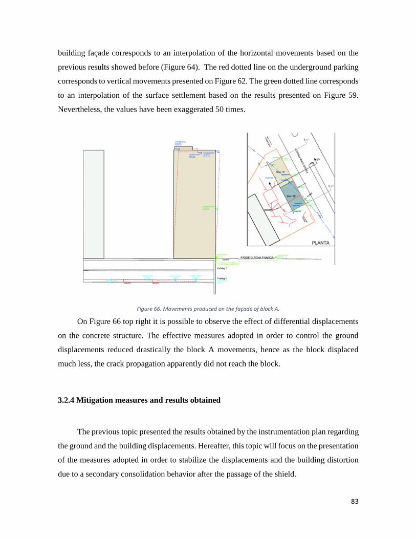
83
building façade corresponds to an interpolation of the horizontal movements based on the
previous results showed before (Figure 64). The red dotted line on the underground parking
corresponds to vertical movements presented on Figure 62. The green dotted line corresponds
to an interpolation of the surface settlement based on the results presented on Figure 59.
Nevertheless, the values have been exaggerated 50 times.
Figure 66. Movements produced on the façade of block A.
On Figure 66 top right it is possible to observe the effect of differential displacements
on the concrete structure. The effective measures adopted in order to control the ground
displacements reduced drastically the block A movements, hence as the block displaced
much less, the crack propagation apparently did not reach the block.
3.2.4 Mitigation measures and results obtained
The previous topic presented the results obtained by the instrumentation plan regarding
the ground and the building displacements. Hereafter, this topic will focus on the presentation
of the measures adopted in order to stabilize the displacements and the building distortion
due to a secondary consolidation behavior after the passage of the shield.

84
Figures 67 shows, that the face pressure is increased two times in order to control the
settlements. First, on day 09/03/2011 and increase from 2.7 to 2.9 bar. Then, one day after,
on 10/03/2011 another increase, now from 2.9 to 3.0 bar. This is the first measure in order
to try to control the building movements. The data shows that the measure successfully
control the induced movements due to tunneling on the point located from the building
midpoint to the last corner. However, a secondary consolidation behavior is observed,
making the ground to continue displacing after the passage of the shield.
Figure 68 presents the incidences occurred during the TBM advance below the
building. As said before, the thin layer of a very permeable clean sands located on top of the
tunnel face caused an over-excavation and furthermore problems with grout injection, as the
liquid grout seems to flow through the sand rather than create fill the annular gap. Resulting
in advance stops, in order to fix problems regarding the entrance of grout and soil through
the shield skin. Consequently the advance rate was highly impacted as showed on Figure 47.
Figure 67. Incidences occurred during the TBM advance.
Despite of the operational problems described above, it is not common such magnitude
of displacements in shield tunneling. In order to investigate the cause of such displacements,
after the passage of the shield below the building, it has been made some georadar tests.

85
The tests have been divided into two phases (Figure 68). The first phase is composed
of georadar test from the surface and from the underground parking lot. The second phase is
composed of georadar tests from inside the tunnel, after the mitigation measures have been
adopted.
The results obtained from the first phase of the test indicates that strong reflections,
that indicates areas of the subsoil with an important bulk behavior (yellow areas) with
possible void that are located at variable depth around 10 - 12 meters from the surface. The
rings identified are the numbers 976 to 978, 984 to 986, 991 to 993, 995 to 998 and 1000 to
1001.
In order to fill the soil voids created by the bulking behavior, mortar and cement grout
injections were performed from inside the tunnel. Figure 69 shows that most of the volume
injected per ring is around 0.5 - 1.5 m³.
Figure 68. Results obtained by georadar tests before and after the mitigation measures.
There is a big difference in volume injected on rings 991, 995 and 999. Those rings
were firstly injected with mortar on day 24/05/2011 with a volume of 9.7 m³, 4.8m³ and 4.5m³
respectively. In order to refill the annular gap around the ring, cement grout was injected on
day 28/05/2011 with 0.3 m³, 0.2 m² and 0.5 m³ respectively.

86
Figure 69. Injected volume per ring as a mitigation measure.
Returning once again to Figure 68, after the injections, a second phase of the georadar
tests have been performed from inside the tunnel. The results shows that the initial large areas
have been reduced to much smaller areas compared to the initial detected areas from the first
phase (red).
Nevertheless, the data shows that there are some unfilled areas, which can explain the
ground movements even after the injections.
3.3 FINAL COMMENTS
According to the data and results presented on the previous sections by the date of
13/04/2011. The following comments can be addressed:
During the shield advance, the data show an over-excavation is not produced in terms of
net weight extracted, however this does not take into account the clean sand layer that was
encountered when passing below the building.
Due to the high permeability of the thin layer, the liquid grout seems to flow through the
sand rather than create a correct annular gap backfill.
A better understand of the interaction between the TBM parameters and ground response
during the advances are noted, as the volume of bentonite around the shield is increases as

87
well as the face pressure P1. Resulting in very low displacements on block A compared to
block B.
The maximum settlement measured after the tunnel is completely excavated below the
building on 14/03/2011 exceeds the value of 25 mm on block B and 10 mm on block A,
showing some tendency to continue increasing.
On 14/03/2011 after the tunnel is excavated below the building, some measurement
points presents accumulated horizontal movements that exceed 35 mm with a tendency to
continue increasing.
On the underground parking structure, the distortion estimated is 1/680.
Considering the parking as a benchmark, results an inclination of the building of
approximately 1/445.
The georadar tests indicated an important presence of zones with voids after the passage
of the shield, which can help explain why the secondary consolidation behavior was causing
the building to continue displacing some months after the passage of the shield.
Those zones are located approximately 7 m from the surface to very close the installed
lining. However a big concentration of voids can be seen around 10 to 15 m above the tunnel
crown, between the rings 976 to 978, 984 to 986, 991 to 993, 995 to 998 and 1000 to 1001,
which are located between the p.k. 4840 and the p.k. 4920.

88
CHAPTER 4 – 3D NUMERICAL MODELLING BACK-ANALYSIS
This chapter describes the three dimensional model used during this research. The
results obtained from the Section 2 have been used for the validation of a 3D numerical
simulation procedure. The numerical back-analysis has been performed with the software
Plaxis 3D. It includes an explicit description of the different phases of the tunnel excavation
with the EPB TBM (face pressure, shield diameter reduction, backfilling grouting, and
installation of the lining).
This analysis is used to draw some conclusions regarding the behavior of the ground
and the building during the passage of the shield.
4.1 DESCRIPTION OF THE 3D MODEL
The Section 2 (Figure 40) has been modelled with the software Plaxis 2017. In order
to guarantee that the effects of tunneling will not be affected by boundary conditions, the
geometry is modelled with a large 140 x 100 x 60 meters rectangular box (Figure 71).
As presented in the previous chapter, the stratigraphic layer of the geological units near
the building is almost constant throughout the section. The only significant variation is due
to the variation in depth and thickness of the two deepest soils. In fact, the stratigraphic
contact between these two different soils gradually reduces its depth directly affecting the
excavation face.
It was noted that the software presents problems when trying to mesh complex layers.
In order to avoid such problems related to the difficulty of the software to create a discretized
volume with complex stratigraphy, it has been adopted a horizontal layers for all the units,
thus leads to simplifications that can lead to variability of the model results. Moreover, the
main simplification will be applied to the QR layer, due to its variability, as it can be seen in
Figure 40.

89
According to seasonal water cycles, in March of 2011, electronic piezometers and
open-tube piezometers recorded minimal variations in the water table level with a depth about
8 meters.
Figure 70. Geometry of the ground layers of the 3D model.
4.1.1 Geotechnical parameters of the soil layers
The physical properties and preliminary mechanical characteristics of the soil layers
have been investigated by means of site investigations and laboratory tests. According to the
L9 Project Plan, the data obtained will be presented next.
M2 Layer:
As presented previously the M2 group is composed of gravels, sand and shales. The
gravels are from angular clasts to sub angular, generally very heterogeneous and contain
some block. The lithology of the clasts is mainly slate, phyllite and hornfels and, to a lesser
extent, quartz, lithium and Paleozoic carbonated rocks.
The matrix is very sandy clay with color intensely red to reddish brown. The degree of
consolidation varies from below to breaches. It includes sections of metric thickness of coarse
sands with gravel and sparse gravel scattered and stretches of reddish holes are hardy
hardened with scarce sparse gravel. The layer is a 19.6 meter height, from level -40.4 to level

90
-60.0 m. The materials have a low permeability due to the low permeability of the clayey
matrix, around 3,9.10-7 and 1,7.10-9 m/s.
The SPT tests presented in Figure 71 shows N30 values ranging from 25 to
impenetrable, with an average value of 79. It is therefore a question of materials of medium
to high consistency as shown in Figure 72 Left.
Figure 71. SPT Results of M2 Layer.
Figure 72. Granulometric tests (Right) and Casagrande Plasticity chart (Left) - M2 Layer.
Based on the in-situ and laboratory tests, the L9 Project Plan estimated the geotechnical
parameters that can be seen in Table 3.
Table 3. Geotechnical Parameters - M2 Layer.
Property Range Average
Water moisture (%) 2,3 - 19,5 11,3
Dry density (g/cm³) 2,0 - 2,2 2,1
Particles density (g/cm³) 2,28 - 2,35 2,31

91
Granulometry
% < 20 mm 100 - 100 100
% < 5 mm 74 - 100 94,7
% < 2 mm 53 - 100 87,5
% < 0,4 mm 28,5 - 99,2 73,3
% < 0,08 mm 23,9 - 96,7 65,5
% < 0,002 mm 18,9 - 42,0 32,9
Atterberg limits
Plastic limit (%) 26- 37 31
Liquid limit (%) 14 - 21 18
Plasticity Index (%) 9 - 16 13
Uniaxial test UCS (kg/cm²) 0,4 - 19,5 12,6
Strain (%) 1,0 - 16,0 4,7
Direct shear test c (kg/cm²) 0,2 - 0,5 0,4
φ (o) 26,6 - 35,4 30
Oedometer test
e0 0,3 0,3
Cc 0,1 0,1
Cs 0,01 0,01
Po (kg/cm²) 1,2 1,2
M1s Layer:
The layer corresponds to medium to coarse sands and in less proportion, fine sand with
low content in the matrix. The material is usually yellow or orange and the degree of
cementation is generally low, although some levels are moderately cemented.
It includes some thin levels of cemented rounded gravel that rarely exceed 10
centimeters and lithology exclusively from the Paleozoic materials that emerge in the
Collserola Mountain. The layer is an 8.6 meter height, from level -31.8 to level -40.4 m.
These are somewhat permeable materials, having obtained permeability values around
10-6 and 2.10-5 m/s.
The SPT tests presented in Figure 73 shows N30 values ranging from 11 to
impenetrable, with an average value of 50.
Figure 73. SPT Results of M1 Layer.

92
Figure 74. Granulometric tests (Right) and Casagrande Plasticity chart (Left) - M1 Layer.
Based on the in-situ and laboratory tests, the L9 Project Plan estimated the following
geotechnical parameters:
Table 4. Geotechnical Parameters - M1s Layer.
Property Range Average
Water moisture (%) 11,2 - 25,6 17,9
Dry density (g/cm³) 1,6 - 2,0 1,6
Particles density (g/cm³) 2,65 - 2,69 2,67
Granulometry
% < 20 mm 90 - 100 98,7
% < 5 mm 77 - 100 95,5
% < 2 mm 62 - 100 92,6
% < 0,4 mm 18,6 - 99,9 69,7
% < 0,08 mm 2,6 - 99,7 39,2
% < 0,002 mm 1,9 - 32,4 20,0
Atterberg limits
Plastic limit (%) 20 - 40 29
Liquid limit (%) 12 - 22 17
Plasticity Index (%) NP - 21 12
Uniaxial test UCS (kg/cm²) 0,8 0,8
Strain (%) 6,5 6,5
Direct shear test c (kg/cm²) 0,3 - 1,2 0,7
φ (o) 34,5 - 36,4 35,5
Triaxial test c (kg/cm²) 0,0 - 0,1 0,1
φ (o) 30,8 - 34,2 32,5
QR Layer:
Sandy silts and sand with gravels constitute it, corresponding to sub active streams
deposits. In the central zone of the streams, the deposits are sub rounded gravels, mainly from

93
slates and to a lesser degree to Paleozoic carbonated rocks, while granite fragments are almost
non-existent.
The layer has a sandy brownish sandstone matrix and the cementation degree is very
low or zero. The layer is a 15.3 meter height, from level -16.5 to level -31.8 m.
Figure 75. Granulometric tests (Right) and Casagrande Plasticity chart (Left) - QR Layer.
These materials have a variable permeability depending on their fine content, being
low in the lateral zones and greater in the central areas of the streams. From the only Lefranc
test, a permeability value of 5.10-6 m/s has been estimated.
The SPT tests shows N30 values ranging from 24 to 44, with an average value of 32.
Therefore, lower values are expected due to the heterogeneity of this layer.
Based on the in-situ and laboratory tests, the L9 Project Plan estimated the following
geotechnical parameters:
Table 5. Geotechnical Parameters - QR Layer.
Property Range Average
Water moisture (%) 8,0 - 19,9 15,9
Dry density (g/cm³) 1,7 - 2,2 1,9
Particles density (g/cm³) 2,64 – 2,65 2,65
Granulometry
% < 20 mm 100 - 100 100
% < 5 mm 85 - 100 94,3
% < 2 mm 72 - 97 88,4
% < 0,4 mm 28,8 - 91,7 70,5
% < 0,08 mm 15,2 - 85,6 61,8
% < 0,002 mm - -

94
Atterberg limits
Plastic limit (%) 28 28
Liquid limit (%) 16 - 19 18
Plasticity Index (%) 9 - 12 10
Direct shear test c (kg/cm²) 0,4 - 1,0 0,7
φ (o) 11,1 - 37,4 24,3
Oedometer test
e0 0,5 0,5
Cc 0,1 0,1
Cs 0,02 0,02
Po (kg/cm²) 2,0 2,0
QL2 Layer:
The unit QL2 is formed by sand, mainly of fine grain to medium and to a lesser degree
of coarse grains, generally with a high proportion of clayey matrix. Occasionally, includes
small deposits of lenticular geometry of organic grayish clay soils. The layer is a 6.5 meter
height, from level -10.0 to level -16.5 m.
It is a very permeable level, having obtained an average permeability value of 9.8.10-5
m/s, although the pumping tests performed on this lithology in previous studies showed
values of this parameter of the order of 4.10-4 m/s.
The SPT tests presented in Figure 76 shows N30 values ranging from 3 to impenetrable,
with an average value of 25. What supposes a horizon of medium to low compactness. With
a certain increase in function of the depth.
Figure 76. SPT Results of Ql2 Layer.
Figure 77 shows the granulometric test and the Casagrande’s plasticity chart of these
materials.

95
Figure 77. Granulometric tests (Right) and Casagrande Plasticity chart (Left) - QL2 Layer.
Based on the in-situ and laboratory tests, the Construction Project estimated the
following geotechnical parameters:
Table 6. Geotechnical Parameters - QL2 Layer.
Property Range Average
Water moisture (%) 0,9 - 29,0 16,5
Dry density (g/cm³) 1,5 - 2,2 1,7
Particles density (g/cm³) 2,65 - 2,66 2,65
Granulometry
% < 20 mm 95 - 100 99,8
% < 5 mm 69 - 100 98,1
% < 2 mm 47 - 100 94,4
% < 0,4 mm 13,2 - 63,8 12,4
% < 0,08 mm 2,2 - 92,0 19,5
% < 0,002 mm 1,0 - 7,6 3,3
Atterberg limits
Plastic limit (%) 22 - 47 31
Liquid limit (%) 11 - 26 18
Plasticity Index (%) NP - 20 12
Uniaxial test UCS (kg/cm²) 0,2 - 0,9 0,4
Strain (%) 1,5 - 14,0 4,3
Direct shear test c (kg/cm²) 0,2 - 0,6 0,3
φ (o) 29,7 - 44,1 37,2
Oedometer test
e0 0,8 0,8
Cc 0,1 0,1
Cs 0,02 0,02
Po (kg/cm²) 2,0 2,0
QL1 Layer:
Brown silts with a very homogeneous appearance dominate it. Occasionally, they may
present a slightly sandy character. In the zones of greater potency, they pass to clayey silts

96
or clays of lighter or gray colorations that can contain abundant remains of organic matter.
The layer is a 10 meter height, from the surface to level -10.0 m.
Figure 78. Granulometric tests (Right) and Casagrande Plasticity chart (Left) - QL1 Layer.
It is a very permeable level, having obtained an average permeability value of 9.8.10-5
m/s, although the pumping tests performed on this lithology in previous studies showed
values of this parameter of the order of 4.10-4 m/s. The SPT tests shows N30 values around 5
and 18, with an average value of 10. What supposes a horizon of little compactness.
Based on the in-situ and laboratory tests, the Construction Project estimated the
following geotechnical parameters:
Table 7. Geotechnical Parameters - QL1 Layer.
Property Range Average
Water moisture (%) 5,4 - 38,8 19,8
Dry density (g/cm³) 1,3 - 2,0 1,7
Particles density (g/cm³) 2,63 - 2,71 2,67
Granulometry
% < 20 mm 94 - 100 99,5
% < 5 mm 82 - 100 98,3
% < 2 mm 74 - 100 96,8
% < 0,4 mm 16,7 - 100 83,1
% < 0,08 mm 12 - 99,9 68,5
% < 0,002 mm 17,7 - 53,5 33,1
Atterberg limits
Plastic limit (%) 22 - 58 35
Liquid limit (%) 16 - 31 21
Plasticity Index (%) 4 - 28 14
Uniaxial test UCS (kg/cm²) 0,1 - 2,9 1,3
Strain (%) 2,0 - 12,0 5,9

97
Direct shear test c (kg/cm²) 0 - 0,7 0,3
φ (o) 15,5 - 35,8 22,2
Triaxial test c (kg/cm²) 0,1 0,1
φ (o) 28,6 28,6
Oedometer test
e0 0,5 - 0,7 0,6
Cc 0,1 - 0,2 0,1
Cs 0,02 - 0,05 0,03
Po (kg/cm²) 0,8 - 1,4 1,1
4.1.2 Estimation of the constitutive models parameters
Based on the work of Limatola (2016), the initial HS-small parameters were estimated
based on the in-situ tests realized by the L9 Project Plan. The results obtained are presented
next:
Table 8. Initial HS-small parameters (Limatola, 2016).
Unit m E50Ref (MPa) Eoed
Ref (MPa) EurRef (MPa) 𝜸𝟎,𝟕 Go
Ref (MPa)
M2 0,90 277,7 100,0 833,2 6,77.10-4 323,5
M1s 0,80 45,9 25,3 180,0 3,40.10-4 85,0
QR 0,60 15,4 9,5 46,1 1,99.10-4 22,6
QL2 0,65 11,0 12,0 33,0 4,67.10-3 14,0
QL1 0,90 15,8 12,4 47,5 2,61.10-3 18,0
Nevertheless, due to the high degree of compressibility of the surface layer QL1, this
layer will be modelled using the Soft Soil model. Based on the average values of the
compressibility index (Cc) and swelling index (Cs), the modified parameters of the
constitutive model can be estimated by:
𝜆∗ =𝐶𝑐
2,3(1 + 𝑒) (86)
𝜅∗ =2𝐶𝑠
2,3(1 + 𝑒) (87)
Based on the equations (86) and (87) the Soft Soil model parameters for the QL1 layer
are presented on the Table 9.

98
Table 9. Soft Soil parameters for the layer QL1.
Unit Cc Cs e0 𝜆∗ 𝜅∗
QL1 0,1 0,03 0,6 0,02717 0,01630
4.1.2 Building design
Based on the building description, the twin reinforced concrete buildings will be first
modelled using a CAD software, in order to simplify the process. Furthermore, the building
model will be imported into the Plaxis 3D geometry. A combination of plate elements, beam
elements and anchor elements will be used once the model is imported to simulate the
structures.
Figure 79. Distance between the complex side and the boundary of the model (Where D is the tunnel diameter).
The distance between the complex corners and the boundary of the model can be seen
in Figure 79. The distances were estimated in function of the tunnel diameter (12 meters) in
a way that the displacements will not be affected by boundary effects.

99
Figure 80. Complex once imported into Plaxis 3D
Figure 80 shows the model once imported into Plaxis 3D. In order to avoid failure
due to large displacements, the entire complex will be considered in isotropic linear elastic
conditions.
The pillars (black vertical lines) has been modelled with beam elements spaced at
approximately 5 meters in both longitudinal and transversal direction. The horizontal beams
were also modelled using beam elements (dark pink lines). Beam elements have been chosen
because its ability to reproduce deflections due to shearing and also bending. In addition,
changes in length can be reproduced when axial stress are applied.
The portico structures (X profile) has been modelled with node-to-node anchor
elements (light pink and light yellow). The difference between the frontal porticos to the
lateral ones is the rigidity modulus EA. The node-to-node anchor elements have been chosen
due to its linear elastic behavior that can reproduce a spring connection. Hence, they are
defined by the constitutive relations between the axial stress and the longitudinal
deformations (elongation and shortening) of the element.
The building model considers self-weight equals to zero to all elements. In order to
simulate the stress transmitted to the ground, surface load (blue arrows) are applied in each
floor of the structure with a magnitude of 10 KN/m2 as can be seen in Figure 80.

100
The building’s floor (slabs) and the diaphragm walls have been modelled with plate
elements (yellow, green, orange and blue plates) as shown in Figure 81. By using this
element, 3 types of deformations are taken into account: shear deformation, compression due
to normal forces and bending.
The underground structures of this model include two sublevels of the parking lot and
four diaphragm walls. The dimensions in longitudinal and transversal directions takes into
account that the confinement of the buried volume is guaranteed by the presence of external
infill walls modeled with a maximum depth of 10 meters and equal to the depth of the floor
of the lower parking level. The lateral confinement will be modelled with a reinforced
concrete diaphragm wall. The height total of these structures therefore passes from the value
of 10 meters to that of 17 meters. Plate elements has been used to design the floor of the
parking and the diaphragm walls, while the parking pillars have been designed with node-to-
node anchor elements.
Figure 81. Underground structures of the complex.
The parameters used to design the different elements of the buildings are presented
next on Table 10, Table 11 and Table 12.
Table 10. Building plate elements parameters.
Element d (m) E (MPa) v
Building Slabs 0,5 300 0,0
Surface Slab 0,6 300 0,0
Underground Slab 0,6 300 0,0
Diaphragm Wall 0,6 136,4 0,1

101
Table 11. Building beam elements parameters.
Element E (MPa) v A (m²) I (m4)
Pillars 25 0,0 0,21 3.10-3
Longitudinal Beams 31 0,0 0,04 0,134.10-3
Table 12. Building anchor elements parameters.
Element EA (KN)
Underground Pillars 25.106
Front Porticos 3,13.106
Longitudinal Porticos 5,39.106
4.1.3 Tunnel and TBM design
The EPB TBM and the tunnel lining is modelled with the Tunnel Designer option of
the software. It is important to point here, that either the position of the tunnel and the
excavation process have been simplified due to the inability of the software to mesh thin
layers with respect the entire model dimensions. This issue happened particularly when it
was tried to simulate the TBM excavating the thin layer (less than 1 m) of clean sand at the
top of the tunnel cross section. Moreover, the thin layer corresponding to the hardened
volume of grout injected at the shield tail (approximately 25 cm) cannot be created.
The tunnel center is located at 3.5 times the external diameter, which corresponds to
42 meters below the surface. The circular cross section of the tunnel have been modelled
using two circles that represents the TBM diameter (12 m) and the segmental ring diameter
(40 cm) as shown in Figure 82.
The process of modelling the TBM consists of create the metallic TBM skin, which is
considered a rigid plate element. The shield skin thickness is 40 cm, the specific weight is
159 KN/m³, the Young’s modulus is 200 GPa and the Poisson’s ratio is zero.

102
Figure 82. Tunnel cross section in Tunnel Designer.
A soil-structure interaction is added outside of the tunnel due to cone shape of the TBM.
This means that the model considers a surface contraction from the shield front till the shield
skin.
The backfilling grout, as pointed before, will not consider the hardened grout volume
due to the inability of the software to mesh thin volumes, nevertheless, it will considers only
the liquid injection by means of a surface load, representing the grout pressure during the
excavation process (Figure 83 left). The face pressure is an earth pressure that increases
linearly with depth. The tunnel face pressure is modelled by means of a perpendicular load
as shown in Figure 83 right.
Figure 83. Design of the TBM considering surface contraction and backfilling grout injection (left) and face pressure (right).

103
The tunnel trajectory is composed of two different segments. The first one is an 18
meters straight path that is used to simulate the previous advance of the machine from Fonería
station. According to the L9 Project Plan and already presented in Chapter 3, the tunnel
passing below the building has curved path with 270 meters radius, inclined 38o respect the
horizontal axis. The TBM advance corresponds to the lining width, which is 1.8 m. Thus, the
curved path considers slices spaced 1.8 m from each other, as can be seen in Figure 84.
Figure 84. Tunnel trajectory.
The TBM advance methodology used to simulate the excavation and installation of the
final lining is presented next. It is also important to point once again that the tunneling process
have been simplified due to the computational constraints that the software imposes.
Step 1 – Face excavation:
Figure 85 present the first step of the tunnel excavation. It represents the face
excavation simultaneously with the face pressure been applied. In order to simulate the
soil/foam mix that waterproofs the face during the excavation, it is considered a dry face
condition (Figure 85 left).
During the first step, the plate element corresponding to the TBM skin is applied, as
well as the surface contraction with axial increment and the soil-structure interaction negative
interface.
On the other hand, changing to Plane Front view of the software, face pressure is
applied by means of a perpendicular surface load with vertical increment (Figure 85 right).

104
Figure 85. Face excavation modelling: Soil removal considering dry conditions (left) and face pressure application (right).
Step 2 – TBM conicity:
Step 2 correspond to the TBM conicity. In this step the face pressure is deactivated and
the other parameters are kept constant as in the previous step.
Step 3 to Step 5 – TBM cone shape profile:
From Step 3 to Step 5, the remaining cone shape of the shield is created. No other
parameter is altered during those steps.
Step 6 – TBM tail:
The last slice of the TBM has a constant diameter. Hence, it is considered that the outer
surface has a uniform surface contraction.
Step 7 – Backfilling grout and jack thrusting:
The backfilling injection as said before is created by means of a surface load,
corresponding to the liquid injection. In the Cross Section View, the outer surface is selected;
the negative interface is deactivated as well as the shield skin and the surface contraction.

105
Moreover, the surface load is activated considering a perpendicular load with vertical
increment.
Figure 86. Creation of the jack thrusting against the last installed lining in Plane Rear View (left) and 3D representation of the jacking thrusting been applied simultaneously with the grout injection (right)
The jacking thrusting against the last installed lining is designed in the Plane Rear
View, by means of a uniform constant load as shown in Figure 86 left. Moreover it is possible
to see in Figure 86 right the representation jacking against the lining in a three dimensional
view.
Step 8 – Installation of the lining:
This step correspond to the installation of the ring. In the Cross Section View, the
negative interface corresponding to the interaction grout-soil is activated, hence the surface
load corresponding to the backfilling grout is deactivated. The inner volume of the tunnel
that corresponds to the lining is activated and the material corresponding to the reinforced
concrete lining is selected (Figure 87).
Moreover, in Plane Rear view, the jack thrusting force is deactivated. Thus the tunnel
sequence is completed.

106
Figure 87. Installation of the tunnel lining.
Once the tunnel is designed, it can be generated into the 3D geometry previously
created. The result can be seen in Figure 88.
Figure 88. Perspective view of the 3D model with the tunnel generated (left) and Top View of the model (right)
The parameters used to model the TBM and the lining can be seen in Table 13. The
reinforced concrete lining is considered as volume layer. It is considered a non-porous lining
with linear elastic behavior.

107
Table 13. TBM characteristics.
d (m) 0,4
𝜸 (KN/m³) 159
E (GPa) 200
v 0,0
Contraction (%) 0,64
Contraction increment (%) -0,074
Jack load (KN) 850
Table 14. Lining characteristics.
d (m) 0,4
𝜸 (KN/m³) 25
FCK (MPa) 45
E (GPa) 41
v 0,15
4.1.4 Meshing
During this research, some issues appeared regarding the meshing process. The
complexity of the model due to different soil layers as well as the curved tunnel seems to
bring some computational complications that will be discussed further on.
Most of the problems appear when the hardened grout volume is trying to be
considered. A reasonable explanation is that due to the dimensions of the model, thin volumes
are impossible to mesh, especially in the curved zones where the volume has not a uniform
shape.
Due to the inability of the software to mesh a more complex model, as said before the
tunnel excavation process and the soil geometry were simplified, so that can be successfully
meshed. The mesh used is composed of medium triangle nodded elements as shown in Figure
90. The tunnel is refined with a coarseness factor of 0.4.

108
Figure 89. General overview of the mesh (left) and mesh generated for the building and the tunnel (right).
4.1.5 Simulating the excavation
The TBM advances and the soil-structure interaction will be modelled using the
Sequential Construction option. An initial phase is generated in order to calculate the initial
state of stress of the geometry. A K0 procedure is established, as the ground layers are all
horizontal. The pore pressures are calculated using the phreatic option, referring to the water
table level.
The next phases of the model will be designed considering drained conditions for all
layers.
Phase 1 considers the activation of the building into the geometry. As said previously,
the structures are considered zero weight, so that no further modification in the soil layers
weight should be applied. The displacements and small strains are reset to zero, in order to
consider that nor did the building nor the ground suffer any large displacement prior the
passage of the shield.

109
Phase 2 considers the first 18 meters already advanced by the shield inside the
continuum. As well as in the previous phase, the displacements and the small strains are reset
to zero.
Phase 3 to phase 71 will reproduce the TBM progress starting from day 07/03/2011
until 14/03/2011. The equivalence between the model phases and the days are shown in Table
15.
Table 15. Correspondence between the model phases with the real days.
Phase Corresponding
Day
7 08/03/2011
21 09/03/2011
35 10/03/2011
41 11/03/2011
50 12/03/2011
61 13/03/2011
71 14/03/2011
The Table 15 will be used as a baseline to present the results further. Each of the phases
corresponds to the position of the TBM face in the beginning of each correspondent day.
Figure 90. Representation of the TBM advance, applying grout pressure and face pressure.
As said before, the negative interface between the tunnel and the ground is created
considering two different parameters. The initial interface around the TBM skin considers
the material mode from the adjacent soil, while the interface around the installed lining

110
considers the material mode equals to a hardened grout. The interface corresponding to the
hardened grouting have been chosen due to the necessity to reproduce in some way the
hardened grout, because as it was explained earlier, modelling by means of a volume that
changes its stiffness with time was impossible.
Table 16. Characteristics of the hardened grout applied to the negative interface around the installed lining.
Material model Linear elastic
Drainage type Non-porous
𝜸 (KN/m³) 21
E (MPa) 500
v 0,20
Figure 91. Representation of the negative interface materials around the tunnel.
4.2 ANALYSIS OF THE CALCULATED RESULTS
During this research, several models were calculate in order to calibrate the numerical
results regarding the in situ measured. Three different approaches have been selected to be
presented in this research. Further on a discussion about the results obtained is presented.
The models consider the same ground parameters, but changes in TBM parameters,
such face pressure and grout pressure have been changed.
The first model considers the entire tunnel drive with constant face pressure and
constant grout pressure equals to 2.7 bar and 3.0 bar correspondently.

111
The second model considers a more realistic approach, with increasing the face
pressure according to the field data presented in Chapter 3. A simplification is made, instead
of increase the pressure from 2.7 to 2.9 bar, and then another increase to 3.0 bar, the model
considers a single increase directly from 2.7 to 3.0 bar on day 10/03/2011 that corresponds
to phase 35. The grout pressure is kept constant and equals to 3.0 bar.
The third model considers the same characteristics of the second model, differing that
on phase 35, the face pressure and the grout pressure are both increased to 5.0 bar in order to
investigate the influence of the TBM parameters in the model.
The last model presented on this dissertation, shows the results obtained when the face
pressure applied is 2 times the initial pressure (2.7 bar) and the grout pressure follows the
same increase.
A summary of the four models calculated on this dissertation is presented below on
Table 17.
Table 17. Summary of the four models presented on this dissertation.
Model Face Pressure (KN/m²) Grout Pressure (KN/m²) Observations
1 270 + 16 KN/m² m 300 + 20 KN/m² m Constant pressure during the whole drive
2 270 + 16 KN/m² m 300 + 20 KN/m² m Constant pressure until phase 34 (08/03/2011)
300 + 16 KN/m² m 300 + 20 KN/m² m Face pressure increase on phase 35 (10/03/2011)
3 270 + 16 KN/m² m 300 + 20 KN/m² m Constant pressure until phase 34 (08/03/2011)
500 + 16 KN/m² m 500 + 20 KN/m² m Face and grout pressure increase on phase 35 (10/03/2011)
4 270 + 16 KN/m² m 300 + 20 KN/m² m Constant pressure until phase 34 (08/03/2011)
540 + 16 KN/m² m 570 + 20 KN/m² m Face and grout pressure increase on phase 35 (10/03/2011)
4.2.1 Model 1 – Constant Pressure during the tunnel drive
As said before, this model considers the initial face pressure (270 KN/m²) and grout
pressure (300 KN/m²) constant during the whole tunnel drive.
Figure 92, shows the results related to the building right vertical displacements. The
dots corresponds to the in situ measured values presented in Figure 61, while the continuous
line represents the calculated values from the model.

112
Figure 92. Model 1 results for calculated vertical movements within the building right.
According to Figure 92 results, the model reproduces well the induced settlements
corresponding to the block B façade of the building as it can be seen in Figures 92a, 92b and
92c. However, it is possible to see a tendency of the model to overestimate the displacements
from the building midpoint to the last corner (Block A). The point T2F04923R050HT232Z
(Figure 92d) represents a point located approximately at the midpoint of the building, where
the tunnel curve radius is maximum. It is possible to observe that the curve influence the
model results, overestimating the displacements.
The absolute and relative errors have been calculated regarding the results from Figure
92, and then presented on Table 18.
The points located at the building front façade of block B (Figures 92a, 92b and 92c)
show a tendency of the model to increase the absolute error as the TBM moves away from
those points. Hence it is also possible to note that the point near the building left have been
affected by it. Thus the displacements calculated are slightly high compared to the in situ
measured from day 10/03/2011. On the other hand, the cumulative error of those points
ranges from 2 to more than 5.

113
Table 18. Errors calculated for the Model 1 vertical displacements.
T2F04897L021HT229Z
Date uz [mm] Model uz [mm] Measured eabs erelative
08/mar 0,05 -0,10 0,15 -1,49
09/mar -4,51 -3,70 0,81 -0,22
10/mar -15,61 -12,80 2,81 -0,22
11/mar -19,75 -19,80 0,05 0,00
12/mar -24,24 -21,70 2,54 -0,12
13/mar -26,49 -23,10 3,39 -0,15
14/mar -26,64 -23,50 3,14 -0,13
Σ 12,88 -2,32
T2F04897L082HT232Z
Date uz [mm] Model uz [mm] Measured eabs erelative
08/mar 0,05 -0,30 0,35 -1,15
09/mar -3,76 -2,90 0,86 -0,30
10/mar -13,33 -8,60 4,73 -0,55
11/mar -16,97 -13,50 3,47 -0,26
12/mar -20,78 -15,10 5,68 -0,38
13/mar -22,33 -15,90 6,43 -0,40
14/mar -22,35 -16,10 6,25 -0,39
Σ 27,77 -3,43
T2F04897L136HT233Z
Date uz [mm] Model uz [mm] Measured eabs erelative
08/mar 0,04 -0,10 0,14 -1,43
09/mar -2,94 -2,00 0,94 -0,47
10/mar -10,84 -5,60 5,24 -0,94
11/mar -13,93 -9,00 4,93 -0,55
12/mar -17,00 -10,10 6,90 -0,68
13/mar -17,79 -10,80 6,99 -0,65
14/mar -17,67 -11,00 6,67 -0,61
Σ 31,82 -5,32
T2F04923R050HT232Z
Date uz [mm] Model uz [mm] Measured eabs erelative
08/mar 0,25 -0,10 0,35 -3,48
09/mar -2,37 -0,20 2,17 -10,86
10/mar -10,20 -1,90 8,30 -4,37
11/mar -14,19 -4,00 10,19 -2,55
12/mar -20,72 -5,90 14,82 -2,51
13/mar -28,06 -7,00 21,06 -3,01
14/mar -29,79 -7,50 22,29 -2,97
Σ 79,17 -29,74

114
The point located at midpoint (Figure 92d) however, tends to increase radically the
errors from the beginning of the TBM advance. Nevertheless it is expected such results, as it
is presented on Chapter 3, advancing with a face pressure of 2.7 bar associated with other
factors already explained caused the building to settle more, so it is expected that a constant
face pressure drive will result in large displacements in the whole building.
The relative errors of this point presents a peak value on day 09/03, however the
important errors can be seen from day 08/03 to 14/03 as the calculated values are more than
4 times the in situ measured. Nevertheless it possible to see that the model is not reproducing
correctly building behavior, but showing that the settlements are uniform in the longitudinal
direction.
Figure 93 presents the results obtained for the building horizontal displacement. The
letter C at the end of each point indicate total movement given by the sum of the
displacements in the X and Y directions.
Figure 93. Model 1 results for calculated horizontal movements within the building right.

115
Table 19. Errors calculated for the Model 1 horizontal displacements.
T2F04897L021HT229C
Date uc [mm] Model uc [mm] Measured eabs erelative
8-mar 0,77 1,50 0,73 0,49
9-mar 8,20 4,90 3,30 0,67
10-mar 23,93 18,00 5,93 0,33
11-mar 28,97 30,50 1,53 0,05
12-mar 34,22 32,50 1,72 0,05
13-mar 38,15 32,50 5,65 0,17
14-mar 39,20 34,50 4,70 0,14
Σ 23,56 1,90
T2F04897L082HT232C
Date uc [mm] Model uc [mm] Measured eabs erelative
8-mar 0,77 1,50 0,73 0,49
9-mar 7,88 5,10 2,78 0,55
10-mar 22,58 20,00 2,58 0,13
11-mar 27,19 32,50 5,31 0,16
12-mar 31,89 35,00 3,11 0,09
13-mar 35,36 35,00 0,36 0,01
14-mar 36,33 36,50 0,17 0,00
Σ 15,03 1,43
T2F04897L136HT233C
Date uc [mm] Model uc [mm] Measured eabs erelative
8-mar 0,77 1,50 0,73 0,48
9-mar 7,61 5,00 2,61 0,52
10-mar 21,29 20,00 1,29 0,06
11-mar 25,46 32,50 7,04 0,22
12-mar 29,62 36,50 6,88 0,19
13-mar 32,65 36,50 3,85 0,11
14-mar 33,55 37,50 3,95 0,11
Σ 26,34 1,69
T2F04923R050HT232C
Date uc [mm] Model uc [mm] Measured eabs erelative
8-mar 0,80 1,00 0,20 0,20
9-mar 6,92 4,00 2,92 0,73
10-mar 20,39 7,50 12,89 1,72
11-mar 25,19 15,00 10,19 0,68
12-mar 31,38 16,00 15,38 0,96
13-mar 38,35 16,00 22,35 1,40
14-mar 40,21 16,00 24,21 1,51
Σ 88,13 7,20

116
According to Figure 93 results, the model reproduces well the induced settlements
corresponding to the block B façade of the building as it can be seen in Figures 93a, 93b and
93c. However, it is possible to see on Figure 93d the same tendency of the model to
overestimate the displacements from the building midpoint to the last corner (Block A).
Table 19 presents the errors calculated for the horizontal displacements. The absolute
error show that the model almost always calculate higher values compared to the in situ
measured. It is important to comment that the point located above the curve presents
unacceptable absolute errors, ranging from 10 to 24 mm.
On the other hand, the cumulative relative error of the points located in the building
façade corresponding to Block B (Figures 931, 93b, and 93c) presents very good results,
ranging from 1.4 to 1.9. However the point located above the curve (Figure 93d) the errors
tend to increase with time and the cumulative relative error is 7.2.
Figure 94. Model 1 results for calculated vertical movements in the parking slab of the building right.
Figure 94 shows the results calculated for the underground parking slab, which is
located at 10 meters below the surface. The points took for analysis corresponds to the ones

117
located at the corner of the right building as shown in the graphs circled in black. The points
are spaced at each 10 meters.
The vertical displacements calculated for the underground slab shows that the same
tendency regarding the movements as the points selected are closer to the curved path of the
tunnel. Figures 94a, 94b indicate that model reproduces well the movements where the tunnel
is straight or less curved. However, Figure 94c show a point which is located near the curve,
hence the results are overestimated.
A summary of the model 1 results regarding the soil-structure interaction is presented
next:
At a constant face pressure equals to 270 KN/m2 and a constant grout pressure equals to
300 KN/m2 the model presents acceptable results when the tunnel is straight or slightly
curved.
The cumulative absolute error for the building vertical movement presents a tendency to
increase as the tunnel becomes curved, with a cumulative maximum value for the point
T2F04923R050HT232Z with 79.17.
Relative errors regarding the building vertical movement ranges from 0.0 to 0.94 at point
located on the building front façade, however the relative errors increase abruptly when
points located near the maximum radius curve of the tunnel.
Relative error regarding the horizontal movement shows that the model always
overestimate the displacements near the maximum radius curve. A cumulative relative error
maximum is 7.20.
Regarding the underground slab, the same behavior noted in surface is followed in depth,
tending to overestimate the displacements as the curve of the tunnel approaches the point.
4.2.2 Model 2 – Increasing the face pressure on phase 35 (10/03/2011)
This next model tries to reproduce a more realistic approach in in terms of TBM
parameters according to the in situ data. The objective is to reproduce the displacement
reduction after the building midpoint. According to Figure 50 the initial face pressure (270

118
KN/m²) and grout pressure (300 KN/m²) while the tunnel starts passing below the building.,
after the initial displacements detected been too large, the face pressure is increased to 290
KN/m² and then increased again to 300 KN/m², while the grout pressure is kept constant.
In order to simplify the model, on phase 35, corresponding to day 10/03/2011 the face
pressure will be increased directly from 270 KN/m² to 300 KN/m².
Figure 95 shows the results related to the building vertical displacements. The dots
corresponds to the in situ measured values presented in Figure 61, while the continuous line
represents the calculated values from the model.
Figure 95. Model 2 results for calculated vertical movements within the building right.
The results of model 2 for vertical displacements shows that the increase of face
pressure cannot reproduce the settlement reduction in the point located above the curved path
of the tunnel (Figure 95d). Hence as the face pressure is increased on day 10/03/2011, the
TBM is already at least 36 meters ahead of façade of the Block B, thus the displacements
cannot be affected by it.
The error absolute and relative are calculate based on the figures presented above. The
results are presented on Table 20.

119
Table 20. Errors calculated for the Model 2 vertical displacements.
T2F04897L021HT229Z
Date uz [mm] Model uz [mm] Measured eabs erelative
08/mar 0,05 -0,10 0,15 -1,49
09/mar -4,51 -3,70 0,81 -0,22
10/mar -15,61 -12,80 2,81 -0,22
11/mar -19,75 -19,80 0,05 0,00
12/mar -24,24 -21,70 2,54 -0,12
13/mar -26,49 -23,10 3,39 -0,15
14/mar -26,64 -23,50 3,14 -0,13
Σ 12,88 -2,32
T2F04897L082HT232Z
Date uz [mm] Model uz [mm] Measured eabs erelative
08/mar 0,05 -0,30 0,35 -1,15
09/mar -3,76 -2,90 0,86 -0,30
10/mar -13,33 -8,60 4,73 -0,55
11/mar -16,97 -13,50 3,47 -0,26
12/mar -20,78 -15,10 5,68 -0,38
13/mar -22,33 -15,90 6,43 -0,40
14/mar -22,35 -16,10 6,25 -0,39
Σ 27,77 -3,43
T2F04897L136HT233Z
Date uz [mm] Model uz [mm] Measured eabs erelative
08/mar 0,04 -0,10 0,14 -1,43
09/mar -2,94 -2,00 0,94 -0,47
10/mar -10,84 -5,60 5,24 -0,94
11/mar -13,93 -9,00 4,93 -0,55
12/mar -17,00 -10,10 6,90 -0,68
13/mar -17,79 -10,80 6,99 -0,65
14/mar -17,67 -11,00 6,67 -0,61
Σ 31,82 -5,32
T2F04923R050HT232Z
Date uz [mm] Model uz [mm] Measured eabs erelative
08/mar 0,25 -0,10 0,35 -3,48
09/mar -2,37 -0,20 2,17 -10,86
10/mar -10,20 -1,90 8,30 -4,37
11/mar -14,19 -4,00 10,19 -2,55
12/mar -20,72 -5,90 14,82 -2,51
13/mar -28,06 -7,00 21,06 -3,01
14/mar -29,79 -7,50 22,29 -2,97
Σ 79,17 -29,74

120
The errors calculated for vertical displacements show that the values the same when
comparing with model 1, in which the face pressure is kept constant. It seems that the curved
path of the tunnel continues to affect the soil-structure interaction.
Figure 96 presents the results obtained for the building horizontal displacement. The
letter C at the end of each point indicate total movement given by the sum of the
displacements in the X and Y directions.
The results of model 2 indicates that the displacements are not changed due to the
increase of the face pressure. In addition, the results are almost the same of those presented
on model 1.
Figure 96. Model 2 results for calculated horizontal movements within the building right.
Table 21 presents the errors calculated for the horizontal displacements. The table
results indicates that the errors are approximately the same when compared to model 1.
Nevertheless, it is possible to assume that an increase in grout pressure proportional to
the increase in face pressure must be performed in order to adequate the results.

121
Table 21. Errors calculated for the Model 2 horizontal displacements.
T2F04897L021HT229C
Date uc [mm] Model uc [mm] Measured eabs erelative
8-mar 0,77 1,50 0,73 0,49
9-mar 8,20 4,90 3,30 0,67
10-mar 23,93 18,00 5,93 0,33
11-mar 28,97 30,50 1,53 0,05
12-mar 34,22 32,50 1,72 0,05
13-mar 38,15 32,50 5,65 0,17
14-mar 39,20 34,50 4,70 0,14
Σ 23,56 1,90
T2F04897L082HT232C
Date uc [mm] Model uc [mm] Measured eabs erelative
8-mar 0,77 1,50 0,73 0,49
9-mar 7,88 5,10 2,78 0,55
10-mar 22,58 20,00 2,58 0,13
11-mar 27,19 32,50 5,31 0,16
12-mar 31,89 35,00 3,11 0,09
13-mar 35,36 35,00 0,36 0,01
14-mar 36,33 36,50 0,17 0,00
Σ 15,03 1,43
T2F04897L136HT233C
Date uc [mm] Model uc [mm] Measured eabs erelative
8-mar 0,77 1,50 0,73 0,48
9-mar 7,61 5,00 2,61 0,52
10-mar 21,29 20,00 1,29 0,06
11-mar 25,46 32,50 7,04 0,22
12-mar 29,62 36,50 6,88 0,19
13-mar 32,65 36,50 3,85 0,11
14-mar 33,55 37,50 3,95 0,11
Σ 26,34 1,69
T2F04923R050HT232C
Date uc [mm] Model uc [mm] Measured eabs erelative
8-mar 0,80 1,00 0,20 0,20
9-mar 6,92 4,00 2,92 0,73
10-mar 20,39 7,50 12,89 1,72
11-mar 25,19 15,00 10,19 0,68
12-mar 31,38 16,00 15,38 0,96
13-mar 38,35 16,00 22,35 1,40
14-mar 40,21 16,00 24,21 1,51
Σ 88,13 7,20

122
Figure 97 shows the results calculated for the underground parking slab, which is
located at 10 meters below the surface. The points that is took for analysis corresponds to the
ones located at the corner of the right building as shown in the graphs. The point are spaced
at each 10 meters.
Figure 97. Model 2 results for calculated vertical movements in the parking slab of the building right.
A same behavior is observed in underground movements compared to model 1. The
slab behaves absolutely on a same way, in which the face pressure is kept constant.
A summary of the model 2 results regarding the soil-structure interaction is presented
next:
The increase of the face pressure from 270 KN/m² to 300 KN/m² on day 10/03/2011
(Phase 35) did not seem to change the results of the model. Moreover, the errors calculated
are the same when compared to those on model 1.
Horizontal movements like the vertical movements, are not changed due to the face
pressure increase.
Regarding the underground slab, the same behavior noted in surface is followed in depth,
tending to overestimate the displacements as the TBM advances through the curved path.

123
4.2.3 Model 3 – Increasing the face pressure and grout pressure on phase 35
(10/03/2011)
Based on the results of the previous models, it is possible raise questions about
uncertainties in ground conditions regarding the layer QR that increase the layer stiffness
below the building. However, it is very difficult to verify a drastically change in the ground
stiffness that can reduce the initial settlement of 26 mm in the initial corner of the building
to less than 10 mm in the building midpoint.
In addition to that, it is possible the absence of the hardened grout volume is affecting
the results in the curved path rather than in the straight path of the tunnel.
Figure 98 shows the results related to the building vertical displacements. The dots
corresponds to the in situ measured values presented in Figure 61, while the continuous line
represents the calculated values from the model.
Figure 98. Model 3 results for calculated vertical movements within the building right.

124
Table 22. Errors calculated for the Model 3 vertical displacements.
T2F04897L021HT229Z
Date uz [mm] Model uz [mm] Measured eabs erelative
08/mar 0,05 -0,10 0,15 -1,49
09/mar -4,51 -3,70 0,81 -0,22
10/mar -15,58 -12,80 2,78 -0,22
11/mar -19,11 -19,80 0,69 -0,03
12/mar -23,03 -21,70 1,33 -0,06
13/mar -24,98 -23,10 1,88 -0,08
14/mar -25,08 -23,50 1,58 -0,07
Σ 9,22 -2,17
T2F04897L082HT232Z
Date uz [mm] Model uz [mm] Measured eabs erelative
08/mar 0,05 -0,30 0,35 -1,15
09/mar -3,76 -2,90 0,86 -0,30
10/mar -13,30 -8,60 4,70 -0,55
11/mar -16,40 -13,50 2,90 -0,22
12/mar -19,73 -15,10 4,63 -0,31
13/mar -21,08 -15,90 5,18 -0,33
14/mar -21,08 -16,10 4,98 -0,31
Σ 23,60 -3,15
T2F04897L136HT233Z
Date uz [mm] Model uz [mm] Measured eabs erelative
08/mar 0,04 -0,10 0,14 -1,43
09/mar -2,94 -2,00 0,94 -0,47
10/mar -10,80 -5,60 5,20 -0,93
11/mar -13,45 -9,00 4,45 -0,49
12/mar -16,14 -10,10 6,04 -0,60
13/mar -16,82 -10,80 6,02 -0,56
14/mar -16,70 -11,00 5,70 -0,52
Σ 28,51 -5,00
T2F04923R050HT232Z
Date uz [mm] Model uz [mm] Measured eabs erelative
08/mar 0,25 -0,10 0,35 -3,48
09/mar -10,14 -0,20 9,94 -49,69
10/mar -10,20 -1,90 8,30 -4,37
11/mar -13,50 -4,00 9,50 -2,37
12/mar -19,11 -5,90 13,21 -2,24
13/mar -25,51 -7,00 18,51 -2,64
14/mar -26,97 -7,50 19,47 -2,60
Σ 79,27 -67,39

125
Based on the results of the model 3, it is possible to note that all the points selected for
curves have its settlement slightly reduced. Thus, the hypothesis about the absence of a
hardened grout volume affecting the results on the curved path can be confirmed according
to Figure 98d.
It is possible to note that the increase of the pressures to 500 KN/m² on day 10/03 tends
to stabilize the settlement as 10 mm, however as the TBM moves forward there is not volume
to inhibit the ground to move freely once the pressure is not applied any longer in the slice,
so with time the settlements starts to increase again, resulting in unrealistic results.
The errors on vertical movements of the model 3 results are presented on Table 22. The
errors calculated for the model 3 shows that, the increase of face and grout pressure to 500
KN/m² affect the model results. Thus, the ground could be stiffer in the area below the
building, especially because there is a presence of dispersed gravels.
Curiously, the point T2F04923R050HT232Z present a very large settlement on day
09/03 compared to model 2 (-2.37 mm and -10.14 mm respectively) which severely increase
the cumulative errors of the results for this point. Despite the cumulative errors have been
reduced, the errors for vertical movements still unacceptable on the curved path of the tunnel
(Figure 98d).
Figure 99. Model 3 results for calculated horizontal movements within the building right.

126
Table 23. Errors calculated for the Model 3 horizontal displacements.
T2F04897L021HT229C
Date uc [mm] Model uc [mm] Measured eabs erelative
8-mar 0,77 1,50 0,73 0,49
9-mar 8,20 4,90 3,30 0,67
10-mar 23,94 18,00 5,94 0,33
11-mar 28,21 30,50 2,29 0,08
12-mar 32,74 32,50 0,24 0,01
13-mar 35,86 32,50 3,36 0,10
14-mar 36,57 34,50 2,07 0,06
Σ 17,94 1,74
T2F04897L082HT232C
Date uc [mm] Model uc [mm] Measured eabs erelative
8-mar 0,77 1,50 0,73 0,49
9-mar 7,88 5,10 2,78 0,55
10-mar 22,60 20,00 2,60 0,13
11-mar 26,51 32,50 5,99 0,18
12-mar 30,56 35,00 4,44 0,13
13-mar 33,25 35,00 1,75 0,05
14-mar 33,89 36,50 2,61 0,07
Σ 20,91 1,59
T2F04897L136HT233C
Date uc [mm] Model uc [mm] Measured eabs erelative
8-mar 0,77 1,50 0,73 0,48
9-mar 7,61 5,00 2,61 0,52
10-mar 21,31 20,00 1,31 0,07
11-mar 24,85 32,50 7,65 0,24
12-mar 28,43 36,50 8,07 0,22
13-mar 30,72 36,50 5,78 0,16
14-mar 31,28 37,50 6,22 0,17
Σ 32,37 1,85
T2F04923R050HT232C
Date uc [mm] Model uc [mm] Measured eabs erelative
8-mar 0,80 1,00 0,20 0,20
9-mar 20,35 4,00 16,35 4,09
10-mar 20,39 7,50 12,89 1,72
11-mar 24,38 15,00 9,38 0,63
12-mar 29,62 16,00 13,62 0,85
13-mar 35,31 16,00 19,31 1,21
14-mar 36,70 16,00 20,70 1,29
Σ 92,46 9,98

127
Figure 99 presents the results obtained for the building horizontal displacement. The
letter C at the end of each point indicate total movement given by the sum of the
displacements in the X and Y directions.
According to the Figures 99a, 99b and 99c, a similar behavior occurs in terms of
horizontal displacements, however on day 13.03 and 14.03 it is possible to note a better
approximation of the numerical results regarding the in situ measured. However, Figure 99d
still presents unrealistic results and as it occurs in vertical movements, is possible to note that
the absence of the hardened volume of grout also affects the horizontal movements as the
TBM progresses.
Table 23 presents the errors (absolute and relative) calculated for the horizontal
displacements. Comparing the model 3 results with the model 2, the cumulative relative error
of the four points have been reduced from 1.90; 1.43; 1.69; 7.20 to 1.74; 1.59; 1.85; 9.98
respectively.
Figure 100. Model 3 results for calculated vertical movements in the parking slab.
Figure 100 shows the results for the underground parking slab, which is located at 10
meters below the surface. The points that is took for analysis corresponds to the ones located

128
at the corner of the right building as shown in the graphs. The point are spaced at each 10
meters.
The results of underground movements from the model 3 shows that the pressure
increase induce a slightly reduce the settlement of the three points of the parking slab.
Nevertheless, the results in the initial 20 meters of the slab is reproduced quite well (Figure
100a and 100b).
Figure 100c shows a same pattern for points located above the curved path of the
tunnel. An overestimation is produced even if the pressures is been increased.
A summary of the model 3 results regarding the soil-structure interaction is presented
next:
The increase of the face and grout pressures to 500 KN/m² seems to have a positive
effect on the model in terms of reducing the mvements of the building.
Even though the increase described above, the curved path of the tunnel still have a
significant impact on the model results.
Regarding the point T2F04923R050HT232Z located above the curved path, the
cumulative relative error for vertical movements is increased from -29.74 to -67.39.
Moreover, the cumulative relative error for horizontal movements is increased from 7.20 to
9.98.
Regarding the underground slab, the same behavior noted in surface is followed in depth,
tending to overestimate the displacements as the curve of the tunnel approaches the point
measured.
4.2.4 Comparison between the three models and the assessment of the causes of failure
in reproducing real movements
Model 1 and Model 2 shows that the increase of face pressure from 270 KN/M² to 300
KN/m² did not affect the ground response regarding the reduction of settlement on the second
half of the building length.

129
Model 3 on the other hand, considering an increase to 500 KN/m² in both face and
grout pressure produce an slightly reduction of the movements, however the point located
above the curve still presents unrealistic behavior compared to the in situ data.
A fourth model have been calculated considering but not presented on this research, in
which the face pressure is assumed two times the initial pressure (540 KN/m²) and the grout
pressure increases proportionally to 570 KN/m², both applied in phase 35. The fact that this
model is not presented is because once the pressures are increased, the TBM advances 7.2
meters (phase 35 to phase 38), and then, on phase 39 the ground collapses (Figure 101).
Figure 101. Ground failure due to an increase of the grout pressure to 570 KN/m².
Based on the results obtained, a comparison will be presented next, in order to assess
the changes of the TBM parameters affects the results of the model. As presented earlier, the
results of the building movements for points located near the straight or slightly curved path,
e.g. front façade, are reproduced quite well, independent of the change of the machines
parameters. However it is been noticed that somehow, in the curved path, the maximum
curved radius of the tunnel is affecting the results regardless the soil and the TBM parameters.
Figure 102 presents a comparison between the vertical movements calculated for the
point T2F04923R050HT232Z.

130
Figure 102. Comparison between the results calculated of the point T2F04923R050HT232Z.
It is possible that uncertainties regarding the ground conditions are presented below the
building, which are increasing the soil stiffness. The model 3, (green line) that considered
the possibility of such uncertainties by considering a face and grout pressure increase to 500
KN/m² on the curved path shows a slightly improvement of the results, but still far from the
in situ measured. Nevertheless the other two models that considers a more realistic approach
in terms of the TBM parameters produce the same results, regardless the face pressure been
constant during the whole drive (270 KN/m²) or by been increased to 300 KN/m² on phase
35.
Figure 103 presents a comparison between the horizontal movements calculated for the
point T2F04923R050HT232C.
Figure 103. Comparison between the results calculated of the point T2F04923R050HT232C.

131
A same pattern is been noticed for the building’s horizontal movements. The increase
of the pressures show a slightly positive effect on the model results but it is far away from
reproducing the in situ measured. Nevertheless, model 1 and model 2 presents almost
identical results.
Figure 104. Comparison between the results calculated of the point T2F04913R024HF001W.
Figure 104 presents a comparison between the vertical movements calculated for the
parking slab on point T2F04913R024HF001W.
The data from the models show that a same behavior is present on the underground
movements within the parking slab. Considering the increase of pressures leads to a slightly
reduction of the displacements.
A summary of the comparison regarding the soil-structure interaction is presented next:
By comparing the models, it is clear that simplifications regarding the TBM parameters
and operation are affecting the model, especially in the curved path of the tunnel.
The inability of the software to mesh small volumes, e.g. hardened grout, in a large
model such as this presented on this research seems to have no impact on straight path of the
tunnel. However, as the curvature radius increase, it is possible to assume that absence of a
stiff volume like the hardened grout is allowing the ground to displace as the pressure applied
on the slice is removed once the TBM advances.
It is important to point out here, that the model also simplifies the reality regarding the
presence of other adjacent structures, so the influence of other underground structures such

132
as pipelines and foundations of other nearby buildings could also helped to reduce the in situ
settlement profile.
4.2.5 Analysis of the surface and deep displacements outside the building
The results presented on the previous topics showed that the model 3 reproduces
slightly better the soil-structure interaction with the building above the tunnel. However,
unrealistic movements still been presented regardless changes in TBM parameters.
Based on model 3 results, surface and deep displacements outside the building are
going to be presented next, according to the in situ data measured presented on Figure 55,
Figure 59 and Figure 60.
Figure 105. Surface vertical movements calculated between PK 4850 and 4910.
Figure 105 shows the surface settlements above the tunnel axis from P.K 4850 to 4896.
The four graphs indicate a same tendency for vertical movements as occurs in the soil-
structure interaction presented earlier. Figures 105a, 105b and 105c correspond to point

133
located on a straight path or a slightly curved geometry of the tunnel alignment. It is possible
to note that the movements are very well reproduced by the model.
On the other hand, Figure 105d shows a measure point located very close to the
maximum curvature radius of the curve. Thus, some deviations occurs especially after day
10/03. Indicating that once the grout pressure is no longer applied on the slice, the ground
tends to continue settling.
Figure 106 shows the surface settlements above the tunnel axis from P.K 4915 to 4936.
Here it is possible to see the effect that the absence of a hardened grout volume and the curved
geometry of the tunnel also affects the magnitude of the calculated settlements on the surface.
The graphs show a similar phenomenon when comparing with the movements
calculated within the building. During phase 35 (10/03/2011), in which the face pressure and
grout pressure are increased, it is possible to see that the movements tends to stabilize.
However, as the shield tail moves away from the point, the absence of a volume of hardened
grout to control the ground movements in addition to the curved geometry causes an increase
of the settlement.
Figure 106. Surface vertical movements calculated between PK 4915 and 4936.

134
The graphs show a similar phenomenon when comparing with the movements
calculated within the building. During phase 35 (10/03/2011), in which the face pressure and
grout pressure are increased, it is possible to see that the movements tends to stabilize.
However, as the shield tail moves away and there in no pressure applied on the slice, the
point starts to settle again, leading to unrealistic results.
Figure 107 presents the longitudinal vertical settlement profile. The points used to plot
the graph are the same points presented above, so the same tendency of the model to
overestimate the settlement in the areas close to the curved path of the tunnel still present.
Figure 107. Comparison between the in situ measured and the calculated longitudinal settlement profile.
Figure 108 shows the horizontal movements measured at P.K. 4882, from the surface
to 25 meters below the surface. The results will be compared with those presented in Figure
60.

135
Figure 108. Horizontal movements calculated for the P.K. 4882
The Figure 108 indicate that the model tends to be accurate for the near surface
movements, between day 8 and 9. However, in depth, the movements tends to be
underestimated. Curiously, there is a deviation in the movement between -16 and -18 meters,
where is located the interface between the end of layer QL2 and the beginning of the layer
QR. Hence the movements suddenly increase its magnitude.
Between day 10/03 and 14/03, the model starts to overestimate the surface horizontal
movements reaching values around 40 and 45 mm. Thus a similar behavior curve is well
reproduced by the model, but as said before, at depth -16 and -18 m there is a suddenly change
of the behavior, that increases the magnitude of the displacements.
A summary of the results obtained for surface settlements and horizontal movements
in depth is presented next:
The surface settlement calculated tends to follow a similar behavior when it is compared
with the building movements.
The model also tends to be accurate to slightly curved path, as shown in Figure 131. As
the TBM passes below the building midpoint that coincides with the maximum curvature
radio, the movements tends to be overestimated.

136
Horizontal movements in depth as shown in Figure 132, indicate that the model
reproduce the behavior curve, thus tends to overestimate the results. However an anomaly is
produced on the interface between the layer QL2 and QR, in which the movements increase.

137
CHAPTER 5 – CONCLUSIONS
This research deals with the study of the soil-structure interaction between the 12 m
diameter TBM that excavated part of the Barcelona Metro L9 and the building located at
Passeig Zona Franca. The boring machine passed below this building on the 08/03/2011 and
passed by it on the 14/03/2011.
The first part of the research focused on the collection and analysis of the observed
measurements during the passage of the shield below the building. Also, the TBM parameters
observed during the tunnel drive were analysed.
During tunnelling, the boring machine crossed a thin layer of gravels with a clean sand
matrix, located at the higher part of tunnel face. This thin layer, which was not detected
during the project, complicated the advancement of the boring machine. Actually, the control
of the EPB-TBM operating pressures was extremely difficult due to the high permeability of
the thin layer of gravels. Consequently, the first meters of excavation below the building
caused unusual high settlements that reached values of approximately 24 mm at the ground
level and 26 mm at the parking level. These movements caused some damage in the building
in the form of visible cracks.
Due to the unexpectedly high initial ground movements, the TBM face pressure and
the volume of bentonite injected were increased. At first, the face pressure was increased
from 2.7 to 2.9 bars and then, during the last part of the excavation below the building, the
face pressure was increased up to 3.0 bar. On the other hand, the volume of injected bentonite
was increased from 1000 to 1800 liters, including sporadic values of up to 2800 liters. The
observed movements show that the measure adopted was successful, reducing the observed
settlement from 24 to approximately 7 mm.
After the passage of the shield, the building continued to settle, especially in the area
between its first corner (closer to the tunnel) and its midpoint. Vertical movements of up to
38 mm were measured in points of the building located at the ground level above the tunnel
axis and settlements of 33 mm were observed within the parking slab at a depth of 10 m.
In order to investigate the cause of these high settlement values, georadar tests were
run in the area close to the excavation. Cavities of different dimensions were detected in the

138
ground above the constructed tunnel. To limit any possible extra soil movements, cement and
grout were injected into the ground from within the tunnel, from the soil surface and also
from the underground parking to fill up the cavities.
The second part of this research focuses on the creation of a three dimension numerical
model in Plaxis 3D to back-calculate the in situ measured displacements.
Problems regarding meshing complex geometries were identified during the creation
of the finite element model. Thus, in order to carry on with the numerical analyses, some
simplifications had to be made:
The hardened volume of grout behind the shield tail and the thin layer of clean sand at
the top of the tunnel face could not be considered in the model for numerical reasons.
Grout injections were considered only by means of a liquid pressure.
The results from the 3D numerical analyses allow drawing the following conclusions:
The three models presented very few differences regarding the ground response due to
face pressure and grout pressure changes. All the models overestimate ground movements in
curved alignment of the Line 9 tunnel.
Increasing the face pressure and grout pressure to 500 KN/m² causes a reduction of
ground movements in the curved alignment of the tunnel, but only in the area close to where
the grout pressure is applied. Far from the shield tail, the computed settlements are bigger
than the observed ones.
The effect of a hardened volume of grout around the tunnel lining on the ground
movements has not been studied due to unsolved numerical problems.
In general, computed ground movements do reproduce well the observed measurements
in the straight alignment of the tunnel.
During this research, simplifications had to be made in order to successfully run the
complex numerical model.
Such simplifications might have affected the final results, producing an overestimation
of the ground movements in the curved alignment of the tunnel. The TBM operating
pressures do affect the computed ground movements. Nevertheless, high values of these
pressures do not reduce the overestimation of soil displacements.

139
5.1 Further studies and improvement of the numerical results
Considerable scope remains for further research of numerical models with complex
geometry, especially curved tunnels. Some suggestions to extend the research presented in
this dissertation are given below.
The increase of face pressure and grout pressure tested in this research were useful for
identifying the model response in terms of reduction of the displacements. Similar tests could
be performed considering the bentonite injection in the model, by means of a surface load
applied around the TBM skin.
The curved geometry of the tunnel is a problem in terms of mathematical solutions in
the Plaxis 3D that increase the displacements of the model. However, the influence in other
types of problems have not been clearly identified. Some research and development of
problems with curved tunnels would help to improve calibrations in back-analysis between
field data and numerical results.
The results seems to indicate that a volume of grout which increases its stiffness with
time could help to control the ground displacements of the model. However as described
earlier, the version of Plaxis used cannot mesh the model when a thin volume corresponding
to the grout is considered. The simulation of the same geometry in different FEM softwares
with a powerful mesher could be performed in order to analyze if the thin volume is
generated.

140
BIBLIOGRAPHY
Anagnostou, G & Kovári, K. (1996). Face stability in slurry and EPB shield tunnelling.
Tunnels & Tunnelling International. Volume: 28 (12).
Benz, T. (2006). Small-strains stiffness of soils and its numerical consequences. Ph.D
Thesis, University of Stuttgart.
Bezuijen, A. & Talmon, A. M. (2005). Grout Pressures around a Tunnel Lining,
Influence of Grout Consolidation and Loading on Lining. Tunnelling. A Decade of Progress.
GeoDelft 1995-2005. London: Taylor & Francis, 109-114.
Bezuijen, A. (2011), Foam used during EPB tunneling in saturated sand, description of
mechanisms. Proceedings. WTC 2011, Helsinki.
Bono, R., Ortu, M., Valdemarín, F. (2008). Surface settlement minimization in soft soil
when excavating with an earth pressure balance shield. Jornada Técnica de Túneles con EPB.
Simulación y Control de la Tuneladora. 105-128.
Castellanza, R., Bett, D., Lambrugli, A. (2008). Three-dimensional numerical models
for mechanised excavations in urban areas. Jornada Técnica de Túneles con EPB. Simulación
y Control de la Tuneladora. 105-128.
Chapman, D., Metje, N., Stark, A. (2010). Introduction to Tunnel Construction. Spon
Press, Abingdon. 417 p.
Di Mariano & Gens, A. (2014). EPB tunnelling in mixed geological formations: A case
study. Geotechnical Aspects of Underground Construction in Soft Ground. Seoul, Korea.
Duarte, M. A. P. (2007). Foam as a soil conditioner in tunnelling: physical and
mechanical properties of conditioned sands. Ph.D thesis, University of Oxford.
Duncan, J. M. and Chang, C. Y. (1970). Nonlinear analysis of stress and strain in soil.
Journal of the Soil Mechanics and Foundation Division, 96, p. 1629-1653.
Farrell, R. P. (2010). Tunnelling in sands and the response of buildings. Ph.D Thesis,
University of Cambridge.

141
Farrell, R. P., Mair, R. J., Sciotti, A., Pigorini, A. & Ricci, M. (2011). The response of
buildings to tunnelling: a case study. Proceedings of 7th International Symposium on
Geotechnical Aspects of Underground Construction in Soft Ground.
Festa, D., Broere, W., Bosch, J. W. (2014). A numerical model for the tunnel boring
machine interaction with soil. Geotechnical Aspects of Underground Construction in Soft
Ground. Seoul, Korea.
Franzius, J. N., Potts, D. M., Burland, J. B (2005). The response of surface structures
to tunnel construction. Proceedings of the Institution of Civil Engineers: Geotechnical
Engineering (158): London, 15 p.
Gens, A., Di Mariano, A. Persio, R. Castellanza, R and Arroyo, M. (2009). Relación
entre parámetros de una tuneladora EPB y los movimientos del terreno. 3as Jornadas
Hispano-Portuguesa de Geotecnia. Madrid: 433-441.
Gens, A. Bot, R., Schwarz, H. (2005). Construction of a new Metro line in Barcelona:
design criteria, excavation and monitoring system. Geotechnical Aspects of Underground
Construction in Soft Ground. Proceedings of the 5th International Conference of TC28 of the
ISSMGE Amsterdam.
Goh, K. H. (2010). Response of ground and buildings to deep excavations and
tunneling. Ph.D thesis, University of Cambridge.
Goh, K. H. & Mair, R. J. (2011). The horizontal response of framed buildings on
individual footings to excavation-induced movements. Proceedings of 7th International
Symposium on Geotechnical Aspects of Underground Construction in Soft Ground.
Guglielmetti, V., Grasso, P., Mahtab, A. Xu, S. (2007). Mechanized Tunnelling in
Urban Areas: Design Methodology and Construction Control. London: Taylor & Francis,
507 p.
Ishihara, K. et al. (1975). Undrained deformations and liquefaction of sand under cyclic
stresses. Soils and Foundations, 15(1): p. 29-44.
Janbu, N. (1963). Soil compressibility as determined by oedometer and triaxial tests.
Proceedings 3rd ECSMFE, volume 1, p. 19-25.

142
Kondner, R. I. and Zelasko, J. S. (1963). A hyperbolic stress-strain formulation for
sands. 2nd Pan American Conference in Soil Mechanics and Foundation Engineering. Brazil,
volume 1, p. 289-394.
Limatola, V. (2016). Building response to tunneling: the case of Line 9 EPB tunnelling
in Barcelona. Master’s thesis, University Napoli Federico II.
Mair, R. J., Taylor, R. N., Burland, J. B (1996). Prediction of ground movements and
assessment of risk of building damage due to bored tunneling. Proceedings of the
International Symposium on Geotechnical Aspects of Underground Construction in Soft
Ground: London, 6 p.
Mair, R. J. & Taylor R. N. (1997). Bored tunnelling in the urban environment. State-
of-the-art Report and Theme Lecture. Proceedings of 14th International Conference on Soil
Mechanics and Foundation Engineering, Hamburg, Balkema, Vol. 4. 2353-2385.
Mair, R.J. (2008). Tunnelling and geotechnics: new horizons. Géotechnique 58, No. 9,
695-736.
Merritt, A. S. & Mair, R. J. (2006). Mechanics of tunnelling machine screw conveyors:
a theoretical model. Géotechnique 58, No. 2, 79–94.
Merritt, A. S. & Mair, R. J. (2006). Mechanics of tunneling machine screw conveyors:
model tests. Géotechnique 56, No. 9, 605–615.
Merritt, A. S. (2004). Conditioning of clay soils for tunnelling machine screw
conveyors. Ph.D Thesis, University of Cambridge.
Peck, R. B. (1969). Deep excavations and tunnelling in soft ground. 7th International
Conference on Soil Mechanics and Foundation Engineering, Mexico City. 225–290.
Potts, D. M. & Addenbrooke, T. I. (1997). Structure’s influence on tunneling induced
ground movements. Proceedings of the Institution of Civil Engineers, Geotechnical
Engineering, pages 109-125, 125, (2). Thomas Telford, London.
Seed, H. B. and Idriss, M. N (1970). Soil moduli and dumping factors for dynamic
response analysis. Report 70-1, EERC, Berkeley.

143
Soreide, O. K. (1990). Mixed hardening models for frictional soil. . Ph.D Thesis,
Norwegian University of Science and Technology.
Schanz, T., Vermeer, P. A, Bonnier, P. G. (1999). The hardening soil model:
Formulation and verification. Beyond 2000 in Computational Geotechnics – 10 Years of
Plaxis. Balkema, Rotterdam.16 p.
Shirlaw et al. (2004). Recent cxperience in automatic tail void grouting with soft
ground Tunnel Boring Machines. Proceedings World Tunnel Congress 2004, volume 2.
Tatsuoka, F. and Ishihara, K. (1974). Yielding of sand in triaxial compression. Soils
and Foundations, 14 (2): p. 63-73.
Thewes, M. (2008). Shield Tunnelling Technology for the Mitigation of Geotechnical
Risks. Proceedings of Tuneles en zonas urbanas densamente pobladas – experiencias
internacionales, Technical School of Civil Engineering, Barcelona.
Thewes, M. & W. Burger (2005). Clogging of TBM drives in clay - identification and
mitigation of risks. Underground Space Use, Proceedings of the 2005 ITA World Tunnel
Congress, Istanbul, Turkey, Balkema, pp. 737-742.
Vermeer, P. A. (1980). Formulation and analysis of sand deformation problems. Ph.D
Thesis, Delft University of Science and Technology.