3D modelling of leaves from color and ToF data

for robotized plant measuring

G. Alenya, B. Dellen and C. Torras

Abstract—Supervision of long-lasting extensive botanic ex-periments is a promising robotic application that some recenttechnological advances have made feasible. Plant modellingfor this application has strong demands, particularly in whatconcerns 3D information gathering and speed. This paper showsthat Time-of-Flight (ToF) cameras achieve a good compromisebetween both demands, providing a suitable complement tocolor vision. A new method is proposed to segment plant imagesinto their composite surface patches by combining hierarchicalcolor segmentation with quadratic surface fitting using ToFdepth data. Experimentation shows that the interpolated depthmaps derived from the obtained surfaces fit well the originalscenes. Moreover, candidate leaves to be approached by ameasuring instrument are ranked, and then robot-mountedcameras move closer to them to validate their suitability tobeing sampled. Some ambiguities arising from leaves overlapor occlusions are cleared up in this way. The work is aproof-of-concept that dense color data combined with sparsedepth as provided by a ToF camera yields a good enough3D approximation for automated plant measuring at the highthroughput imposed by the application.

I. INTRODUCTION

Recent advances in depth sensors [1], deformable object

modelling [2], and autonomous mobile manipulation [3] have

considerably widened the scope of robot application. One

area that is nowadays gaining attention since it could benefit

from all these advances is the monitoring and maintenance of

large botanic experimentation fields, e.g., for plant phenotyp-

ing. The goal is to determine the best treatments (watering,

nutrients, sunlight) to optimize predefined aspects (plant

growth, seedling, flowers) and, towards this aim, experiments

entailing many repetitive actions need to be conducted [4].

Measurements and samples from leaves must be regularly

taken and some pruning needs to be performed. These are

tasks for which robots would be very handy, difficulties

arising from the complex structure and deformable nature

of plants, which do not only change appearance through

growing, but whose leaves move also on a daily cycle.

As regards to sensing, color vision has been used to obtain

some relevant plant features, but when it comes to extracting

structural/geometric information for modelling and manip-

ulation purposes, the concourse of a user is required to

provide hints on segmentation from multiple views [5]. If a

This research is partially funded by the EU GARNICS project FP7-247947, by the Spanish Ministry of Science and Innovation under projectsDPI2008-06022 and MIPRCV Consolider Ingenio CSD2007-00018, and theCatalan Research Commission. G. Alenya was supported by the CSIC undera Jae-Doc Fellowship. B. Dellen acknowledges support from the SpanishMinistry for Science and Innovation via a Ramon y Cajal fellowship.

Authors are with Institut de Robotica i Informatica Industrial,CSIC-UPC, Llorens i Artigas 4-6, 08028 Barcelona, Spain;{galenya,bdellen,torras}@iri.upc.edu

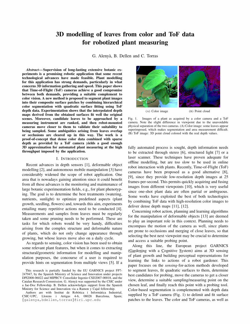
(A) Color image (B) Point cloud

Fig. 1. Images of a plant as acquired by a color camera and a ToFcamera. Note the slight difference in viewpoint due to the unavoidablephysical separation of the two cameras. (A) Color image: some leaves appearsuperimposed, which makes segmentation and area measurement difficult.(B) ToF image: 3D point cloud colored with the real depth values.

fully automated process is sought, depth information needs

to be extracted through stereo [6], structured light [7] or a

laser scanner. These techniques have proven adequate for

offline modelling, but are too slow to be used in online

robot interaction with plants. Recently, Time-of-Flight (ToF)

cameras have been proposed as a good alternative [8],

[9], since they provide low-resolution depth images at 25

frames-per-second. This permits quickly acquiring and fusing

images from different viewpoints [10], which is very useful

since one-shot plant data are often partial or ambiguous.

Some works have exploited the best of both technologies

by combining ToF data with high-resolution color images to

deliver dense depth maps [11], [12].

Concerning robot action, planning and learning algorithms

for the manipulation of deformable objects [13] are deemed

to play an important role in this context. Planning needs to

encompass the motion of the camera as well, since plants

are prone to occlusions and merging of close leaves, so that

selecting the best next viewpoint may be crucial to determine

and access a suitable probing point.

Along this line, the European project GARNICS

(Gardening with a Cognitive System) aims at 3D sensing

of plant growth and building perceptual representations for

learning the links to actions of a robot gardener. This

paper focuses on the sensing-for-action methods developed

to segment leaves, fit quadratic surfaces to them, determine

best candidates for probing, move the cameras to get a closer

view, determine a suitable sampling/measuring point on the

chosen leaf, and finally reach this point with a probing tool.

Color-based segmentation is complemented with depth data

supplied by a ToF camera (Fig. 1) to delimit and fit surface

patches to the leaves. The color and ToF cameras, as well as

Fig. 2. WAM arm used in the experiments holding the color and ToFcameras, as well as a fake measurement instrument in the form of a stick.

the probing tool, are all mounted on the robot end-effector, so

that an egocentric coordinate frame is used for all motions.

The paper is structured as follows. In Section II, an

overview of the system is provided. Next, in Section III,

we explain how images obtained with the depth and the

color camera are fused. In Section IV, the depth-aided color

segmentation algorithm is described, followed by Section V,

where the plant monitoring procedure is explained. Experi-

mental results are presented in Section VI and discussed in

Section VII.

II. SYSTEM OVERVIEW

The experimental setup includes a PMD CamCube Time-

of-Flight camera and a PointGrey Flea camera rigidly at-

tached to the last link of a Barrett WAM arm (Fig. 2). As

can be observed, the cameras are displaced from the robot

end-effector position to leave room for the future placement

of measuring devices, which are here replaced by a 30 cm

long stick.

The aim of the present work is to develop a completely

automated procedure to segment and model some leaves

of a plant using a general view and possibly other close-

up views obtained by moving the camera system with the

robot arm. For the general view, we assume that the plant

is located in a known position, so that the first image

is always taken from the same point of view. This is a

reasonable assumption since, in large phenotyping facilities,

plants are usually located in multiple-position trays or they

move in a conveyor belt. Close-up views are taken to verify

the accessibility of the best leaf candidates, by removing

ambiguities due to merged leaves or occlusions.

The process consists of three stages. First, color and depth

images are acquired and combined to obtain a colored point

cloud. The method to determine the required calibration

matrices Krgb and F is explained in Section III.

Second, the different leaves are segmented from the point

cloud, and a plane or a quadratic surface is fitted to each

of them. The surface model provides the position and ori-

entation of each leaf. This first segmentation may contain

some errors, e.g., several superimposed leaves may fall in

the same region, and regions including few points may lead

to a relatively large fitting error.

Third, using the position and orientation of the best leaf

candidate, the robot moves the camera system closer to it to

obtain a more detailed view, which is used to obtain a better

model and eventually separate different leaves. The method

to determine the required transformation matrices Hl1 and

Hl2 is explained in Section V-B.

In the future we will consider also the images perceived

along the robot motion from the initial view to the detailed

view. In this framework, the use of a time-of-flight camera

will be advantageous.

III. IMAGE FUSION

The cameras need to be calibrated in order to fuse depth

and color information. Taking advantage of the fact that

the ToF camera provides registered depth and grey-level

images, we apply a standard stereo calibration algorithm

making use of a small calibration pattern at close distances.

The calibration error is lower for the RGB camera than

for the ToF camera due to the reduced resolution of the

latter, so to perform the internal parameter calibration more

sample images are captured with the ToF camera to try to

compensate for this to some extent. With this procedure, the

required matrix Krgb of intrinsic parameters is determined,

and also the extrinsic matrix F that in our case provides the

position of the ToF camera with respect to the color camera.

The fusion of the depth with the color data is performed

by transforming the 3D point coordinates to the RGB camera

reference frame, and then projecting these points to the

camera image plane. Within this framework, color points not

having a 3D counterpart are discarded. If necessary, denser

point clouds can be obtained through linear interpolation

between consecutive 3D points or using a more elaborate

method based on 3D meshes [14].

However, as both cameras have slightly different view-

points (Fig. 1), some points are seen by one camera but not

by the other, and consequently it is impossible to find their

correspondence. These occlusions appear mainly for closer

objects, precisely our scenario.

In our method they are detected and removed using a

Z buffer approach. First, the point cloud is transformed

to the RGB camera reference frame using the extrinsic

transformation matrix F. Ideally, this leads to 3D points

projecting on the corresponding pixel in the color image.

In the case of occlusion, only the point that is closer to

the camera is stored in the Z buffer. However, as the ToF

camera has a lower resolution (204 × 204) than the color

camera (640 × 480), two different 3D points (namely, the

foreground and the occluded background points) may not

project exactly onto the same color point, so no one is

removed. This leads to a mosaic of foreground-background

pixels in the regions where occlusions occur. We have taken

into account a neighborhood region to build the Z buffer, so

that the depth of neighbours determine whether occlusions

are to be considered (Fig. 3).

For very close views, we further removed all 3D points

close to the background (using background subtraction) to

enforce the suppression of any wrong colored point.

IV. DEPTH-AIDED COLOR SEGMENTATION

We describe an algorithm for the segmentation of color

images into surface patches using sparse depth data. Images

Fig. 3. Result of assigning to each 3D point its corresponding color.Occlusions, i.e., depth points that are not viewed by the color camera, aremarked as red points.

are segmented in the color space, but the segmentation

procedure is aided by the depth data. Since the segmentation

is performed in the dense color space, even sparse or noisy

depth information can be used. This kind of data often

poses problems to segmentation algorithms operating in the

depth data space directly. The core idea of our method is

based on the notion that surface boundaries are in most

cases represented by an edge in the color image. Since we

are dealing with sparse depth data, it is further desirable

to have as large segments as possible - otherwise model

fitting becomes impracticable due to lack of data inside

segments. We thus segment the color image with different

resolutions (see Section IV-A). Quadratic surface models are

fitted to each segment (Section IV-B), and we select those

segments from the hierarchy which minimize the total fitting

error, while taking into account the hierarchy level, i.e.,

segments obtained at lower resolutions are given preference

to segments at higher ones (Section IV-C). The resulting new

segmentation is then further improved by applying an addi-

tional region merging step through which segments having

highly different color values can be merged if they describe

the same surface (see Section IV-D). Then, unclustered points

are assigned to the closest surface, using both depth and color

information (see Section IV-E).

A. Hierarchical color segmentation

The color image is segmented using the method of su-

perparamagnetic clustering of data employed in [15] which

allows a segmentation hierarchy to be generated by segment-

ing the image with different resolutions. For this purpose,

we varied the interaction strength by multiplying the mean

distance △ by a factor between 1.4 and 0.6.

B. Model fitting and selection

For each color segment si and model type (see Section IV-

F) we perform a minimization of the mean square distance

Ei,model = 1/N∑

j

(zj − zj,m)2 (1)

of measured depth points zj,m from the estimated model

depth zj = fi,model(xj , yj), where fi,model is the data-model

function and N is the number of measured depth points in

the area of segment si. The optimization is performed with

a Nelder-Mead simplex search algorithm.

The mean square errors for two different model types,

i.e. Ei,plane and Ei,curved, are computed. We select the planar

model if Ei,plane < Ei,curved+τ1, the curved model otherwise.

The larger parameter τ1, the more preference is given to

planar surfaces than to curved surfaces.

C. Color-segment selection procedure

We define the following selection procedure considering

first only two levels u and u+1, where a higher level denotesa higher resolution. Let sui be a segment at level u of the

hierarchy having a fitting error Eui (see Section IV-B). At

the level u+ 1 of the hierarchy, segment sui is composed of

k segments su+1

j (i) with respective fitting errors Eu+1

j . The

composite error of the k segments su+1

j (i) at level u is then

defined as

CEui =

∑

j

au+1

j Eu+1

j /∑

j

au+1

j , (2)

where au+1

j is the area (measured in amount of pixels) of

segment su+1

j . We select sui at level u if

Eui < CEu

i + τ2 , (3)

and the k segments su+1

j (i) from level u + 1 otherwise.

Parameter τ2 is introduced in order to avoid an over-

segmentation of the image by preferring segments obtained at

lower resolutions. The procedure is applied to each segment

at level u. This way a new segmentation is constructed which

replaces the initial segmentation at u by a segmentation u∗.

Let us now consider a segmentation hierarchy consisting

of o levels, where o is a parameter. We apply the selection

procedure to the initial segmentations u = o− 1 and u = o.The selection procedure is applied to the initial segmentation

u = o − 2 and u∗ = o − 1, and so on, until the end of the

hierarchy is reached. In this paper, we choose a three-level

hierarchy, i.e., o = 3.

D. Region merging

Let us consider two segments si and sj having fitting

errors Ei and Ej . Both segments are merged if Ei∩j <(aiEi+ajEj)/(ai+aj)+τ2, where Ei∩j is the fitting error of

the merged segments and ai and aj is number of valid depth

points in the area of the segments si and sj , respectively.This procedure allows merging of segments having different

colors. The procedure is applied to all segments that are

neighbors of each other (i.e. their closest pixels have to be

less than τ3 = 8 pixels apart). When accepting a merge,

segments are updated and the new segmentation is used when

evaluating the remaining segment pairs.

E. Region growing

Let pi be a previously unclustered point with coordinates

(xi, yi, zi) and color ci. We find all segment neighbors of

this pixel within a radius of τ4 = 5 pixels. We compute

the distance of pi to the surface of segment sj as distji =

|zi − fj(xi, yi)|, where fj is the explicit surface-model

function of segment sj , and assign pi to the closest segment

in the neighborhood. For points for which no depth value

was originally measured we use the local mean depth value

computed over a small area around the point.

F. Fitting surface patches

We choose two types of surfaces as surface models: planes

and a quadratic function, which allows (among others) the

modelling of spherical and cylindrical shapes. Surfaces with

more involved curvatures could also be managed within

the same approach, but are not required for the application

at hand. Moreover, we use quadratic functions that allow

computing depth z explicitly for the x-y coordinates in the

form of z = f(x, y).1) Planes: Planar surfaces are described by three param-

eters a, b, and c, where the depth z can be expressed as a

function of x and y through

z = ax+ by + c. (4)

2) Curved surfaces: Curved surfaces are described by

five parameters a, b, c, d, and e, where the depth z can

be expressed as a function of x and y through

z = ax2 + by2 + cx+ dy + e. (5)

V. PLANT MONITORING

The segmentations together with the fitted surface models

can be used to select points of interest (e.g., accessible leaves

amenable to measuring or probing) and to move the camera

to a suitable next viewpoint. Using the new viewpoint, the

target area can be further examined and more information

can be gathered.

A. Locating candidate leaves

For a given initial viewpoint, we select a set of candidate

leaves by considering the size, color, and the fitting error

of the extracted segments. Segments which are of sufficient

green color and size are likely to represent a leaf. For this

purpose, we use a simple thresholding procedure. If the mean

green component is larger than both the mean red and mean

blue component and larger than a value of 100, and if the

segment area contains more than 300 pixels, then the segment

is considered to be a candidate leaf. The fitting error provides

a confidence of this assertion. However, in the future we plan

to use more sophisticated methods to select candidate leaves,

e.g., by considering the shape of the segment. Leaf selection

criteria may also be imposed through a given task. Selected

segments which are in reach of the robot arm are exposed to

further inspection by moving the robot towards closer to the

target. This is done by finding the center point of the current

target segment, and, using the fitted model, estimating the

surface normal of this point. The 3D point together with the

normal vector can then be used to calculate the desired new

camera position.

B. Computing a new viewpoint

The goal position and orientation is in the RGB camera

coordinate frame, and has to be expressed in the robot

frame. Our approach uses the current robot position Htcp to

compute the desired goal position H2 in the robot coordinate

frame. The current 3D position of the leaf with respect to the

camera system Hl1 is measured in the segmentation stage.

We have found that the best orientation for sensing is to

place the camera system perpendicular to the leaf surface.

Additionally, with this position we aim to minimize the

difference in depth of the point cloud, as ToF cameras exhibit

a depth error that depends on the current distance [10].

Moreover, we want the robot to avoid excessive rotations

when changing point of view.

The desired global orientation of the camera Rl2 is

computed using the cross product of the normal vector to the

fitted surface in a selected point and the horizontal vector of

the robot coordinate frame.

The translation vector tl2 defines the desired position after

the displacement, and depends on the task. It is defined as

tl2 = (gxgygz) , (6)

where gx and gy are the displacement between the camera

and the center of the tool that is used, and gz is the desired

distance between the tool and the leaf at the end of the

motion.

The desired transformation is then

Hl2 =

∣

∣

∣

∣

Rl2 tl2T

03 1

∣

∣

∣

∣

. (7)

The goal positionH2 can be found combining the previous

transformations

H2 = HtcpHcHl1Hl2Hc−1 , (8)

where Hc is the transformation between the camera and the

robot tool center point, that can be measured or calibrated

with standard methods.

VI. EXPERIMENTAL RESULTS

In the experiments, the robot has to examine a plant

(placed on a table in the lab), select candidate leaves (using

the algorithm described in Section IV), and move the camera

system, mounted on the robot arm, to a new position, from

which a better color/depth image of the target leaf can be

obtained. Then, more information about the leaf is gathered.

The computations for segmenting the image and selecting

target leaves are performed using MATLAB with an Intel

Duo Core Processor T2250 of 1.73GHz. Total run time of

the algorithm using non-optimized code for segmenting the

time-of-flight data is in the range of ≈ 1 min (including

computation times for getting color segmentations). Param-

eters for segmenting time-of-flight data are τ1 = 2 cm2 and

τ2 = 0.25 cm2.

We tested the method for different plants and viewpoints.

In Fig. 4, the results of four experiments are collected.

We explain the procedure using the first example shown in

Fig. 4A. First, a color/depth image is acquired from the first

(initial) viewing position of the robot. The color image is

shown in the left upper panel of Fig. 4A. Next to it, the

respective color-coded sparse depth data (presented in the

image space of the RGB camera) is shown together with the

computed segment boundaries (see upper middle panel). The

A

B

C

00. 5

1 -0.2 0

0. 20. 4

-0. 6

-0. 4

-0. 2

0

0.2

XY

Z

X

2

Y

Z

XY

3

Z

1

XY

Z

0

0.20.6

1 -0.4

00.4

-0.4

-0.2

0

0.2

Z

YX

2

X

Y

Z

Z

YX

1

3

XY

Z

0

0.20.6

1 -0.4

0

-0.4

-0.2

0

0.2

Z

YX

2

YX

Z

Z

Y

1

X

3

XY

Z

0

00.2

0.40.6

0.81 -0.2

00.2

0.4

-0.5

-0.4

-0.3

-0.2

-0.1

0

0.1

0.2

0.3

Y

X

Y

X

Z

Z

2

3

XY

Z

1

XY

Z

0

D

Robot

Camera

Target Camera

Position

Leaf

Fig. 4. Experimental results for different views of plants. A Color image first view (upper left panel). Sparse depth with segment boundaries (middleupper panel). Fitted depth (right upper panel). Color image close view (lower left panel). Sparse depth with segment boundaries of close view (middlelower panel). Fitted depth of selected segment (right lower panel). The selected segment is marked in red in the color images. A schematic showing therobot base position (0), the initial camera position (1), the leaf position (2) and the computed target position of the camera to capture the second viewpoint(3) are shown in the left panel. Distances are given in meters. Further examples are shown in B-D.

(A) Point cloud (first view) (B) Model point cloud (first view)

(C) Point cloud (close view) (D) Model point cloud (close view)

Fig. 5. Point clouds at different stages in the experiment of example D (see Fig 4). (A) Point cloud of a selected segment from the first camera viewpoint.(B) Model point cloud (after surface fitting) from the first camera viewpoint. (C) Point cloud from the second viewpoint. (D) Model point cloud (aftersurface fitting) from the second viewpoint. The distinct surfaces representing the two leaves can be distinguished. Distances here are given in centimeters.

fitted dense depth obtained via surface fitting is then shown

in the right upper panel. The segmentation of the data into

distinct surfaces provides us with an abstract representation

which can be used to locate segments of interest. Such a

segment is marked in red in the color image. We compute

the surface normal of the segment and find the new target

camera position, which is supposed to provide a better view

on the selected segment. In the right panel of Fig. 4A, a

schematic showing the robot base position (0), the initial

camera position (1), the leaf position (2) and the computed

target position of the camera (3) is shown. In the target

camera position, the coordinate system of the camera is

aligned with the coordinate system of the leaf.

After moving to the new camera position, a second

color/depth image of the plant is obtained, which is shown in

the lower left panel of Fig. 4A. The selected leaf is marked

in red. The respective new segmentation is shown next to it

in the lower middle panel. We also show the depth fitted to

the leaf using the surface model in the lower right panel. We

observe that a more detailed description of the target leaf is

obtained by moving to the new camera position and applying

our procedure. Similar results are obtained for the remaining

examples shown in Fig. 4B-D.

We demonstrate that the method also allows to gather

more semantic information about the plant. From the first

view of the example shown in Fig. 4C, a second candidate

segment can be selected as shown in Fig. 4D, upper left

panel. We see that two leaves are here merged into a single

segment. By moving to the new viewpoint, we find that the

original segment is composed of two segments, representing

two distinct leaves, hence, our semantic knowledge about the

plant could be refined. This is also illustrated in Fig. 5A-

D, where the colored point clouds for the first view, the

second view, and after modeling the data of the second view

of this example are shown, respectively. In the first view,

the distinct surfaces of the leaves are hardly visible due

to insufficient resolution. In the second view, however, the

surfaces can be distinguished, and, using the segmentation

procedure, separated, and fitted by a surface model.

Quantitative results in terms of segment magnification

obtained in the second view, fitting errors, and surfaces types

are summarized in Table I. Moving to a closer view allows

to collect more data in the region of interest, and, as a

consequence, better models can be fitted to the segments.

VII. CONCLUSIONS AND FUTURE WORK

We presented a method for modeling and monitoring

plant leaves using fused depth/color images acquired with

TABLE I

SEGMENT MAGNIFICATION Ms (COMPUTED AS THE RATIO OF THE

SEGMENT SIZES IN THE SECOND AND FIRST VIEW), SQUARE FITTING

ERRORS IN CM2 , AND SURFACE TYPES FOR THE FIRST AND SECOND

VIEWPOINT IN COMPARISON. FOR EXAMPLE D, THE RESULTS FOR THE

TWO SEGMENTS OCCURING IN THE SECOND VIEW ARE SHOWN

SEPARATELY.

Example Ms Eview 1 Eview 2 Surfaceview 1 Surfaceview 2

A 3.9 2.35 0.27 Curved Planar

B 6.4 3.72 1.09 Curved Planar

C 7.6 0.91 0.56 Planar Planar

D 6.3 4.27 1.21/2.43 Curved Planar/Curved

a calibrated system of an RGB color camera and a PMD

depth camera, based on the time-of-flight principle. Can-

didate leaves, selected using segment-based attributes such

as size, color, and fitting error, are inspected by moving

the robot arm, on which the camera system is mounted,

to a new position, which allows obtaining a better view of

the segment. This way, more information about the leaf is

gathered. For example, two leaves that have been initially

merged into a single segment due to insufficient resolution

available in the first view, could be separated and modeled

from the second view, extending the semantic knowledge of

this area of the plant (see Fig. 5).

In the described approach, planar and curved quadric

surface models are used to guide the segmentation process,

which is conducted in the color space. This way, also sparse

or noisy data can be used. This kind of data often poses a

problem to approaches working in the depth space directly.

More domain specific models, e.g., as described in [16],

could in principle be included in the procedure. But, this

would have to be done with some care, since segments

appearing at intermediate stages of the process often only

represent leaf fragments.

The method relies on fused depth/color images which

are brought in correspondence despite their slightly different

positions and viewing angles, giving rise to occlusions, which

have to be detected accurately for the method to work

properly. In particular for close views, this problem can be

severe and caused the method to fail in a few cases. We have

observed that as we get close to the plant some leaves can

move out of the viewing zone of one of the cameras. The

relative orientation between the ToF and the RGB cameras

can be reconsidered to gain a better overlap between both

images.

Fusing depth with color provides not only additional

important information about the plant, but also allows us

to perform the segmentation in the dense color space, and,

doing this, to cope with characteristic properties of the ToF

data, i.e. low resolution. In the future, we intend to replace

the color segmentation algorithm by a real-time algorithm to

improve processing times. To the authors’ knowledge, this is

the first time that an active vision approach, using ToF depth

and color, has been applied to robotized plant measuring. In

the future, we aim to take probes from leaves selected by

our method. From the close viewpoint, a probing tool can

be guided to the surface of the leaf and samples can be taken.

We have experienced some problems due to the different

point of view of each camera, and principally due to their

different viewing zone, that leads to a reduced common sens-

ing area. We are now considering to change the distribution

of the camera system to maximize the common sensing area

mounting the cameras at 90o and using a beam splitter to

obtain common image centers and viewing directions.

REFERENCES

[1] A. Kolb, E. Barth, and R. Koch, “Tof-sensors: New dimensions forrealism and interactivity,” in IEEE CVPRW, 2008, pp. 1518–1523.

[2] A. Nealen, M. Muller, R. Keiser, E. Boxerman, and M. Carlson,“Physically based deformable models in computer graphics,” Com-

puter Graphics Forum, vol. 25, no. 4, pp. 809–816, 2006.[3] R. Rusu, A. Holzbach, R. Diankov, G. Bradski, and M. Beetz,

“Perception for mobile manipulation and grasping using active stereo,”in 9th IEEE-RAS Intl. Conf. on Humanoid Robots, 2009, pp. 632–638.

[4] T. Fourcaud, X. Zhang, A. Stokes, H. Lambers, and C. Koner, “Plantgrowth modelling and applications: The increasing importance of plantarchitecture in growth models,” Annals of Botany, vol. 101, pp. 1053–1063, 2008.

[5] L. Quan, P. Tan, G. Zeng, L. Yuan, J. Wang, and S. Kang, “Image-based plant modelling,” in ACM Siggraph, 2006, pp. 599–604.

[6] Y. Song, R. Wilson, R. Edmondson, and N. Parsons, “Surface mod-elling of plants from stereo images,” in 6th IEEE Intl. Conf. on 3D

Digital Imaging and Modelling, 2007.[7] G. Taylor and L. Kleeman, “Robust range data segmentation using

geometric primitives for robotic applications,” in 5th Iasted Int. Conf.

on Signal and Image Processing, 2003.[8] R. Klose, J. Penlington, and A. Ruckelshausen, “Usability study of 3d

time-of-flight cameras for automatic plant phenotyping,” in Workshop

on Computer Image Analysis in Agriculture, 2009, pp. 93–105.[9] S. Foix, G. Alenya, and C. Torras, “Lock-in time-of-flight (tof)

cameras: A survey,” Sensors Journal, IEEE, 2011.[10] S. Foix, G. Alenya, J. Andrade-Cetto, and C. Torras, “Object modeling

using a tof camera under an uncertainty reduction approach,” in IEEE

Intl. Conf. on Robotics and Automation, 2010, pp. 1306–1312.[11] B. Bartczak and R. Koch, “Dense depth maps from low resolution

time-of-flight depth and high resolution color views,” ser. LNCS, no.5876, 2009, pp. 228–239.

[12] A. Bleiweiss and M. Werman, “Fusing time-of-flight depth and colorfor real-time segmentation and tracking,” in Workshop on Dynamic 3D

Imaging (Dyn3D’09), 2009, pp. 58–69.[13] F. Khalil and P. Payeur, Robot Manipulators Trends and Development.

INTECH, 2010, ch. Dexterous Robotic Manipulation of DeformableObjects with Multi-Sensory Feedback - a Review, pp. 587–619.

[14] B. Bartczak, I. Schiller, C. Beder, and R. Koch, “Integration of a time-of-flight camera into a mixed reality system for handling dynamicscenes, moving viewpoints and occlusions in real-time,” in Int. Sym.

3D Data Processing, Visualization and Transmission (3DPVT), 2008.[15] B. Dellen and F. Woergoetter, “Disparity from stereo-segment silhou-

ettes of weakly-textured images,” in BMVC, 2009.[16] T. B. Moeslund, M. Aagaard, and D. Lerche, “3d pose estimation

of cactus leaves using an active shape model,” in Proceedings of the

Seventh IEEE Workshop on Applications of Computer Vision, 2005.