3d sem surface reconstruction from multi-view images
TRANSCRIPT

University of Wisconsin MilwaukeeUWM Digital Commons
Theses and Dissertations
May 2018
3D SEM Surface Reconstruction from Multi-ViewImagesWaleedur RehmanUniversity of Wisconsin-Milwaukee
Follow this and additional works at: https://dc.uwm.edu/etdPart of the Computer Sciences Commons
This Thesis is brought to you for free and open access by UWM Digital Commons. It has been accepted for inclusion in Theses and Dissertations by anauthorized administrator of UWM Digital Commons. For more information, please contact [email protected].
Recommended CitationRehman, Waleedur, "3D SEM Surface Reconstruction from Multi-View Images" (2018). Theses and Dissertations. 1908.https://dc.uwm.edu/etd/1908

3D SEM SURFACE RECONSTRUCTION FROM MULTI-VIEW IMAGES
by
Waleed ur Rehman
A Thesis Submitted in
Partial Fulfillment of the
Requirements for the Degree of
Master of Science
in Computer Science
at
The University of Wisconsin-Milwaukee
May 2018

ii
ABSTRACT
3D SEM SURFACE RECONSTRUCTION FROM MULTI-VIEW IMAGES
by
Waleed ur Rehman
The University of Wisconsin-Milwaukee, 2018 Under the Supervision of Professor Zeyun Yu
The scanning electron microscope (SEM), a promising imaging equipment has been used
to determine the surface properties such as compositions or geometries of specimens by
achieving increased magnification, contrast, and resolution. SEM micro-graphs, however,
remain two-dimensional (2D). The knowledge and information about their three-dimensional
(3D) surface structures are critical in many real-world applications. Having 3D surfaces from
SEM images provides true anatomic shapes of micro-scale samples which allow for quantitative
measurements and informative visualization of the systems being investigated. A novel multi-
view approach for reconstruction of SEM images is demonstrated in this research project. This
thesis focuses on the 3D SEM surface reconstruction from multi-view images. We investigate an
approach to reconstruction of 3D surfaces from stereo SEM image pairs and then discuss how
3D point clouds may be registered to generate more complete 3D shapes from multi-views of
the microscopic specimen. Then we introduce a method that uses an algorithm called KAZE,
which reconstructs 3D surfaces from multiple views of objects. Then Numerous results are
presented to show the effectiveness of the presented approaches.

iii
© Copyright by Waleed ur Rehman, 2018
All Rights Reserved

iv
To
My parents,
My brother Naveed,
My wife Afreen,
Specially my Uncle Nadeem Ejaz
And to all the friends who have helped me along the way.
Hopefully someday I can return the favor

v
TABLE OF CONTENTS
LIST OF FIGURES .......................................................................................................................................... vii
LIST OF TABLES ............................................................................................................................................. ix
LIST OF ABBREVIATIONS ............................................................................................................................... x
ACKNOWLEDGEMENTS ................................................................................................................................ xi
Chapter 1 ....................................................................................................................................................... 1
Introduction .................................................................................................................................................. 1
1.1. Background and Problem Statement ............................................................................................ 1
1.2. The Scanning Electron Microscope ............................................................................................... 1
1.2.1. Secondary Electron Images and Backscattered Electron Images ............................................. 3
1.3. 3D Surface Reconstruction ............................................................................................................ 4
1.4. 3D Surface Reconstruction from SEM Images .............................................................................. 5
1.4.1. Single View Approach ............................................................................................................... 5
1.4.2. Multi-View Approach ................................................................................................................ 6
1.4.3. Hybrid Approach ....................................................................................................................... 6
Chapter 2 ....................................................................................................................................................... 8
3D SEM Reconstruction from Multiple Views ............................................................................................... 8
2.1. Introduction .................................................................................................................................. 8
2.2. Procedure .................................................................................................................................... 11
2.2.1. Overview ................................................................................................................................. 11
2.2.2. Image Rectification ................................................................................................................. 13
2.2.3. Patchmatch ............................................................................................................................. 17
2.2.3.1. Disparity Test Value [-40 40] ............................................................................................... 18
2.2.3.2. Disparity Test Value [-10 10] ............................................................................................... 20
2.2.3.3. Disparity Test Value [-30 30] ............................................................................................... 23
2.2.4. Point Cloud Generation and Registration ............................................................................... 27
2.3. Results ......................................................................................................................................... 30
2.4. Conclusion ................................................................................................................................... 35
Chapter 3 ..................................................................................................................................................... 36
Global Approach: Regard3D ........................................................................................................................ 36
3.1. Introduction to Regard3D ........................................................................................................... 36
3.2. KAZE Algorithm ........................................................................................................................... 37

vi
3.3. A-KAZE ......................................................................................................................................... 37
3.4. Obtaining a 3D Model ................................................................................................................. 38
3.4.1. Feature Point Detection .......................................................................................................... 38
3.4.2. Key-point Matching ................................................................................................................. 38
3.4.3. Triangulation ........................................................................................................................... 38
3.4.4. Densification ........................................................................................................................... 39
3.4.5. Surface Generation ................................................................................................................. 39
3.5. Pipeline........................................................................................................................................ 40
3.6. Results ......................................................................................................................................... 41
3.6.1. Dataset 1: Kermit .................................................................................................................... 41
3.6.2. Dataset 2: Der Hass ................................................................................................................. 44
3.7. Other Low Detail 3D Reconstructions ......................................................................................... 48
3.8. Conclusion ................................................................................................................................... 49
Chapter 4 ..................................................................................................................................................... 50
Conclusions ................................................................................................................................................. 50
4.1. Conclusions and Future Work ....................................................................................................... 50
References .................................................................................................................................................. 53

vii
LIST OF FIGURES
Figure 1 SEM Schematic https://nau.edu/cefns/labs/electron-microprobe/glg-510-class-
notes/instrumentation/ ................................................................................................................................ 2
Figure 2 (a) View 1 of Tapetal Cell of Arabidopsis Thaliana http://selibcv.org/3dsem/; (b) View 2 of
Tapetal Cell of Arabidopsis Thaliana http://selibcv.org/3dsem/ ................................................................ 12
Figure 3 (a) Rectified view 1 of Tapetal Cell of Arabidopsis; (b) Rectified view 2 of Tapetal Cell of
Arabidopsis ................................................................................................................................................. 12
Figure 4 (a) Pseudoscorpion Left View
https://www.sciencedirect.com/science/article/pii/S0968432817303128; .............................................. 14
Figure 5 (a) Pseudoscorpion Left View 30 Strongest Surf Points; (b) Pseudoscorpion Right View 30
Strongest Surf Points................................................................................................................................... 14
Figure 6 Pseudoscorpion Matched Points between Left View and Right View .......................................... 15
Figure 7 (a) Pseudoscorpion Left View Rectified; (b) Pseudoscorpion Right View Rectified ...................... 16
Figure 8 Pseudoscorpion Composite of Left View and Right View ............................................................. 16
Figure 9 (a) Left View Image Initialization Step [-40 40]; (b) Right View Image Initialization Step [-40 40]
.................................................................................................................................................................... 18
Figure 10 Left View Image Propagation Step [-40 40] ................................................................................ 18
Figure 11 Right View Image Propagation Step [-40 40] .............................................................................. 19
Figure 12 Left View Image Refinement Step [-40 40] ................................................................................. 19
Figure 13 Right View Image Refinement Step [-40 40] ............................................................................... 19
Figure 14 (a) Left View Image Disparity Map [-40 40]; (b) Right View Image Disparity Map [-40 40]........ 20
Figure 15 (a) Left View Image Initialization Step [-10 10]; (b) Right View Image Initialization Step [-10 10]
.................................................................................................................................................................... 20
Figure 16 Left View Image Propagation Step [-10 10] ................................................................................ 21
Figure 17 Right View Image Propagation Step [-10 10] .............................................................................. 21
Figure 18 Left View Image Refinement Step [-10 10] ................................................................................. 21
Figure 19 Right View Image Refinement Step [-10 10] ............................................................................... 22
Figure 20 (a) Left View Image Disparity Map [-10 10]; (b) Right View Image Disparity Map [-10 10]........ 22
Figure 21 (a) Left View Image Initialization Step [-30 30]; (b) Right View Image Initialization Step [-30 30]
.................................................................................................................................................................... 23
Figure 22 Left View Image Propagation Step [-30 30] ................................................................................ 23
Figure 23 Right View Image Propagation Step [-30 30] .............................................................................. 24
Figure 24 Left View Image Refinement Step [-30 30] ................................................................................. 24
Figure 25 Right View Image Refinement Step [-30 30] ............................................................................... 24
Figure 26 (a) Left View Image Disparity Map [-30 30]; (b) Right View Image Disparity Map [-30 30]........ 25
Figure 27 3D Surface Reconstruction of Pseudoscorpion SEM Stereo Pair ................................................ 28
Figure 28 Sparse 3D Reconstructed Pseudoscorpion Surface .................................................................... 29
Figure 29 Dense 3D Surface of Pseudoscorpion using Point Cloud Registration........................................ 30
Figure 30 Hexagon TEM Copper Grid Dataset http://selibcv.org/3dsem/ ................................................. 30
Figure 31 Reconstructed 3D Model without Point Cloud Registration Hexagon TEM Copper Grid Dataset
.................................................................................................................................................................... 31
Figure 32 Reconstructed 3D Model with Point Cloud Registration Hexagon TEM Copper Grid Dataset ... 31
Figure 33 Pollen Grain from Brassica Rapa Dataset http://selibcv.org/3dsem/ ........................................ 32

viii
Figure 34 Reconstructed 3D Model without Point Cloud Registration Pollen Grain from Brassica Rapa
Dataset ........................................................................................................................................................ 32
Figure 35 Reconstructed 3D Model with Point Cloud Registration Pollen Grain from Brassica Rapa
Dataset ........................................................................................................................................................ 33
Figure 36 TEM Copper Grid Dataset http://selibcv.org/3dsem/ ................................................................ 33
Figure 37 Reconstructed 3D Model without Point Cloud Registration Pollen Grain from TEM Copper Grid
Dataset ........................................................................................................................................................ 34
Figure 38 Reconstructed 3D Model with Point Cloud Registration Pollen Grain from TEM Copper Grid
Dataset ........................................................................................................................................................ 34
Figure 39 Kermit Dataset 11 Images Montage ........................................................................................... 41
Figure 40 Matching Results from Kermit Dataset ....................................................................................... 42
Figure 41 Dense Point Cloud Generation from Triangulated Points Kermit ............................................... 42
Figure 42 Generated Surface from 11 Images Kermit Dataset ................................................................... 43
Figure 43 Der Hass Dataset 79 Images Montage ........................................................................................ 44
Figure 44 Matching Results From Der Hass Dataset ................................................................................... 45
Figure 45 Dense Point Cloud Generation from Triangulated Points Der Hass ........................................... 45
Figure 46 Generated Surface from 79 Images Der Hass Dataset................................................................ 46
Figure 47 Low Detail 3D Model Reconstruction of Objects From 3 Images ............................................... 48
Figure 48 Low Detail 3D Model Reconstruction of Human Face with 30 Images ....................................... 48

ix
LIST OF TABLES
Table 1 Comparison of the Secondary Electron and Backscattered Electron imaging in a SEM .................. 3
Table 2 Comparison Between Computational Time Required by CPU and GPU Implementation of the
Patchmatch Stereo Algorithm; http://selibcv.org/3dsem/;
https://www.sciencedirect.com/science/article/pii/S0968432817303128 ............................................... 26
Table 3 Step by Step Running Time for Each Dataset ................................................................................. 47

x
LIST OF ABBREVIATIONS
SEM – Scanning Electron Microscope/Scanning Electron Microscopy
SFS – Shape from Shading
PS – Photometric Stereo
SFM – Structure from Motion
FED – Fast Explicit Diffusion
LIOP – Local Intensity Order Pattern
SE – Secondary Electron
BSE – Backscattered Electron
SIFT – Scale-Invariant Feature Transform
SURF – Speeded Up Robust Features

xi
ACKNOWLEDGEMENTS
I would like to extend my gratitude to many of the UWM Faculty. First, I would like to thank
professor Zeyun Yu for acting as my advisor for this thesis and for recognizing my capabilities
and giving me this amazing opportunity to work with him on this project. He also helped me
develop my graphics and programming skills required for this thesis and many more projects.
His constant motivation and expert guidance enabled me to successfully complete this study.
I am also grateful to professor Seyed H. Hosseini and professor Ichiro Suzuki, who agreed to be
on my evaluation committee with a rather short amount of notice.
I also extend gratitude to Ahmadreza Baghaei and Ahmed P. Tafti, whose previous research in
the field was of great help to me, and serves as the primary motivation for the SEM
reconstruction and registration implemented for this thesis.
Finally, I will also offer my thanks to Benjamin Newman and Tianfang LI, who were close friends
during my time at UW-Milwaukee and spurred me on to try my best within the past year.
This thesis and its contents as is, are solely for nonprofit educational use. Reference to this
thesis, if it or its contents are used in future works, is requested, and highly appreciated.

1
Chapter 1
Introduction
1.1. Background and Problem Statement
3D surface reconstruction from a set of 2D images has been an active research area in the
field of computer vision. The technique of Scanning Electron Microscope (SEM) imaging has also
been traditionally used in various research areas to view the surface structure of microscopic
samples. However, SEM images remain two-dimensional (2D). Having three-dimensional (3D)
shapes from 2D SEM images would provide anatomic surfaces allowing for quantitative
measurements and informative visualization of the objects being investigated. Many facets of
science have benefited and could further benefit from 3D SEM surface reconstruction
techniques. In computer science tremendous amount of work is available on algorithm
designing and software developing of 3D surface reconstruction from 2D images.
1.2. The Scanning Electron Microscope
A scanning electron microscope (SEM) is used to generate surface images of a specimen on
a microscopic level. It does this by scanning a specimen with a beam of high energy electrons in
an optical column. The electrons emitted by the beam then interact with the atomic structure
of the specimen and generate topographic images. The beam is generated in a vacuum by the
electron gun. The electron gun comprises of three main components; filament, shield and an
anode. The filament serves as the source of electrons for the beam. The shield functions to
direct the emitted electrons in a downward trajectory in the column of the microscope. The

2
anode is for drawing electrons down into the column at a constant speed. This electron column
uses magnetic electron lenses on the sides of the column to project an image of the electron
beam onto the specimen. Throughout the length of the column, the beam is de-magnified by a
factor of 100 to 1000 times its original size and is focused on the specimen.
Figure 1 SEM Schematic https://nau.edu/cefns/labs/electron-microprobe/glg-510-class-notes/instrumentation/

3
1.2.1. Secondary Electron Images and Backscattered Electron Images
The reflection of secondary electrons is helpful in creating the topographic imagery of a
sample. Secondary electrons (SEs) are created when electrons are ejected due to impact with
the electron beam. The secondary electrons are distinguished from the backscattered electrons
as they have much lower energies.
Backscattered electrons (BSEs) are mainly used to learn about the composition of the
sample and have energies much higher than the secondary electrons. The backscattering of
electrons occurs as a result of multiple deflections through small angles on a sample. BSEs are
scattered from the sample with little energy loss and are able to travel greater depths within
the sample.
Like the SE emissions, the BSE emissions are also affected by the angle of the surface. The
detector ‘sees’ different electrons produced from various angles on the surface and a
topographic image can be generated. However, the topographic image produced by BSEs tends
to have a lower resolution than that produced by SE emission.
Table 1 Comparison of the Secondary Electron and Backscattered Electron imaging in a SEM
SE Based Imaging BSE Based Imaging
Higher resolution Lower resolution
Darker intensities Brighter intensities
Inelastic scattering (low energy electrons) Elastic scattering (high energy electrons)
Contains topographical information Contains compositional information

4
1.3. 3D Surface Reconstruction
3D surface reconstruction techniques constitute an important part of 3D computer vision. It
has been used in the process of creating 3D models from only a set of 2D images. The origin of
3D computer vision dates to 1957 when Gilbert Hobrough illustrated a method and designed
the apparatus for analog implementation of stereo image correlation. In 1963, Larry Roberts
proposed the first 3D surface reconstruction technique by introducing a machine perception
algorithm which could create and display 3D geometry information of objects from a single
two-dimensional photograph. In 1970, B. P. Horn designed another 3D surface reconstruction
technique called Shape-from-Shading (SFS) which used shading from an individual image to
calculate the surface orientation. In 1977, R. J. Woodham designed the Photometric Stereo (PS)
algorithm which was a multi-view version of the Shape-from-Shading. In 1990, C. Tomasi and T.
Kanade estimated 3D surface structure from a sequence of 2D images. The method they
proposed is now popularly known as called Structure from Motion (SFM). In 2002, T. Zickler, P.
N. Belhumeur, and D. Kriegman designed Helmholtz stereopsis to reconstruct the 3D geometry
of an object from a collection of 2D images. In 2011, J. Shotton et al. provided a new method to
predict 3D positions of body joints from a single depth image in a fast and accurate manner by
recording the shape of the reflected points of light by means of a camera. Instead of temporal
information, this was known as structured light capture. This technique has famously been used
in Microsoft's Kinect accessory.

5
1.4. 3D Surface Reconstruction from SEM Images
The process of creating a 3D shape model of a microscopic sample is still not quite easy to
solve since its three-dimensional shape in the real world is only projected into and available as
2D digital images. Over the past years, there has been an expansion in the designing and
development of 3D surface reconstruction algorithms for images obtained by a SEM. These
algorithms can be categorized into three main classes:
1) Single-View
2) Multi-View
3) Hybrid
1.4.1. Single View Approach
In the Single-View approach, a set of 2D images from a single view point with varying
light directions are used for 3D SEM surface reconstruction. Photometric Stereo is the main
algorithm used in this class to produce 3D geometry information of a microscopic sample.
Photometric Stereo is a 3D computer vision algorithm which rapidly computes the three-
dimensional geometry of an object by examining 2D images that are being viewed from the
same viewpoint, but being illuminated from different directions. The Photometric Stereo
method has five general steps:
1) Take a set of single view digital images of an object under different light directions.
2) Determine the light directions.
3) Calculate surface normal.
4) Calculate reflection coefficient.
5) Estimate depth.

6
1.4.2. Multi-View Approach
In the Multi-View approach, a 3D computer vision algorithm is used, namely Structure
from Motion (SFM). This method utilizes stereo pairs taken by tilting the microscopic object
between photographs. Structure from Motion is established on the theory of projective
geometry, with considering different perspectives from different view angles to restore the 3D
structure of a specific object. By using corresponding feature points or key points in the image
pairs, a 3D point can be reconstructed by linear triangulation. Basic requirements are the
determination of camera calibration (intrinsic camera parameters) and camera’s rotation and
translation. The SFM method has five major steps:
1) Take a set of digital images of an object.
2) Identify key points or feature points in the images that can be detected in other images in
the set.
3) Search for corresponding points in images which is also known as point-matching.
4) Estimate camera projection matrices.
5) Compute 3D surface model by using linear triangulation.
1.4.3. Hybrid Approach
The third class of 3D SEM surface reconstruction algorithms is called the Hybrid method,
and it offers a compromise between the Single-View and the Multi-View approaches. This
approach uses an algorithm to reconstruct surfaces and 3D images by applying stereo and
shading information from two 2D images. Since the shape from shading does the

7
reconstruction very well when the 2D data has homogeneous texture, the stereo and shading
information are complementary requirements of the reconstruction, and shape from stereo
helps when there are various features in the data.

8
Chapter 2
3D SEM Reconstruction from Multiple Views
2.1. Introduction
Scanning electron microscope (SEM) is one the principal research and industrial equipment
for imaging on the microscopic scale. SEM and its diverse applications have been a very active
research over the decade, and scientific studies well covered the use of SEM in broad domains
ranging from biomedical applications to materials sciences and Nano-technologies. SEM is an
advanced microscopy device that produces high quality images of microscopic specimens using
a focused beam of electrons which can be then captured by two types of detectors, secondary
electron (SE) and backscattered electron (BSE) detectors, to provide both compositional and/or
geometrical information. However, SEM micrographs remain 2D while the need for having a
more quantitative knowledge of the 3D shape/surface of the microscopic samples is of high
importance. The techniques used for this purpose can be categorized into three major classes:
a) single-view, b) multi-view, and c) hybrid strategies. In single-view approaches, using varying
lighting directions on a single perspective, a group of 2D SEM images are captured and utilized
for 3D SEM surface modeling. In multi-view strategies, on the other hand, a set of 2D SEM
images from different perspectives assists the 3D SEM surface reconstruction process. While
each technology carries its own cons and pros, the hybrid mechanisms try to combine single-
view and multi-view algorithms to restore a 3D shape model from 2D SEM images.
The Photometric Stereo as the major strategy in the single-view class tries to estimate the
surface normal vectors of the microscopic sample by observing the object being illuminated

9
from different directions. Paluszynski et al. designed a single-view 3D surface modeling
approach based on the Photometric Stereo algorithm which also incorporates advanced signal
processing algorithms along with both SE and BSE detectors to restore the 3D shape model of
SEM images. Pintus et al. developed an automatic alignment strategy for a four-source
Photometric Stereo technique for reconstructing the depth map of SEM specimen. Kodama et
al. designed a genetic algorithm to tackle the topographical surface reconstruction problem of
SEM based on Photometric Stereo method. The proposed genetic algorithm has been applied
to the line profile reconstruction from the signals captured by both SE and BSE detectors.
Vynnyk et al. proposed a Photometric Stereo based algorithm to 3D SEM surface reconstruction
and studied the efficiency of SEM detector system towards a 3D modeling. Slowko et al.
designed a Photometric Stereo based algorithm to reconstruct the 3D surface model of SEM
micrographs with the use of angular distribution of back-scattered electron emission to achieve
a digital map of surface elevations. This contribution examined different SEM environmental
conditions as a high vacuum SEM which was equipped with the BSE detector system utilized for
3D surface reconstruction.
The multi-view class is one of the most promising class of methods for 3D surface modeling
of SEM images. It is based on acquisition of multiple images from different perspectives. The
Structure from Motion (SfM) and Stereo Vision algorithms are advanced visual computational
methods which consider feature-points matching for accurate 3D SEM surface reconstruction.
The class of multi-view 3D reconstruction approaches can be categorized into two major
classes: a) sparse feature-based approaches and b) dense pixel based approaches. While
methods from the first class are employed to establish a set of robust matches between an

10
image pair or a set of images based on sparsely placed distinct feature-points, dense multi-view
techniques try to discover matches for all points in the images. These matches along with other
computational methods will then be used to accurately estimate the projective geometry and
3D surface models. Raspanti et al. presented a high resolution dense multi-view method for 3D
reconstructions of biological samples obtained by a SEM. The work implemented novel
solutions including a neural adaptive point matching technique to tackle the problem of dense
3D reconstruction. Samak et al. developed a SfM based algorithm to restore 3D surface model
of SEM micrographs. The proposed method initialized a set of 3D points from 2D corresponding
points and then triangulated the obtained 3D points into the 3D surface mesh with a mapped
texture on the shape model. Carli et al. evaluated the uncertainty of stereo vision algorithm for
the problem of 3D SEM surface modeling. Uncertainty for different cases of tilt and rotation
were discussed in the work and a relative uncertainty equal to 5% and 4% was achieved for the
case of rotation and tilt respectively. Zolotukhin et al. studied the pros and cons of SfM
algorithm focusing on two-view 3D SEM surface reconstruction problem. Tafti et al. reviewed
the state of the art 3D SEM surface reconstruction solutions, addressing several enhancements
for the research study, and developed a sparse mutli-view algorithm to tackle 3D SEM surface
modeling problem. Using machine learning solutions and adaptive strategies, Tafti et al.
proposed an improved sparse feature-based multi-view method which outperforms their
earlier work in terms of accuracy and computation demands. Marinello et al. analyzed and
studied the 3D reconstruction of SEM images based on different instrumental configurations
including calibration, title-angle, magnification etc.

11
In single-view 3D surface reconstruction, creating a full model of the microscopic sample is
not possible since the images are limited to only one view-point. Moreover, recreating the SEM
micrographs of the sample under different illumination conditions is difficult. On the other
hand, multi-view approaches offer a more general and achievable framework for the task.
2.2. Procedure
2.2.1. Overview
The overview of the proposed work is almost the same as described in the previously for
the multi-view approach. Scattered electron based images are used in the approach since we
are interested in the reconstruction of the surface of the microscopic specimen. These multi-
view image datasets are captured by using a SEM device with computer controlled specimen
stage. From this dataset a pair of images (stereo pair) is selected and then Epipolar rectification
using sparse SURF features done to ensure a more horizontally-concentrated disparity
variation. This is followed by dense correspondence between the pixels which provides the one-
to-one correspondence between the matching points of the two images.

12
Once the images are rectified, the Patchmatch Stereo algorithm is used to generate depth maps
from which 3D point cloud can be generated for the purpose of reconstruction. This process is
repeated for other images of the same sample taken at different angles and similarly other
point clouds are generated and then registered. The registration of these points clouds can be
done manually as well by simply loading the point clouds and using the basic computer vision
(b) (a)
(b) (a)
Figure 2 (a) View 1 of Tapetal Cell of Arabidopsis Thaliana http://selibcv.org/3dsem/; (b) View 2 of Tapetal Cell of Arabidopsis Thaliana http://selibcv.org/3dsem/
Figure 3 (a) Rectified view 1 of Tapetal Cell of Arabidopsis; (b) Rectified view 2 of Tapetal Cell of Arabidopsis

13
functions of translation and rotation. For manual registration the corresponding points must be
selected between the point clouds and then using translation and rotation overlapped with
each other. The approach in the research used is the Iterative Closest Point Algorithm. In the
following subsections each of the steps are elaborated in more detail.
2.2.2. Image Rectification
Image rectification is a transformation process used to project images onto a common
image plane. It is used in computer stereo vision to simplify the problem of finding matching
points between images known as the correspondence problem.
In an image there can be various objects, and from these objects some feature points
can be extracted to provide a feature description for the object. This feature description is used
to identify this object in the other images of the dataset.
The feature point extraction and their matching is one of the key point in the process of
image rectification. The feature point matching can be done by either of the following feature
detectors: SIFT (Scale-Invariant Feature Transform) or SURF (Speeded Up Robust Features).
The feature detector used in this approach is SURF which is a local feature detector and
descriptor. The main reason for choosing SURF over SIFT is that it is several times faster than
SIFT and is also more robust against different image transformations (as claimed by its authors).
The SURF algorithm is based on the same principles as SIFT but it varies in each step. The
algorithm has three parts: 1) Interest point detection, 2) Local neighborhood detection and 3)
Matching.

14
(b) (a)
(b) (a)
Figure 4 (a) Pseudoscorpion Left View https://www.sciencedirect.com/science/article/pii/S0968432817303128;
(b) Pseudoscorpion Right View https://www.sciencedirect.com/science/article/pii/S0968432817303128
Figure 5 (a) Pseudoscorpion Left View 30 Strongest Surf Points; (b) Pseudoscorpion Right View 30 Strongest Surf Points

15
The figure 5(a) and figure 5(b) shows the step where strongest feature/key points are detected
for both the images that are provided input to the algorithm. After this detection the
correspondence between the two images is found using these feature/key points.
The points matched between the two views can be clearly seen from the figure 6 above. With
this point correspondence the images can be rectified and then all these epipolar lines will be
parallel in the rectified image plane. The result can be seen below in figure 7(a) and figure 7(b).
Figure 6 Pseudoscorpion Matched Points between Left View and Right View

16
By combining the figure 7(a) and figure 7(b) we get figure 8 which is said to be the composite of
both the images. It is more like an overlapping of the images in cyan and red color to identify
the difference between the two.
(b) (a)
Figure 7 (a) Pseudoscorpion Left View Rectified; (b) Pseudoscorpion Right View Rectified
Figure 8 Pseudoscorpion Composite of Left View and Right View

17
Followed by this process comes the process for evaluating the disparity values and
finding the depth map for the given stereo pair. This is achieved by using the Patchmatch
algorithm.
2.2.3. Patchmatch
In order to find correspondence between patches (usually small regions) between the
images, the Patchmatch algorithm is often used. The algorithm takes a stereo pair of images as
input (thus also called Patchmatch Stereo Algorithm). Then it defines a nearest-neighbor field
(NNF). The Patchmatch Stereo algorithm is iterative and works in three steps: 1) Initialization, 2)
Propagation, 3) Refinement.
A straightforward implementation i.e. CPU based implementation of the Patchmatch
Stereo algorithm consumes a large amount of time. For this approach a GPU implementation
has been used which enabled much faster computing of the disparity maps for the input stereo
image pair. The algorithm takes two rectified images as its input. Along with this rectified stereo
image pair user needs to define the disparity value range (minimum disparity and maximum
disparity). This disparity value range can have significant effect on the resulting 3D models. Not
only this the range also affects the total computing time of the implementation. Also patch
radius and patch stride values must be provided by the user to proceed. Otherwise a default
value of 10 for patch radius and 1 for patch stride is selected which in most cases works fine. To
observe the effect of disparity values on the results, 3 different value ranges were used that can
be seen in the figures provided below.

18
2.2.3.1. Disparity Test Value [-40 40]
(b) (a)
Figure 9 (a) Left View Image Initialization Step [-40 40]; (b) Right View Image Initialization Step [-40 40]
Figure 10 Left View Image Propagation Step [-40 40]

19
Figure 11 Right View Image Propagation Step [-40 40]
Figure 13 Right View Image Refinement Step [-40 40]
Figure 12 Left View Image Refinement Step [-40 40]

20
2.2.3.2. Disparity Test Value [-10 10]
(b) (a)
(b) (a)
Figure 14 (a) Left View Image Disparity Map [-40 40]; (b) Right View Image Disparity Map [-40 40]
Figure 15 (a) Left View Image Initialization Step [-10 10]; (b) Right View Image Initialization Step [-10 10]
21
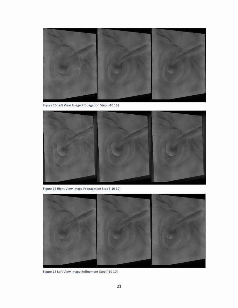
Figure 16 Left View Image Propagation Step [-10 10]
Figure 17 Right View Image Propagation Step [-10 10]
Figure 18 Left View Image Refinement Step [-10 10]

22
Figure 19 Right View Image Refinement Step [-10 10]
Figure 20 (a) Left View Image Disparity Map [-10 10]; (b) Right View Image Disparity Map [-10 10]
(a) (b)

23
2.2.3.3. Disparity Test Value [-30 30]
(b) (a)
Figure 21 (a) Left View Image Initialization Step [-30 30]; (b) Right View Image Initialization Step [-30 30]
Figure 22 Left View Image Propagation Step [-30 30]

24
Figure 23 Right View Image Propagation Step [-30 30]
Figure 25 Right View Image Refinement Step [-30 30]
Figure 24 Left View Image Refinement Step [-30 30]

25
From the figures shown above it can be clearly seen that the results, when choosing disparity
values to be -10 10, are of the better quality than the rest of the two-other set of images. Also
choosing -30 30 yields the worst result amongst the three sets. These results directly affect the
next step of the approach which is point cloud generation. If the disparity maps are not well
defined or have a significant amount of noise in them then the resulting point cloud is a noisy
mesh as well.
These results were achieved using the GPU implementation of the Patchmatch Stereo
algorithm. The same results can also be achieved by using the CPU version but it is highly time
consuming. Table 2 Comparison Between Computational Time Required by CPU and GPU
Implementation of the Patchmatch Stereo Algorithm provides the comparison in running time
(b) (a)
Figure 26 (a) Left View Image Disparity Map [-30 30]; (b) Right View Image Disparity Map [-30 30]

26
between the CPU and GPU implementation of the Patchmatch Stereo algorithm for different
SEM images.
Table 2 Comparison Between Computational Time Required by CPU and GPU Implementation of the Patchmatch Stereo Algorithm; http://selibcv.org/3dsem/; https://www.sciencedirect.com/science/article/pii/S0968432817303128
SEM Dataset CPU Implementation
GPU Implementation
Diatom Frustule 12895.30seconds/ 214.922minutes/
3.582hours
85.61seconds/ 1.426minutes
Hexagon TEM Copper Grid
13401.59seconds/ 223.359minutes/
3.723hours
83.75seconds/ 1.395minutes
Pollen
12636.05seconds/ 210.601minutes/
3.510hours
83.83seconds/ 1.397minutes
Tapetal Cell of Arabidopsis Thaliana
15009.24seconds/ 250.154minutes/
4.169hours
84.64seconds/ 1.444minutes
Pollen Grain from Brassica Rapa
12596.33seconds/ 209.939minutes/
3.499hours
85.55seconds/ 1.426minutes
Pseudoscorpion
12601.89seconds/ 210.0315minutes/
3.501hours
82.86sec/ 1.381minutes
Anther
13341.91seconds/ 222.365minutes/
3.706hours
86.03sec/ 1.434minutes

27
All the SEM images used here were of the same resolution 640x480 for the sake of fairness of
comparison. The disparity values were set to -10 10 for every stereo pair of every dataset. It is
clearly seen that the GPU implementation is much faster than the CPU implementation. The
computational time difference between the two implementations is huge. It takes the CPU
several hours to compute whereas the GPU does the same computation in less than a couple of
minutes. If the resolution of the images were to be higher than the one being used or if the
disparity values were set to a higher range the computational time would also increase multiple
folds specially for the CPU implementation.
The next step is to generate dense point cloud and from that constructing the
3D surface model. To achieve a much better-quality construction the approach adds the feature
of point cloud registration. This not only provides better viewing angles for the constructed 3D
model but also a much denser surface reconstruction which is the main objective of this
research.
2.2.4. Point Cloud Generation and Registration
The results from the previous step are crucial for the point cloud generation. The quality of the
point cloud depends on the correctness of the rectification of the stereo images and the
disparity map generated by the Patchmatch algorithm. Once the depth map has been received
the point cloud can generated using the rectified image that was used as input to the
Patchmatch algorithm. An important parameter here is the rotation angle which the user must
provide. Usually if the SEM images are taken by the user then the rotation angle is known and
that helps in achieving relatively more accurate results.

28
This 3D reconstruction is done by using the resulting depth map of the disparity value
test set -10 10. Once the 3D construction is done and high detail result is achieved we can move
to the next step of registration. But before that the we must generate multiple cloud points
from different images of the same dataset. This means that the approach described until now
has to be implemented several times (at least 2 times) since registration can be performed on
Figure 27 3D Surface Reconstruction of Pseudoscorpion SEM Stereo Pair

29
at least 2 set of point clouds. From Figure 28 Sparse 3D Reconstructed Pseudoscorpion Surface
below it is seen that from a single stereo pair the reconstruction can be sparse.
This structure is missing details and geometry which is crucial when the interest lies in
observing the true shape of the sample. This is where point cloud registration helps and
overcomes this obstacle. Point cloud registration is basically using transformation and rotation
tools and fitting the two points clouds in such a manner that the key points match with high
accuracy. Figure 29 Dense 3D Surface of Pseudoscorpion using Point Cloud Registration shows
how point cloud registration overcomes this obstacle and provides a much better 3D model to
work with.
Figure 28 Sparse 3D Reconstructed Pseudoscorpion Surface

30
2.3. Results
Figure 29 Dense 3D Surface of Pseudoscorpion using Point Cloud Registration
Figure 30 Hexagon TEM Copper Grid Dataset http://selibcv.org/3dsem/

31
Figure 31 Reconstructed 3D Model without Point Cloud Registration Hexagon TEM Copper Grid Dataset
Figure 32 Reconstructed 3D Model with Point Cloud Registration Hexagon TEM Copper Grid Dataset

32
Figure 33 Pollen Grain from Brassica Rapa Dataset http://selibcv.org/3dsem/
Figure 34 Reconstructed 3D Model without Point Cloud Registration Pollen Grain from Brassica Rapa Dataset

33
Figure 35 Reconstructed 3D Model with Point Cloud Registration Pollen Grain from Brassica Rapa Dataset
Figure 36 TEM Copper Grid Dataset http://selibcv.org/3dsem/

34
Figure 37 Reconstructed 3D Model without Point Cloud Registration Pollen Grain from TEM Copper Grid Dataset
Figure 38 Reconstructed 3D Model with Point Cloud Registration Pollen Grain from TEM Copper Grid Dataset

35
2.4. Conclusion
The results shown do provide a denser and a much more complete view of the specimen as
compared to the traditional 2 image 3D reconstruction. The results are not only dense but also
provides more detail and information about the structure and shape of the SEM micrograph.
Even though the results are better than before, this approach has its limitations. Since the
approach works locally, that is, it generates the point clouds for every pair of stereo images
independently, the errors and noise generated in each point cloud is accumulated in the final
result when all the point clouds are registered.
To tackle this problem a global approach method is discussed in the next chapter which
instead of working on 2 images at a time, works on the entire data set to find the matches
between the images and computing the correspondence between these images within a
dataset.

36
Chapter 3
Global Approach: Regard3D
3.1. Introduction to Regard3D
Regard3D is a structure-from-motion program. That means, it can create 3D models from
objects using a series of photographs taken of this object from different viewpoints. The
photographs provided as the input must follow this criterion for best possible results:
• Image must be JPEG.
• The focal length as well as the sensor size of the imaging device (for at least some
pictures) must be known. This means that:
o EXIF (metadata) must be present. This provides focal length and camera’s
make and model.
o The imaging device (camera) used must be in Regard3D’s database.
• Higher the resolution better the resulting reconstruction.
• The photographs should provide a complete view of the object. Any part of the
object not visible in more than three pictures will be excluded from the resulting 3D
model.
Classic A-KAZE (more precise but slower) and Fast A-KAZE (faster but slightly less good key-
points get detected) are two key-point detectors that are used in this approach.

37
3.2. KAZE Algorithm
KAZE is a multiscale 2D feature detection and description algorithm in nonlinear scale
spaces. Previous approaches detect and describe features at different scale levels by building or
approximating the Gaussian scale space of an image. However, Gaussian blurring does not
respect the natural boundaries of objects and smooths to the same degree both details and
noise, reducing localization accuracy and distinctiveness. In contrast, KAZE detects and
describes 2D features in a nonlinear scale space by means of nonlinear diffusion filtering. This is
done by blurring locally adaptive to the image data, reducing noise but retaining object
boundaries, obtaining superior localization accuracy and distinctiveness. Even though the
features are somewhat more expensive to compute than SURF due to the construction of the
nonlinear scale space, but comparable to SIFT, the results reveal a step forward in performance
both in detection and description against previous state-of-the-art methods. The algorithm
used in this particular approach is the sped-up version of the KAZE algorithm. It is known as
Accelerated KAZE or A-KAZE.
3.3. A-KAZE
A-KAZE or Accelerated KAZE uses a mathematical framework called Fast Explicit Diffusion
(FED) to dramatically speed-up the nonlinear scale space computations. A-KAZE achieves
comparable results to KAZE (in some datasets) while being much faster than the KAZE.

38
3.4. Obtaining a 3D Model
To obtain a 3D model, the following steps are performed:
3.4.1. Feature Point Detection
For each image, features also called key-points are detected. Features are points in an
object that have a high probability to be found in different images of the same object,
for example corners, edges etc. Regard3D uses A-KAZE for this purpose.
For each feature, a mathematical descriptor is calculated. This descriptor has the
characteristic that descriptors of the same point in an object in different images (seen
from different viewpoints) is similar. Regard3D uses Local Intensity Order Pattern (LIOP)
for this purpose.
3.4.2. Key-point Matching
The descriptors from different images are matched and geometrically filtered. The result
of this step is a collection of matches between each image pair.
Now "tracks" are calculated. For each feature that is part of a match in an image
pair, it is searched also in other images. A track is generated from features if these
features satisfy some conditions, for example a track is seen in at least 3 images.
3.4.3. Triangulation
The next step is the triangulation phase. All the matches of all the image pairs are used
to calculate:
o The 3D position and characteristic of the "camera", i.e. where each image was
shot and the visual characteristics of the camera.

39
o The 3D position of each "track" is calculated
3.4.4. Densification
The result of the triangulation phase is a sparse point cloud. To obtain a denser point
cloud ("densification"), several algorithms can be used.
3.4.5. Surface Generation
• The last step is called "Surface generation". The point clouds are used to generate a
surface, either with colored vertices or with a texture.

40
3.5. Pipeline
Input Dataset
• Input a set of images.
Compute Matches
• detect keypoints in each image and match them with keypoints from other images. This is done using A-KAZE.
Triangulation
• The 3D position and characteristic of the camera (where each image was shot) is calculated.
Densification
• The triangulated point cloud is rather sparse, it is difficult to make out the original object. The point cloud is densified so a surface can be constructed.
Surface Generation
• Since it is still a point cloud (a set of 3D points with color), a surface that connects (most of) these points is constructed.

41
3.6. Results
3.6.1. Dataset 1: Kermit
Figure 39 Kermit Dataset 11 Images Montage https://www.gcc.tu-darmstadt.de/home/proj/mve/

42
Figure 40 Matching Results from Kermit Dataset
Figure 41 Dense Point Cloud Generation from Triangulated Points Kermit

43
Figure 42 Generated Surface from 11 Images Kermit Dataset

44
Figure 43 Der Hass Dataset 79 Images Montage https://www.gcc.tu-darmstadt.de/home/proj/mve/
3.6
.2.
Dataset 2
: Der H
ass

45
Figure 44 Matching Results From Der Hass Dataset
Figure 45 Dense Point Cloud Generation from Triangulated Points Der Hass

46
Figure 46 Generated Surface from 79 Images Der Hass Dataset

47
The results shown above were generated using Regard3D running on a system with
specifications as follows:
• Processor: Intel® Core™ i5-75300HQ CPU @ 2.50GHz 2.50GHz
• RAM: 8.00 GB
From the table provided below, the time it takes for each step to complete can be seen as well
as the total time it takes from finding putative matches to generation of the surface with
textures.
Table 3 Step by Step Running Time for Each Dataset
Dataset Number of
Images
Compute Matches
Triangulation Create Dense
Pointcloud
Generate Surface
Total Time
Kermit 11 7.889 sec 2.293 sec 113.227 sec 218.591 sec 342sec
Der Hass
79 475.585sec 59.750sec 1111.190sec 1158.187sec 2804.712sec
Both the datasets used were downscaled to the same image resolution of 640x480 for the sake
of relatively faster running time and fair comparison. The settings that were used for each step
were set for achieving maximum level detail in the final 3D generated surface model. As shown
in Table 3 Step by Step Running Time for Each Dataset the total time it took for Kermit dataset
which consists of 11 images is 342 seconds or 5 minutes and 42 seconds. As for the Der Hass
dataset which consisted of 79 images the total time required to generate the 3D surface was
2804.712 seconds or 46 minutes and 44.712 seconds.

48
3.7. Other Low Detail 3D Reconstructions
Figure 47 Low Detail 3D Model Reconstruction of Objects From 3 Images
Figure 48 Low Detail 3D Model Reconstruction of Human Face with 30 Images

49
3.8. Conclusion
The approach demonstrated above is a general/global 3D reconstruction approach. It can
be used to generate 3D model surfaces from any given set of images as long as the camera
parameters are known to the user. This provides nicely detailed geometry and textures with
fine details. As mentioned in the requirements the higher the input image quality the higher the
quality of the resulting 3D model will be. The difference in quality can also be seen from
comparing Figure 42 Generated Surface from 11 Images Kermit Dataset, Figure 46 Generated
Surface from 79 Images Der Hass Dataset, Figure 47 Low Detail 3D Model Reconstruction of
Objects From 3 Images and Figure 48 Low Detail 3D Model Reconstruction of Human Face From
30 Images.
Even though the results from this general 3D modeling approach are promising and look
good, the actual goal to achieve is 3D surface reconstruction of SEM images is not yet
achievable using this approach. Since the intrinsic camera parameters such as the camera’s
focal length and sensor width are not known, it is not possible to add these values to the
camera database for Regard3D. Thus, some modifications and enhancements are to be made
before it can be done.

50
Chapter 4
Conclusions
4.1. Conclusions and Future Work
In this thesis we surveyed different approaches for the 3D surface reconstruction. We
discussed the multi-view approach which takes only two images as input at a time. This
approach included several steps such as image rectification, using Patchmatch Stereo’s GPU
implementation and point cloud registration. The approach is useful when dealing with SEM
images as can be seen from the figures in the Chapter 2. Since a 3D reconstruction from only
two images does not always necessarily provide enough detail and texture, thus the 3D view
remains incomplete. With the approach discussed in Chapter 2 we can provide multiple images
as input (two at a time) and then generate multiple point clouds for the surface reconstruction.
But this pose another obstacle that no view is fully complete view of the specimen under
observation.
Point Cloud Registration being the answer to the problem, is used in this thesis to merge
those multiple point clouds for the same specimen and creating one complete 3D surface. This
registration technique helps not only to provide a more complete view of the specimen but also
adds to missing points in other point clouds. During the generation of point clouds some detail
in geometry or texture is sometimes left out. This may happen due to faulty feature point
detection or some accuracy error during the Patchmatch procedure or can also be because of
the noise generated at any given step. With point cloud registration we overlap and fit the

51
feature points in such a way that it fills these holes and provides a view with small error and
more completeness in structure.
Point cloud generation from a pair of images and then registering them is still a local
approach to solving the problem thus any error generated in the point cloud generation will
accumulate when registering multiple point clouds. This can sometimes lead to results that are
not desired and are noisy rather than complete.
To overcome this problem, we discussed the global approach using Regard3D and
showed various results generated by the approach. The results were promising in terms of
details and large area reconstruction when the intrinsic camera parameters are known. The
approach used the Accelerated KAZE algorithm for the feature point extraction and
correspondence between the images. It also had multiple libraries backing it up for the purpose
of triangulation and surface reconstruction as well as point cloud creation. The end results were
impressive but this approach was not quite useful when applied on images whose EXIF or
camera details were not known specifically with the SEM images datasets.
Though this is an obstacle for now, but it can be solved by designing such programs that
can compute the parameters required by the global approach. With the focal length and
rotation angle known this approach can be applied not only to any point and shoot camera but
SEM micrographs as well thus providing a complete view (ideally 360-degrees).
Not only this but nowadays much work has been done in the field of computer vision for
integrating machine learning/deep learning techniques to the algorithms. This not only
improves the overall functionality of the program but also enhances the efficiency and

52
effectiveness. This new technology used along with the high-power GPUs can revolutionize the
field of computer vision by speeding up the processes and providing high quality results.

53
References
3D SEM. (2015). Retrieved from http://selibcv.org/3dsem
A. P. Tafti, A. B. Kirkpatrick, J. D. Holz, H. A. Owen, & Zeyun Yu. (2015). 3dsem: A 3d microscopy
dataset. Elsevier.
A. P. Tafti, A. B. Kirkpatrick, Z. Alavi, A. Owen, & Zeyun Yu. (2015). Recent advances in 3d sem
surface reconstruction.
A. P. Tafti, A. Baghaie, A. B. Kirkpatrick, J. D. Holz, H. A. Owen, R. M. DSouza, & Zeyun Yu.
(2016). A comparative study on the application of sift, surf, brief and orb for 3d surface
reconstruction of electron microscopy images. Computer Methods in Biomechanics and
Biomedical Engineering: Imaging & Visualization.
A. P. Tafti, J. D. Holz, A. Baghaie, H. A. Owen, M. M. He, & Zeyun Yu. (2016). 3dsem++: Adaptive
and intelligent 3d sem surface reconstruction (Vol. 87). Elsevier.
A. Zolotukhin , I. Safonov, & K. Kryzhanovskii. (2013). 3d reconstruction for a scanning electron
microscope. Pattern recognition and image analysis.
Ahmadreza Baghaie, & Heather A. Owen. (2017, September 11). Stereo Scanning Electron
Microscopy Dataset.
Ahmadreza Baghaie, Ahmad Pahlavan Tafti, Heather A. Owen, Roshan M. D’Souza, & Zeyun Yu.
(2017, April 6). Three-dimensional reconstruction of highly complex microscopic
samples using scanning electron microscopy and optical flow estimation.
B. Zitova, & J. Flusser. (2003). Image registration methods: a survey. Image and vision
computing.
Baghaie, A. (2016). Study of Computational Image Matching Techniques: Improving Our View of
Biomedical . Milwaukee.
Baghaie, A., C. Z., A. B., H. A., H. C., R. M., & Z. Y. (2017, December). Slanted support window-
based stereo matching for surface reconstruction of microscopic samples.
Caroline A Schneider, Wayne S Rasband, & Kevin W Eliceiri. (2012, June 28). NIH Image to
ImageJ: 25 years of image analysis. Nature Methods.
CloudCompare. (n.d.). Retrieved from http://www.cloudcompare.org/
Dr. Michael D. Abramoff, Dr. Paulo J. Maghalhaes, & Dr. Sunanda J. Ram. (2004). Image
Processing with ImageJ.
Herbert Bay, Andreas Ess, Tinne Tuytelaars, & Luc Van Gool. (2008). Speeded-Up Robust
Features (SURF).

54
Herbert Bay, Tinne Tuytelaars, & Luc Van Gool. (2006). SURF: Speeded Up Robust Features.
Springer.
Hiestand, R. (2015). Regard3D. Retrieved from http://www.regard3d.org
ImageJ. (1997-2016). Retrieved from https://imagej.nih.gov/ij/
J Bernal, F Vilarino, & J Sánchez. (2010). Feature detectors and feature descriptors: where we
are now. 8193.
K. M. Lee, & C.-C. J. Kuo. (1993). Surface reconstruction from photometric stereo images.
Michael Bleyer, Christoph Rhemann, & Carsten Rother. (n.d.). PatchMatch Stereo - Stereo
Matching with Slanted Support Windows.
P. Cignoni, M. Callieri, M. Corsini, M. Dellepiane, F. Ganovelli, & G. Ranzuglia. (2008). MeshLab:
an Open-Source Mesh Processing Tool.
SeLibCV. (n.d.). Retrieved from http://selibcv.org/
Simon Fuhrmann, Fabian Langguth, & Michael Goesele. (2014). MVE – A Multi-View
Reconstruction Environment.
Tafti, A. P. (2016). 3D SEM Surface Reconstruction: An Optimized, Adaptive, and Intelligent
Approach.
Tafti, A., Kirkpatrick, A., Owen, H., & Yu, Z. (2014). 3D Microscopy Vision Using Multiple View
Geometry and Differential Evolutionary Approaches. In Advances in Visual Computing.
Springer.
Velasco, E. (2013). Scanning Electron Microscope (SEM) as a means to determine dispersibility.
Vernon-Parry, K. (2000). Scanning electron microscopy: an introduction. Elsevier.