1

3D View-Invariant Face Recognition Using a HierarchicalPose-Normalization Strategy

____________________________________________________________

Authors: Martin D. Levine and Ajit RajwadeCenter of Intelligent Machines,

Room 410, 3480 University Street,McConnell Engineering Building,

McGill University,Montreal, H3A 2A7,

Canada.

Address: Same as above.

Email addresses: Levine@cim.mcgill.ca, ajitvr@cim.mcgill.ca

Corresponding Author: Martin D. Levine

2

Abstract

Face recognition from 3D shape data has been proposed as a method of biometric identificationas a way of either supplementing or reinforcing a 2D approach. This paper presents a 3D facerecognition system capable of recognizing the identity of an individual from a 3D facial scan inany pose across the view-sphere, by suitably comparing it with a set of models (all in frontalpose) stored in a database. The system makes use of only 3D shape data, ignoring texturalinformation completely. Firstly, we propose a generic learning strategy using support vectorregression [2] to estimate the approximate pose of a 3D head. The support vector machine (SVM)is trained on range images in several poses belonging to only a small set of individuals and is ableto coarsely estimate the pose of any unseen facial scan. Secondly, we propose a hierarchical two-step strategy to normalize a facial scan to a nearly frontal pose before performing any recognition.The first step consists of either a coarse normalization making use of facial features or the genericlearning algorithm using the SVM. This is followed by an iterative technique to refine thealignment to the frontal pose, which is basically an improved form of the Iterated Closest PointAlgorithm [8]. The latter step produces a residual error value, which can be used as a metric togauge the similarity between two faces. Our two-step approach is experimentally shown tooutperform both of the individual normalization methods in terms of recognition rates, over avery wide range of facial poses. Our strategy has been tested on a large database of 3D facialscans in which the training and test images of each individual were acquired at significantlydifferent times, unlike all except one of the existing 3D face recognition methods.

Keywords: 3D face recognition; support vector regression; iterated closest point; 3D poseestimation; pose normalization; residual error

Acknowledgements: The authors would like to thank National Sciences and EngineeringResearch Council, Canada for their financial assistance.

3

List of Figures:

Figure 1:Sample Faces from the Freiburg Database 14

Figure 2: Faces from the Notre Dame Database 14

Figure 3: A Few Cropped Models from the Notre Dame database 20

Figure 4: Typical corresponding cropped probe images from the Notre DameDatabase

21

Figure 5: Residual error between different images of the same persons 24

Figure 6:Residual error values between different images of different persons 24

Figure 7: Residual error histogram for images of the same (red) and different(green) people shown together for comparison

25

Figure 8: Recognition rate versus image size 27

Figure 9: Recognition rate versus number of training images 28

Figure 10: Two scans of the same person with different facial expressions 28

Figure 11: Removal of non-rigid regions of the face (region below the four darklines)

29

4

List of Tables

Table 1:Results of Pose Estimation 15

Table 2:Recognition rates with ICP, ICP-variant and LMICP 23

Table 3:Recognition rates with ICP and the ICP-Variants afterapplying the feature-based method as an initial step

23

Table 4:Recognition rates with ICP and ICP Variant after applyingSVR as the initial step

23

5

1. Introduction

Owing to heightened security concerns during the past decade, face recognition hasemerged as an important method of biometric authentication. Traditional methods ofrecognizing the identity of individuals use 2D facial images. However, 2D images of anobject are known to be inherently sensitive to incident illumination. Thus images of oneand the same individual under different lighting conditions tend to differ to a greaterextent than those of different individuals under the same lighting conditions [1]. Apossible way to circumvent this difficulty is the employment of a sensor, which gathersdata in a manner insensitive to visible light. One such sensor is a 3D range scanner,which measures the actual 3D shape of the face and so is inherently invariant to changesin illumination.

Face recognition systems are also very sensitive to variation in facial pose. A robustsystem should be able to recognize individuals across a very large range of poses, ideallythe entire view-sphere. Geometric normalization for pose variations is certainly simplergiven the 3D shape of a person’s head, than from the 2D texture image. Nonetheless,robustly dealing with pose variations remains a major issue even in face recognitionsystems that use 3D data.

In this paper, we outline a hierarchical strategy to normalize the 3D scan of a person’sface (in any pose across the entire view-sphere) to a closely frontal view. Our hierarchicalstrategy consists of an approximate normalization using support vector regression (SVR)[2] followed by a refined normalization using an improved variant of an existing surface(or curve) registration method, the “iterated closest point” (ICP) algorithm [8]. To test theefficacy of the combined strategy, we take an ensemble of 3D facial scans belonging toseveral individuals, originally in several different views, and normalize them using ourtechnique. Thereafter, we compare these scans with a database containing frontal 3Dscans of the same individuals and ascertain the recognition rates.

We report a recognition rate of 91.5% on the Notre Dame database for the case of asingle 3D training image. We also quantify the variation in recognition rates with respectto increasing pose-difference between training and test images, To the best of ourknowledge, this is the first attempt to systematically study the effect of pose variation onthe 3D face recognition rate. Our two-step pose-normalization method is shown to bestable over a large range of views across the entire view-sphere (inclusive of profileviews), unlike existing studies which have reported recognition rates only on near-frontalhead poses ([10], [11], [12], [14], [16], [17], [18], [20], [22], [23]). Both the work in [17]and this paper represent the largest studies done on 3D face recognition so far.Additionally, unlike most existing systems (with the sole exception of [17]), our approachhas been tested on a database in which the time interval between the acquisition oftraining and test images is significant. In comparison to [17], we report a slightly lowerrecognition rate on the same database. However, it should be noted that the approach in[17] requires considerable manual intervention, whereas the method described in thispaper is fully automated.

6

This paper is organized as follows. Section (2) briefly reviews the existing literature in3D face recognition. Section (3) presents a bird’s eye view of the approach discussed inthe paper. Thereafter, in section (4), we proceed to describe our strategy in greater detail,beginning with a brief discussion of the theory of support vector machines and theirapplication to facial pose estimation from range data. In section (5), we explain the needfor further refinement of the pose estimate and give a detailed description of ICP and itsmerits and demerits. We also describe a variant of ICP that uses simple heuristics toimprove the registration performance (in terms of recognition accuracy). Severalexperimental results on a large face database (obtained from Notre Dame University [17])are presented in section (6) along with detailed discussions. Finally, section (7) presentsthe conclusions along with pointers to possible future work.

2. Background

Heretofore, not many papers have been published on 3D face recognition. The existingliterature can be divided into different categories based on the approach followed. Theseinclude 3D face recognition methods employing principal components analysis (PCA),methods that represent faces as vectors of specific features, methods that use pointsignatures and methods that use the iterated closest point (ICP) algorithm. This sectionbriefly reviews these approaches and their reported results, followed by a short critique.

(2.1) Methods Using PCA

Principal Components Analysis (PCA) was first used for the purpose of 2D facerecognition in the paper by Turk and Pentland [9]. The technique has been applied to 3Dface recognition by Hesher and Srivastava [10]. Their database consisted of 222 range-images of 37 different people. The different images of one and the same person have 6different facial expressions. The range images are normalized for pose changes by firstdetecting the nasal bridge and then aligning it with the Y-axis. An eigenspace is thencreated from the “normalized” range-images and used to project the images onto a lowerdimensional space. Using exactly one gallery image per person, a face recognition rate of83% was obtained.

PCA has also been used by Tsalakanidou et al [11] on a set of 295 frontal 3D images,each belonging to a different person. They chose one range image each of 40 differentpeople to build an eigenspace for training purposes. Their test set consisted of artificiallyrotated range images of all the 295 people in the database, varying the angle of rotationaround the Y-axis from 2 to 10 degrees. For the 2-degree rotation case, they claim arecognition rate of 93%, but this rate drops to 85% for rotations larger than 10 degrees.

Yet another study using PCA on 3D data has been reported by Achermann et al [12].They have used the PCA technique to build an eigenspace out of 5 poses each of 24different people. Their method has been tested on 5 different poses each of the sameperson but the poses of the selected test images seem to lie between the different training

7

poses.1 The authors report a recognition rate of 100% on their data set using PCA with 5training images per person. They have also applied the method of Hidden MarkovModels on exactly the same data set and report recognition results of 89.17%.

Chang et al [17] report the largest study on 3D face recognition to date, which is based ona total of 951 range images of 277 different people. Using a single gallery image perperson, and multiple probes, each taken at different time intervals as compared to thegallery, they obtained a face recognition rate of 92.8% by performing PCA using just theshape information. They have also examined the effect of spatial resolution (in X, Y andZ directions) on the accuracy of recognition. However, they actually perform manualfacial pose normalization by aligning the line joining the centers of the eyes with the X-axis, and the line joining the base of the nose and the chin with the Y-axis. Obviously,manual normalization is not feasible in a practical system, besides being prone to humanerror in marking feature points.

(2.2) Feature-based methods

Surface properties such as maximum and minimum principal curvatures allowsegmentation of the surface into regions of concavity, convexity and saddle points, andthus offer good discriminatory information for object recognition purposes. Tanaka et al[14] calculate the maximum and minimum principal curvature maps from the depth mapsof faces. From these curvature maps, they extract the facial ridge and valley lines. Theformer are a set of vectors that correspond to local maxima in the values of the minimumprincipal curvature. The latter are a set of vectors that correspond to local minima in thevalues of the maximum principal curvature. From the knowledge of the ridge and valleylines, they construct extended Gaussian images (EGI) for the face by mapping each of theprincipal curvature vectors onto two different unit spheres, one for the ridge and the otherfor the valley lines. Matching between model and test range images is performed usingFisher’s spherical correlation [15], a rotation-invariant similarity measure, between therespective ridge and valley EGI. This algorithm has been tested on only 37 range images,with each image belonging to a different person and 100%2 accuracy has been reported.However, extraction of the ridge and valley lines requires the curvature maps to bethresholded. This is a clear disadvantage because there is no explicit rule to obtain anideal threshold, and the location of the ridge and valley lines are very sensitive to thechosen value.

Lee and Milios [20] obtain convex regions from the facial surface using curvaturerelationships to represent distinct facial regions. Each convex region is represented by anEGI by performing a one-to-one mapping between points in those regions and points onthe unit sphere that have the same surface normal. The similarity between two convexregions is evaluated by correlating their Extended Gaussian images. To establish thecorrespondence between two faces, a graph-matching algorithm is employed to correlatethe set of only convex regions in the two faces (ignoring the non-convex regions). It isassumed that the convex regions of the face are more insensitive to changes in facial 1 No specific data are provided in this paper.2 See Section 2.5 for a detailed discussion of results reported in other publications.

8

expression than the non-convex regions. Hence their method has some degree ofexpression invariance. However, they have tested their algorithm on range images of only6 people and no results have been explicitly reported.

Feature-based methods aim to locate salient facial features such as the eyes, nose andmouth using geometrical or statistical techniques. Commonly, surface properties such ascurvature are used to localize facial features by segmenting the facial surface intoconcave and convex regions and making use of prior knowledge of facial morphology[16], [18]. For instance, the eyes are detected as concavities (which correspond topositive values of both mean and Gaussian curvature) near the base of the nose.Alternatively, the eyebrows can be detected as distinct ridgelines near the nasal base. Themouth corners can also be detected as symmetrical concavities near the bottom of thenose. After locating salient facial landmarks, feature vectors are created based on spatialrelationships between these landmarks. These spatial relationships could be in the form ofdistances between two or more points, areas of certain regions, or the values of the anglesbetween three or more salient feature-points. Gordon [16] creates a feature-vector of 10different distance values to represent a face, whereas Moreno et al [18] create an 86-valued feature vector. Moreno et al [18] segment the face into 8 different regions and twodistinct lines, and their feature-vector includes the area of each region and the distancebetween the center of mass of the different regions as well as angular measures. In both[16] and [18], each feature is given an importance value or weight, which is obtainedfrom its discriminatory value as determined by Fisher’s criterion [19]. The similaritybetween gallery and probe images is calculated as the similarity between thecorresponding weighted feature-vectors. Gordon [16] reports a recognition rate of 91.7%on a dataset of 25 people, whereas Moreno et al [18] report a rate of 78% on a dataset of420 range images of 60 individuals in two different poses (looking up and down) andwith five different expressions. A major disadvantage of these methods is that thelocation of accurate feature-points (as well as points such as centroids of facial regions) ishighly susceptible to noise, especially because curvature is a second derivative. Thisleads to errors in the localization of facial features. The errors are further increased witheven small pose changes that can cause partial occlusion of some features, for instancedownward facial tilts that partially conceal the eyes. Hence the feature-based methodsdescribed in [16] and [18] lack robustness.

(2.3) Methods Using Point Signatures

The concept of point signatures was discovered by Chua and Jarvis and was used for thepurpose of robust object recognition in [21]. It was extended to expression-invariant 3Dface recognition by Chua, Han and Ho [22]. In the latter, the facial surface is treated as anon-rigid surface. A heuristic function is first used to identify and eliminate the non-rigidregions on the two facial surfaces (further details in [22]). Correspondence is establishedbetween the rigid regions of the two facial surfaces by means of correlation between therespective point signature vectors and other criteria such as distance, and finally theoptimal transformation between the surfaces is estimated in an iterative manner. Despiteits advantages, this method has been tested on images of only six different people, withfour range images of different facial expressions for each of the six persons. Another

9

disadvantage is that the registration achieved by this method is not very accurate3 (asreported in [22]) and requires a further refinement step such as ICP. This two-stepprocedure contains two iterative steps and is computationally very expensive.

The concept of point signatures has also been used for face recognition in recent work byWang, Chua and Ho [23]. They manually select four fiducial points on the facial surfacefrom a set of training images and calculate the point signatures over 3 by 3neighborhoods surrounding those fiducial points (i.e., 9 point signature vectors). Thesesignature vectors are then concatenated to yield a single feature vector. The selectedfiducial points include the nasal tip, the nasal base and the two outer eye corners. Aseparate eigenspace is built from the point signatures in the 3 by 3 neighborhoodsurrounding each fiducial point in each range image. Thus, four different eigenspaces areconstructed in total. To locate the corresponding four fiducial points in a test rangeimage, point signatures are calculated for 3 by 3 neighborhoods surrounding each pixel inthe image and represented by a single vector. The distance from feature space (DFFS)value is calculated between the vector at each pixel on the test face and the foureigenspaces created during training. The fiducial points correspond to those pixels atwhich the DFFS value with respect to the appropriate eigenspace is minimal. For facematching, classification is performed using support vector machines [2], with the inputconsisting of the pixel signature vectors in the 3 by 3 neighborhoods surrounding the fourfiducial points. The maximum recognition rate with three training images and three testimages per person is reported to be around 85%. The different images collected for eachperson show some variation in terms of facial expression. The authors do not specify theeffect of important parameters such as the radius of the sphere required for calculating thepoint signatures. Furthermore, their approach takes into account data at only four fiducialpoints on the surface of the face. This seems to be inadequate from the point of view ofrobust facial discrimination, as it tends to ignore several important regions of the face.They have also not given any statistical analysis of errors in localization of the facialfeature points and the effect on recognition accuracy.

(2.4) Methods Using ICP

Lu, Colbry and Jain have used an ICP-based method for facial surface registration in [25]and [26]. They employed a feature-based method followed by a hybrid ICP algorithmalternating in successive iterations between the method proposed by Besl & McKay [8]and that proposed by Chen and Medioni [24]. In this way they are able to make use of theadvantages of both algorithms: the greater speed of the Besl and McKay [8] techniqueand the greater accuracy of the method of Chen and Medioni [24]. Their hybrid ICPalgorithm has been tested on a database of 18 individuals with frontal gallery and probeimages involving pose and expression variations. A probe image is registered with eachof the 18 gallery images, and the gallery image giving the lowest residual error is the onethat is considered to be the best match. Using the residual error alone, they obtain a

3 No exact results are specified in [23].

10

recognition rate of 79.3%. This result is improved to 84% by incorporating additionaldata such as a shape index and texture4.

(2.5) Critique

Two important shortcomings in most existing 3D face recognition systems are worthmentioning. Firstly, apart from [17], none of the experiments described in this sectionspecify the time-span between the collection of the training and testing images for thesame person. It needs to be assumed, therefore, that the scans for each person were doneat the same sitting. The inclusion of sufficient time gaps between the collection oftraining and testing images is a vital component of the well-known FERET protocol forface recognition [13]. Likewise, none of the aforementioned papers has presented adetailed study of the effect of the increase in pose difference between gallery and probeimages on the recognition rate reported by the respective algorithms. Additionally, thetechniques described in the literature are designed to work only for those facial poses inwhich both eyes are clearly visible.

In this study, we use the same database as [17] and report a recognition result of 91.5%(as against their 92.8%). However, ours is a fully automated system, unlike the one in[17] which requires manual intervention for detection of salient feature-points.Additionally, we show results that quantify the effect of pose variation between probeand gallery images, and report results that are fairly stable across a wide range of posescovering the entire view-sphere. To the best of our knowledge, ours is the first attempt toperform such an investigation.

3. Overview

The aim of our system is to normalize for facial pose changes in a completely automatedmanner. Intuitively, feature-based methods that can reliably detect three distinct fiducialpoints on the face can be utilized for the purpose of pose alignment. Most of the priorresearch on 3D facial pose-normalization employs feature detectors to locate the twoinner eye corners and the nasal tip ([16], [17]). The actual alignment is performed usingprior knowledge of the spatial relationships between selected fiducial points on acanonical frontal face. For instance, the face is rotated in such a way that the line joiningthe two inner eye corners is aligned with the horizontal or X-axis, and the line that joinsthe nasal tip to the center of the line connecting the two inner eye corners, always has afixed orientation with the Y-axis. If the eye-corners and nasal tip are detected accurately,the face will be easily normalized to an exact frontal view. These methods have beenemployed in [16] with automated feature detection and in [17] with manual techniques.Given a set of normalized faces, a simple Euclidian distance comparison can act as areliable metric for recognition. However, these techniques cannot be employed for largepose variations across the view-sphere. For instance, in facial views with a large yaw 4 The recognition rate referred to here is for the case of the automated hybrid ICP algorithmapplied to range images without considering texture. See Table (1) in [25]. The column entitled“ICP hybrid, automatic, range-image only” states that the recognition rate is 79% [(63-13)/63].

11

rotation, several distinctive facial features, such as one of the eyes (and both the inner eyecorners) are obscured. Furthermore, feature-based methods lack robustness against noise,which is commonly found in range data and therefore the exact location of the individualpoints can be erroneous [18].

In this paper, we follow a different approach for pose normalization, which basicallystems from an interesting observation regarding facial pose variations: the faces ofdifferent individuals in similar poses show a marked similarity to one another, which canbe expressed in terms of the apparent 3D shape characteristics (or facial outlines) of aparticular pose. This is the primary motivation for the employment of machine learning torecognize the pose of an individual’s face. The specific technique used here is supportvector regression. A mathematical relationship is deduced between prototypical 3Dshapes in different poses and the poses themselves, the latter being quantified in terms ofthe angles of rotation around the Y- and X-axis (further details in [31]). Such a learningapproach has been used before by Gong et al [28] for pose estimation from 2D facialimages.

However, the learning algorithm cannot predict the exact angle from a 3D scan. Instead,we treat the angles found as coarse estimates and rotate the 3D facial scan to a roughlyfrontal face. Thereafter, we make use of the assumption of facial symmetry on either sideof the nasal ridge to correct for missing facial points. Finally, we utilize a robust variantof ICP [8] to refine the normalization by aligning the 3D scan to a pose as close aspossible to a perfectly frontal pose. The ICP algorithm (or its variant described in section(5) below) yields residual error values upon convergence, which can act as a reliablemetric for face recognition.

4. Pose Estimation Using Support Vector Machines In this section, we briefly describe the application of SVMs to pose estimation fromrange data, beginning with a note on the theory of support vector regression, andfollowed by an overview of the experimental method and summary of the results. Thereader is referred to [31] for detailed experimental results on facial pose estimation from3D shape information.

(4.1) Theory of Support Vector Regression

Support Vector Machines have emerged in recent times as a very popular data miningtechnique for applications such as classification [2], regression [4] and unsupervisedoutlier removal [5]. Consider a set of l input patterns denoted as x, with theircorresponding class labels, denoted by the vector y. A support vector machine obtains afunctional approximation given as bxwxf +Φ= )(.),( α , where Φ is a mapping functionfrom the original space of samples onto a higher dimensional space, b is a threshold, andα represents a set of parameters of the SVM. If y is restricted to the values –1 and +1, theapproximation is called support vector classification (SVC). If y can assume any validreal values, it is called support vector regression (SVR). By using a kernel function given

12

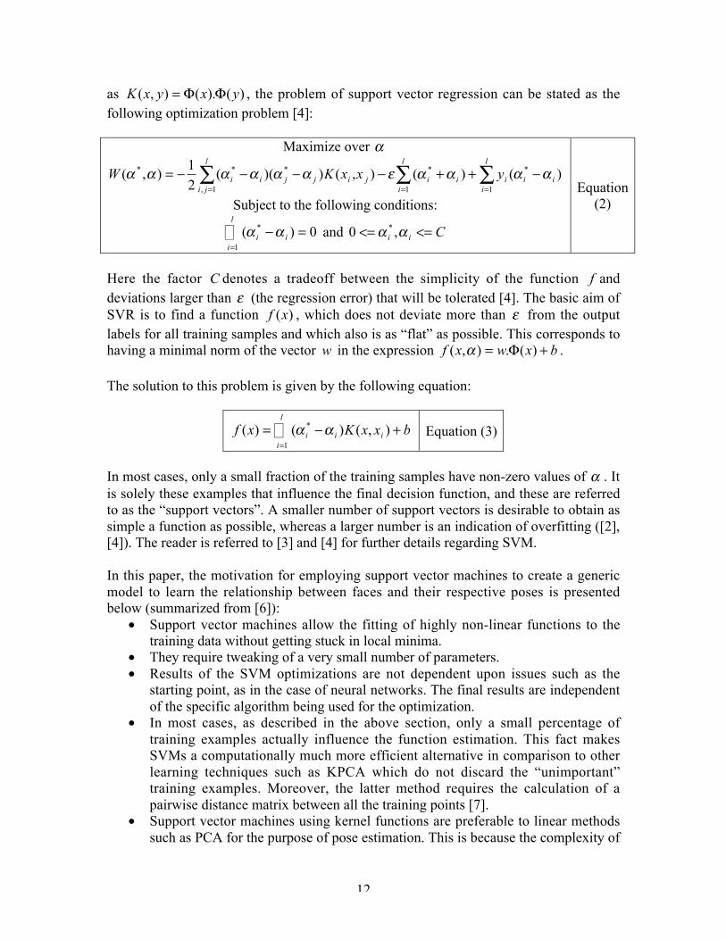
as )().(),( yxyxK ΦΦ= , the problem of support vector regression can be stated as thefollowing optimization problem [4]:

Maximize over α

∑∑∑===

−++−−−−=l

iiii

l

iiijijj

l

jiii yxxKW

1

*

1

**

1,

** )()(),()()(2

1),( ααααεαααααα

Subject to the following conditions:

0)(1

* =−�=

i

l

ii αα and Cii <=<= αα ,0 *

Equation(2)

Here the factor C denotes a tradeoff between the simplicity of the function f anddeviations larger than ε (the regression error) that will be tolerated [4]. The basic aim ofSVR is to find a function )(xf , which does not deviate more than ε from the outputlabels for all training samples and which also is as “flat” as possible. This corresponds tohaving a minimal norm of the vector w in the expression bxwxf +Φ= )(.),( α .

The solution to this problem is given by the following equation:

bxxKxfl

iiii +−= �

=

),()()(1

* αα Equation (3)

In most cases, only a small fraction of the training samples have non-zero values of α . Itis solely these examples that influence the final decision function, and these are referredto as the “support vectors”. A smaller number of support vectors is desirable to obtain assimple a function as possible, whereas a larger number is an indication of overfitting ([2],[4]). The reader is referred to [3] and [4] for further details regarding SVM.

In this paper, the motivation for employing support vector machines to create a genericmodel to learn the relationship between faces and their respective poses is presentedbelow (summarized from [6]):

• Support vector machines allow the fitting of highly non-linear functions to thetraining data without getting stuck in local minima.

• They require tweaking of a very small number of parameters.• Results of the SVM optimizations are not dependent upon issues such as the

starting point, as in the case of neural networks. The final results are independentof the specific algorithm being used for the optimization.

• In most cases, as described in the above section, only a small percentage oftraining examples actually influence the function estimation. This fact makesSVMs a computationally much more efficient alternative in comparison to otherlearning techniques such as KPCA which do not discard the “unimportant”training examples. Moreover, the latter method requires the calculation of apairwise distance matrix between all the training points [7].

• Support vector machines using kernel functions are preferable to linear methodssuch as PCA for the purpose of pose estimation. This is because the complexity of

13

the pose distribution of human faces under varying identity, expression orocclusion cannot be adequately modeled by linear methods [7].

It should also be noted that as the pose of a face is a continuous real-valued entity,regression is preferable to classification for the specific purpose of pose estimation.

(4.2) Description of the Data Set

The data for the pose estimation experiments in this paper were obtained from twosources. The first was the set of eigenvectors of manually aligned 3D shapes of humanfaces provided by the University of Freiburg [32]. As per the morphing method explainedin [32], 100 realistic-looking faces were generated by taking a linear combination of theprovided eigenvectors. All of these faces were in the exact frontal pose (0 degree headrotation about either axis). The second source of data was the facial range image databasefrom Notre Dame University [17], which contains near-frontal range images of 277individuals. The database contains considerable variations in hairstyles. A small subset ofthe range images in this database also contains slightly different expressions for one andthe same individual.

Since the faces in the Freiburg database were in the form of point-clouds, a surfacereconstruction step was necessary. This was performed using the “Power Crust SurfaceReconstruction Algorithm” [33]. To obtain training data in all possible poses for the poseestimation experiments, the facial surfaces were suitably projected onto different view-planes across the view-sphere. The range of poses considered was 0 to 90 degrees aroundthe Y-axis (yaw) and –30 to +30 degrees around the X-axis (tilt) in steps of 3 degrees.For the purpose of generating a good data set for pose estimation, the range images of theNotre Dame database were first manually aligned to closely frontal poses.5 For this thepositions of the eyes were marked manually, the line joining the eyes was aligned withthe horizontal and the nasal ridge was aligned with a fixed line, at 20 degrees with respectto the Y-axis. Range images that contained holes (missing data) were passed through asimple median filter. Portions of the images exterior to the facial contour were cropped.Different poses of each face were generated by projection onto different view-planes, asdescribed before.

Finally, all range images were resized to 160 by 160, taking care to preserve the aspectratio and padding an appropriate number of zeroes. A few faces from the Freiburg andNotre Dame databases, after the application of filtering and pre-processing techniques,are shown in Figure 1 and Figure 2.

5 It is important to note that this manual intervention was done only for training the poseestimation process. Using the latter functional relationship to estimate coarse pose, all recognitionexperiments reported in this paper were completely automatic.

14

Figure 1:Sample Faces from the Freiburg Database

Figure 2: Faces from the Notre Dame Database

(4.3) Training and Testing Using Support Vector Regression

For the purpose of training, two different SVMs were used in the pose estimationexperiments. One was for learning a relationship between range images and their Y-angle, and the other for learning the relationship between range images and their X-angle.The available faces from the two databases were divided into training and test sets ofstrictly different individuals. The training data consisted of all poses from 0 to +90degrees around the Y-axis and -30 to +30 degrees around the X-axis in steps of threedegrees. Fifty individuals each from the Freiburg and Notre Dame databases wereselected randomly. The rest of the faces were used for testing. Two different SVM-basedestimators were developed using the LIBSVM package [34].

A discrete 3-level wavelet transform (DWT) using Daubechies-1 wavelets (also calledHaar wavelets) was applied to all training and probe range images before submittingthem to SVM analysis. Only the LL sub-band at level 3 was used in the experiments, as ityielded superior performance to levels 1 or 2. Also, level 3 decomposition providedsmaller training patterns (level 3 decomposition produces images of size 20 by 20 onimages of size 160 by 160), thereby improving the training efficiency. LL sub-bands arethe most noise-free, and therefore HH, HL, LH sub-bands were discarded. This isconsistent with experience with 2D images using wavelets as features (see [29]).

15

The advantage of using the DWT is that besides filtering out noise, the low frequencyinformation in the LL sub-bands is known to accentuate pose-specific details, suppressindividual facial details, and be relatively invariant to facial expressions [29]. Thus, theoriginal range images of size 160 by 160 were converted to sub-bands of size 20 x 20after level-3 wavelet decomposition, effectively representing each image as a 1 x 400vector and consequently improving on training efficiency. These vectors, labeled by theirpose, were given as input to the SVMs. The number of support vectors was observed tobe approximately 12% and 14% of the number of training samples when creating afunctional approximation for the Y- and X-angle, respectively. The functions yielded bythe SVM methodology were tested on all of the different poses of the test faces. The poseestimates were compared with the known ground-truth values of both the Y- and X-angles. The results obtained are summarized in Table 1.

Results for Y-angle (Freiburg

Database)

Results for X-angle (Freiburg

database)

Results for Y-angle (Notre

Dame Database)

Results for X-angle (Notre

Dame database)Number of supportvectors (percentageof training samples)

12% 14% 12% 14%

Frequency of errorless than +/- 3

degrees

70.09% 73.23% 66% 69.23%

Frequency of errorless than +/- 6

degrees

94.92% 95.97% 91.92% 92%

Frequency of errorless than +/- 9

degrees

98.85% 99.23% 96.86% 98.61%

Average PoseEstimation error(Absolute Value)

2.8 degrees 2.58 degrees 3.2 degrees 2.72 degrees

Table 1:Results of Pose Estimation

5. Refined Pose Normalization and Face Recognition

The learning technique described in section (4) predicts the pose very coarsely with up toa 9-degree error along the Y- and X directions. It is incapable of providing results with agreater accuracy6. As a result, when the coarse rotation obtained using support vectorregression is applied to the 3D facial scan, the face may not be close to a frontal view.This gives rise to the need for refining the pose estimate of the facial scan to as nearlyfrontal a view as possible. For this we employ an improved variant of the ICP techniqueproposed by Besl and McKay in [8]. In the following sections, we first give a descriptionof ICP and discuss its limitations. Then we propose a simple variant of the algorithm,

6 This is true even if more training data were to be used, since identity-independent posediscrimination is reliable only for significant pose changes (10 degrees or more) [30].

16

which improves the achievable registration by incorporating a set of heuristics. Issuesrelating to algorithm efficiency are also discussed.

(5.1) Iterated Closest Point Algorithm

Assume a model M of a face containing MN points. Consider a probe scan D containing

DN points, which must be registered with the model. The basic steps of the ICPalgorithm are given below:

1. For each point in the scan D , find the closest point in the scan M . Thisestablishes a rough correspondence between the points in scan D and scan M .

2. Using the above correspondences, estimate the relative motion between the twoscans by using a least-squares technique such as singular value decomposition.For this, the set of points of scan M and scan D are centered by subtracting theirrespective centroids, cm and cd . Let the centered set of points be denoted as mand d . The covariance matrix K is then calculated from these points. Usingsingular value decomposition, the covariance matrix K is expressed in the form

USVK = where S is a matrix of singular values, V is a right orthogonal matrixand U contains the orthogonal bases. The rotation between M and D can then beexpressed as 'VUR = and the translation between the two frames is computed as

cdRcmT *−= .3. The motion ),( TR calculated in step (2) is applied to the data set D .4. Using the knowledge of the correspondence established in step (1), the mean

squared error is calculated between the points of M and D .5. Steps (1) to (4) are repeated until a convergence criterion is satisfied. The

convergence criterion chosen in our implementation is that the change in errorbetween two consecutive iterations should be less than a certain tolerance valueζ and that this condition should be satisfied for a set of at least 8 successiveiterations.

It should be noted that the motion estimated at each iteration is applied only to scan D ,whereas scan M is always kept fixed. Scan M is often called the “model”, whereas scanD is called the “data”. Besl and McKay have proved that ICP converges to a localminimum and that the mean-squared error between the two surfaces being registeredundergoes a monotonic decrease at successive iterations [8]. It is also observed that thedecrease in error between two consecutive iterations is very large initially, after which itbegins to drop significantly [8].

(5.2) Disadvantages of ICP

The basic iterated closest point algorithm is known to suffer from a number ofdrawbacks, as follows:

1. The algorithm assumes that for every point in the scan D, there necessarily existsa corresponding point in the scan M [8]. This may not be strictly true for

17

significant out-of-plane rotations of the facial scan D (assuming that scan M isfrontal), which can lead to occlusion of certain facial features. This may also bethe case for noise or artifacts in the scanned data. Such points are called outliers.For instance, if a probe image has a high out-of-plane rotation, it may containpoints at the edge of the face, which do not correspond to any particular point onthe surface of the model (which is in frontal pose).

2. The algorithm is prone to becoming stuck in a local minimum if the two datasetsbeing aligned are not in approximate alignment initially [8].

3. The algorithm ascertains correspondence solely based on the criterion ofEuclidian distance between the X, Y and Z coordinates of the points, withouttaking into consideration local shape information.

To improve on the above drawbacks, we have proposed a variant of the ICP algorithm, inwhich we have incorporated the following changes:

• Determining the Corresponding Points: Traditionally, the closest points aredetermined by finding the Euclidian distance between points in the two scans,making use of just the X, Y and Z coordinates. However, one can easily exploitthe fact that ICP is trivially extensible to points in a higher-dimensional space. Inorder to improve the correspondence established at each iteration, additionalproperties of the neighborhood surrounding each point in the two 3D scans beingregistered can also be taken into account. These properties include the following:

1. Mean and Gaussian Curvature2. The three local second order moment-invariants proposed by Sadjadi and

Hall [35].

In other words, every 3D point is effectively being treated as a point in 8dimensions given as ),,,,,,,( 35241321 JJJKHzyxP ααααα= , where

),( KH represents the mean and Gaussian curvature, respectively, ),,( 321 JJJ

represents the three second order moment-invariants in 3D, and α indicates theweight given to each surface property. The second order moment invariants aregiven as follows:

18

2011200

2101020

21100020111011100020202003

0112

1012

1102

0020200022000202002

0020202001

2 µµµµµµµµµµµµµµµµµµµµµ

µµµ

−−−+=

−−−++=

++=

J

J

J

Equation (4)

Here pqrµ denotes the centralized moment in 3D given as

),,()()()( zyxzzyyxx rqppqr ρµ −−−=∑∑∑ Equation

(5)

where ),,( zyxρ is a piecewise continuous function that has a value of 1 over a

spherical neighborhood around the central point ),,( zyx and 0 elsewhere7.

The value of α is chosen to be equal to the reciprocal of the difference betweenthe maximum and minimum values of that particular property in the model scan.It should be noted that surface curvature and moment-invariants are allrotationally invariant. Hence, it is not necessary to compute these feature values atthe data points at each successive iteration. The idea of using curvature values inaddition to the point coordinates for ascertaining correspondence wasimplemented in prior work on surface registration by Feldmar and Ayache [36].

• Eliminating outliers: Outliers, that is, point pairs that are incorrectly detected asbeing in correspondence, can cause incorrect registration. To eliminate as manyoutliers as possible, the following heuristic was utilized. Let the distance betweeneach point in the data and its closest point in the model be represented as the arrayDist . While computing the motion between the two scans, we can ignore allthose point pairs for which the distance value is greater than σ5.2 . Here σ is thestandard deviation of the values in Dist calculated using methods from robuststatistics that make use of the median of the distances, which is always lesssensitive to noise than the mean [38]. This heuristic has been suggested in an ICPvariant published by Zhang [37] and Masuda [38].

• Duplicate correspondences: It is always possible that one and the same pointbelonging to the model happens to lie closest to more than one point in the scanD. Under such circumstances, only the point pair with the least distance isconsidered and the remaining point pairs are discarded while calculating themotion using SVD.

(5.3) Improving Algorithm Speed

The computationally most expensive step at each iteration of the ICP algorithm and all itsvariants is the one involving determination of the corresponding point pairs. If the modeland the data contain MN and DN points, respectively, then the time complexity of the

7 A radius of 5 pixels (in all three directions) was used to compute the moment invariants.

19

correspondence calculation is )( DM NNO . This is prohibitively expensive even formoderately sized 3D scans, if a naïve search method is used. A much better alternative isto make use of an efficient geometric data structure such as the k-d tree [39], as has beensuggested by Zhang [37]. The k-d tree is a generic data structure where k denotes thedimensionality of the data stored in each leaf of the tree (in our case k = 8). K-d trees areknown to be very efficient for dimensions of less than 20 [39]. A single k-d tree isconstructed for each model in the database. The time required for the construction of thek-d tree is ))log(( MM NKNO and the average time for a single nearest neighbor query is

))(log( MNO . This leads to an average speedup of )log( M

M

N

N per iteration. In this paper,

we have implemented the k-d tree algorithm outlined by Bentley [40].

Another heuristic can be adopted in order to further speed up the process, ensuring noloss of accuracy whatsoever. It can be observed that in the initial stages of the ICPalgorithm, the established correspondence is quite coarse. Under such circumstances, wecarry out the initial registrations on down-sampled versions of the model and data. In ourimplementation, both scans have been down-sampled by a factor of 2 in the X and Ydirections. As the change in mean squared error obtained over two consecutive iterationsdrops below a certain pre-defined threshold (chosen to be 0.1), we switch to the scanswith the original resolution. During the initial iterations, the search time is improved by afactor of more than four per iteration. Two separate k-d trees are required in this case, onefor the down-sampled model and the other for the model with full resolution. Jost andHugli [45] report a similar approach to speed-up ICP.

A third interesting strategy for improving the speed of registration between two surfacesis to neglect those points on the probe that lie on planar regions. We assume that a pointlies on a planar region of the surface if the value of the curvature )( 2

221 κκκ += sqrt at

that point is less than a small threshold (say 0.02), where 1κ and 2κ are the two principalcurvatures. Typically, around 40% of the facial points are seen to lie in planar regions. Ifthese points are not considered (during the computation of the motion parameters bySVD), we need to perform a smaller number of closest point searches in each iteration,resulting in a speed-up of nearly 1.5 times as compared to the original algorithm. Themotivation for not using the planar points is that they do not represent any particularlydistinct feature on the surface of the face. Incorporation of this strategy did not cause anyreduction in the recognition rate.

6. Experimental Results

All experiments were carried out on images from the Notre Dame Database, whichconsists of range images of 277 individuals, with between 3 to 8 images per individual.All range images were taken with a Minolta range-scanner [41]. Out of the 277 people,there are 77 individuals for which the database contains exactly one image. These 77images were not considered in the face recognition experiments because nocorresponding probe images existed for them. For each of the remaining 200 people,

20

exactly one scan was considered to be part of the gallery, while the others wereconsidered to be probes. The aim of the face recognition experiment was to firstnormalize the probe and then compare it one by one with all the gallery range images.

The probe images were first coarsely normalized using support vector regression and thengiven a reverse rotation through the predicted angles to bring them to a frontal pose. Therough position of the inner eye-corners and nose was obtained automatically8. Thisinformation was used to approximately crop noisy regions of the face (such as hair orears) automatically. Cropping of these regions is essential as otherwise they can seriouslyhamper the performance of ICP9. (Sample images of the cropped models and theirrespective probes from the Notre Dame database are shown in Figure 3 and Figure 4).Next, the original ICP algorithm was applied in order to register the probe one-by-onewith each of the gallery images stored in the database. The experimental results wererecorded and repeated once again, employing the proposed ICP variant, instead of theoriginal version of ICP. The final recognition results obtained (for a set of test scans atposes of +/- 10 degrees) were 83.87% with ICP and 91.5% with the modified version ofICP, as shown in Table 2.

Figure 3: A Few Cropped Models from the Notre Dame database

8 The approximate positions of the inner eye-concavities can be detected automatically by usingrange image segmentation based on curvature[16]. The large concavities of the inner eye near thebase of the nose (between the eyebrows) can be detected using the sign of the mean and Gaussiancurvature. During experimentation it was found that this method was sufficient to locate theseregions reliably. The position of the nose can also be determined easily by assuming that it is thehighest point on the face. This assumption may fail for large tilts. However, note that in the two-step approach reported in this paper, the SVR step (see Section (4.3)) always reduces the tilt to anear-frontal so-called “normal” position.9 During the registration using ICP, further heuristics are incorporated to remove any outliers thatmay still remain, even after cropping.

21

Figure 4: Typical corresponding cropped probe images from the Notre Dame Database

(6.1) Variation in Recognition Rate with Pose

In order to test the robustness of the ICP algorithm and its proposed variant over a widerange of poses, the cropped probe images from the Notre Dame database were artificiallyrotated through angles of 20, 30, 40 and 50 degrees around the Y-axis, and observedfrom the frontal viewing plane. These rotated probe images were then used as input to therecognition system. The images were directly given as input to the ICP algorithm(without using the coarse normalization) for registration with the model faces (which arein frontal pose). Such an experiment facilitated the measurement of the maximum angleover which the ICP algorithm and its proposed variant produced acceptable results.Table 2 shows the effect of these rotations on the overall recognition rate. In all cases, thesuggested ICP variant outperformed the original algorithm proposed by Besl and McKay[8] in terms of the obtained recognition rate. These results have also been compared tothose obtained using a surface registration algorithm called LMICP proposed byFitzgibbon [42]. This algorithm is similar to ICP except that it makes use of the iterativeLevenberg-Marquardt optimization algorithm [43] for computation of the motionbetween the two scans. LMICP [42] performs slightly better than the original ICPalgorithm [8] in terms of the obtained recognition rate, but the ICP variant suggested inthis paper outperforms LMICP as well. [8]

From Table 2 it is observed that both ICP as well as the proposed variant are susceptibleto local minima, owing to which the recognition rate suffers as the pose differencebetween the probes and the models increases. Nevertheless, the degradation inperformance with the ICP variant is much less. This is the primary motivating factor for

22

using coarse normalization before applying the ICP variant. In this two-step cascade,coarse normalization acts as a strong initialization to ICP or its variant.

In this research, we have experimented with support vector regression as well as a simplefeature-based technique for the initialization step. The feature-based technique usessimple heuristics to locate the two inner eye corners and the nasal tip, following [16].Employment of either scheme as the first step increases the recognition rate by a fewpercent. The overall recognition rate depends on the accuracy of both stages in thecascade. These results are shown in Table 3 and Table 4.

It should be noted that the pose estimation module using support vector regression isgenerally preferable to the feature-based method. This is because the latter requires thedetection of both eye-concavities in order to perform coarse normalization. For yawchanges beyond 50 degrees, one of the two eyes is no longer visible. Under suchcircumstances, the feature-based method cannot work at all, whereas the method usingsupport vector machines will still predict the approximate pose of the facial scan. Whensuch a learning scheme is incorporated, we obtain a face recognition system that performsrobustly over a very wide range of facial poses. As indicated in Table 4, one can observethat the recognition rate in this case is high even with probe images in extreme profileviews.

It should also be noted that Table (2) only demonstrates the degradation of theperformance of ICP (or the ICP-variant) alone as the head pose increases. In fact, Table(2) indicates why SVR is absolutely essential before applying ICP. Thus, when the SVRand ICP-variant are cascaded, the recognition rate remains high, notwithstanding verylarge initial head poses, and this makes our recognition system largely invariant to largepose changes. (See Table (4)).

(6.2) Dealing with “Missing Points”

Facial scans with large yaw rotations invariably contain “missing points” as nearly halfthe face is occluded from the scanner. After applying the coarse registration in the firststep (using either method) on scans with large yaw, one can observe triangulationartifacts in the near-frontal image. In order to prevent such points from hampering anoptimal registration, we can first detect the nasal ridge and discard the points that belongto the “more occluded” side of the face. Note that after applying coarse registration, theface is now in a near-frontal pose and therefore the nasal tip can be easily detected as thehighest point on the range map. The nasal base near the eyes can be similarly detected bya simple line-fitting procedure. Thereafter, we make use of the fact that the human face isa symmetric surface10 and register just half the probe image with the models in thedatabase. Moreover, we can consider just one half of the model images themselves(which further improves the registration efficiency two-fold).

10 Though the symmetry assumption may not strictly hold true in reality, we contend that this is areasonable assumption to make for practical purposes.

23

Face Recognition Rates (Percentage)Angle of rotation of probes(Around Y-axis) ICP ICP Variant

(this paper)LMICP

+/- 10 degrees 83.8 91.5 84.2+/- 20 degrees 80.5 90 80.5+/- 30 degrees 78.5 86.6 78.4+/- 40 degrees 76.3 84 76.4+/- 50 degrees 73.5 81.5 74.5

Table 2:Recognition rates with ICP, ICP-variant and LMICP

Face Recognition Rates(Percentage)

Angle of rotation of probes(Around Y-axis)

Features +ICP

Features +ICP-Variant

+/- 10 degrees 83.8 91.5+/- 20 degrees 82.5 90.5+/- 30 degrees 81.5 88.3+/- 40 degrees 78.5 86+/- 50 degrees 77 84.5

Table 3:Recognition rates with ICP and the ICP-Variants after applying the feature-based methodas an initial step

Face Recognition Rates (Percentage)Angle of rotation of probes(Around Y-axis) SVR + ICP SVR + ICP Variant+/- 10 degrees 83.0 91.5

Angles between +/- 20 to +/- 50 degrees 81.16 88Angles between +/- 50 to +/- 90 degrees 80.5 87

Table 4:Recognition rates with ICP and ICP Variant after applying SVR as the initial step

(6.3) Analysis of Residual Errors

The recognition rates obtained by employing all the above-mentioned iterativeregistration algorithms are dependent upon the residual error values obtained atconvergence. These are analyzed below for the proposed ICP variant. Histograms areplotted for the residual error values when the surfaces being registered belong to one andthe same person, and also when they belong to different people. The histograms areplotted in Figure 5 and Figure 6, while Figure 7 shows both overlaid on top of each other,for easier comparison. As expected, the residual error values are much less when thefacial surfaces being registered belong to one and the same person as compared to thoseobtained for different people. The difference between the average error values recordedfor the same and different people is an entire order of magnitude. In the former case, theerror values are concentrated between 0.1 and 0.8, whereas in the latter case they liemostly between 1 and 6.

24

Figure 5: Residual error between different images of the same persons

Figure 6:Residual error values between different images of different persons

25

Figure 7: Residual error histogram for images of the same (red) and different (green) peopleshown together for comparison

(6.4) Effect of Image Size on Recognition Rate

A short experiment was performed in order to assess the variation in the recognition ratewith respect to the size of the model and probe images. These results are plotted in Figure8. It is observed that for an image size from 100 x 100 to 150 x 150, the recognition rateremains more or less constant (between 90% to 91.5%). However, as the image size isfurther reduced, the recognition rate begins to decrease. This decrease is particularlysharp at sizes below 80 x 80. The reduction in performance is mainly due to loss ofdiscriminatory information owing to excessive smoothing that is a consequence ofdownsizing.

(6.5) Effect of Number of Gallery Images on Recognition Rate

All recognition results reported in this paper so far were achieved with one and only onegallery image per individual. The recognition results improve considerably when morethan one training image is used per individual, albeit at greater computational cost. Thelatter increases because the probe image must be registered one-by-one with multiplegallery images per individual. The variation in recognition rate versus the number oftraining images per individual is shown in Figure 9. The reader is reminded that thesetraining images were taken on different occasions within a 13-week period.

26

(6.6) Implications for Expression Invariance

The ICP algorithm and the suggested variant assume that the two surfaces being matcheddiffer only by a rigid transformation. However, human facial expressions are a result of anon-rigid transformation and can cause considerable changes in appearance. Under suchcircumstances, the ICP algorithm may fail to register the two facial surfaces optimally,causing a reduction in recognition rates. There are two possible ways to overcome thisproblem. The first is to modify the error function for computing the transformationbetween the facial surfaces, so as to accommodate non-rigid changes [44]. Such anapproach would require knowledge of the facial musculature and movements of thevarious regions of the face in order to arrive at a robust function that would be able tosimulate realistic facial expressions. However, we adopt a much simpler approach. Onecan observe that certain regions of the face are more “deformable” than others. Forinstance, the topology of areas such as the cheeks or the lips undergoes far greater changewith normal facial expressions than regions such as the nose, the eyebrow-ridges, theforehead or the chin. Therefore, by assigning a lower importance (or “weight”) to thefacial points around the mouth or the cheeks, one can induce a degree of expressioninvariance in the algorithm. (Such modifications have been suggested in previousresearch on 3D face recognition, for instance by Gordon in [16] and Lee and Milios in[20]). In other words, while calculating the mean squared residual error at the end of eachiteration, the errors for the set of points that lie in the non-rigid areas of the probe scanare weighted by a factor λ that is less than one. Thus, the formula for the calculation ofthe mean squared error between two scans can be written as follows:

2_

1

2_

1

)()( i

NONRIGIDN

iii

RIGIDN

ii PMPMMSE −+−= ∑∑

==

λEquation (6)

Here iM and iP refer to corresponding points on the model and probe scans, respectively.

The value of λ in the above expression should always be between zero and one. If it isequal to 1, the same weight is given to all areas of the face. If λ is equal to 0, it is thesame as totally discarding non-rigid areas of the face.

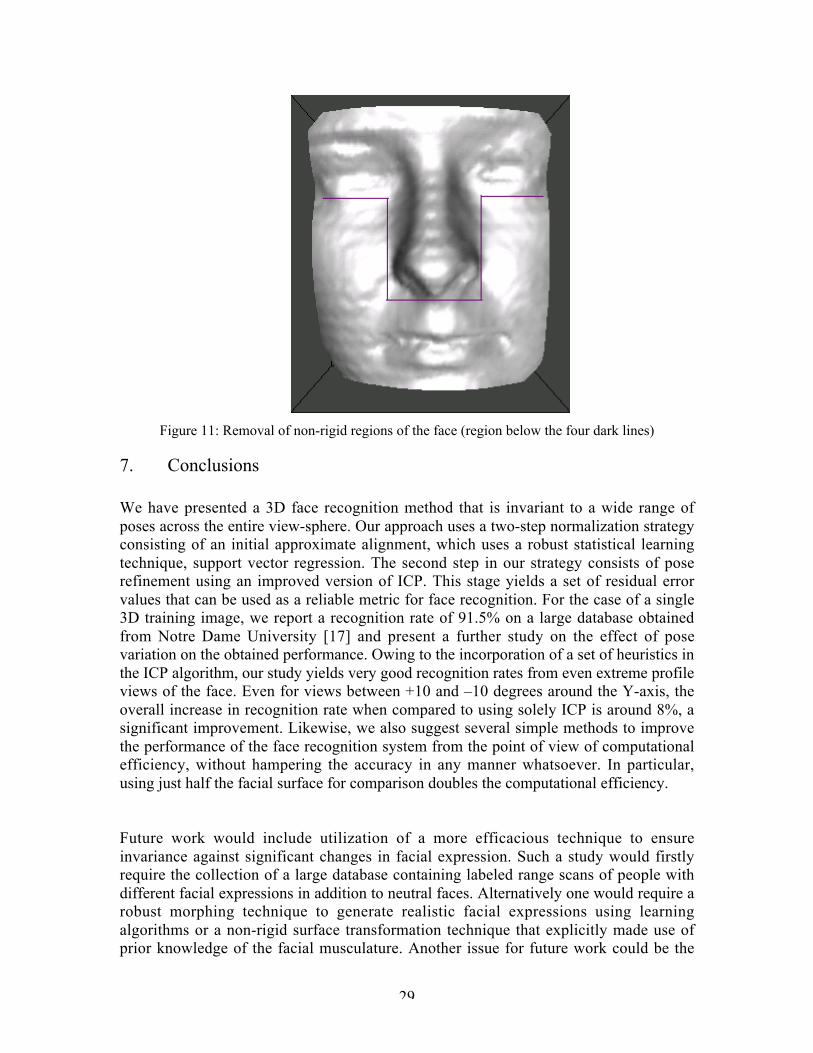
In order to fully automate the process of discarding non-rigid regions, we employ a facialfeature detector to detect the location of the nose, eyes or the mouth (see Figure 11). Wethen apply simple heuristics to identify the deformable regions of the face and finallyperform the usual registration.

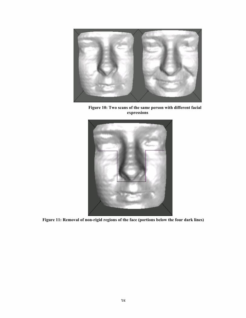
Experiments for testing this technique were performed on the entire Notre Damedatabase. The value of λ was varied from 0 to 1 in steps of 0.1 and the recognition ratewas measured for each value of this parameter. It was observed that the recognition rateactually dropped from 91.5% to around 89.4% if the non-rigid regions were totallydiscarded (i.e., λ was set to 0). This was owing to the fact that some discriminatoryinformation was lost when totally discarding areas such as the cheek and the mouth. Thebest recognition rate (92.3%) was attained when λ was set to a value of 0.3. For allvalues of this parameter less than or equal to 0.5, it was observed that different scans ofone and the same individual carrying significantly different facial expressions were

27

always registered to lower residual error values than before the employment of thisheuristic. Figure 10 shows a pair of scans of the same person with discernibly differentfacial expressions. Figure 11 shows the lines of demarcation between the rigid and non-rigid regions of the face.

We note that the value of λ is likely to be dependent on the specific database used for theexperiments. Ideally, we could have learnt the weights on a validation set consisting ofscans of individuals, each with several different facial expressions (such as frown, smile,or laugh). A second approach would be to apply a part-based technique such as non-negative matrix factorization (NMF) [46] for the purpose of facial recognition (after posenormalization). Using NMF, one could expressly quantify which specific regions of theface contain greater discriminatory power under variation in facial expression. However,the lack of any such existing facial database was the major impediment in performingthese experiments. The Notre Dame database has very few individuals with imagesdisplaying significantly different facial expressions.

Figure 8: Recognition rate versus image size

28

Figure 9: Recognition rate versus number of training images

Figure 10: Two scans of the same person with different facialexpressions

29

Figure 11: Removal of non-rigid regions of the face (region below the four dark lines)

7. Conclusions

We have presented a 3D face recognition method that is invariant to a wide range ofposes across the entire view-sphere. Our approach uses a two-step normalization strategyconsisting of an initial approximate alignment, which uses a robust statistical learningtechnique, support vector regression. The second step in our strategy consists of poserefinement using an improved version of ICP. This stage yields a set of residual errorvalues that can be used as a reliable metric for face recognition. For the case of a single3D training image, we report a recognition rate of 91.5% on a large database obtainedfrom Notre Dame University [17] and present a further study on the effect of posevariation on the obtained performance. Owing to the incorporation of a set of heuristics inthe ICP algorithm, our study yields very good recognition rates from even extreme profileviews of the face. Even for views between +10 and –10 degrees around the Y-axis, theoverall increase in recognition rate when compared to using solely ICP is around 8%, asignificant improvement. Likewise, we also suggest several simple methods to improvethe performance of the face recognition system from the point of view of computationalefficiency, without hampering the accuracy in any manner whatsoever. In particular,using just half the facial surface for comparison doubles the computational efficiency.

Future work would include utilization of a more efficacious technique to ensureinvariance against significant changes in facial expression. Such a study would firstlyrequire the collection of a large database containing labeled range scans of people withdifferent facial expressions in addition to neutral faces. Alternatively one would require arobust morphing technique to generate realistic facial expressions using learningalgorithms or a non-rigid surface transformation technique that explicitly made use ofprior knowledge of the facial musculature. Another issue for future work could be the

30

examination of the effects of occlusion (over different parts of the face) and aging on theoverall recognition rates.

It is curious that 3D face recognition rates are in general lower than the 2D resultsobtained to date. It was always thought that because 3D information provided a morerealistic characterization of the face, it would easily outperform 2D video data. Even thecombination of 2D and 3D, although better, has not produced spectacular results. Thus itmust be asked whether the 2D data actually “mask” certain effects such as facialexpressions. Another possibility is the state of the art of 3D techniques, which has beenaddressed by relatively few researchers. This is probably due to the lack of adequate 3Ddatabases. Perhaps more importantly, it should also be noted that when humans look at2D facial images they do not have any problem recognizing their identity. This isdefinitely not the case with 3D facial images. With the impending development of smalland inexpensive 3D sensors, it is clear that serious questions need to be asked about theiruse for non-rigid object recognition.

References

[1] J. Daugman, “Face and Gesture Recognition: Overview”, IEEE Transactions onPattern Analysis and Machine Intelligence, Vol. 19. No. 7, pp. 675-676, 1997.

[2] C. Burges, “A Tutorial on Support Vector Machines for Pattern Recognition”,Data Mining and Knowledge Discovery, Vol. 2, No. 2, pp. 121-167, 1998.

[3] V. Vapnik, “Statistical Learning Theory”, John Wiley and Sons, New York, 1998[4] A. Schmola and A. Scholkopf, “A Tutorial on Support Vector Regression”,

NeuroCOLT2 Technical Report NC2-TR-1998-030, 1998[5] D. Tax and R. Duin, “Support Vector Domain Description”, Pattern Recognition

Letters, Vol. 20, pp. 1191-1199, 1999.[6] K. Bennet and C. Campbell, “Support Vector Machines: Hype or Hallelujah?”

SIGKDD Explorations, Vol. 2, No.2, pp. 1-13, 2000.[7] S. Li, Q. Fu, L. Gu, B. Scholkopf, Y. Cheng, H. Zhang, “Kernel based Machine

Learning for Multi-View Face Detection and Pose Estimation”, Proceedings ofthe International Conference on Computer Vision, Vol. 2, pp. 674-679, 2001.

[8] P. Besl and N. McKay, “A Method for Registration of 3D Shapes”, IEEETransactions on Pattern Analysis and Machine Intelligence, Vol. 14, No. 2, pp.239-256, 1992.

[9] M. Turk and A. Pentland, “Eigenfaces for Recognition”, Journal of CognitiveNeuroscience, Vol. 3, pp. 71-86, 1994.

[10] C. Hesher, A. Srivastava and G. Erlebacher, “Principal Component Analysis ofRange Images for Facial Recognition”, Proceedings of CISST, Las Vegas, June2002.

[11] F. Tsalakanidou, D. Tzovaras and M. Strintzis, “Use of Depth and ColorEigenfaces for Face Recognition”, Pattern Recognition Letters, Vol. 24, pp. 427-1435, 2003.

31

[12] B. Achermann, X. Jiang and H. Bunke, “Face Recognition using Range Images”,Proceedings of the International Conference on Virtual Systems and Multimedia,pp. 129-136, 1997.

[13] P. Jonathan Phillips, H. Moon, S. Rizvi and P. Rauss, “The FERET EvaluationMethodology for Face-Recognition Algorithms”, IEEE Transactions on PatternAnalysis and Machine Intelligence, Vol. 22, No. 10, pp. 1090-1104, October2000.

[14] H. Tanaka, M. Ikeda and H. Chiaki, “Curvature-Based Face Surface RecognitionUsing Spherical Correlation Principal Directions for Curved Object Recognition”,Proceedings of the Third International Conference on Automated Face andGesture Recognition, pp. 372-377, 1998.

[15] Fisher and Lee, “Correlation Coefficients for Random Variables on a Unit Sphereor Hypersphere”, Biometrica, No. 73, pp. 159-164, 1986.

[16] G. Gordon, “Face Recognition Based on Depth Maps and Surface Curvature”,Geometric Methods in Computer Vision: SPIE, pp. 1-12, 1991.

[17] K. Chang, K. Bowyer and P. Flynn, “Face Recognition Using 2D and 3D FacialData”, 2003 Multimodal User Authentication Workshop, pp. 25-32, December2003.

[18] A. Moreno, A. Sanchez, J. Velez and F. Diaz, “Face Recognition using 3DSurface-extracted Descriptors”, Proceedings of Irish Machine Vision and ImageProcessing Conference, September 2003.

[19] R. Duda and P. Hart, “Pattern Classification and Scene Analysis”, New York:Wiley and Sons, 1973.

[20] J. Lee and E. Milios, “Matching Range Images for Human Faces”, Proceedings ofthe International Conference on Computer Vision, pp. 722-726, 1990.

[21] C. Chua and R. Jarvis. “Point Signatures: A New Representation For 3D ObjectRecognition”, International Journal Computer Vision, Vol. 25, No. 1, pp. 63-85,1997.

[22] C. Chua, F. Han, Y. Ho, “3D Human Face Recognition Using Point Signature”,Proceedings of the Fourth IEEE International Conference on Automatic Face andGesture Recognition, pp. 233-239, 2000.

[23] Y. Wang, C. Chua and Y. Ho, “Facial Feature Detection and Face Recognitionfrom 2D and 3D Images”, Pattern Recognition Letters, Vol. 23, pp. 1191-1202,2002.

[24] Y. Chen and G. Medioni, “Object Modeling by Registration of Multiple RangeImages”, Proceedings of the International Conference on Robotics andAutomation, 1991.

[25] X. Lu, D. Colbry and A. Jain, “Three Dimensional Model-Based FaceRecognition”, Proceedings of the International Conference on PatternRecognition, 2004.

[26] X. Lu, D. Colbry and A. Jain, “Matching 2.5D Scans for Face Recognition”,Proceedings of the International Conference on Biometric Authentication (ICBA),2004.

[27] P. Phillips, P. Grother, R. Michaels, D. Blackburn, E. Tabassi and J. Bone,“FRVT 2002: A Overview and Summary”, March 2003.

32

[28] Y. Li, S. Gong, H. Liddell, “Support Vector Regression and Classification BasedMulti-View Face Detection and Recognition”, Proceedings of the IEEEInternational Conference on Automatic Face and Gesture Recognition, pp. 300-305, 2000.

[29] M. Motwani and Q. Ji, “3D Face Pose Discrimination Using Wavelets”,Proceedings of the International Conference on Image Processing, Vol. 1, 1050-1053, 2001.

[30] J. Sherrah, S. Gong and E. Ong, “Face Distributions in Similarity Space UnderVarying Head Pose”, Image and Vision Computing, Vol. 19, pp. 807-819, 2001.

[31] A. Rajwade and M. Levine, “Facial Pose from 3D Data”,http://www.cim.mcgill.ca/~levine/FacialPose_from_3d_Data.pdf, Submitted

[32] V. Blanz and T. Vetter, “A Morphable Model for the Synthesis of 3D Faces”,Proceedings of SIGGRAPH, pp. 353-360, July 1999.

[33] N. Amenta, S. Choi and R. Kolluri, “The Power Crust”, Sixth ACM Symposium onSolid Modeling and Applications, pp. 249-260, 2001.

[34] C. Chang and C. Lin, “LIBSVM: a Library for Support Vector Machines”,http://www.csie.ntu.edu.tw/~cjlin/libsvm/, 2001.

[35] F. A. Sadjadi and E. L Hall, “Three-dimensional Moment Invariants”, IEEETransactions on Pattern Analysis and Machine Intelligence, Vol. 2, No. 2, pp.127-136, March 1980.

[36] J. Feldmar and N. Ayache, “Rigid, Affine and Locally Affine Registration ofFree-form Surfaces”, International Journal of Computer Vision, Vol. 18, No.2,pp. 99-119, 1996.

[37] Z. Zhang, “On Local Matching of Free-form Curves”, Proceedings of the BritishMachine Vision Conference, pp.347-356, 1992

[38] T. Masuda, K. Sakaue and N. Yokoya, “Registration and Integration of MultipleRange Images for 3D Model Construction”, Proceedings of the InternationalConference on Computer Vision and Pattern Recognition, pp. 879-883, 1996.

[39] F. Preparata and M. Shamos, “Computational Geometry”, Springer Verlag, 1985.[40] J. Bentley, “K-d Trees for Semidynamic Point Sets”, Proceedings of the 6th

Annual Symposium on Computational Geometry, pp. 187-197, 1990.[41] http://ph.konicaminolta.com.hk/eng/industrial/3d.htm, “Minolta Vivid Range

Scanner”.[42] A. Fitzgibbon, “Robust Registration of 2D and 3D Point Sets”, Proceedings of the

British Machine Vision Conference, pp. 411-420, 2001.[43] W. Press, S.Teukolsky, W. Fetterling and B. Flannery, “Numerical Recipes in C:

The Art of Scientific Computing”, Cambridge University Press, Cambridge,1992.

[44] H. Chui and A. Rangarajan, “A New Algorithm for Non-rigid Point Matching”,IEEE Conference on Computer Vision and Pattern Recognition, Vol. 2, pp. 44-51,2000.

[45] T. Jost and H. Hugli, “A Multi-Resolution Scheme ICP Algorithm for Fast ShapeRegistration”, Proceedings of the First International Symposium on 3D DataProcessing Visualization and Transmission, pp. 540-543, Padova, Italy, June2002.

33

[46] D. Lee and H. Seung, “Learning the Parts of Objects by Non-Negative MatrixFactorization”, Nature, Vol. 401, pp. 788-791, 1999.

34

FIGURES

Figure 1: Sample Faces from the Freiburg Database

Figure 2: Faces from the Notre Dame Database

Figure 3: A Few Cropped Models from the Notre Dame database

35

Figure 4: Corresponding Cropped probe images from the Notre Dame database

Figure 5: Residual Error Values between different images of the same persons

36

Figure 6:Residual Error Values between different images of different persons

Figure 7: Residual Error Histogram for images of the SAME (red) and DIFFERENT(green) people shown together for comparison

37

Figure 8: Recognition Rate versus Image Size

Figure 9: Recognition Rate versus Number of Training Images

38

Figure 10: Two scans of the same person with different facialexpressions

Figure 11: Removal of non-rigid regions of the face (portions below the four dark lines)

39

TABLES

Results for Y-angle (Freiburg

Database)

Results for X-angle (Freiburg

database)

Results for Y-angle (Notre

Dame Database)

Results for X-angle (Notre

Dame database)Number of supportvectors (percentageof training samples)

12% 14% 12% 14%

Frequency of errorless than +/- 3

degrees

70.09% 73.23% 66% 69.23%

Frequency of errorless than +/- 6

degrees

94.92% 95.97% 91.92% 92%

Frequency of errorless than +/- 9

degrees

98.85% 99.23% 96.86% 98.61%

Average PoseEstimation error(Absolute Value)

2.8 degrees 2.58 degrees 3.2 degrees 2.72 degrees

Table 1:Results of Pose Estimation

Face Recognition Rates (Percentage)Angle of rotation of probes(Around Y-axis) ICP ICP Variant

(this paper)LMICP

+/- 10 degrees 83.8 91.5 84.2+/- 20 degrees 80.5 90 80.5+/- 30 degrees 78.5 86.6 78.4+/- 40 degrees 76.3 84 76.4+/- 50 degrees 73.5 81.5 74.5

Table 2:Recognition Rates with ICP, ICP Variant and LMICP

Face Recognition Rates(Percentage)

Angle of rotation of probes(Around Y-axis)

Features +ICP

Features +ICP Variant

+/- 10 degrees 83.8 91.5+/- 20 degrees 82.5 90.5+/- 30 degrees 81.5 88.3+/- 40 degrees 78.5 86+/- 50 degrees 77 84.5

Table 3:Recognition Rates with ICP and the ICP Variants after applying the feature-basedmethod as an initial step

40

Face Recognition Rates (Percentage)Angle of rotation of probes(Around Y-axis) SVR + ICP SVR + ICP Variant+/- 10 degrees 83.0 91.5

Angles between +/- 20 to +/- 50 degrees 81.16 88Angles between +/- 50 to +/- 90 degrees 80.5 87

Table 4:Recognition rates with ICP and ICP variant after applying SVR as the initial step