20060516058 4-18 pscad current source comparison ..... 41 figure 5-1 b aseline ips ..... 45 figure...
TRANSCRIPT

DISTRIBUTION STATEMENT AApproved for Public Release
Distribution Unlimited
Analysis of Harmonic Distortion in an Integrated Power System for Naval Applicationsby
Edward G. WestB.S.E., Electrical Engineering
The Citadel, 1999
Submitted to the Department of Ocean Engineering and the Department of ElectricalEngineering and Computer Science in Partial Fulfillment of the Requirements for the Degrees of
Naval Engineer
and
Master of Science in Electrical Engineering and Computer Science
at theMassachusetts Institute of Technology
June 2005© 2005 Edward G. West. All rights reserved.
The author hereby grants to MIT and the United States Government permission to reproduce andto distribute publicly paper and electroni popie f this tesis document in whole or in part.
Signature of Author .-.... _ -Department of Ocean Engineering and the
t of Electrical Engineering and Computer ScienceCMay 12, 2005
Certified by
Timothy J. MýCo -, Assciate Professor of Nava-tonstruction and EngineeringDepartment of Ocean Engineering
/ ,ii fThesis SupervisorCertified by
aes Kirtley, Professor of Electrical Engineering and Computer ScienceDepart ent of Electrical Engineering and Computer Science
Thesis Reader
Accepted by
A ,iael Triantafyllou, Professor of Ocean Engineering.. iCharn, Department Comittee on Graduate Students
Accepted .•by. / 7J" ._"par rei Q. ean EngineeringAccepted by _ -. " . . --.... • r _..
Aftihur C. Smith, Professor of 1gctrica Engineering and Computer ScienceChairman, Department Committee on Graduate Students
Department of Electrical Engineering and Computer Science
20060516058

Page Intentionally Left Blank
2
Analysis of Harmonic Distortion in an Integrated Power System for Naval Applicationsby
Edward G. West
Submitted to the Department of Ocean Engineering and the Department of ElectricalEngineering and Computer Science in Partial Fulfillment of the Requirements for the Degrees of
Naval Engineer
and
Master of Science in Electrical Engineering and Computer Science
ABSTRACT
This research quantifies the voltage distortion over the broad range of operating conditionsexperienced by a Naval warship. A steady state model of an Integrated Power System (IPS) wasdeveloped in a commercially available power system simulation tool. The system chosen for thisstudy was a three-phase, 4160 VAC, 80 MW power system with a 450 VAC bus to supplytraditional ship service loads. Sensitive loads, such as combat systems equipment, are isolatedfrom the harmonic content of the 450 volt bus via solid state inverters. Power generation for thissystem included two 30 MW and two 10 MW generators. The sizing of these generators wasbased on operating configurations that would result in the best fuel efficiency under the mostcommon loading conditions. Model components were simulated and compared to data recordedfor the U.S. Navy's Full Scale Advanced Development (FSAD) test system for the IPS at thePhiladelphia Land Based Engineering Site (LBES). The propulsion motor used in thesimulations was developed based on the advanced induction motor installed at LBES. Variousloading conditions, including battle, cruise and anchor were simulated for both 10°F and 90'Fambient design conditions and with propulsion loads ranging from 0% to 100%. Numeroussystem configuration changes were implemented to determine their impact on system harmonics.These included operating the propulsion converter front end rectifiers in both controlled (varyingcommutation angle) and uncontrolled (diode bridge) configurations; implementation of bothtwelve and six pulse rectification; and installation of a tuned passive 5th harmonic filter. Thesimulation results are compared to both IEEE Std 519-1992 and Mil-Std 1399.
Thesis Supervisor: Timothy McCoyTitle: Associate Professor of Ocean Engineering
Thesis Reader: James KirtleyTitle: Professor of Electrical Engineering and Computer Science
3

Page Intentionally Left Blank
4

Table of Contents
Table of Contents ............................................................................................................................ 5List of Figures ................................................................................................................................. 7List of Tables .................................................................................................................................. 9Chapter 1 Introduction ............................................................................................................... 11
1.1 Purpose .......................................................................................................................... 111.2 Problem ......................................................................................................................... 111.3 Scope ............................................................................................................................. 13
Chapter 2 M easures of Distortion ........................................................................................... 15Chapter 3 H arm onic Analysis ................................................................................................ 21
3.1 Frequency Dom ain .................................................................................................... 213.1.1 Frequency Scan .................................................................................................. 213.1.2 Current Source Injection .................................................................................. 223.1.3 H arm onic Load Flow ........................................................................................ 23
3.2 Tim e Dom ain ................................................................................................................ 24Chapter 4 M odel Validation .................................................................................................. 27
4.1 Test System Com parison ........................................................................................... 274.2 LBES System Com parison ...................................................................................... 30
4.2.1 Generator ............................................................................................................... 304.2.2 H arm onic Filter .................................................................................................. 324.2.3 Induction M otor ............................................................................................... 334.2.4 Sim ulation Results ........................................................................................... 35
4.3 Harm onic Source Com parison .................................................................................. 394.4 M odel Validation Sum m ary ....................................................................................... 41
Chapter 5 Integrated Power System Developm ent ................................................................ 435.1 Approach and Assum ptions ...................................................................................... 435.2 System Description .................................................................................................. 43
5.2.1 Generator ............................................................................................................... 465.2.2 450 V Distribution and CAPS/A GS ................................................................. 515.2.3 Six Pulse Induction M otor Drive ...................................................................... 52
Chapter 6 Baseline Sim ulations and M itigation Techniques ................................................ 536.1.1 THD on the 450 V bus ...................................................................................... 566.1.2 Generator Current Distortion ........................................................................... 626.1.3 Baseline Sim ulation Conclusions .................................................................... 63
6.2 H arm onic Distortion M itigation Techniques .......................................................... 656.2.1 Line Com m utated Rectifier M otor Drive ........................................................ 656.2.2 Multipulse Motor Drive and Harmonic Filter Systems .................................... 69
6.3 Overall Conclusions .................................................................................................. 75Chapter 7 Subtransient Reactance ........................................................................................ 77
7.1 Fault Current ................................................................................................................. 777.2 V oltage Distortion ........................................................ ................................................. 797.3 Impact on the Baseline System ................................................................................ 82
Chapter 8 Conclusions ............................................................................................................... 85
5

8.1 Future W ork .................................................................................................................. 87List of References ......................................................................................................................... 89Appendix A . M atlab Scripts ............................................................................................... 93Appendix B. LBES Comparison for Generator, Filter, and Voltage ................................. 99Appendix C. Tabulated Distortion Results ........................................................................... 107
6

List of Figures
Figure 2-1 Full Bridge Rectifier ............................................................................................... 15Figure 2-2 Full Bridge Voltage and Current ............................................................................. 15Figure 2-3 Bridge Rectifier with Output Filter ......................................................................... 16Figure 2-4 Current D istortion .................................................................................................... 19Figure 3-1 Six Pulse Rectifier alpha = 0 degrees ....................................................................... 22Figure 3-2 Six Pulse Rectifier alpha = 45 degrees .................................................................... 23Figure 3-3 Up/Down Converter ............................................................................................... 25Figure 4-1 T est System ................................................................................................................. 28Figure 4-2 PSCAD/EMTDC Simulation ................................................................................. 29Figure 4-3 A CSL Sim ulation .................................................................................................... 29Figure 4-4 SABRE Simulation ....... ...................................... 29Figure 4-5 LBES Components .................................................................................................. 30Figure 4-6 Simplified Model Motor and Generator Current ................................................... 31Figure 4-7 Detailed Model Steady State Generator and Motor Current .................................. 31Figure 4-8 Firing Angle vs Speed .......... ................................. 34Figure 4-9 Induction Motor Drive Circuit .................................................................................... 34Figure 4-10 LBES 90% Harmonic Magnitude Comparison .................................................... 36Figure 4-11 LBES 90% Power Motor Current ........................................................................ 36Figure 4-12 LBES 50% Harmonic Magnitude Comparison ................................................... 37Figure 4-13 LBES 50% Motor Current ................................................................................... 37Figure 4-14 LBES 10% Harmonic Magnitude Comparison .................................................... 38Figure 4-15 LBES 10% Motor Current ................................................................................... 38Figure 4-16 Current Source Comparison Circuit ...................................................................... 39Figure 4-17 Phase-to-Neutral Equivalent Circuit .................................................................... 41Figure 4-18 PSCAD Current Source Comparison .................................................................... 41Figure 5-1 B aseline IPS ................................................................................................................ 45Figure 5-2 Synchronous Machine Transient Model ................................................................. 48Figure 5-3 Steady State Synchronous Machine Model ............................................................. 49Figure 5-4 Future Surface Combatant Power Requirements ......................... 51Figure 6-1 Voltage and Current 10% Power .............................................................................. 56Figure 6-2 Voltage and Current 90% Power .............................................................................. 56Figure 6-3 THD 450 V Baseline System ................................................................................. 58Figure 6-4 THD vs Speed, Cruise Loading, 90 degree day ...................................................... 59Figure 6-5 Individual Harmonic Voltages, Cruise Loading, 90 degrees ................................. 60Figure 6-6 Individual Harmonic Voltages, Cruise Loading, 10 Degrees ................................. 60Figure 6-7 Individual Harmonic Voltages, Battle Loading, 10 degrees ................................... 61Figure 6-8 Individual Harmonic Voltages, Battle Loading, 10 degrees ................................... 61Figure 6-9 Harmonic Current Magnitude (RMS) 10 MW Generator ...................................... 62Figure 6-10 Harmonic Current Magnitude (RMS) 30 MW Generator .................................... 63Figure 6-11 Generator Current, 10 deg day, 25 knots ............................................................. 64Figure 6-12 Generator Current, 10 deg day, 25 knots, 5th and 7th Harmonics Removed ..... 64
7
Figure 6-13 Propulsion M otor Firing Angle ............................................................................. 66Figure 6-14 Six Pulse Line Commutated Propulsion Converter ............................................ 67Figure 6-15 THD Comparison, Line Commutated vs Phase Controlled Motor Drive ............. 67Figure 6-16 Individual Harmonic Current (10 M W Generator) ............................................... 68Figure 6-17 Individual Harmonic Current (30 M W Generator) ............................................... 68Figure 6-18 12 Pulse Converter ............................................................................................... 70Figure 6-19 12 Pulse Line Current ........................................................................................... 71Figure 6-20 THD Comparison ................................................................................................. 72Figure 6-21 Filter System THD ............................................................................................... 72Figure 6-22 THD 12 Pulse System ................................................................................. * ............. 73Figure 6-23 Individual Distortion 12 Pulse System .................................................................. 74Figure 6-24 Individual Distortion, Filter System .......................................................................... 74Figure 6-25 Summary of Distortion Results ............................................................................. 75Figure 7-1 Generator Fault Current .......................................................................................... 78Figure 7-2 Generator Fault Current vs. Installed Power ........................................................... 79Figure 7-3 Subtransient Reactance Simulation Circuit ............................................................. 80Figure 7-4 Voltage Distortion .................................................................................................... 81Figure 7-5 Current Distortion ................................................................................................... 81Figure 7-6 Voltage Distortion vs M otor Drive Power .................................................................. 82Figure 7-7 THD% with 22% Subtransient Reactance ............................................................... 83
8

List of Tables
Table 4-1 Parameter Values for Test System .......................................................................... 28Table 4-2 Generator Parameters ............................................................................................... 32Table 4-3 Harmonic Filter Parameters ...................................................................................... 32Table 4-4 Motor Drive Parameters .......................................................................................... 33Table 4-5 Tabulated LBES Simulation Results ........................................................................ 39Table 5-1 Future Surface Combatant Ship Service Power Requirements ............................... 52Table 6-1 IEEE STD 519 Harmonic Current Profile ............................................................... 54Table 6-2 Generator Current Ratings ......................................................................................... 55Table 6-3 Size and Weight of Harmonic Filter and Propulsion Transformers ........................ 76Table 8-1 Turbine/Generator Sets ............................................................................................. 86Table 8-2 Cruise Loading, 90 Degrees, Baseline System ........................................................... 107Table 8-3 Cruise Loading, 10 Degree, Baseline System ............................................................ 108Table 8-4 Battle Loading, 90 Degree, Baseline System ............................................................. 109Table 8-5 Battle Loading, 10 Degrees, Baseline System ............................................................ 110Table 8-6 Anchor Loading, Baseline System ............................................................................. 111Table 8-7 Line Commutated System, 90 Degree Day, Cruise Loading ..................................... 112Table 8-8 Filter System Tabulated Results ................................................................................. 113Table 8-9 12 Pulse System Tabulated Results ............................................................................ 114
9

This page intentionally left blank.
10

Chapter 1 Introduction
1.1 Purpose
The purpose of this thesis is to develop accurate models of power electronic devices that
will be installed on future naval warships. These models will be used to analyze the harmonic
distortion on the main electrical busses under a variety of operating conditions. The impact of
harmonic mitigation techniques on an Integrated Propulsion System will also be analyzed.
1.2 Problem
The Navy envisions a significantly greater role of electrically powered systems in future
naval warships. This is represented by the commitment to an Integrated Power System (IPS) for
the next generation warship.[1] A ship configured with IPS uses an electrical motor to drive the
speed of the propeller, eliminating the need for a reduction gear and long shaft. A common
electrical bus provides the ships electrical power and propulsion power. A traditional non-IPS
surface combatant dedicates over two thirds of its power generation capability to turning its
propellers. This generation capacity is not available for anything other than propulsion and is
typically represented by four prime movers. Additional prime movers are required for
generation of electricity for ship loads. Some of the advantages of an IPS arrangement are listed
below.[2]
"* Increased fuel economy due to the efficient operation of prime mover
"* Arrangement flexibility due to the elimination of large mechanical shaft
components and the reduction of total prime movers
"* Availability of a large amount of electrical power for non-propulsion use
"* Ability to accommodate the electrical power needs of future military systems
"* Reduced manning requirements due to high levels of automation and control
The successful implementation of IPS is only possible due to advances in high voltage,
high power semiconductor switching devices. These advances in power electronics have made
propulsion systems utilizing variable speed AC motor drives cost competitive with traditional
mechanical drive plants. [ 1] [2] Additionally, weapons systems and high power radars are
expected to have a similar power electronic interface with the main bus distribution systems.
11

The installation of these power electronic devices will have a negative impact on main
bus power quality. The deleterious effect is due to the fact that these loads do not draw purely
sinusoidal current. The non linear circuit elements in these circuits distort the current waveform
and result in harmonics of the fundamental frequency. In this paper the terms non-linear and
harmonic will be used when describing loads exhibiting these characteristics. The power supply
for these loads usually requires use of a bridge rectifier at the front end. The bridge rectifier
draws current at harmonics of the fundamental frequency from the distribution system. When
these currents propagate through the distribution system they develop voltage across the
impedance of the source. This leads to distortion of the voltage waveform seen by all loads in
the distribution system. Distortion of supply voltage can lead to improper operation of sensitive
electronic equipment and overheating of certain elements in the power system such as motors,
transformers, and cables.
Interest in power system harmonics dates to the early 1930's when utilities first noticed
distorted voltage and current waveforms on overhead transmission lines. At the time, their
interest was primarily in the effect on electric machines, telephone interference, and power
capacitor failure. [6] Over the last twenty years the proliferation of electronic switching into
power electronics devices has caused renewed interest in power system harmonic studies.
Concerns over the increase in non-linear loads have shown the need for harmonic studies as a
standard component of power system analysis and design. [7]
A navy ship with IPS can be regarded as a small scale, autonomous, industrial type power
system sharing the same power quality concerns as the utilities. The modern warship, like the
continental grid, has experienced the same proliferation of power electronics and shares the need
for analysis of power system harmonics. However, there are several differences between a land
based distribution system and ship based system. [8] They are:
"* The ships power system is completely autonomous. Reliability is essential for
safety of the ship and crew
"* The relative rotational inertia of the prime movers is small compared to the
electrical load
"* The ships distribution system consists of AC and DC voltage at different
magnitudes and frequencies
"* The ships grid has cables of short length compared to land based systems
12

A significant portion of the total ships load draws non-linear current
These differences make the accurate representation of harmonic generating devices within the
IPS imperative for the design and analysis of this system.
1.3 Scope
This research will be accomplished in three steps. The fist step will involve developing
accurate models of non-linear power system components for an IPS. In the second step, a
notional distribution system with loads representative of a future surface combatant will be
developed. The final step will be to analyze this notional IPS for voltage and current distortion
over the wide range of operating conditions experienced by Navy ships at sea.
13

This page intentionally left blank.
14

Chapter 2 Measures of Distortion
The simple full bridge rectifier shown in Figure 2-1 and its associated voltage and current
waveforms, Figure 2-2 and Figure 2-3 , will be used to illustrate some characteristics of power
system harmonics.
Figure 2-1 Full Bridge Rectifier
"Idc
• +
Vdc
Figure 2-2 Full Bridge Voltage and Current
112 W2160 .DO
100.00----------------------- -- --------- -- - - -
120.00
60.00..... ..... ..... ..... .......... ....--.------ . ---- -- -- ---- ---- -- ---- --
100,00 -0-0-00 10 10-0.00 0 1-00.00
.150.00 ................ ... -: ... . .. . . . . ... .. .. ............. ............................... .... ............ ............ ........III "VP1
120.013
0 .Da - -- ----
"Time (ms)
15

Figure 2-3 Bridge Rectifier with Output Filter
112 W2160.00
100.00 - - - - - - - -- - - - - - - - - - -- - - - - - -j- - - - - - - -
-100.00 ----.--...... . .. -...-....- -.................. ........ .........15n 00 ..... .I . .. .V . . ........... . . ..... ...................... .. .. ..............
Ml \/i120.00
100.00- -- -- - - - --- - --- - - - -- - - - -- - - -
I0.0 --V---------------- ---------------- --------------------------
0.0o0o --------e------------ ------ -.----- -... .... ..... ---e .oD I . . . . . . .-- -- - ... .. .d ... .. .. . . . . . . ... ..... ..... ................. .............. ........ .. . . . . .
1010.00 1020.013 1030.020 1040.038 1060.061 1000.004Time (ms)
Figure 2-2 shows the voltage and current waveforms of the bridge rectifier with the
output capacitor set at 0, and assuming ideal diodes. The source current is transferred between
the diodes the moment the source voltage changes polarity. In a real bridge rectifier, the source
will have some amount of inductance and typically an output capacitor will be installed to reduce
the ripple of the output voltage. Figure 2-3 shows the same bridge rectifier waveforms but now
with an output capacitor. The output capacitor prevents the diodes from turning on until the
polarity of the source voltage is greater than the voltage on the output capacitor. This results in
regularly appearing distortion of the source current at a multiple of the source frequency as
evidenced by the source current waveform of Figure 2-3. This distortion is referred to as
harmonic distortion.
In order to measure harmonic distortion Fourier analysis is used. Fourier analysis allows
us to represent any periodic wave form as a Fourier series. [9][10] [16] Consider a periodic
functionf(t). This function can be represented as:
f(t) = CO + , Cn cos(nx + Oj)n=l
Equation 2-1
16

Cn = • + Bn On =tan-'(-B./A,,)
With T=21rco the coefficients An, Bn, and Co are defined as: (note: T must be a multiple of a
period)
An =- f(t)cos(nci)dt Bn = T-f (t)sin(nao)dt CO= f (t)dt
Equation 2-2
Using Equation 2-1 and Equation 2-2 we will determine a measure of the distortion of the
line current in Figure 2-2. Assume that the voltage input is purely sinusoidal and is given by:v5 -2Vi sin colt
Equation 2-3
The input current into the bridge rectifier can be written as a sum of its Fourier components.
i, (t) = i sl (t) + I i ,h Wt
h#1
i'l= i]2IIl sin(o 1t - 01) and ih = 4Iih sin(coht - Oh
Equation 2-4
The rms value of i, (t) is:
I, *Ji,(t)dt
Equation 2-5
Substituting Equation 2-4 gives:
I,= 1s2 1+ 2h
Equation 2-6
17

Define the distortion current, (idis(t)), as that component of the current not at the fundamental
frequency then this current (rms) is given by:
SII =i-/
7~1
Equation 2-7
%THD can now be defined as:
%THD= =100* =100*- =100"
Is1 Ish 1,I
Equation 2-8
Another useful measure of distortion is power factor (PF). [9] [10] Consider the voltage
and current waveforms shown in Figure 2-4. The voltage is purely sinusoidal while the current
is a distorted waveform containing the first and fifth harmonic.
18

Figure 2-4 Current Distortion
3
Voltage
2- -- Current
1 Fundemr n al Cent
-1
"2-
-310 0.005 0.01 0.015 0.02 0.025 0.03 0.035
The average power can be calculated by:
P = p(t)dt = f- vs (t)i, (t)dt
Equation 2-9
Substituting Equation 2-3 and Equation 2-4:
P= 1J f-vV sin Oat *JIsi, sin(O)lt- 1)dt=VsIs cosobiTo
Equation 2-10
Note that the only component of the current that contributes to the average power drawn from the
source is the fundamental current. For sinusoidal quantities the apparent power (S) and the
power factor (PF) are defined as:
S =VSIS
19

Equation 2-11
PPF=-
S
Equation 2-12
Using Equation 2-10 and Equation 2-11:
PF = Vl,,cos A =,Cs_ cVsI, Is
Equation 2-13
Equation 2-13 shows that when dealing with distorted waveforms there are two components that
effect PF, the displacement factor, k, = cos 0, and the distortion factor, kd = I"a kd. ko is theIs
familiar power factor angle and represents the phase difference between the voltage and current.
kd is a measure of the amount of distortion in the line current of a load. When both the current
and voltage are sinusoidal kd = 1. It is sometimes useful to represent PF using THD.
1 1PF kdk - isko ko
1+ THD 2
Equation 2-14
20

Chapter 3 Harmonic Analysis
Harmonic analysis of power systems can be conducted in both the frequency domain and the
time domain. An overview of the various techniques will be presented.
3.1 Frequency Domain
Frequency domain analysis requires development of the admittance matrix of the system.
This method is based on multi-port network theory. The positive sequence admittance matrix is
developed from component level two port admittance parameters. A detailed discussion of this
method can be found in [6] and [16]. The admittance matrix must be determined for each
frequency of interest. Various frequency domain algorithms are used in conjunction with the
admittance matrix in order to conduct the analysis.
3.1.1 Frequency Scan
The most common and also the simplest method of analysis is called a frequency scan. This
method involves the solution of Equation 3-1:
ly 1-I= [I.]
Equation 3-1
Where [Y, ] is the admittance matrix, L,'] is the known current vector, and LV] is the nodal
voltage. The subscript n denotes the integer multiple of the base frequency. The system
response as a function of frequency is determined through solution of Equation 3-1 at integer
multiples of the base frequency. If a one per unit sinusoidal current is injected into the system at
a specific point, the corresponding node voltages will represent the driving point impedance of
the system as seen from this point. The frequency is varied from the base frequency to the
highest harmonic frequency of interest and then the impedance over this range can be plotted.
The peaks of this plot correspond to parallel resonance conditions (high impedance to current
flow), and the valleys of the plot correspond to series resonance conditions (low impedance to
current flow). This method provides an excellent visual indication of resonance conditions and
21

is especially useful when trying to assess the impact of the addition of a new piece of equipment
which draws non-linear current. [6] [16]
3.1.2 Current Source Injection
This method requires information about the magnitude of the current drawn by a non-linear
load in addition to the admittance matrix of the network the load is connected to. Many
harmonic sources can by characterized by a typical spectrum. These spectrums can be found in
references such as [6],[9], and [20]. Equation 3-1 is solved at specific harmonic frequencies and
the voltage at that frequency is obtained. The magnitude of the voltages at each harmonic
frequency can be used in Equation 2-8 to determine THD.
There are some limitations when using this method for calculation of system distortion.
When more than one non-linear load is present this method loses accuracy because it does not
accurately reflect the phase angle of each harmonic. Studies have shown that when more than
one non-linear load is present a significant amount of cancellation, due to difference in phase
angle, takes place. [7] [15] This method is also limited in that many non-linear loads present vary
different harmonic spectra depending on load level or control strategies. Figure 3-1 and Figure
3-2 show the input current to a six pulse rectifier operating at two different thyristor firing
angles. Clearly the harmonic content of these two signals is different.
Figure 3-1 Six Pulse Rectifier alpha =0 degrees
Nbin: Graphs2.0 <A phase2.00-
1.50-
1.00-
0.50-
0.00
-0.50
-1.00-
-1.50-
-2.00
0.3000 0.3050 0.3ioo 0.3150 0.3k0 0.350 0.330 0.3350
22

Figure 3-2 Six Pulse Rectifier alpha =45 degrees
MWin: Gra~hs
2.00
1.50-
1.00-
0.50.0.00-
-0.50-
-1.00-
-1.50-
-2.00J
0.3000 0.3050 0.3100 0.3150 0.£00 0.350 0.330o 0.335
3.1.3 Harmonic Load Flow
This method requires that non-linear load current be represented as a function of harmonic
voltages existing at the device terminals and control variables applicable to the load (ie thyristor
firing angle in a rectifier). In this method variations as depicted in Figure 3-1 and Figure 3-2 can
be accommodated. Each load is represented as follows:
Where Ca, Cb,... represent control variables for load parameters
VI, V2 .... Vn represent harmonic voltages at the device terminals
I. = F(Va,V 2,...V., Ca, Cb ......
Equation 3-2
This representation is used in conjunction with Equation 3-1 to form a complete mathematical
model of the system. These equations are then solved iteratively using Newton or Gaussian
algorithms. The limitation of this technique is that in many cases a representation of the non-
linear loads in the form of Equation 3-2 is not possible. When this is the case, techniques that
represent non-linear loads by their time domain differential equations have been
developed. [6] [16] [20]
23

3.2 Time Domain
Harmonic studies involving widely varied load patterns are often best suited to simulating a
complete time domain model using electromagnetic transient programs such as EMTP or
EMTDC. These programs are based on the principles outlined in [11]. EMTDC
(Electromagnetic Transients including DC) was originally developed as a simulation tool for the
Nelson River HVDC Power System in Manitoba, Canada. EMTDC represents and solves
differential equations in the time domain given a fixed time step. This allows the response of the
system to be solved at all frequencies, limited only by the user selected time step.[ 12] The
method primarily used in this research will be using EMTDC with the graphical interface of
PSCAD.
The network impedance can be represented by models of the components primarily
responsible for the impedance properties of the system. For example, in rotating machines the
magnetic field created by stator time harmonics rotates at speeds significantly higher than the
mechanical speed of the rotor. Therefore, the inductance of a synchronous machine can be
modeled as the negative sequence impedance or the average of the direct and quadrature
subtransient impedances. An induction machine can be approximated as the locked rotor
impedance. Linear passive loads can be modeled as an aggregate load if reasonable estimates of
real power and reactive power are available. [6] [20]
In large networks it may be necessary to represent a portion of the network by its dynamic
equivalent. This strategy represents the driving point and transfer impedances between busses by
a lumped RLC branches. An overview of this technique is outlined in [6].
Harmonic sources can be represented as rigid harmonic sources, as a switching function, or
with detailed models. Rigid harmonic sources are described by Equation 3-3.n
i(t) = I1 cos(wt + 01 ) + In E cos(nwt + On)2
0,, = nO, + (n +1)2"
2
Equation 3-3
The magnitude of the current can be obtained from typical spectrum or from measurements and
the phase angle can be determined from the load power factor.
24

The switching function can be used to determine a state space model for a converter.
Consider the Up/Down converter shown in Figure 3-3:
Figure 3-3 Up/Down Converter
Vin q "L L Rc Vout
C TVc
Let the switching function q(t) = 1 when the transistor is on and q(t) = 0 when the transistor is off
and let q'(t) = 1-q(t). The following equations define the circuit when the q(t)=1.
VL (t) =L diL v, t
dt
c(t)=Cdvc 1 vc(t)dt R+Rc
Equation 3-4
When q(t)=O,
VL(t)=L di R [-RciL(t)+vC(t)I
dt R+Rc
Equation 3-5
Combining Equation 3-4 and Equation 3-5 and introducing q(t) results in the state space model
of the Up/Down converter.[9]
diL • R Rcq'(t)iL(t)+ q'(t)vc (t)]+ 1q(t)Vi(t)
dt L(R +R2 L
25

dvc -1 ,(t)i,(t)+v,(t)]
dt C(R +Rc)
Equation 3-6
The final method is through a detailed representation of the non-linear load and its
associate control mechanisms. Weak systems, such as an IPS, require this method in order to
accurately represent harmonic distortion. The simulation consists of a transient phase followed
by the steady state phase. The transient phase is due to the network natural frequencies and the
interaction between network voltage and frequencies and converter controls. The transient phase
can last as long as ten fundamental cycles. At the end of the transient phase, steady state
conditions should be verified. For example, the average DC current of a converter could be
checked. At steady state this current should be constant. Once the steady state is reached,
programs such as EMTP and PSCAD/EMTDC contain tools to extract the frequency components
of the desired voltages and currents.
26

Chapter 4 Model Validation
This chapter will focus on the steps taken to validate the PSCAD/EMTDC model of an IPS.
The validation consists of three steps. The first step (section' 4.1), is a simple comparison of
results generated on a test system simulated in ACSL and SABRE. Measured data was not
available from the ACSL and SABRE simulations so the comparison was based on the
magnitude and shape of the waveforms. The second step (section 4.2), was accomplished by
comparing the PSCAD/EMTCD simulation results to test results measured at the IPS Land
Based Test Site (LBES) during the Full Scale Advanced Development (FSAD) system testing
conducted on June 28 and July 1 of 1999. The final step (section 4.3), was to compare
PSCAD/EMTDC simulation results to the current source injection method outlined in 3.1.2. A
simple plant consisting of a motor drive, transformer, and resistive load was constructed for the
purpose of the comparison.
4.1 Test System Comparison
The test system used in this comparison is shown in Figure 4-1 and characterized in Table
4-1. S.D. Sudhoff, S.F. Glover, B.T. Kuhn simulated the test system as part of their work in
validating models for LBES. The system was obtained from [17]. This was meant as a
preliminary comparison. The only data available for comparison were the reproductions of the
waveforms. The following figures compare the simulation results for the a-phase current into the
rectifier. The PSCAD plot has a very strong correlation to the plots from the SABRE and ACSL
simulations. The magnitude of the current as well as the frequency of oscillations is similar. Due
to the lack of the underlying data for the ACSL and SABRE simulations a more detailed
comparison can't be made. However, the similarities in shape, magnitude, and oscillation
frequency of the output waveforms suggest that the PSCAD has accurately modeled the test
system. Figure 4-3 and
Figure 4-4 were reproduced from [17].
27

Figure 4-1 Test System
:Cs
Cdc Rload
C 1a
Table 4-1 Parameter Values for Test System
Parameter Symbol Value
Source frequency F 60 Hz
Line to neutral peak voltage Vpeak 3396.6 V
AC line inductance Lac 391.7 gH
AC line resistance Rlac 1.272 mK
Thyristor on state voltage drop Vscr 1 V
Thyristor on state resistance Rscr 130 ýLQ
Snubber capacitance Cs 9 gF
Snubber resistance Rs 3.33 Q
DC link inductance Ldc 666.67 gH
DC filter capacitance Cdc 30 mF
DC link resistance Rldc 3.3 mQ
Load Resistance Rload 4.13 Q
28

Figure 4-2 PSCAD/EMTDC Simulation
2.00 - <A Ph'tase>
1.50-
0.50,0.00,
-0.50-
-1.00
-1.50
-2.00
0.94•o0 0.9450 o960o 04.M5 0.9o 0.9650 0.9(o 0.9750 0.4X0
Figure 4-3 ACSL Simulation
ia (A)
- I I
0.361 0.357 0.373 0.379 0.385 0.39t (s)
Figure 4-4 SABRE Simulation
2000.0
1000.0
ia (A)0.0
-1000.0
2000.00.97 0.975 0.98 0.;85 0.9 0.995 1.0
t (s)
29

4.2 LBES System Comparison
LBES is a full scale prototype of a 4160-volt IPS. The components online during the study
were the 21 MW 4160 V generator, a 19 MW 15 phase induction motor, and a three phase filter
tuned to the 51h harmonic. The components are shown in Figure 4-5.
Figure 4-5 LBES Components
19 MW 15 phase Induction Motor Drive
_ I-DC Link Inverter21 MW Generator Rectifier
3 phase filter
4.2.1 Generator
The Generator was modeled in PSCAD/EMTDC as a modified version of the general
synchronous-machine steady state equivalent circuit. Normally the machine is modeled as an
ideal voltage source behind a synchronous reactance. The synchronous reactance is the effective
reactance seen by a phase of the machine under normal machine operations. In this case, the
synchronous reactance was replaced with the subtransient reactance as that value is the
impedance of interest in harmonic distortion studies. The generator was initially modeled using
the component library synchronous machine model in PSCAD/EMTDC. This model is
programmed in state variable form using generalized machine theory and can take as input either
equivalent circuit data for the machine or the machines time constants. A simulation was
performed with the synchronous machine model with the parameters in Table 4-2. A second
simulation was also conducted with an ideal voltage source behind an inductance equivalent to a
20% subtransient reactance for a 25 MVA machine. Figure 4-6 and Figure 4-7 show the
generator current and motor current for the detailed model and the steady state model. It can be
seen that the simplified steady state method produced identical steady state results as the detailed
30

model. The voltage distortion of both simulations was also recorded. The detailed model
produced 18.52% voltage distortion while the steady state model produced 18.47% voltage
distortion. The detailed model slowed the simulation down considerably without providing
improved results, so the ideal voltage source behind a subtransient reactance method was
implemented.
Figure 4-6 Simplified Model Motor and Generator Current
. .. .._ _Main: Graohs
U <Generator Current* _ <Motor Current> .
4 .0 ........ . .
20
-2,0-
-4.0
Motor Current... -6.0
1.200 1.210 1.220 1.230 1.240 1.2'50 1260
Figure 4-7 Detailed Model Steady State Generator and Motor Current
-Main: Grarths.:: Generator Current> . - Motor Current, ". ... ..._
6.0 -moto GurrnI,_,_, --
Generator Current
2.0
0.0
-2.0-
-4.0-
-60Motor Current
1.200 1.210 1.220 1.2,30 1.240 1.250 1.260
31

Table 4-2 Generator Parameters
Parameter Value
Nominal Voltage (LL RMS) 4160 V
Rated MVA 25 MVA
Fundamental Current Limit 3469 A
5 th Harmonic Current Limit 312 A
7 th Harmonic Current Limit 277 A
Synchronous Inductance 0.36 mH
"D axis Unsaturated Reactance Xd 2.0 per unit
"D axis Unsaturated Transient Reactance Xd' .25 per unit
"D axis Unsaturated Subtransient Reactance .2 per unit
Xd"
Q axis Unsaturated Reactance Xq 1.85 per unit
Q axis Unsaturated Subtranient Reactance .2 per unit
Series Line Resistance 2.27 mQ
Line to Earth Capacitance 0.145 jtF
4.2.2 Harmonic Filter
The harmonic filter is used to filter fifth harmonic currents drawn by the propulsion motor in
order to protect the generator from heating. The filter parameters were obtained from [18] and
are shown in Table 4-3.
Table 4-3 Harmonic Filter Parameters
Parameter Value
Filter Inductance 1.19 mH
Series Resistance 12 mQ
Filter Capacitance 282 jiF
Capacitor Voltage Limit 2900 V
Reactor Current Limit 656 A
32

In [17], the impedance characteristics of the harmonic filter were calculated from the measured
current and voltage wave forms. It was found that the calculated component values of the
capacitance and inductance were 0.58% and 10.03% higher than the values listed in Table 4-3.
This resulted in the magnitude of the impedance at the 5th harmonic increasing from 0.2432 92 to
0.4532 Q. The values calculated in [17] provided the most accurate results in the simulation and
were implemented in the model.
4.2.3 Induction Motor
The propulsion motor installed at LBES is a 19 MW, 15 phase squirrel cage induction
motor driven by a 15 phase converter. There are three identical modules within the motor drive
consisting of a six pulse rectifier, DC link, and H-bridge inverter. Each module supplies five
phases to the induction motor. The Induction motor was simulated as three separate controlled
six pulse rectifiers with a DC link feeding a resistive load. The converter is operated in a
controlled fashion to resolve DC link stability issues discovered when the hardware was initially
operated with the rectifier in an uncontrolled mode. The total power of the motor was
distributed evenly to each module. The resistive load and firing angle of the rectifier were
controlled to produce different power levels. The motor and its AC drive circuitry were not
modeled because they would have no effect on the power system harmonics; the front end
rectifier and DC link isolate the main bus from the motor drive inverter. Model parameters were
obtained from [17] and are shown in Table 4-4 and Figure 4-8. A single module for the
induction motor drive is shown in Figure 4-9.
Table 4-4 Motor Drive Parameters
Parameter Value
Snubber Resistance 60 Q
Snubber Capacitance 0.5 gF
DC Link Inductance 2.6 mH
DC Link Capacitance 670 gF
33

Figure 4-8 Firing Angle vs Speed
1.2
, 0.8 --
-0.6
0 0.4
0.2
0 I I I I I I I I I I I I I I I I I
Speed pu
Figure 4-9 Induction Motor Drive Circuit
Id&aCom Bus I ............. ........................ ........................... . ... ...
7:0 - ALM 0.001 Efic
1 3 5 GM
B
C 22. 0C 0
42 6 2 B
The component library for PSCAD/EMTDC contains a model for a DC converter. The
converter consists of a six pulse Graetz converter bridge, an internal phased locked oscillator
(PLO), valve firing and blocking controls, and RC snubber circuits. The converters basic
operation is as follows. The AO input is the ordered firing angle for the converter. With an
input of zero degrees the rectifier operates as a line commutated six pulse rectifier. A detailed
description of line commutated converters will not be presented but can be found in [9] and [ 10].
The DC link voltage can be controlled by varying the firing angle alpha. The resulting average
DC link voltage is:
34

( ) = 23-v cosa
Equation 4-1
4.2.4 Simulation Results
Data for steady state testing at LBES was obtained from [17] and [19]. The data consisted of
current measurements for the propulsion motor drive, the harmonic filter, and the generator.
Main bus voltage was also measured. The measurements consisted of the magnitude and phase
for each harmonic up to the 25th harmonic. In order to compare simulation results to the test
results, a MATLAB script was written that reconstructed the time domain signals of the
measured data from the phase and Fourier coefficient data. Simulation signals and measured
signals were normalized to the fundamental magnitude. The MATLAB script is contained in
Appendix A. The primary objective of this simulation was to ensure that an accurate model for
the motor drive circuit could be constructed; therefore this section will only present the
comparison of the current and harmonic distortion of the motor drive. Plots of the filter current,
generator current, and line voltage can be found in Appendix B. Simulation of the motor drive at
10%, 50%, and 90% rated power were conducted. Results are shown in Figure 4-10 through
Figure 4-15 and Table 4-5. The simulations are more accurate at the 50% and 90% motor power.
The overall distortion error is lesgs than 2% for each of these simulations. At 10% motor power
the distortion error is slightly under 5%. The error percent increases with harmonic order due to
the smaller magnitude of the higher harmonics relative to the fundamental magnitude. At the
high power levels the contribution to the overall distortion of the higher harmonics is so small
that the error in simulating these harmonics does not significantly affect the overall results. At
the 10 percent power rating, the smaller fundamental current results in an increase in the error of
the total distortion. Even with relatively high percent error of harmonics above the 1 7 th, the
waveforms are remarkably similar as evidences by Figure 4-11, Figure 4-13, and Figure 4-15.
35

Figure 4-10 LBES 90% Harmonic Magnitude Comparison
0.25 1measured
[ simulated
0.2
0.15CD
ZCM0OE 0.1
0.05-E
5 7 11H5 7 11 13 17 19 23 25
harmonic number
Figure 4-11 LBES 90% Power Motor Current
1.5 -measured]--- simulatedd
S0)
-1
-.5 - I I I I I I I I"50 0.005 0.01 0.015 0.02 0.025 0.03 0.035 0.04 0.045 0.05
time(sec)
36
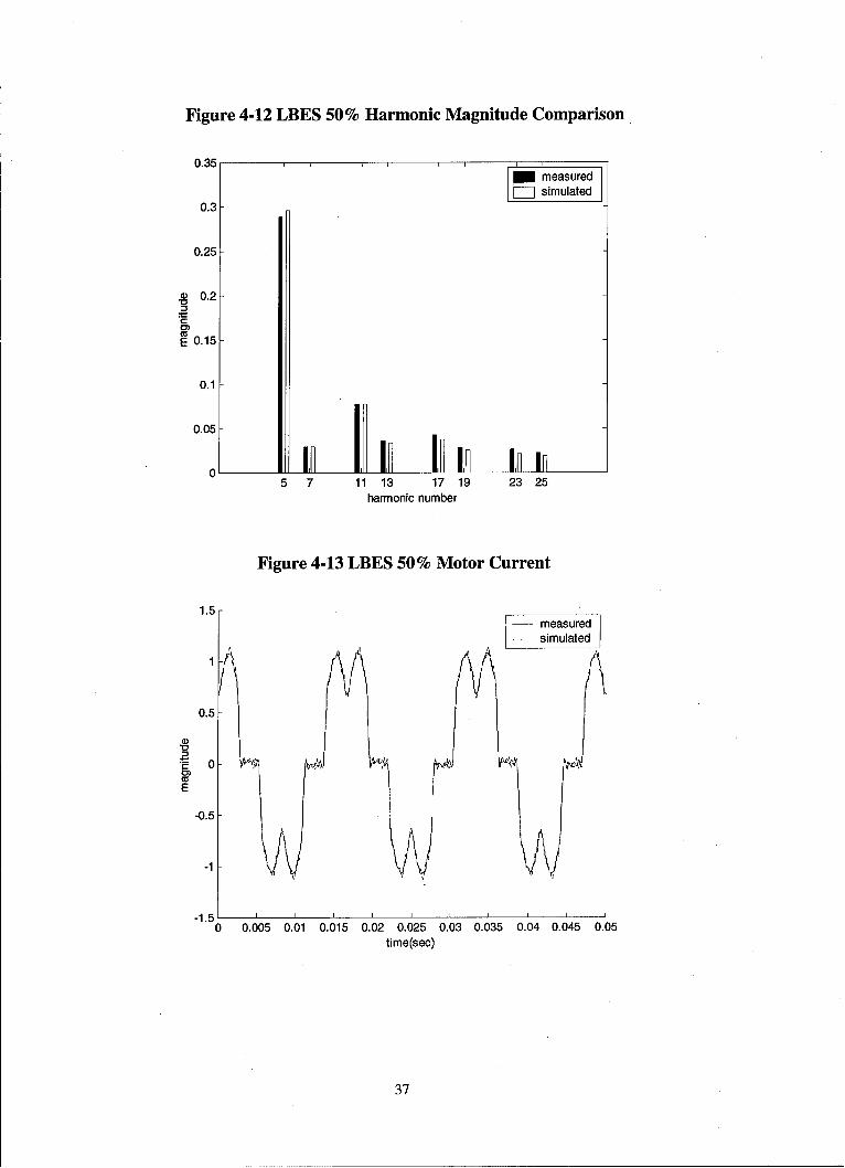
Figure 4-12 LBES 50% Harmonic Magnitude Comparison
0.35 1measured
r simulated0.3
0.25
cD 0.2a
E 0.15
0.1
0.0:-
11 13 17 19 23 25harmonic number
Figure 4-13 LBES 50% Motor Current
1.5- measured
I simulated
0.5
Z!-0)
E
-0.5
-1
- 1 . 5I I I I I I I I I
"0 0.005 0.01 0.015 0.02 0.025 0.03 0.035 0.04 0.045 0.05time(sec)
37

Figure 4-14 LBES 10% Harmonic Magnitude Comparison
0.71measured
[.6 simulated0.6
0.5
D 0.4
E 0.3
0.2
0.1
0 E E UJ, -in fin5 7 11 13 17 19 23 25
harmonic number
Figure 4-15 LBES 10% Motor Current
2- measured
simulated1.5
0.5
E-0.5
-1
-1.5
"-2 I L I I I I I - I I0 0.005 0.01 0.015 0.02 0.025 0.03 0.035 0.04 0.045 0.05
time(sec)
38

Table 4-5 Tabulated LBES Simulation Results
90% Power 50% Power 10% PowerMeasured Simulated Error % Measured Simulated Error % Measured Simulated Error %
1 1 1 1 1 10.2402 0.2456 2.25 0.2896 0.2965 2.38 0.5544 0.593 6.960.0707 0.0691 2.26 0.0293 0.029 1.02 0.2927 0.3116 6.460.0634 0.0649 2.37 0.077 0.0768 0.26 0.0648 0.0588 9.260.0451 0.0415 7.98 0.0354 0.0336 5.08 0.0777 0.0779 0.260.0268 0.0285 6.34 0.0421 0.0381 9.50 0.0181 0.0112 38.120.0248 0.0235 5.24 0.0282 0.0254 9.93 0.0337 0.0276 18.100.0098 0.0105 7.14 0.0266 0.0214 19.55 0.0026 0.0019 26.920.0114 0.0117 2.63 0.0221 0.0188 14.93 0.0155 0.0101 34.8425.63% 26.02% 1.53 29.55% 29.97% 1.42 53.69% 56.10% 4.49
4.3 Harmonic Source Comparison
The final step of model validation consisted of analyzing a simple system shown in Figure
4-16 using the current source injection method as outlined in Chapter 3. This method is highly
accurate when only one harmonic source is present but leads to exaggerated distortion as more
non-linear loads are added. [6] The primary reason for this section was that the previous
validation sections did not include a distribution transformer or additional loading of the system.
The technique outlined in [21] and [6] is well established and establishes a means of comparing
results from the PSCAD simulation.
Figure 4-16 Current Source Comparison Circuit
0.00066667 0.00337iAB17.977 [UMW go, u~ '/-•G
IVmes 1.055 [MVARI
.0OO02448F- A
• , , _c ........., ......... ... ..... .................. ......... .... -4_•.Lra Cv 6 Pulse •I
? t, P
#1 #2 IA ~ 0.2
39

The system impedances of interest in the circuit above are the transformer, load, and generator
phase-to-neutral values. The harmonic currents generated by the six-pulse rectifier flow through
these impedances creating the voltage distortion on the main bus. Testing has shown a consistent
relationship between the negative sequence impedance of rotating machines and the harmonic
impedance. The negative sequence impedance is roughly equivalent to the subtransient reactance
and therefore is used in determining the equivalent harmonic impedance. [21] In the test system
above a subtransient reactance of 20% is used for the generator. The harmonic impedance of the
generator is given by:
Zgen = jXgen = jnXd
Equation 4-2
The transformer and load impedance is estimated in the phase-to-neutral equivalent circuit by
assuming a transformer impedance of 3%. The harmonic impedance of the transformer and load
on the primary side is:
Ztran = .2 V12) + in(0.03{jQI
Equation 4-3
where: V 1 is the primary voltageV2 is the secondary voltageVA is the volt-amp rating of the transformern is the harmonic number
The phase to neutral equivalent circuit of the test system is shown in Figure 4-17, the
calculations are carried out in the MATLAB script included in Appendix A.
40

Figure 4-17 Phase-to-Neutral Equivalent Circuit
DZran '2gen'
The test system was simulated in PSCAD and the harmonic current and harmonic voltage
magnitudes were recorded. The recorded harmonic current magnitudes were then applied to the
phase-to-neutral equivalent circuit. The harmonic voltages up to the 2 5 th harmonic are shown in
Figure 4-18 for the PSCAD simulation and the phase-to-neutral equivalent circuit. It is clear that
the PSCAD simulation has accurately simulated the effects of a transformer and linear load.
Figure 4-18 PSCAD Current Source Comparison
0.12 1- PSCAD
Current Source
0.1
0.08
® 0.06
0.04-
0.02
0C. 11 11511 13 17 19 23 25
Harmonic Number
4.4 Model Validation Summary
The preceding sections demonstrate that this modeling technique accurately reflects
harmonic current and voltage distortion in power systems such as those found on Navy ships.
PSCAD simulations were compared to actual measurements taken on a system equipped with a
ship generator and propulsion motor drive (4.2). Simulations were also compared to established
41

harmonic analysis techniques (4.1 and 4.3). In both cases highly accurate results were obtained.
In the next chapter a more detailed system will be developed that is more representative of an
actual shipboard power system. However, as there is no hardware developed for such a power
system, there are no measurements available at this time for validation purposes. All the
elements of this proposed power system are common with the previous studies that have been
compared to either actual measurements or proven analytical techniques in this chapter.
Therefore, we can be relatively confident in the simulation results of the proposed power system,
even without hardware validation.
42

Chapter 5 Integrated Power System Development
The baseline IPS for this research is developed and analyzed in this chapter. This system is one
approach to an IPS for a future surface combatant and is not intended to be an optimized solution
for any particular ship design. The purpose of the system is to give a realistic picture of
harmonic distortion over the wide operating range of Navy ships.
5.1 Approach and Assumptions
The development of an IPS requires assumptions that define the characteristics of the
system. Changes in these assumptions may affect the results and conclusions of the study. The
entering assumptions for the development of this architecture include:
* 4160 V, three-phase main bus
"* Hybrid Distribution System (Some loads powered from a 450 V bus and some loads
fed from DC load centers connected to the 450 V bus)
"* Generator sets capable of 5-30 MW available for use. Commercially available prime
mover ratings are not considered herein.\
"* Generator subtransient reactance of 20 %
"* Circuit breakers capable of 5000 amps steady state and 63 kA fault current capacity
available. (i.e. Siemens 8BK40)
"* Induction motor drive capable of 30 MW based on scaling of LBES Motor
"* Ship Service Power requirements based on anticipated future surface combatant
requirements
* Propulsion Power requirements based on anticipated future surface combatant
requirements
5.2 System Description
The system developed for this study is shown in Figure 5-1. Simplification of the overall
* system was required due to the limitations of the PSCAD Educational version. This version of
the PSCAD software is limited to 220 electrical nodes. In order to meet this constraint, all ship
service loads were allocated to only two load centers, each with a 4160/450 V transformer. An
actual design would have multiple load centers distributed throughout the ship each with its own
43

transformer. The radar and gun system power requirements were also combined into a single
load and to evaluate the worst-case harmonics were assumed to be fed from a six pulse rectifier.
Four generators, two 10 MW and two 30 MW, and two main motors (30 MW each) were
installed. Finally, loads were split evenly between two halves of the system.
44

Figure 5-1 Baseline IPS
1OW0 30 mw 30M 1wio0M
4180 VE2UR ~ j 4100 V Do
41M245 VTfan&lor
m~hfmer
Radari~un Mtort Drives fbdwA3unCe
4160V Bus
45

5.2.1 Generator
The system generator is the most important component in determining harmonic
distortion characteristics of the system. The generator presents the lowest impedance at
harmonic frequencies. This impedance can be determined from the subtransient reactance (Xd")
of the generator. As discussed in Chapter 4, harmonic voltages are developed across the phase to
neutral system impedance due to harmonic currents generated by non-linear loads. In general for
a given harmonic current content, voltage distortion increases with Xd". This study assumed
Xd" of 20%. This is a typical value for generators of the size used in this study.[13]
A useful model for a synchronous machine is shown in Figure 5-2. This model
represents the effects of rotor currents on the direct and quadrature axis. These are the per unit
equivalent circuits for a synchronous machine with a single damper circuit on both the direct and
quadrature rotor axis. The model terminals are constrained by voltage, assumes sinusoidal
winding distribution, and employs the equal mutuals base system. There are the three phase
windings on the stator and the field, direct, and quadrature windings on the rotor. The direct and
quadrature windings are representations of current paths in the rotor. This machine model
follows the derivation in [25]. In order to analyze this model, the stator variables are shifted to
a reference frame attached to the rotor by the Park's transformation.
cos(9) cos(0 - -) cos(O + -)3 3
T = 2 -sin(6) - sin( -- ) - sin(0 +-2)3 3 3
1/2 1/2 1/2
Equation 5-1
Stator phase quantities are transformed into direct and quadrature quantities as follows:
Vdl ~Va1Vq =T* vb
V0 Vc
Equation 5-2
Phase variables can be recovered from the direct and quadrature quantities using the inverse
transformation.
Currents are used as auxiliary variables as follows:
46

Id- Xd Xad Xad V/IdIik LXd Xkd Xa. x fLd
i Xad Xad Xf J [K.f[iq =[X Xaql-i kq x aq X kqJ
Equation 5-3
And the state equations become:
d -d =OoVd + CO q - O)oraid
dt
Equation 5-4
dtqdt - O°Vq +(cOY/q - Ooraiq
Equation 5-5
dt
Equation 5-6
d~4fkq = (JJorkqikq + O0 V f Euto -
Equation 5-7
dt 2H
Equation 5-8dco _ o)TeTn
dt 2 T
Equation 5-9
dt
Equation 5-10
47

Figure 5-2 Synchronous Machine Transient Model
id if
ra xal 3a k lxf 1 rf +
rk
iq
ra xal+ ,xaq xq
rkq
The model described above provides accurate results in a wide variety of situations.
However, representations such as this are unnecessarily complicated for harmonic distortion
studies and slow simulations considerably.
Harmonic distortion is a steady state phenomenon and therefore does not require the
modeling of machine dynamics; however a modification of the typical steady state machine
model is required for this study. A synchronous machine steady state equivalent circuit is
normally represented as a voltage source behind a synchronous reactance where the synchronous
reactance represents the combined effect or the air gap and leakage components.
48

Figure 5-3 Steady State Synchronous Machine Model
Air Gap Component Leakage Component +
Air Gap Voltage Terminal Voltage
Synchronous= Air gap + Leakage
Terminal Voltage
o
This model would not be adequate for this study in that the synchronous reactance is not the
reactance seen by the harmonic currents. Instead, the generator was modeled as a voltage source
behind subtransient reactance (Xd") in order to accurately model harmonic distortion. The
voltage source allowed for control of voltage, phase angle, and frequency. In situations where
two generators were operating in parallel, one machine was set to automatically maintain bus
voltage while the voltage and phase angle of the other machine were adjusted to ensure proper
distribution of real and reactive power between the two machines.
The sizes of the generators were based on operational cost considerations. The prime
mover for the generator on a surface combatant is a gas turbine engine. Gas turbines operate
inefficiently when lightly loaded. For this reason generator sizing was chosen so that the system
could be operated as much as possible with the generators loaded at 50% power or above. The
power requirements for the future surface combatant are shown in Figure 5-4. A surface
combatant spends the vast majority of its time at sea under cruise loading at speeds of less than
49

15 knots. The power requirements show a consumption of 10 MW with no propulsion power.
This increases to roughly 20 MW at 15 knots. The power requirements dictated installation of
two 10MW generators and two 30 MW generators operated in the following manner. For ship
speeds up to 15 knots the two 10 MW generators would be online in a ring bus configuration.
These generators would both be at 50% loading with no propulsion power required and increased
to full loading at 15 knots. For ship speeds from 15 knots to 25 knots one 30 MW generator
would be added to the ring bus. Finally, for speeds up to 30 knots the final 30 MW generator
would be brought online and the bus would be split. It should be noted that marinized gas
turbines in these power ranges at 4160 V are not in use by the US Navy. While this
configuration allows the online gas turbines to be operated in the most fuel efficient manner, the
costs associated with certifying gas turbine in these power ranges could negate these savings.
Splitting the electric bus for ship speeds above 25 knots is necessary due to circuit
breaker fault current limitations. In addition to determining the harmonic distortion Xd" also
determines the maximum fault current in the case of a short circuit as follows:[ 14]
ISC = VArated
1line Xd
Equation 5-11
In a 4160 V distribution system with Xd" of 20%, the breaker limitation of 63 kA requires
generating capacity on a single bus to be less than 73 MW.
50
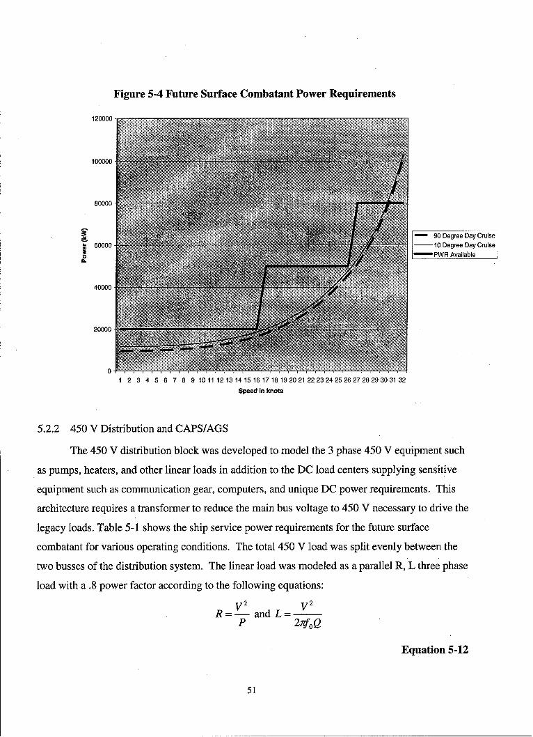
Figure 5-4 Future Surface Combatant Power Requirements
120000
100000.•
80000
F 90 Degree Day Cruise
S60000- - 10 Degree Day Cruise
0 PWR Availablea.
40000
20000
01 2 3 4 5 6 7 8 9 1011 12131415161718192021 22232425262728293031 32
Speed in knots
5.2.2 450 V Distribution and CAPS/AGS
The 450 V distribution block was developed to model the 3 phase 450 V equipment such
as pumps, heaters, and other linear loads in addition to the DC load centers supplying sensitive
equipment such as communication gear, computers, and unique DC power requirements. This
architecture requires a transformer to reduce the main bus voltage to 450 V necessary to drive the
legacy loads. Table 5-1 shows the ship service power requirements for the future surface
combatant for various operating conditions. The total 450 V load was split evenly between the
two busses of the distribution system. The linear load was modeled as a parallel R, L three phase
load with a .8 power factor according to the following equations:
V 2 V 2
R = - and L=vP 2 7fo Q
Equation 5-12
51

To account for worst case conditions, the non-linear load contribution was modeled as a
six pulse rectifier and DC link driving a resistive load. The DC link for this component was
designed for maximum power factor and minimum line current harmonics according to [22].
The script used for calculations of the DC link is included in Appendix A.
The combined array power system (CAPS) and the advanced guns system (AGS) power
requirements were combined. The total power draw was split evenly between the two busses and
was again simulated as a six pulse rectifier with a DC link designed for maximum power factor
and minimum line current harmonics.
Table 5-1 Future Surface Combatant Ship Service Power Requirements
Battle Cruise J Anchor .90 degree 10 Degree 90 Degree 10 Degree 90 Degree 10 Degree
CAPS/AGSKW 3500 4500 2800 3700 800 1300450 V Linear(• 5300 7700 5100 6300 2300 340045OV Non Linear (K\A 1800 1800 1600 1600 700 7004.5 0 ,.V .,.,._o ~n ..L_-----( -. ....... -- -------- 0 0--- ............... ------ -.... ---_.0. -...... ------..... . 7 0 _ ,....._7 0
,Total (KW) 10600 14000 95001 11600 3800n 5400
5.2.3 Six Pulse Induction Motor Drive
The induction motor drive was modeled using the same parameters contained in 4.2.3.
52

Chapter 6 Baseline Simulations and Mitigation Techniques
This system described in Chapter 5 was simulated for ship speeds of 0, 15, 25, and 30 knots
under each of the loading conditions listed in Table 5-1. The following parameters were
measured:
* 450 V bus
o Magnitude and phase of individual voltage harmonics
o THD
* Generators
o Magnitude and phase of individual current harmonics
o THD
The results were compared to the requirements of MIL-STD-1399, IEEE STD 45-1998
Recommended Practices for Installation of Electric Installations on Shipboard, and IEEE STD
519- 1992, Recommended Practices and Requirements for Harmonic Control in Electrical Power
Systems. MIL-STD-1399 and IEEE STD 45-1998 require THD for voltage not to exceed 5%
with individual harmonic distortion less than 3%. These requirements are the same as those
recommended in IEEE STD 519-1992 for general systems. Recommendations for dedicated
systems in IEEE STD 519-1992 allows for up to 10% voltage THD. The more stringent
requirements of MIL-STD 1399 and IEEE STD 45-1998 are based on protecting sensitive
equipment such as communications and weapons systems. In an IPS system, this sensitive
equipment is isolated form the distortion on the main bus by a rectifier and inverter. As long as
the front end rectifier is designed to operate off of a bus with higher distortion levels the
sensitive equipment should not be effected. In that motors and generators are normally rated with
a consideration of 10% harmonic content (NEMA MG-1), the higher distortion limits of IEEE
Std 519-1992 for dedicated systems should be adequate for the 450 V bus.
Setting a limit for current harmonics is more complicated than for the voltage harmonics.
MIL-STD-1399 places the responsibility on the user equipment and its effect on the system bus.
60 Hz equipment of 1 kVA or more "shall not cause single harmonic line currents to be
generated that are more than 3% of the unit's full rated load fundamental current". This
requirement will be difficult to meet without extensive filtering or unnecessarily increasing the
size and complexity of all electronic interfaces. Table 6-1 shows the IEEE STD 519 harmonic
current profile for a six pulse converter. Every harmonic up to the 19th violates the requirements
53

of MIL-STD-1399. MIL-STD-1399 was written with segregated power systems in mind where
the relatively small generators (2.5 MW on a typical surface combatant) are more easily affected
by ship service loads. On an IPS ship, the only load that draws enough harmonic current to
significantly affect the bus voltage profile is the propulsion motor drive.
Table 6-1 IEEE STD 519 Harmonic Current Profile
Harmonic c.u. of Fundamental1 15 0.1927 0.13211 0.07313 0.05717 0.03519 0.02723 0.0225 0.016
The philosophy of IEEE STD 519-1992 is to limit harmonic injection from individual
consumers in order to prevent voltage distortion that violates the previously stated limits. It is
not realistic to apply the limits of IEEE STD 519-1992 to an IPS due to the differences in system
characteristics between the terrestrial grid and an IPS. The limits imposed by IEEE STD 519-
1992 are meant to control a wide number of customers all connected to the same power source.
In an IPS, the Navy directly controls all pieces of equipment attached to the main bus and can
more accurately predict the effect of each component on overall system performance. As long as
the overall voltage distortion remains in specification the system will function properly.
Another complication in trying to set current distortion limits in the same way as the
voltage distortion limits were set is that high current distortion does not necessarily result in high
voltage distortion. The motor drive (LBES 19 MW) with a six pulse rectifier front end will be
used to illustrate this point. Figure 6-1 and Figure 6-2 show the voltage and current on the AC
side of the pulse width modulated (PWM) motor drive (the voltage in Figure 6-1 has been scaled
to allow plotting on the same graph). At 10% power the current distortion is 67% and the
voltage distortion is 4.8%. At 90% power the current distortion is 26% and the voltage distortion
is 16.8%. The higher current distortion at 10% power does not lead to high voltage distortion
because the magnitude of the harmonic current is small due to the lower power demand. The
high current distortion at low powers is a characteristic of PWM motor drives. This
54

characteristic is due to a large capacitor in the DC link. Current only flows when the output of
the rectifier is higher than that of the capacitor. At light loads, the ac side current is
discontinuous and only becomes continuous as load on the DC link increases.
For the reasons listed above it makes sense to establish current distortion limits based on
the ratings of the generators. The fifth and seventh harmonic current limits for the generator
installed at LBES are 9% and 8% of the fundamental limit. [23] NEMA MG-I allows for 10%
voltage distortion in the ratings of machines suggesting that higher current distortion levels are
acceptable. For the purpose of this study the LBES generator limits will be used as a benchmark
for acceptable levels of current distortion. Table 6-2 shows the current limits for the generators
used in this study.
Table 6-2 Generator Current Ratings
10 MW Generator 30 MW Generator
Fundamental Current Limit 1734 A 5204 A
5 th Harmonic Current Limit 156 A 468 A
7th Harmonic Current Limit 138 A 416 A
55

Figure 6-1 Voltage and Current 10% Power
Main: Graphs2 Volt line to lIne " 1la PMM-I >2.0
1.50- Motor Current1.00-
0.50'
0.00-
-0,50
-1.50 Bus Voltagei• -2,00 -!_. . .. .
0.4700 0.4750 0.4600 0.4650 0.4600 0,4650 0.5000 0.5050 0.5100
Figure 6-2 Voltage and Current 90% Power
Main: Graphs
* Volt line to line M "la PMM-1 >8.0. . .
6.0 Motor Current4.0
2.0-
0.0
-2.0-
-4.0-
-8.0-8.0. Bus Voltage
0.4150 0.4200 0.4250 0.4300 0.4350 0.4400 0.4450 0.4500 0.4550 0.4600
6.1.1 THD on the 450 V bus
The most important simulation results concern the voltage distortion on the 450 V bus.
Figure 6-3 shows THD on the 450 V bus for each of the simulation cases. The baseline six pulse
system violates MIL-STD 1399 and the guidelines of IEEE 519-1992 for dedicated systems for
all loading conditions and ship speeds simulated when the propulsion motors are operating. The
56

voltage distortion meets both criteria without the propulsion engines operating (the 0 knot series
of Figure 6-3). Typically, you would expect that as propulsion power increases so would voltage
distortion due to the increased magnitude of the harmonic currents. In these simulations this is
the case but only within the discrete generator operating configurations. For example, at 15
knots both 10 MW generators are operating at full power. If an 18 knot ship speed is desired, the
30 MW generator must be brought onto the bus in order to supply this additional power. The
addition of the 30 MW generator reduces the phase to neutral system harmonic impedance and
possibly reduces the overall system voltage distortion despite the additional harmonic current
from the power increase
In the baseline IPS simulation the highest distortion occurs at 25 knots. However, the
distortion level is only slightly higher than the 15 and 30 knot conditions. The 15, 25, and 30
knot speeds correspond to the maximum propulsion power for a given generator configuration
and therefore the highest. voltage distortion in each configuration. Even though propulsion power
(and harmonic current magnitude) more than doubles between the 15 and 25 knot conditions,
and again between the 25 and 30 knot conditions, THD(voltage) remains relatively constant due
to the decrease in system harmonic impedance from the additional power generation capability
brought online to meet the propulsion demand.
Figure 6-3 also illustrates that the distortion level of the power system is not significantly
influenced by changes in loads other than the propulsion motor. The cruise loading condition on
a 90 degree day is the condition with the least amount of non propulsion load and results in the
worst case distortion for the system but only by a marginal amount. This is particularly true at
the highest propulsion motor powers. Table 5-1 shows that there is almost a 5 MW difference in
ship service loading between the 90 degree cruise condition and the 10 degree battle condition.
At full propulsion power this additional load reduces total distortion by only 0.3 %. At 15 knots,
where the total propulsion power (6 MW) is less than ship service loads, the reduction in
distortion is 2%.
57

Figure 6-3 THD 450 V Baseline System
16
14 4
12
10
E Cruise 90'
0ICruise 11" 8" Tg d Battle 90
c r oBattne 10
6
4.
2-
0 15 25 30
Ship Speed (knots)
The 90 degree, cruise loading condition was chosen to conduct a more detailed look at
THD over the entire propulsion motor loading range. As mentioned in the preceding paragraph,
this was the loading condition the rasitin twen the stdistortion levels. It can be assumedthat the other loading conditions would exhibit a similar response over the operating range but at
slightly lower distortion levels. Figure 6-4 shows the voltage distortion from 0 knots to 30
knots. The three curves represent the discrete electric plant configurations. The threeconfigurations are:
"• Two 10 MW generators in parallel on a ring bus (0-15 knots)
"• Two 10 MW and one 30 MW generators in parallel on a ring bus (15-25 knots)
"• Split plant with a 10 MW and 30 MW generator on each side (25-30 knots)
The drop in distortion levels at the transitions between the configurations is evident. The lower
generator impedance results in lower distortion levels. The figure also shows that the voltage
58

distortion levels meet IEEE Std 519-1992 at speeds less than 13 knots. This is significant in that
navy ships spend 90% of their time at sea at speeds less than 13 knots.
Figure 6-4 THD vs Speed, Cruise Loading, 90 degree day
18-
16 -- - -- - - -
1210
-"e"Rlng Bus 2X1OMW
-1" -Ring Bus 2X1OMW + 30MW
--*-SplIt Plant 2XIOMW 2X30MW
8 - Limit
6 :
4
2-
0 1 2 3 4 5 6 7 8 9101112131415161718192021 222324252627282930
Speed (knots)
The individual harmonic components for each speed and loading case are shown in
Figure 6-5 through Figure 6-8. The figures show that the fifth and seventh harmonics are the
major contributors to the voltage distortion. These harmonics violate MIL-STD- 1399 in every
simulation except for the 0 knot simulation. Tabulated results of the baseline simulations are
included in Appendix C.
59

Figure 6-5 Individual Harmonic Voltages, Cruise Loading, 90 degrees
14
12"
, Ag
57 11 13 17 19 23 25
Harmonic Number
Figure 6-6 Individual Harmonic Voltages, Cruise Loading, 10 Degrees
025knots
030 knots
"4~
2"-
0-
5 7 11 13 17 19 23 25
Harmonic Number
60
: i i i U.

Figure 6-7 Individual Harmonic Voltages, Battle Loading, 10 degrees
12-
10-
8-
rU-
o ~02 knots030 knots
0
5 7 11 13 17 19 23 25
Harmonic Number
Figure 6-8 Individual Harmonic Voltages, Battle Loading, 10 degrees
12
10--
:EQ0 knotsiSknt s1, knots
5 7 11 13 17 19 23 ' 25Harmonic Number
61

6.1.2 Generator Current Distortion
The individual harmonic current magnitudes for the 90 degree day cruise loading
conditions are shown for each generator in Figure 6-9 and Figure 6-10. As with the voltage
distortion, the ship service loading had little effect on the overall results for current distortion.
The results for the other loading conditions were similar. Tabulated results of all baseline
simulations are included in Appendix C. The fifth harmonic current limit for the 10 MW
generator and the 30 MW generator is 156 A and 468 A respectively. The seventh harmonic
current limits are 138 A and 416 A. The baseline system violates the fifth harmonic limit for
both the 10 MW generator and the 30 MW generator at the 25 and 30 knot speeds. The seventh
harmonic is within the limit for all cases.
Figure 6-9 Harmonic Current Magnitude (RMS) 10 MW Generator200
180
160"
140 -"1ý4
120 "J
MO knotsR15 knots125 knots
= 130 knotsU 80
40.
20- 4
5 7 11 13 17 19 23 25
Harmonic Number
62

Figure 6-10 Harmonic Current Magnitude (RMS) 30 MW Generator
600 -
500
400 . -- -- - -
300 kn.
1030 knt
200--
5 1 13 17 19 23 25
Harmonic Number
6.1.3 Baseline Simulation Conclusions
The baseline IPS with a six pulse motor drive results in unacceptable voltage distortion
and current distortion levels which could cause overheating of rotating machinery such as the
main generators and various shipboard loads. While the voltage distortion levels are high for
speeds above 13 knots, the system operates within the guidelines of IEEE Std 519-1992 for
sp eeds less than 13 knots. The generator current data suggests that the majority of the distortion
is caused by the fifth and seventh harmonic. Figure 6-11 shows the 30 MW generator current
for the 10 degree day loading condition and the ship at 25 knots. This waveform was generated
in a MATLAB script (Appendix A) from the magnitude and phases of the individual harmonic
components. In Figure 6-12 the generator current waveform was generated with the fifth and
seventh harmonic removed. The improvement in THD suggests that if the fifth and seventh
harmonics were attenuated a design which meets the established criteria for voltage and current
could be achieved. In the following section methods of removing these harmonics will be
investigated.
63

Figure 6-11 Generator Current, 10 deg day, 25 knots
THD =25.1951%1.5
0.5-
.E 0"5n
U)M
":3
C-
E
-0.5
-1
-1.5 I - I I0 0.005 0.01 0.015 0.02 0.025 0.03 0.035
time(sec)
Figure 6-12 Generator Current, 10 deg day, 25 knots, 5th and 7th Harmonics Removed
THD =10.4033%1.5
1
0.5
U-
CUE
-0.5
-1
-1.5 I I I0 0.005 0.01 0.015 0.02 0.025 0.03 0.035
time(sec)
64

6.2 Harmonic Distortion Mitigation Techniques
The results of Chapter 6 clearly indicate that in order to implement an IPS with this
configuration the harmonic current magnitudes at the fifth and seventh harmonics must be
reduced. There are three methods employed in industrial and commercial power systems to
reduce the flow of harmonic currents. These are: [24]
"* Use of shunt filters
"* Use of multipulse power converters
"* Harmonic current injection
In this section the first two methods of attenuation listed above will be simulated in order
to obtain system results. In addition to these two methods a modification to the operation of the
propulsion motor drive will also be simulated.
6.2.1 Line Commutated Rectifier Motor Drive
Section 4.2.3 describes the operation of the propulsion motor drive used in the simulation.
As mentioned earlier, this is a phase controlled converter whose firing angle is controlled as
shown in Figure 6-13. The firing angle of the converter is controlled to maintain stability on the
DC link between the rectifier stage and inverter stage of the motor drive circuit. One
consequence of controlling DC link voltage in this manner is that it degrades the power factor of
the motor drive. The relationship between power factor and THD is established in Equation 2-11
through Equation 2-14. In general, the power factor of the converter decreases with increasing
alpha. [9]
65

Figure 6-13 Propulsion Motor Firing Angle
5045
35
' 25S20 ý" 15-
10 -
5-.
0 0.1 0.2 0.3 0.4 0.5 0.6 0.7 0.8 0.9 1
Speed (per unit)
The system was simulated with the motor drive rectifier operating as a line commutated
rectifier by setting the firing angle of the bridge thyristors to zero degrees. Operating the
rectifier in this manner will result in lower harmonic distortion. The 90 degree day cruise
loading condition was used in the model and propulsion loads up to 30 knots were simulated.
The results are shown in Figure 6-14. As expected, operating the front end rectifier as a line
commutated converter significantly reduces the voltage distortion of the system. The limits of
IEEE Std 519-1992 are only exceeded at the highest propulsion loads for the last two electric
plant configurations. Figure 6-15 shows the individual harmonic contribution for the line
commutated and the phase controlled propulsion motor drive of the baseline system simulated
with 90 degree day cruise loading at 30 knots. A marked reduction in the fifth and seventh
harmonic is noticed.
66
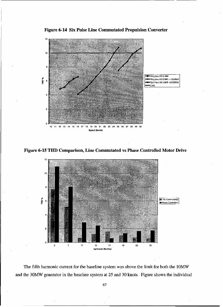
Figure 6-14 Six Pulse Line Commutated Propulsion Converter
12.
10.
"B'Ring Bus 2X10 MW
-*-Ring Bus 2XIOMW + IX3OMW-6'-Spit Plant 2XIOMW +2X3OMW
4-
2-
10 11 12 13 14 15 16 17 18 19 20 21 22 23 24 25 26 27 28 29 30
Speed (knots)
Figure 6-15 THD Comparison, Line Commutated vs Phase Controlled Motor Drive
10
80.
U Line Commutated
mU Phase Controlled
2-A
05 7 11 13 17 19 23 25
Harmonic Number
The fifth harmonic current for the baseline system was above the limit for both the IOMW
and the 30MW generator in the baseline system at 25 and 30 knots. Figure shows the individual
67

harmonic current magnitudes at 25 and 30 knots for the baseline and the line commutated
system. The fifth harmonic is now less than the limit for both generators. (156 A -10MW, 468 A
-30 MW) Tabulated results of the simulations are contained in Appendix C Table 8-7.
Figure 6-16 Individual Harmonic Current (10 MW Generator)
200 - , ' , 7ý -ý -- --- - --
180-
140
S120025 knott 30 knot
025 knot baseline system0 30 knot baseline system
80
60.
40-
20--
0
5 7 11 13 17 19 23 25Hamnonlc Number
Figure 6-17 Individual Harmonic Current (30 MW Generator)
600•
500 X-
400
025 knot/30 knot
0025 knot baseline system030 knot baseline system
200
1000-
0-11
5 7 11 13 17 19 23 25
Harmonic Number
68

6.2.2 Multipulse Motor Drive and Harmonic Filter Systems
The two methods most commonly used to reduce harmonics on power systems are the
addition of shunt harmonic filters and/or the use of a multipulse converter. The baseline system
described in 5.2 was modified to incorporate these two methods of harmonic mitigation. Each
method was implemented separately.
The fifth harmonic filter described in 4.2.2 was used as the basis of the filter designed for
this simulation. The resonant frequency of the filter is given by:1
Equation 6-1
Where f. is the resonant frequencyL is the inductance of the filterC is the capacitance of the filter
IEEE Std 141-1993 recommends the following steps in the design of a filter for harmonic
mitigation.
"* Selection of a capacitor value based on power factor improvement
"* Design an inductor to series tune the capacitor to the desired harmonic
"* Calculate peak voltage and current in order to select components
This method is not suitable for an IPS due to the wide range of reactive load experienced by the
power system. The capacitor selection step presumes that the amount of MVar is known and
relatively steady. In the baseline system of 5.2 the system MVar increases for 7 to 38 when
propulsion power increases from 0 to 100%. Designing a filter for the 38 MVar at full power
would be far too large for normal operations and would be larger than needed to reduce
distortion within limits. Due to space consideration on ships, the ideal filter is the smallest filter
that reduces distortion limits to within specifications.
The capacitor in the filter injects reactive power according to the following equation:
kV 2
M var,=-VXC
Equation 6-2
The LBES uses a 282uF capacitor rated at 2900V for the fifth harmonic filter. Equation 6-2 tells
us that this filter will inject 1.83 MVar. The inductor necessary to tune the filter to the fifth
69

harmonic is lmH according to equation 5-3. This filter was added to the input to the propulsion
motor drive of the baseline system in order to reduce the fifth harmonic.
The 12 pulse motor drive was derived from the LBES motor drive of 4.2.3. Two six pulse
rectifiers can be combined to produce twelve pulse operation if the ac input signal to one rectifier
is phase shifted by 300. The phase shift is accomplished by use of transformer connections and
shown Figure 6-18. One transformer is connected wye-wye while the other is connected delta-
wye. The delta-wye connection produces the necessary phase shift and the combination of the
two transformers produce six phases necessary for 12 pulse operation. The currents of interest
are shown in Figure 6-19. The current Iwye is the normal six pulse input current. The current
Idelta contains no triple-n harmonics due to the delta connection of the transformer. The line
current Iline is the sum of Iwye and Idelta and results in a waveform where the fifth and seventh
harmonics are cancelled. The first non-zero harmonic present in the line current is the 11 th.
Figure 6-18 12 Pulse Converter
70
70

Figure 6-19 12 Pulse Line Current
I0 Ig Ilt
300.00
200.00 -- - - - -- - - - line -- - - - - - - - - - - -- - - --,- - - - - - - - - - - -
100.00
-200.00 1
0.00 5.00 10.00 15.00 20.00Time (ms)
Simulations for the 15, 25, and 30 knot speeds with the 90 degree day cruise loading
condition were performed for the baseline system with the harmonic filter addition and the
baseline system with a 12 pulse motor drive. Both of the alterations reduced voltage distortion
levels to within the limits of IEEE Std 519-1992. Figure 6-20 shows a comparison of the
distortion levels for the baseline system compared to the filter system and the 12 pulse motor
drive system. Figure 6-21 and Figure 6-22 show the THD for the filter system and 12 pulse
system over the operating range of the ship. Tabulated results are contained in Appendix C,
Table 8-8 and Table 8-9.
71

Figure 6-20 THD Comparison
SUBaseline System
E312 Pulse System
15 25 30Speed (knots)
Figure 6-21 Filter System THD
-4RIg Bus 2X10MWURing Bus 2XIOMW + 1X30MW
ooo- -Spft Plent 2510MW + 2X30MWLimit
10 11 12 12 14 15 15' 17 15 19 20 21 22 23 24 25 26 27 28 25 30Speed (knots)
72

Figure 6-22 THD 12 Pulse System
12
10
8'
0 6-ies
~ <~ 'A Serles
4-
2-
10 11 12 13 14 15 16 17 18 19 20 21 22 23 24 25 26 27 28 29 30
Sp.ed (knots)
The individual harmonic voltages are plotted as a percent of the fundamental in Figure 6-23
and Figure 6-24 the 12 pulse and the filter system respectively. The fifth and seventh harmonics
have almost been eliminated in the 12 pulse system as expected. They are still present due to the
fact that the DC load centers and AGS/CAPS system still draw fifth and seventh harmonic. In
the filter system, the fifth harmonic is the only harmonic which has been significantly reduced
due to the design of filter. However, as mentioned above this attenuation is enough to bring the
system to within the limits of IEEE Std 519-1992 for dedicated systems.
73

Figure 6-23 Individual Distortion 12 Pulse System
7 57
6-
€4
Harmonic Number
Figure 6-24 Individual Distortion, Filter SystemEl nots
5.
"3-
0 I
5 7 11 13 17 19 23 25
Harmonic Number
74
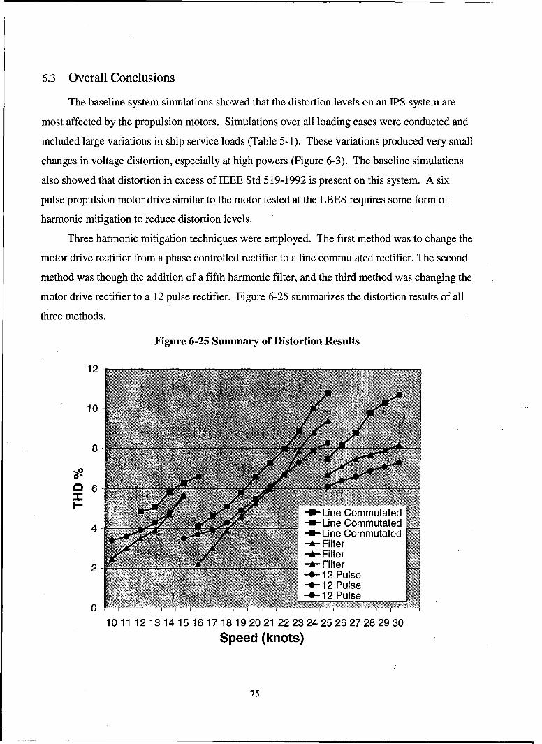
6.3 Overall Conclusions
The baseline system simulations showed that the distortion levels on an IPS system are
most affected by the propulsion motors. Simulations over all loading cases were conducted and
included large variations in ship service loads (Table 5-1). These variations produced very small
changes in voltage distortion, especially at high powers (Figure 6-3). The baseline simulations
also showed that distortion in excess of IEEE Std 519-1992 is present on this system. A six
pulse propulsion motor drive similar to the motor tested at the LBES requires some form of
harmonic mitigation to reduce distortion levels.
Three harmonic mitigation techniques were employed. The first method was to change the
motor drive rectifier from a phase controlled rectifier to a line commutated rectifier. The second
method was though the addition of a fifth harmonic filter, and the third method was changing the
motor drive rectifier to a 12 pulse rectifier. Figure 6-25 summarizes the distortion results of all
three methods.
Figure 6-25 Summary of Distortion Results
12 -
10
8
6 6
l,- -*- Line Commutated-*Line Commutated
44 -' "
4-A- Line Commutated-* Filter-A Filter
2 Filter÷12 Pulse÷12 Pulse
--w12 Pulse0 - -
10 11 12 13 14 15 16 17 18 19 20 21 22 23 2425 2627 2829 30Speed (knots)
75

All three methods significantly reduce distortion. The line commutated rectifier
simulations show that while IEEE Std 519-1992 is exceeded between 24 and 25 knots and again
between 29-30 knots the margin is so small that this system should still be considered for
implementation. Operational procedures could address the distortion levels between 24 and 25
knots. For instance, procedures could dictate shifting to split plant earlier in order to reduce
system impedance and also distortion. The distortion at top speed may not even be an issue due
to the limited amount of time a ship spends at flank speed. Component failure due to high
distortion levels is not an immediate event, degradation takes place over time. Terrestrial
distortion limits already allow for short periods of distortion in excess of the limits. This system
would have the least impact on the ship as it does not require installation of a filter or a
transformer. Additionally, the motor drive would be less complicated due to the fact that
thryristor firing angle control would no longer be necessary. For these reasons the line
commutated rectifier systems should be further investigated. The filter system and the 12 pulse
system both reduced distortion levels to less than IEEE 519-1992 and also reduced the fifth and
seventh harmonics to less than the generator limits. Either of these systems could be
implemented, however, the 12 pulse system includes a significant size and weight penalty. The
two systems differ only in that the 12 pulse system would require two phase shifting
transformers for each of the motor drive while the filter system would require installation of a
single three phase filter at the input to each motor drive. The total component weights are shown
in Table 4-1. These weights were determined based on transformer power densities obtained
from [14], and the size and weight of the fifth harmonic filter at LBES. Based on the size and
weight of the two systems the filter system would be preferable to the 12 pulse system.
Table 6-3 Size and Weight of Harmonic Filter and Propulsion Transformers
Harmonic Filters Propulsion Transformers
Area (M 2) 19.3 94.9
Volume (m3) 41.3 213.8
Weight (mton) 8.3 172.4
76

Chapter 7 Subtransient Reactance
To this point in this research a subtransient reactance of 20% has been assumed. This a typical
value for generators of this size but variations do exist. ABB Marine and Turbo charging quotes
generator subtransient reactance as low as 10% in their project guide for Azipod propulsion
units. As discussed earlier, the subtransient reactance of the generator is the dominant
impedance seen by harmonic currents in the system. Higher subtransient reactance will lead to
higher voltage distortion for a given harmonic current environment. Subtransient reactance also
determines the maximum initial generator current when the generator is subjected to a three
phase fault. Increasing subtransient reactance lowers initial fault current levels but also increases
voltage distortion. Understanding the nature of this tradeoff as it pertains to the IPS described so
far is the purpose of this chapter.
7.1 Fault Current
The current sourced by a generator subjected to a sudden three phase short circuit can be
described over three time periods; subtransient, transient, and steady state. The magnitude of the
current sourced by the generator is a damped sinusoidal whose initial amplitude is limited by the
subtransient reactance during the first few cycles after the short circuit. During the transient and
steady state time periods the amplitude is limited by the transient reactance and synchronous
reactance of the machine. The transient reactance of the generator is associated with the field
winding on the rotor and the subtransient reactance is associated with additional current paths on
the rotor of the machine. The damping of the response is associated with the resistance of these
current paths. For a given generator this current can be predicted by solving Equation 7-1.
Figure 8 shows the response of a generator with 25% and 15% subtransient reactance to a sudden
three phase fault. The lower subtransient reactance results in significantly higher initial current.1 l(
{I+t.1 1 $ e cos(OX)X d X d Xd Xd X
Equation 7-1
Where:Ta = armature time constant
77

Td' = transient time constantTd" = subtransient time constantXd = synchronous d axis reactanceXd' = transient d axis reactanceXd" = subtransient d axis reactance
Figure 7-1 Generator Fault Current
14--- 25% subtransient reactance12- 15% subtransient reactance12
10
8-
S6 i
o.. . .. .
nI)II I i
CD I I
4~ 4 I I
I
-2 1 1
0 0.05 0.1 0.15 0.2 0.25time (sec)
When choosing a low or medium voltage system for a ship IPS, the current handling capabilities
of available circuit breakers can easily be exceeded. Without going through a product
development for a specialized breaker or employing fault current limiters, the ratings of the
circuit breaker with the highest current handling capabilities are 5000 amps steady state and
63kA fault. These ratings limit the power handling capability of the electrical bus as follows.
Equation 5-11, repeated below, determines the fault current for a given bus voltage, generator
subtransient reactance, and power capability. Figure 7-2 shows the fault current expected for
subtransient reactances of 15%, 20%, and 25%. At 15%, the 63kA breaker rating is exceeded at
approximately 55 MW, limiting the power handling capability of the electrical bus.
78

= VArated
Figure 7-2 Generator Fault Current vs. Installed Power
100
90
80
•"70-
60
ca 50
40
30
20 -''''40 45 50 55 60 65 70 75 80
Installed Power (MW)
7.2 Voltage Distortion
A higher value of subtransient reactance is desirable to support higher power demands on an
electrical bus but this leads to increased voltage distortion. In order to gain an understanding of
the effect of subtransient reactance on voltage distortion the circuit in Figure 7-3 was
constructed. The circuit consists of a single 20MW generator supplying the propulsion motor
drive of section 4.2.3. Generator subtransient reactance was varied from 15%-25% and the
propulsion motor drive was simulated at powers from 2MW to 20MW. Voltage and current
distortion were measured and results are plotted in Figure 7-4, Figure 7-5, and Figure 7-6. The
data shows that voltage distortion is significantly effected by the subtransient reactance value.
Figure 7-6 shows that at low motor power, where the harmonic current magnitudes are small, the
difference in the resulting voltage distortion is relatively small. However, as the drive power
79

increases, the effect of the subtransient reactance on voltage distortion is clearly evident,
resulting in increases of distortion levels on the order of 15%. The effect of the DC link voltage
control is also clearly evident in this simulation. We see the voltage distortion decrease
significantly as the thyristor firing angle is decreased at the higher power levels.
Figure 7-3 Subtransient Reactance Simulation Circuit
<1110<
oto
Drive
80

Figure 7-4 Voltage Distortion
40 - -
30--
02
100
subtransient reactance (pu) 0.5 0propulsion drive power (MW)
Figure 7-5 Current Distortion
40 -I-
20'0.2
20
subtransient reactance (pu) 0.5 0propulsion drive power (MW)
81

Figure 7-6 Voltage Distortion vs Motor Drive Power
40-
25%
35
30"
25-
0 20-1-
15
10
5
02 4 6 8 10 12 14 16 18 20
propulsion drive power (MW)
7.3 Impact on the Baseline System
When the baseline system was developed a subtransient reactance of 20% was chosen because
this was a typical value for marine generators. This selection resulted in the requirement of
splitting the main bus in order to supply the full 80MW of power. A more practical approach
when designing an IPS would be to set a minimum subtransient reactance for the generators
based on the power of each bus. In the case of the baseline system if we limited subtransient
reactance to no less than 22% we would be able to provide the entire 80MW of power from a
single bus. The 12 pulse system simulations for the 90 degree cruise loading were repeated with
the 22% subtransient reactance and plotted over the results from the earlier simulations. The
increase in subtransient reactance results in an increase in THD on the order of 1-2 %. The slight
increase in distortion is more than offset by the operational flexibility gained with the higher
subtransient reactance. Figure 7-7 shows the results. Conversely, you could limit the power on
82

each bus in order to accommodate a lower subtransient reactance. Limiting power to 40 MW on
each bus and operating with a subtransient reactance of 15% could allow operation without a
harmonic filter or a 12 pulse system. The worst case distortion for the baseline system (six pulse
motor drive without harmonic filter) drops to 10% if subtransient reactance is lowered to 15%.
Figure 7-7 THD % with 22% Subtransient Reactance
10
10 11 12 13 14 15 16 17 18 19 20 21 22 23 24 25 26 27 2 3 30
Speed (knots)
83

This page intentionally left blank.
84

Chapter 8 Conclusions
Commitment to powering future Navy ships with IPS requires an understanding of the effect
on system power quality of the components of the system. In this research an attempt was made
to quantify the distortion characteristics of an IPS that might be used on naval surface
combatants. The power requirements of the future surface combatant were simulated in order to
present a realistic picture of propulsion and ship service demand and components tested at LBES
were simulated in order to validate the modeling techniques used in this research. The results of
the analysis illustrate some of the tradeoffs necessary in formulating an IPS for a navy ship.
Additionally, these results also show some of the system characteristics necessary to provide
adequate power quality in an IPS.
The first conclusion of this research is based on the premise that power requirements for the
navy ships of the future will continue to grow. With this premise in mind, system voltage of
4160 is too low to service the power needs of future navy ships using electric propulsion. The
primary benefit of the 4160 V system is that step-down transformers are not required at the
interface of the rectifier and system bus. While this presents a significant savings in size and
weight, future high energy weapons will demand power beyond the capabilities of a 4160 V
system. Chapter 7 showed the relationship between subtransient reactance and fault current. It
would be necessary to increase the subtransient reactance of installed generators in order to
provide additional power but this increase would also have a negative impact on the system
power quality. Chapter 6 showed that THD was within the limits of IEEE Std 519-1992 for the
80 MW system, however, increasing the power capability of the system would also increase the
harmonic current level. The increase in harmonic currents coupled with the higher subtransient
reactance would raise THD above the 10% limit. At 80 MW, a 4160 V system is already at the
limits of its power handling capabilities. Selecting this voltage level would limit the prospects
for incorporation of the high energy weapons expected in the future.
The first advantage of an IPS arrangement, listed in Chapter 1, was "increased fuel economy
due to the efficient operation of the prime mover". This true in that with an IPS the ship is no
longer using a large gas turbine (operating at a fraction of its rating when the ship is at less than
flank speed) for propulsion and additional gas turbines to supply ship service power
85

requirements. In theory, with an IPS, fuel efficiency savings will garnered by using the same
prime mover to supply propulsion as well as electrical power requirement. In the baseline
system of Chapter 6 the generator sizes of 10 MW and 30 MW were selected in order to
efficiently operate the prime movers. The selection was based on the following:
* A minimum of two generator sets will be operating in order to have a redundancy
* Gas turbines operate inefficiently a light loads, below 50%
These statements resulted in the generator selection above and an operational philosophy where
the two 10 MW generators would be normally operated and ship speeds below 15 knots. When
higher speeds were necessary the 30 MW generators would be brought online. Since navy ships
spend the majority of their time at speeds below 15 knots, the system would normally operate
with its smaller prime movers online and each loaded at 50% rated power or above. However, if
we examine the available turbine/generator sets we find that much of this efficiency is lost due to
a lack of sets in the desired power range. Table 8-1 shows the turbine/generator sets are available
for use in an IPS. The limited selection would result in an 80 MW system with either four
LM2500 propulsion generators or three LM 2500+ generators and a single DDA 501-K34G.
Both cases result in excess generation capacity at speeds less than 15 knots, which would affect
the efficiency of operation over the lifetime of the ship. At a system voltage of 13.8 kV the loss
of efficiency is even greater. An 80 MW IPS would require the installation of two RR MT-30
and two GE LM500. The two smaller generators are unable to supply even the non-propulsion
loads, so in order to supply redundancy, both of the large generators would be required to be
operating at all times. The small generators would only be placed online in order to reach flank
speed. This configuration is the opposite of what is desired for efficient operation of the prime
movers. A turbine/generator set with a power rating on the order of 10 MW is required to fully
capture the efficiency inherent in an IPS.
Table 8-1 Turbine/Generator Sets
[Engine JVoltage(kV) JPower(MW)GE LM2500 4.16 21GE LM2500 + 4.16 26DDA 501-K34G 4.16 3
[RR MT-30 13.8 36.25GE LM500 13.8 3.8
86

The last conclusion of this research is that harmonic mitigation techniques exist that
would allow the supply of non-sensitive AC loads from transformers connected directly to the
main bus of an IPS with electric propulsion. It was shown that if a motor drive power supply
could be constructed that did not rely on thyristor firing angle control to maintain DC-link
stability, the IPS may well be operated without installation of a harmonic filter. Even with the
extra distortion associated with controlling the thyristor firing angle it was shown that the
distortion levels were reduced sufficiently with either the installation of a harmonic filter or
using a 12 pulse motor drive.
If the first and last conclusions are taken together it is found that an IPS for a future navy
ship would have a 13.8 kV bus with a 12 pulse motor drive. The higher bus voltage would allow
for power growth beyond 80 MW. This bus voltage would also necessitate step-down
transformers for each of the motor drives. As the transformers were needed for the interface
there would be no reason not to select a 12 pulse drive to limit harmonic currents.
8.1 Future WorkNumerous opportunities exist to expand the current IPS model presented in this research.
This model was developed specifically to measure harmonic distortion on the 450 V bus of the
baseline IPS. Due to the 200 node limitation of the software used to conduct the simulations and
the specific nature of the research, simplifications were made.
A simple model was used for the generators and prime movers to speed up the
simulations and limit the node numbers. Detailed models of the generators could be developed
based on the actual characteristics of the governor, regulator, prime mover, and generator in
order expand capabilities of the model to include transient behavior and fault analysis while still
retaining the capabilities for analyzing power quality. While the capability to conduct this
analysis already exists, a library of these power sources and their associated control systems
would allow for rapid reconfiguration of many IPS architectures to include a variety of power
sources.
Future weapons systems such as the rail gun will have peak energy demands over very
short intervals of time. These future loads are classified as pulsed loads and could have a
significant impact on an IPS. The nature of these loads requires an auxiliary power source, such
as a capacitor bank, to inject the necessary energy in a short amount of time. A model of these
87

power sources coupled with a simple pulsed load model could be developed to determine the
impact on the system.
This research assumed that the sensitive loads were supplied by an inverter. It was
assumed that the power quality on this section of the bus would adequate for these sensitive
loads. However, the nature of these sensitive loads negatively impacts power quality. The
majority of these loads are electronic loads with a front end rectifier. Research has been
conducted into the effect of large numbers of electronic loads supplied from a single source.
[14][ 15][26] This research has focused on the cumulative harmonic currents of these loads and
their interaction due to a shared source impedance. Future naval ships will have an increasing
number of these loads due to programs such as the Total Ship Computing Environment on DDX
and the impact of their cumulative harmonic currents. An analysis into the operation and
stability of an inverter supplying loads that generate significant harmonic currents could be
conducted.
88

List of References
[1] Timothy J. McCoy, Makhlouf Benatmane, "The All Electric Warship: AnOverview of the U.S. Navy's Integrated Power System Development Programme", Int'lConference on Electric Ship, Istanbul, September 1, 1998
[2] M.L. Cecere III, "Integrated Electric Power for the US Navy", Paper 16, TheInstitute of Marine Engineers, 1995
[3] LCDR Norbert Doerry, Henry Robey, LCDR John Amy, Chester Petry,"Poweringthe Future with the Integrated Power System", Naval Engineers Journal, May 1996
[4] LCDR Timothy J. McCoy, Mathew Stauffer, Thomas Dalton, Edward Harvey,"Full Scale Testing of the US Navy's Integrated Power System" Presented at INEC-2000,14-16 March 2000, Hamburg Germany
[5] Makhlouf Benatmane, LCDR Timothy McCoy, Tracey Cooper, "ElectricPropulsion Full Scale Development on U.S. Navy Surface Ships
[6] "Modeling and Simulation of the Propagation of Harmonics in Electric PowerNetworks, Part I: Concepts, Models, and Simulation Techniques," Task Force onHarmonics Modeling and Simulation, IEEE Transactions on Power Delivery, Vol. 11,January 1996.
[7] Y.G. Hegazy, M.M.A. Salama, "Calculations of Diversified Harmonic currents inElectric Distribution Systems," lEE Proceedings- Generation, Transmission,Distribution, Vol. 150 No. 6 November 2003.
[8] J. M. Prousalidis, I K Hatzilau, S Perros, "Harmonic Electric Power QualityConcepts for the Electrified Ships", Proceedings of All Electric Ship (AES 2003), pp.279-290, Edinburg (2003)
[9] J. G. Kassakian, M. F. Schlecht, G.C. Verghese, Principles of Power Electronics,Addison-Wesley Publishing Company, Reading, MA, 1991
[10] N. Mohan, T. M. Undeland, W. P. Robbins, Power Electronics: Converters,Applictions, and Design, John Wiley and Sons, New York, 1989.
[11] H. W. Dommel, "Digital Computer Solution of Electromagnetic Transients inSingle and Multiphase Networks," IEEE Transactions on Power Apparatus and Systems,PAS-88, #4, pp 388-399, April 1969
89

[12] Manitoba HVDC Research Centre, EMTDC The Electromagnetic Transients andControls Simulation Engine. Users Guide.
[13] A.E. Fitzgerald, C. Kingsley Jr., S.D. Umans, Electric Machinery, McGraw HillInc., New York, 1990.
[14] R.C. Smith, L. T. Dunnington, G.F.Grater, "Future Shipboard Power SystemArchitecture Analysis Interim Report, Shipboard Electrical Distribution Characteristics,"Anteon Corporation, MSD-50-TR-2001/13 December 2001.
[15] P. J. Moore, I.E. Portugues, "The Influence of Personal Computer ProcessingModes on Line Current Harmonics," IEEE Transactions on Power Delivery, Vol 18, No.4, October 2003.
[16] Arsoy, S.M. Halpin, Y. Liu, P.F. Ribeiro, Modeling and Simulation of PowerSystem Harmonics CDROM, Task Force on Harmonic Modeling and Simulation,Harmonic Working Group, Transmission and Distribution Working Group, IEEE PowerEngineering Society, 1999
[17] S.D. Sudhoff, S.F. Glover, B.T. Kuhn, IPS FSAD Model Verification, FinalTechnical Progress Report. Energy Systems Analysis Consortium, October 1999.
[18] C. Newton, "IPS Motor Reduction System Study" ALSTOM Electrical Machines,December 7, 1999.
[19] Integrated Power System Land Based Engineering Site Test Report for Phase1,Lockheed Martin Corporation, Ocean, Radar and Sensor Systems. November 1999.
[20] "IEEE Recommended Practices and Requirements for Harmonic Control inElectric Power Systems," IEEE Std. 519-1993, IEEE, New York, 1993.
[21] Handbook for the Calculation of Current and Voltage Harmonics on Three-PhaseShipboard Power Distribution Systems due to Controlled Static Power Supplies, MPRAssociates, MPR-250, August 1970.
[22] Arthur Kelley, William F. Yadusky, "Rectifier Design for Minimum Line CurrentHarmonics and Maximum Power Factor". IEEE Transactions on Power Electronics, Vol7, No 2, 1992.
[23] C. Newton, IPS Motor Voltage Reduction System Study Report, Alstom ElectricMachines, 12/7/1999
[24] "IEEE Harmonics in Power Systems", IEEE Std 141-1993, IEEE, New York,1993
90
[25] James L. Kirtley Jr, "Class Notes 9: Synchronous Machine Simulation Models",Course 6.685 Electric Machinery, Massachusetts Institute of Technology, Department ofElectrical Engineering and Computer Science, August 25, 2003
[26] A. Mansoor, W. M. Grady, A. H. Chowdhury, M. J. Samotyj, "An Investigationof Harmonics Attenuation and Diversity Among Distributed Single-Phase PowerElectronic Loads" IEEE Transactions on Power Delivery, Vol 10, No. 1, January 1995
[27] J. S. Mayer, 0. Wasynczuk, "An Efficient Method of Simulating ConnectedPower Systems with Stator and Network Transients Included" IEEE Transactions onPower Systems Vol. 6, No. 3, August 1991.
91

This page intentionally left blank.
92

Appendix A. Matlab Scripts
% Edward West% Thesis"% Signal Construction From Fourier Coefficients"% 10/04/2005
"% This script is used to compare measured data and simulated data."% The fourier coefficients of the two signals are entered in Imag,"% Iphase,Imagl, and Iphase 1 in addition to the number of coefficients in" n and n 1. The two signals are shifted so that their fundemental components"% begin at zero degrees.
clear
f=60;om=2*pi*f;t=0:5e-5:5e-2;
% harmonics of interest from datan=[1 57 11 13 17 1923 25];% harmonics of interest from simulationnl=[1 57 11 13 17 1923252931];
%set up the fourier coefficients and phasesImag=[2460 591 174 156 111 66 61 24 28 ]/2460;Iphase=[-25 59 -152 -78 56 137 -89 -13 120].*(pi/180);Imagl=[2557 628 169 166 106 73 60 30 30 10.7 10.8]/2557;Iphasel1=[-2.27 -1.8 -2.89 -2.6 2.4 2.8.06.03.03.51 -.60];
% shift the signal so that fundemental is at zero degreesfor k= 1:length(n)
Iphasecor(k)=Iphase(k)-Iphase(1)*n(k);end
% compute time domain signalfor i= 1 :length(n)
I(i,:)=Imag(i).*cos(n(i).*om.*t+Iphasecor(i));
end
%repeat Process for simulated signal
Iplot=sum(I);
93

for k=l I:length(nlI)Iphasecor1 (k)=Iphase1I(k)-Iphase1 (1)*n1I(k);
end
for i=1 :length(nl)Ii (i, :)=Imagl1(i).*cos(n 1(i). *om. *t+Iphasecorl (i));
end
THDs=sqrt(sum(Imag 1(2 :length(nl1)).A2)/Imagl 1(1)A2)* 100THDm=sqrt(sum(Imag(2 :length(n)).A2)/Imag( 1 )A 2)* 100
Iplotl=sum(I1);figure(1)hold on
plot(t,Iplot);
h=legend('measured','simulated')title(['THDsimulated = ',num2str(THDs),'% THDmeasured=',num2str(THDm),'%'iI);hold offfigure(2)
Thar--[Imag;Imag 1 (1 :ength(n))];bar(n,Thar');xlabel('harmonic number')ylabel('magnitude')h=legend('measured','simulated')
94
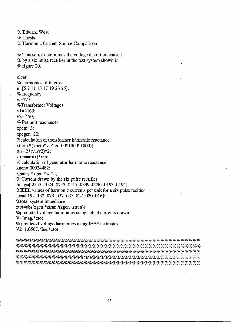
"% Edward West"% Thesis"% Harmonic Current Source Comparison
"% This script determines the voltage distortion caused"% by a six pulse rectifier in the test system shown in"% figure 20.
clear% harmonics of interestn=[5 7 11 13 17 19 23 25];% frequencyw=377;%Transformer Voltagesvi=4160;v2=.450;% Per unit reactancesxpctn=3;xpcgen=20;%calculation of transformer harmonic reactancextn=n.*(xpctn*vlA2/(100*1000*1000));rtn=.2*(vl/v2)A2;ztran=rtn+j *xtn;% calculation of generator harmonic reactancexgen=.00024482;zgen=j.*xgen.*w.*n;% Current drawn by the six pulse rectifierImag=[.2553.1024.0743.0517.0339.0296.0193.0194];%IEEE values of harmonic currents per unit for a six pulse recitierIee=[. 192.132.073.057.035.027.020.016];%total system impedanceztot=abs(zgen.*ztran./(zgen+ztran));%predicted voltage harmonics using actual currents drawnV=Imag.*ztot% predicted voltage harmonics using IEEE estimatesV2=1.0567.*Iee.*ztot
%%%%%%%%%%%%%%%%%%%%%%%%%%%%%%%%%%%%%%%%%%%%%%%%%%%%%%%%%%%%%%%%%%%%%%%%%%%%%%%%%%%%%%%%%%%%%%%%%%%%%%%%%%%%%%%%%%%%%%%%%%%%%%%%%%%%%%%%%%%%%%%%%%%%%%%%%%%%%%%%%%%%%%%%%%%%%%%%%%%%%%T%%%%%%%%%%%%%%%%%%%%%%%%%%%%%%%%%%%%%%%%%%%%%%%%
95

"% Edward West"% Thesis"% Calculation of short circuit current"% given per unit subtransient reactance"% bus voltage and total power available
clearlimit=[63000 63000 63000 63000 63000];Vb=input('Enter line to line system voltage ');xdpp=[.2];Pb=[40 50 60 70 80];hold onfor i= 1 :length(xdpp);
I=Pb./(.8*sqrt(3)*Vb*xdpp(i));plot(Pb,I* 1000)
endplot(Pb,limit/1000)xlabel('Installed Power (MW)')ylabel('Fault Current (kA)')hold off
%%%%%%%%%%%%%%%%%%%%%%%%%%%%%%%%%%%%%%%%%%%%%%%%%%%%%%%%%%%%%%%%%%%%%%%%%%%%%%%%%%%%%%%%%%%%%%%%%%%%%%%%%%%%%%%%%%%%%%%%%%%%%%%%%%%%%%%%%%%%%%%%%%%%%%%%%%%%%%%%%%%%%%%%%%%%%%%%%%%%%%%%
96

"% Edward West"% Thesis"% Calculation of O/P filter inductance"% based on method outlined in"% Keller A W, Yadusky W F, "Rectifier Design for"% Minimum Line Current Harmonics and Maximum Power"% Factor" IEEE Transactions on Power Electronics, Vol"% 7. No 2 April 1992
clear
% Normalization ReferencesVref=input('Enter nominal rms line to neutral source voltage ');Pref=input('Enter nominal rectifier o/p power ');Fref=60;Tref=2*pi/Fref;Iref=Pref/Vref;Zref=VrefA2/Pref;
% Inductance Calculation
Lon=. 1;Con=10;Lo=Lon*(Vref/(Iref*Fref))Co=Con*(Iref/(Vref*Fref))
97

"% Edward West"% Thesis"% Calculation of Generator Fault Current
xd=2.2;xq=2;xdp=.45;xdpp=.25;xqpp=.22;tdop=5;tdopp=.2;tqopp=.3;t=O:.OOOO1 :.25;
tdp=xdp*tdop/xd;tdpp=xdpp*tdopp/xdp;
ial =( 1/xd+( 1/Xdp- l/Xd). *exp(-t./tdp)+( l/xdpp- 1/Xdp). *ex p(-t./tdpp)). *cos(377*t)..-1 ./xdpp*exp(-t./ta);
hold
%title('Generator Fault Current')ylabel('Phase Current (pu)')xdpp=. 15;tdp=xdp*tdop/xd;tdpp=xdpp*tdopp/xdp;ial =( 1/xd+( 1/xdp- 1/xd). *exp(-t./tdp)+( 1/Xdpp- 1/xdp). *exp(-t./tdpp)). *cos(377*t)...
-1 ./xdpp*exp(-t./ta);
plot(t,-ia 1)h=legend('25% subtransient reactance',' 15% subtransient reactance')"% title('15% Subtransient Reactance')"% ylabel('Phase Current (pu)')xlabel('time (sec)')
98

Appendix B. LBES Comparison for Generator, Filter, and Voltage
Generator Current 10% Power1
M measured
0.9- simulated
0.8
0.7
0.6
O0.5
0.4
0.3
0.2-
0.1
01 5 7 11 13 17 19 23 25
harmonic number
Generator Current 10% Power1.5-
1_5 measured, " --- simulated
u I
1 i I I
SII 'I' !I I I I I
1, /
-0.5 -
-1.5 r I I II
0 0.005 0.01 0.015 0.02 0.025 0.03 0.035 0.04 0. 045 0.0ý5time(sec)
99

Generator Current 50% Power
measured0.9- simulated
0.8
0.7
0.6
0.5-
0.4-
0.3
0.2
0.1 -
05 7 11 13 17 19 23 25
harmonic number
Generator Current 50% Power1.5
-- measuredsimulated
1
0.5-
"Z 0
E
-0.5-
-1
-1 .5 I I I I I I I0 0.005 0.01 0.015 0.02 0.025 0.03 0.035 0.04 0.045 0.05
time(sec)
100

Generator Current 90% Power1 , ,
measured
0.9i simulated
0.8
0.7
0.6
0.5-
0.4
0.3
0.2
0.101eiN. mn m . . . .
5 7 11 13 17 19 23 25harmonic number
Generator Current 90% Power1.5
-- measuredSsimulated
1
0.5
-0.5
-1.5
-1.5 I I I I I I
0 0.005 0.01 0.015 0.02 0.025 0.03 0.035 0.04 0.045 0.05time(sec)
101

Line-Line Voltage 10% Power1 I , ,
measured0.9- simulated
0.8
0.7
0.6
0.5
0.4
0.3
0.2
0.1
0 an i .. in ".
1 5 7 11 13 17 19 23 25harmonic number
Line-Line Voltage 10% Power1.5
_ measured--- simulated
1
0.5-
0,5
-0.5
-1
-1.5 I I Ir0 0.005 0.01 0.015 0.02 0.025 0.03 0.035 0.04 0.045 0.05
time(sec)
102

Line-Line Voltage 50% Power1 , ,
M measured
0.9- simulated
0.8
0.7
0.6
"0.5
0.4
0.3
0.2
0.1
0 --5 7 11 13 17 19 23 25
harmonic number
Line-Line Voltage 50% Power1.5
___ measuredSsimulated
1 I 'A
I; isit I li
0.5 - t
-0.5 ,-
I I ( I
II IiI
II I /I
-1
-1.5-
0 0.005 0.0 1 0.015 0.02 0.025 0.03 0.035 0.04 0.045 0.05
103

Line-Line Voltage 90% Power1.4
measuredsimulated
1.2
1
I 0.8
0.6
0.4
0.2
0o II ii O N mn .. I g1 5 7 11 13 17 19 23 25
harmonic number
Line-Line Voltage 90% Power1.5
___ measuredSsimulated
1 ¼L
0.5-
0• ~II
-0.5
-I I
-1.5-0 0.005 0.01 0.015 0.02 0.025 0.03 0.035 0.04 0.045 0.05
time(sec)
104
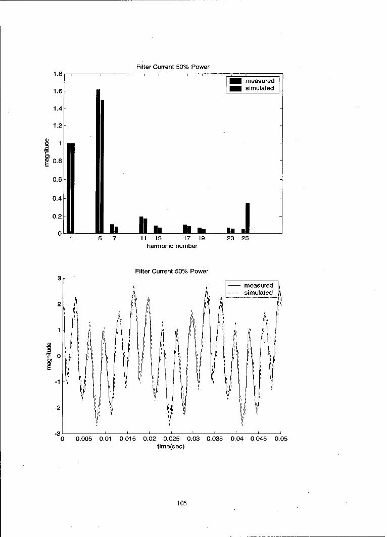
Filter Current 50% Power1.8 . .. .. .
M measured
1.6 simulated
1.4
1.2
•0.8
0.6
0.4
0.2 1
0 , I,,1 5 7 11 13 17 19 23 25
harmonic number
Filter Current 50% Power3-
measuredd2--- simulated
I i I I/
I I
I IIj I[ I III
01
0 0.805 0.01 0.015 0.02 0.025 0.03 0.035 0.04 0.045 0.05time(sec)
105

Filter Current 90% Power2
measured1.8 • simulated
1.6
1.4
1.2
0.8
0.6
0.40.hI ith mu0.20 MM Elm
1 5 7 11 13 17 19 23 25harmonic number
Filter Current 90% Power4-
measured
simulated3 -
0 0.00 0.100500, .2 .0 .3 .400500
I F
-2 I II,
time(sec)
106
1 F F

Appendix C. Tabulated Distortion Results
Table 8-2 Cruise Loading, 90 Degrees, Baseline System
Condition CruiseTemp -90Speed 0
Bus Voltage(Volts) % of Fund Gen Current (A) % of Fund Gen Current (kA) % of Fund1 436.56 100 753.28 1005 5.99 1.37209089 22.97 3.0493317 1.94 0.44438336 9.37 1.243893
11 9.73 2.22878871 15.23 2.02182513 6.23 1.42706615 8.87 1.17751717 4.31 0.98726406 3.75 0.497823.19 4.01 0.91854499 3.22 0.42746423 0.14 0.0320689 0.64 0.084962125 0.57 0.13056625 0.4 0.053101
THD 3.30 4.09 1
Condition CruiseTemp 90Speed 15
Bus Voltage(Volts) % of Fund Gen Current (A) % of Fund Gen Current (kA) % of Fund
1 426.96 100 1376.27 100
51 41.18 9.64493161 151.45 11.00438
7 7.53 1.76363125 20.28 1.473548
11 29.45 6.89760165 52.64 3.824831
13 12.44 2.91362188 19.55 1.420506
17 15.42 3.61157954 19.79 1.437945
19 10.76 2.5201424 13.14 0.95475523 13.48 3.15720442 12.95 0.94094925 9.651 2.26016489 8.61 0.625604
THD 13.54 11.92
Condition CruiseTemp 90Speed 25
Bus Voltage(Volts) % of Fund Gen Current (A) % of Fund Gen Current (kA) % of Fund
1 423.16 100 1369.92 100 3596.77 100
5 50.23 11.8702146 184.77 13.48765 539.54 15.000687 26.9 6.35693355 89.18 6.509869 264,77 7.361327
11 18.57 4.388411 39.58 2.88922 118.67 3.299349
13 11.44 2.70346914 30.91 2.256336 91.25 2.53699817 6.99 1.65185745 12.52 0.913922 37.66 1.04705119 14.26 3.36988373 8.02 0.585436 24.83 0.69034223 0.75 0.17723792 1.09 0.079567 33.91 0.9427925 0.11 0.0259949 2.11 0.154024 6.11 0.169875
THD 14.74 1 15.28 17.04
Condition CruiseTemp 90Speed 30
Bus Voltage(Volts) % of Fund Gen Current (A) % of Fund Gen Current (kA) % of Fund1 433.84 100 1334.91 100 3723.09 100
5 46.43 10.9722091 182.49 13.32122 543.65 15.114957 33.98 8.03005955 96.05 7.011358 289 8.034987
11 12.22 2.88779658 28.2 2.058514 85.44 2.375465
13 10.28 2.42934115 18.83 1.374533 57.18 1.5897617 2.48 0.58606674 1.89 0.137964 5.61 0.15597319 5.57 1.31628698 4.72 0.344546 14.61 0.40619823 6.85 1.61877304 7.72 0.563537 23.5 0.65336425 7.25 1.71329993 7.17 0.523388 21.79 0.605821
THD 13.89 15.49 16.56
107

Table 8-3 Cruise Loading, 10 Degree, Baseline SystemCondition CruiseTernP 10Speed 0
BusVoltage % of Fund Gen Current (A) % of Fund Gen Current (kA) % of Fund1 439.45 100 883.66 1005 7.06 1.60655365 28.03 3.172034497 3.16 0.71908067 12.16 1.37609488
11 8.71 1.98202298 14.16 1.6024262713 5.25 1.19467516. 7.96 0.9007989517 4.57 1.03993628 4.17 0.4719009619 3.97 0.90340198 3.39 0.3836317123 1.11 0.25258846 0.75 0.0848742725 1.43 0.32540676 0.81 0.09166421
THD 3.24 3.96
Condition CruiseTernp 10Speed 15
Bus Voltageý % of Fund Gen Current (A) % of Fund Gen Current (kA) % of Fund1 424.77 100 1506.89 1005 38.71 9.11316713 142.38 9.448599437 5.58 1.31365209 15.58 1.03391754
11 28.59 6.73070132 51.97 3.4488250613 12.39 2.91687266 19.85 1.3172826217 13.2 3.10756409 17.35 1.15137819 8.34 1.9634155 10.77 0.7147170723 12.59 2.96395696 12.48 0.8281958225 8.89 2.09289733 8.44 0.56009397
THD 12.75 10.28
Condition CruiseTemp 10Speed 25
Bus Voltage % of Fund Gen Current (A) % of Fund Gen Current (kA) 1% of Fund1 432.89 100 1374.29 100 3831.2 1005 45.22 10.4460718 184.23 13.4054676 538.26 14.0493847 30.48 7.04104969 88.11 6.41131057 261.26 6.81927333
11 17.29 3.99408626 38.49 2.80071892 114.98 3.0011484713 16.92 3.9086142 28.89 2.1021764 86.34 2.25360217 8.75 2.02129871 12.02 0.87463345 36.09 0.9420025119 5.64 1.3028714 7.9 0.57484228 23.86 0.6227813723 0.33 0.07623184 1.01 0.07349249 3.29 0.0858738825 1.67 . 0.3857793 1.59 0.1156961 4.56 0.11902276
THD 13.86 15.13 1 15.90
Condition CruiseTemp 10Speed 30
Bus Voltageý % of Fund Gen Current (A) i% of Fund Gen Current (kA) % of Fund1 431.1 100 1343.14 100 4083.56 1005 45.93 10.6100857 181.36 13.1966324 543.38 14.18302367 32.47 7.50075077 95.34 6.9374004 284.72 7.43161412
11 11.75 2.71431542 26.78 1.94864257 82.28 2.1476299913 9.74 2.24999422 18.16 1.3214096 54.38 1.4193986217 2.19 0.50590219 2.42 0.17609093 7.38 0.1926289419 5.1 1.17812839 4.66 0.33908418 13.72 0.3581123423 6.37 1.47150546 7.31 0.53191102 22.79 0.5948527925 6.42 1.48305574 6.67 0.48534152 19.59 0.51132804
THD 13.61 15.28 15.06
108

Table 8-4 Battle Loading, 90 Degree, Baseline SystemCondition BattleTernp 90Speed 0
Bus Voltage(Volts) % of Fund Gen Current (A) % of Fund Gen Current (kA) % of Fund1 430.01 100 1120.02 1005 11.39 2.64877561 45.77 4.086534
7 6.86 1.59531174 21.39 1.90978711 5.78 1.34415479 10.51 0.93837613 2.38 0.5534755 5.09 0.45445617 5.54 1.28834213 4.94 0.44106419 3.11 0.72323899 3.58 0.31963723 2.92 0.67905398 2.13 0.19017525 2.57 0.59766052 1.83 0.16339
THD 3.83 1 4.66 1 1
Condition BattleTemp 90Speed 15
Bus Voltage(Volts) % of Fund Gen Current (A) % of Fund Gen Current (kA) % of Fund
1 422.02 100 1743.29 1005 35.02 8.29818492 129.19 7.41077 2.11 0.4999763 3.74 0.214537
11 27.17 6.4380835 50.49 2.89624813 12.42 2.94298848 21.55 1.23616817 13.38 3.17046585 18.24 1.04629819 6.98 1.65395005 9.32 0.53462123 8.66 2.05203545 9.26 0.53118125 7.64 1.81034074 7.77 0.4457091
THD 11.73 8.14 1
Condition BattleTemp 90Speed 25
Bus Voltage(Volts) % of Fund Gen Current (A) % of Fund Gen Current (kA) % of Fund1 429.68 100 1425.58 100 4205.67 1005 45.96 10.6963322 190.74 13.37982 545.06 12.960122887 30.58 7.11692422 90.27 6.33216 262.62 6.244427166
11 16.46 3.83075777 37.56 2.634717 110.47 2.62669206113 15.41 3.58638987 27.92 1.958501 79.16 1.88222090717 7.49 1.7431577 10.39 0.728826 30.56 0.72663808619 4.33 1.00772668 6.34 0.444731 18.89 ,0.44915554523 1.03 0.23971327 2.19 0.153622 6.57 0.15621767825 1.68 0.39098864 2.17 0.152219 6.51 0.154791032
]HD 13.89 15.02 14.611
Condition BattleTemp 90Speed 30
Bus Voltage(Volts) % of Fund Gen Current (A) % of Fund Gen Current (kA) % of Fund1 427.95 100 1430.28 100 3972.9 1005 45.83 10.6660771 185.86 13.0375 553.42 13.158902157 31.94 7.43343884 95.05 6.667462 285.9 6.797965604
11 11.15 2.59495438 27.34 1.917816 82.6 1.96401524613 8.77 2.04105381 16.46 1.154618 49.98 1.18839566617 2.28 0.53062744 2.75 0.192904 8.36 0.19877926719 5.14 1.19623906 5.45 0.382301 16.52 0.39280304923 6.22 1.4475889 8.28 0.580816 25.11 0.59705112425 5.88 1.36846025 6.56 0.460164 19.98 0.475072937
THD 13.55 14.63 15.70
109

Table 8-5 Battle Loading, 10 Degrees, Baseline SystemCondition BattleTIemp 90Speed 0
Bus Voltage(Volts) %of Fund Gen Current (A) % of Fund Gen Current (kA) % of Fund1 436.25i 100 805.93 1005 7.34 1.682521 28.99 3.597087
7 3.29 0.754155 12.48 1.54852211 9.2 2.108883 14.76 1.83142513 5.57 1.276791 8.25 1.02366217i 4.97 1.139255 4.56 0.56580619 4.38 1.004011 3.73 0.46281923 1.25 0.286533 0.88 0.10919125 1.67 0.3828081 0.96 0.119117
THID 1 _3.461_1 4.50
Condition BattleTemp 90Speed 15
_....... Bus Volta e Volts 7 % of Fund Gen Current (A) % of Fund Gen Current (kA) % of Fund
1 426.54 100 1426.47 1005 39.94 9.363717 145.61 10.207727 5.92 1.387912 15.78 1.106227
11 30.18 7.075538 53.66 3.76173413 13.04 3.057158 20.09 1.40837217 14.52 3.404136 18.47 1.294805 1 119 9.35 2.192057 11.53 0.80828923 13.99 3.27988 13.18 0.92395925 10.09 2.365546 9.08 0.6365361
TH 1 13.36 11.12 1 _1
Condition "BattleTIemp 90Speed 25
_........ Bus Voltage(Volts) %of Fund Gen Current (A) % of Fund Gen Current (kA) % of Fund1 435.14 100 1376.41 100 3684.71 1005 45.98 10.56671 185.86 13.50324 542.87 14.733057 30.93 7.108057 89.21 6.481354 264.75 7.185097
11 17.77 4.083743 38.64 2.807303 115.81 3.14298813 17.55 4.033185 29.36 2.133085 88.19 2.39340417 8.81 2.024636 11.89 0.863841 35.74 0.96995419 5.79 1.330606 7.92 0.57541 23.82 0.64645523 0.18 0.041366 1.17 0.085004 3.59 0.09743125 0.24 0.055155 1.71 0.124236 5.21 0.141395
THD 14.04 15.24 16.67
Condition BattleTem p 90speed 30
IIIIIII . Bus Voltage(Volts) % of Fund Gen Current A) % of Fund Gen Current (kA) % of Fund1 433.42 100 1416.16 100 3668.44 1005 46.36 10.65404 183.86 13.35794 547.19 14.850297 32.89 7.558487 95.19 6.915817 286.15 7.765876
11 11.86 2.72556 27.85 2.02338 84.33 2.28864713 10.06 2.3119 17.81 1.293946 54.13 1.46904417 2.24 0.514777 23.23 1.687724 7.01 0.19024619 5.32 1.222595 5.13 0.372709 15.43 0.41875823 6.16 1.415636 8.08 0.587034 24.45 0.66355325 6.66 1.530542 6.65 0.483141 20.23 0.549026
THD 13.69 14.76 16.84
110

Table 8-6 Anchor Loading, Baseline System
Condition AnchorTemp 90Speed 0
.Bus Voltage(Volts) % of Fund Gen Current (A) % of Fund Gen Current (kA) % of Fund1 442.88 100 835.95 1005 7.35 1.659592 27.83 3.329146487 3.61 0.815119 10.42 1.246486034
11 10.16 2.294075 16.67 1.99413840513 5.34 1.205744 7.9 0.94503259817 2.89 0.652547 2.75 0.32896704319 2.82 0.636741 2.57 0.30743465523 1.95 0.4403 1.78 0.21293139525 1.43 0.322887 1.39 0.1662778871
THD 3.35 4.21 1
Condition AnchorTemp 10Speed 0
Speed Bus Voltage(Volts) % of Fund Gen Current (A) % of Fund Gen Current (kA) % of Fund1 439.98 100 843.69 1005 7.59 1.725078 28.59 3.3886854187 3.53 0.802309 10.34 1.225568633
11 10.01 2.275103 16.63 1.9711031313 5.31 1.206873 7.82 0.92688072617 2.86 0.65003 2.76 0.32713437419 2.85 0.647757 2.58 0.30579952423 1.88 0.427292 1.73 0.20505161825 1.35 0.306832 1.28 0.151714492
THD 3.37 1 4.24 1
111
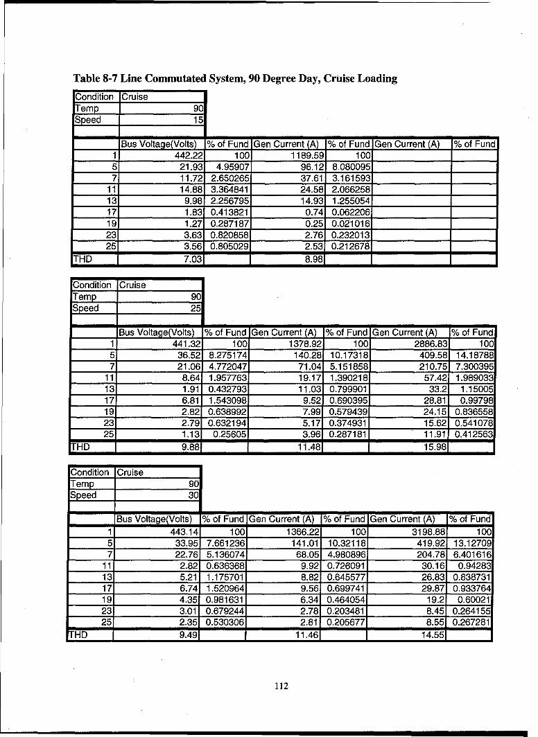
Table 8-7 Line Commutated System, 90 Degree Day, Cruise LoadingCondition CruiseTemnp 90Speed 115
Bus Voltage(Volts) % of Fund Gen Current (A) % of Fund Gen Current (A) % of Fund1 442.22 100 1189.59 1005 21.93 4.95907 96.12 8.0800957 11.72 2.650265 37.61 3.161593
11 14.88 3.364841 24.58 2.06625813 9.98 2.256795 14.93 1.25505417 1.83 0.413821 0.74 0.06220619 1.27 0.287187 0.25 0.02101623 3.63 0.820858 2.76 0.23201325 3.56 0.805029 2.53 0.212678
THD 7.03 8.98 1 1 1
Condition CruiseTemnp 90Speed 25
-0 Bus Voltage(Volts) % of Fund Gen Current (A) % of Fund Gen Current (A) % of Fund1 441.32 100 1378.92 100 2886.83 1005 36.52 8.275174 140.28 10.17318 409.58 14.187887 21.06 4.772047 71.04 5.151858 210.75 7.300395
11 8.64 1.957763 19.17 1.390218 57.42 1.98903313 1.91 0.432793 11.03 0.799901 33.2 1.1500517 6.81 1.543098 9.52 0.690395 28.81 0.9979819 2.82 0.638992 7.99 0.579439 24.15 0.83655823 2.79 0.632194 5.17 0.374931 15.62 0.54107825 1.13 0.25605 3.96 0.287181 11.91 0.412563-I
THD 9.88 11.48 15.98
Condition Cruise"lemp 9(0Speed 30
Bus Voltage(Volts) % of Fund Gen Current (A) % of Fund Gen Current (A) % of Fund1 443.14 100 1366.22 100 3198.88 1005 33.95 7.661236 141.01 10.32118 419.92 13.127097 22.76 5.136074 68.05 4.980896 204.78 6.401616
11 2.82 0.636368 9.92 0.726091 30.16 0.9428313 5.21 1.175701 8.82 0.645577 26.83 0.83873117 6.74 1.520964 9.56 0.699741 29.87 0.93376419 4.35 0.981631 6.34 0.464054 19.2 0.6002123 3.01 0.679244 2.78 0.203481 8.45 0.26415525 2.35 0.530306 2.81 0.205677 8.55 0.267281
THD 9.49 1 11.46 1 14.551
112

Table 8-8 Filter System Tabulated Results
Condition CruiseTernp 90Speed 15
,Bus Voltage(Volts) % of Fund Gen Current (A) % of Fund Gen Current (A) % of Fund
1 435.97 100 1283.73 1005 2.52 0.578021 1.29 0.1004887 2.49 0.57114 5.53 0.430776
11 18.22 4.179187 31.85 2.48105113 6.88 1.57809 10.7 0.83350917 8.67 1.988669 11.6 0.90361719 2.6 0.596371 4.09 0.31860323 8.2 -1.880863 8.56 0.666807,25 6 1.376241 5.55 0.4323341
THD 5.50 2.93 1
Condition CruiseTemp 90Speed 25
Bus Voltage(Volts) % of Fund Gen Current (A) % of Fund Gen Current (A) % of Fund1 436 100 1378.92 100 2886.83 1005 5.98 1.37156 140.28 10.17318 409.58 14.187887 20.12 4.614679 71.04 5.151858 210.75 7.300395
11 17.29 3.965596 19.17 1.390218 57.42 1.98903313 26.47 6.071101 11.03 0.799901 33.2 1.1500517 11.25 2.580275 9.52 0.690395 28.81 0.9979819 9.07 2.080275 7.99 0.579439 24.15 0.83655823 6.56 1.504587 5.17 0.374931 15.62 0.54107825 4.88 1.119266 3.96 0.287181 11.91 0.412563
THD 9.46 11.48 15.98
Condition CruiseTemp 90Speed 30
Bus Voltage(Volts) % of Fund Gen Current (A) % of Fund Gen Current (A) % of Fund1 432.14 100 1366.22 100 3198.88 1005 5.99 1.386125 141.01 10.32118 419.92 13.127097 28.45 6.583515 68.05 4.980896 204.78 6.401616
11 14.56 3.369278 9.92 0.726091 30.16 0.9428313 11.25 2.603323 8.82 0.645577 26.83 0.83873117 14.37 3.325311 9.56 0.699741 29.87 0.93376419 3.21 0.742815 6.34 0.464054 19.2 0.6002123 5.22 1.207942 2.78 0.203481 8.45 0.26415525 5.9 1.365298 2.81 0.205677 8.55 0.267281
THD 8.82 11.46 1 14.55
113

Table 8-9 12 Pulse System Tabulated Results
Condition CruiseTemp 90Speed 15
-Bus Voltage(Volts) % of Fund Gen Current (A) % of Fund Gen Current (A) % of Fund
1 443.98 100 1254.38 1005 5.47 1.232037 22.45 1.7897297 1.55 0.349115 8.95 0.7135
11 19.54 4.401099 32.98 2.62918713 13.64 3.07221 19.98 1.59281917 4.02 0.905446 3.93 0.31330219 4.22 0.950493 3.64 0.29018323 4.66 1.049597 5.17 0.41215625 4.42 0.99554 4.36 0.347582
THD 5.84 3.69
Condition CruiseTemp 90
Speed 25
Bus Voltage(Volts) % of Fund Gen Current (A) % of Fund Gen Current (A) % of Fund1 429.4 100 1019.66 100 3734.27 1005 3.97 0.924546 13.24 1.298472 25.53 0.6836687 0.4 0.093153 5.58 0.547241 7.08 0.189595
11 26.2 6.101537 44.03 4.318106 137.67 3.68666413 20.45 4.762459 30.39 2.980405 92.63 2.48053817 2.07 0.482068 2.67 0.261852 4.15 0.11113319 2.52 0.586865 2.55 0.250083 3.96 0.10604523 4.18 0.973451 3.37 0.330502 12.24 0.32777525 4.15 0.966465 4.12 0.404056 11.04 0.29564
THD 7.93 1 5.46 4.52
Condition CruiseTemp 90Speed 30
Bus Voltale(Volts) .% of Fund Gen Current (A) % of Fund Gen Current (A) % of Fund
1 440.87 100 1302.76 100 3515.63 1005 3.38 0.766666 8.04 0.617151 19.87 0.565197 0.78 0.176923 2.8 0.214928 5.77 0.164124
11 24.75 5.6139 42.36 3.251558 13.02 0.37034613 17.26 3.914986 26.75 2.053333 78.87 2.2434117 1.96 0.444575 1.69 0.129725 2.97 0.0844819 2.25 0.510355 0.53 0.040683 3.52 0.10012423 8.23 1.866763 8.94 0.686235 2.57 0.07310225 7.65 1.735205 6.88 0.52811 2.22 0.063147-I
THD 7.36 3.99 2.35[M
114