4. categorical data analysis 2014 - umass amherstcourses.umass.edu/biep640w/pdf/4. categorical data...
TRANSCRIPT

PubHlth 640 - Spring 2014 4. Categorical Data Analysis Page 1 of 85
Unit 4
Categorical Data Analysis
“Don’t ask what it means, but rather how it is used”
- L. Wittgenstein
Is frequency of exercise associated with better health? Is the proportion of adults who visit their doctor more than once a year, significantly lower among the frequent exercisers than among the non-exercisers? Is alcohol associated with higher risk of lung cancer? Is the apparent association a fluke because we have failed to account for the relationship between drinking and smoking? Is greater exposure to asbestos associated with the development pleural plaques? Is more exposure associated with more pleural plaques? Units 3 (Discrete Distributions) and 4 (Categorical Data Analysis) pertain to questions such as these and are an introduction to the analysis of count data that can be represented in a contingency table (a two-way cross-tabulation of the counts of individuals with each profile of traits; eg non-drinker and lung cancer). Data that are counts are categorical data. A categorical variable is measured on a scale that is nominal (eg – religion) or ordinal (eg – diagnosis coded as “benign”, “suspicious”, or “malignant”). An example of a two-way cross-tabulation of categorical data is a cross-tabulation of frequency of visits to the doctor (1=less than every five years, 2=annually, and 3=every six months) by diagnosis, coded as above. A categorical data analysis of these data might explore the nature and significance, if any, of the association between the two variables. Thus, there are many uses for categorical data analyses, especially in epidemiology and public health Unit 4 (Categorical Data Analysis) is an introduction to some basic methods for the analysis of categorical data: (1) association in a 2x2 table; (2) variation of a 2x2 table association, depending on the level of another variable; and (3) trend in outcome in a contingency table. Tip - These methods require minimal assumptions for their validity and, in particular, do not assume a regression model. These methods, in contrast to regression approaches, have the added advantage of giving us a much closer look at the data than is generally afforded by regression techniques. Tip – always precede a logistic regression analysis with contingency table analyses.
PubHlth 640 - Spring 2014 4. Categorical Data Analysis Page 2 of 85
Table of Contents
Topics
1. Learning Objectives ……………………………………………………
2. Examples of Categorical Data ………..……………….………………
3. Hypotheses of Independence, No Association, Homogeneity .…………
4. The Chi Square Test of No Association in an RxC Table ……….……...
5. Rejection of Independence: The Chi Square Residual………………….
6. Confidence Interval Estimation of RR and OR ………………………...
7. Strategies for Controlling Confounding ……………………………..….
8. Multiple 2x2 Tables - Stratified Analysis of Rates ……………………
A. Woolf Test of Homogeneity of Odds Ratios………………..……………… B. Breslow-Day-Tarone Test of Homogeneity of Odds Ratios ……………… C. Mantel Haenszel Test of No Association ………………………………….
9. The R x C Table – Test for (Linear) Trend …………………………….
10. Factors Associated with Mammography Screening …………………….
11. The Chi Square Goodness-of-Fit Test …………….……………………
3
4
9
10
16
20
24
26
31 33 37
40
46
52
Appendices A. The Chi Square Distribution …………………………………………… B. Probability Models for the 2x2 Table …………………………………… C. Concepts of Observed and Expected …………………………………… D. Review: Measures of Association in a 2x2 Table ……………………… E. Review: Confounding of Rates …………………………………………
62 66 68 72 78
PubHlth 640 - Spring 2014 4. Categorical Data Analysis Page 3 of 85
Learning Objectives
When you have finished this unit, you should be able to:
§ Perform and interpret the chi square test of association in a single 2x2 table.
§ Define and distinguish between exposure-outcome associations that are confounded versus effect modified.
§ Perform and interpret an analysis of stratified 2x2 tables, using Mantel-Haenszel methods.
§ Perform and interpret the test of trend for RxC tables of counts of ordinal data that are suitable for explorations of dose-response
§ Perform and interpret a chi square goodness-of-fit (GOF) test
Note - Currently, this unit does not discuss matched pairs or matched data.
PubHlth 640 - Spring 2014 4. Categorical Data Analysis Page 4 of 85
2. Examples of Categorical Data
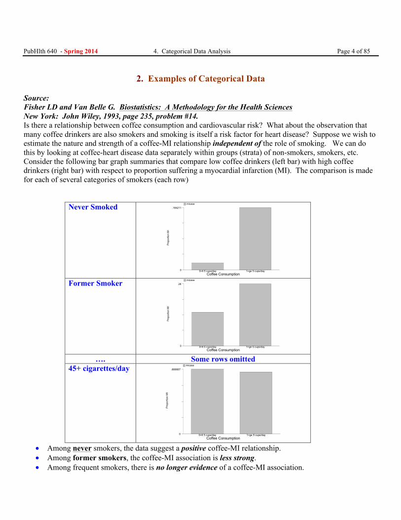
Source: Fisher LD and Van Belle G. Biostatistics: A Methodology for the Health Sciences New York: John Wiley, 1993, page 235, problem #14. Is there a relationship between coffee consumption and cardiovascular risk? What about the observation that many coffee drinkers are also smokers and smoking is itself a risk factor for heart disease? Suppose we wish to estimate the nature and strength of a coffee-MI relationship independent of the role of smoking. We can do this by looking at coffee-heart disease data separately within groups (strata) of non-smokers, smokers, etc. Consider the following bar graph summaries that compare low coffee drinkers (left bar) with high coffee drinkers (right bar) with respect to proportion suffering a myocardial infarction (MI). The comparison is made for each of several categories of smokers (each row)
Never Smoked
Pro
porti
on M
I
Coffee Consumption0
.184211 micase
0=lt 5 cups/day 1=ge 5 cups/day
Former Smoker
Prop
ortio
n M
I
Coffee Consumption0
.28 micase
0=lt 5 cups/day 1=ge 5 cups/day
…. Some rows omitted
45+ cigarettes/day
Pro
porti
on M
I
Coffee Consumption0
.666667 micase
0=lt 5 cups/day 1=ge 5 cups/day
• Among never smokers, the data suggest a positive coffee-MI relationship. • Among former smokers, the coffee-MI association is less strong. • Among frequent smokers, there is no longer evidence of a coffee-MI association.
PubHlth 640 - Spring 2014 4. Categorical Data Analysis Page 5 of 85
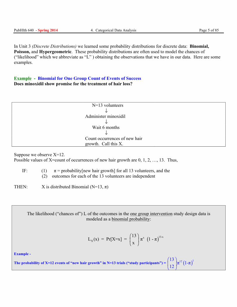
In Unit 3 (Discrete Distributions) we learned some probability distributions for discrete data: Binomial, Poisson, and Hypergeometric. These probability distributions are often used to model the chances of (“likelihood” which we abbreviate as “L” ) obtaining the observations that we have in our data. Here are some examples. Example - Binomial for One Group Count of Events of Success Does minoxidil show promise for the treatment of hair loss? N=13 volunteers
↓
Administer minoxidil ↓
Wait 6 months ↓
Count occurrences of new hair growth. Call this X.
Suppose we observe X=12. Possible values of X=count of occurrences of new hair growth are 0, 1, 2, …, 13. Thus, IF: (1) π = probability[new hair growth] for all 13 volunteers, and the
(2) outcomes for each of the 13 volunteers are independent THEN: X is distributed Binomial (N=13, π)
The likelihood (“chances of”) L of the outcomes in the one group intervention study design data is
modeled as a binomial probability:
( )13-xxX
13L (x) = Pr[X=x] = π 1 - π
x⎛ ⎞⎜ ⎟⎝ ⎠
Example -
The probability of X=12 events of “new hair growth” in N=13 trials (“study participants”) = ( )11213π 1-π
12⎛ ⎞⎜ ⎟⎝ ⎠

PubHlth 640 - Spring 2014 4. Categorical Data Analysis Page 6 of 85 Example - The Product of 2 Binomials is used for the 2 Independent Counts in a Cohort Trial In a randomized controlled trial, is minoxidil better than standard care for the treatment of hair loss? Consent of N=30 volunteers
↓ Randomization
Standard Care N1 = 17
Minoxidil N2 = 13
Administer standard care ↓
Administer minoxidil ↓
Wait 6 months ↓
Wait 6 months ↓
Count occurrences of new hair growth. Call this X1.
Count occurrences of new hair growth. Call this X2.
This design produces a 2x2 table array of count data that is correctly modeled using the product of two binomial distributions. New Growth Not
Minoxidil
X2 = 12 N2 = 13
Standard care
X1 = 6 N1 = 17
IF: (1) π1 = probability[new hair growth] on standard care (2) π2 = probability[new hair growth] on minoxidil (3) The outcomes for all 30 trial participants are independent THEN: (1) X1 is distributed Binomial (N1 =17, π1) (2) X2 is distributed Binomial (N2 =13, π2)
The likelihood (“chances of”) L of the outcomes in the two group cohort study design data is
modeled as the product of 2 binomial probabilities:
( ) ( )1 21 2
1 2
17-x 13-xx xX 1 2 1 1 2 2 1 1 2 2
1 2
17 13L (x ,x ) = Pr[X =x and X =x ] = π 1 - π * π 1 - π
x xX
⎧ ⎫ ⎧ ⎫⎛ ⎞ ⎛ ⎞⎪ ⎪ ⎪ ⎪⎨ ⎬ ⎨ ⎬⎜ ⎟ ⎜ ⎟⎪ ⎪ ⎪ ⎪⎝ ⎠ ⎝ ⎠⎩ ⎭ ⎩ ⎭
Example -
The probability of X1=6 and X2=13 events in the standard and minoxidil groups is = ( ) ( )11 16 121 1 2 2
17 13π 1-π * π 1-π
6 12⎛ ⎞ ⎛ ⎞⎜ ⎟ ⎜ ⎟⎝ ⎠ ⎝ ⎠

PubHlth 640 - Spring 2014 4. Categorical Data Analysis Page 7 of 85
Example - The Product of 2 Binomials is used for the 2 History Counts in a Case-Control Study Is history of oral contraceptive (OC) use associated with thrombo-embolism? Enroll cases of thromboembolism N1 = 100
Enroll controls: w/o thromboembolism N2 = 200
Query history of OC use ↓
Query history of OC use ↓
↓
↓
Count histories of OC use. Call this X1.
Count histories of OC use. Call this X2.
This design also produces a 2x2 table array of count data that is correctly modeled using two binomial distributions. Case Control
History of OC Use
X1 = 65
X2 = 118
Not N1 = 100 N2 = 200
Reminder: A case-control design does not permit the estimation of probabilities of disease. IF: (1) π1 = probability[history of OC use] among cases (2) π2 = probability[history of OC use] among controls (3) The histories for all 300 observations are independent THEN: (1) X1 is distributed Binomial (N=100, π1) (2) X2 is distributed Binomial (N=200, π2)
The likelihood (“chances of”) L of the outcomes in the two group case-control study design data is
modeled as the product of 2 binomial probabilities:
( ) ( )1 21 2
1 2
100-x 200-xx xX 1 2 1 1 2 2 1 1 2 2
1 2
100 200L (x ,x ) = Pr[X =x and X =x ] = π 1 - π * π 1 - π
x xX
⎧ ⎫ ⎧ ⎫⎛ ⎞ ⎛ ⎞⎪ ⎪ ⎪ ⎪⎨ ⎬ ⎨ ⎬⎜ ⎟ ⎜ ⎟⎪ ⎪ ⎪ ⎪⎝ ⎠ ⎝ ⎠⎩ ⎭ ⎩ ⎭
Example
The probability of X1=65 and X2=118 counts of OC use history is = ( ) ( )35 8265 1181 1 2 2
100 200π 1-π * π 1-π
65 118⎛ ⎞ ⎛ ⎞⎜ ⎟ ⎜ ⎟⎝ ⎠ ⎝ ⎠
PubHlth 640 - Spring 2014 4. Categorical Data Analysis Page 8 of 85
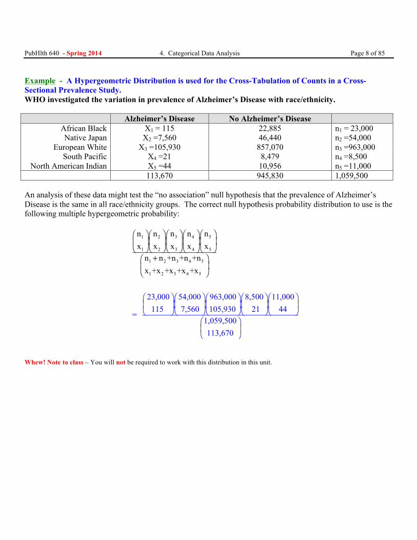
Example - A Hypergeometric Distribution is used for the Cross-Tabulation of Counts in a Cross-Sectional Prevalence Study. WHO investigated the variation in prevalence of Alzheimer’s Disease with race/ethnicity. Alzheimer’s Disease No Alzheimer’s Disease
African Black X1 = 115 22,885 n1 = 23,000 Native Japan X2 =7,560 46,440 n2 =54,000
European White X3 =105,930 857,070 n3 =963,000 South Pacific X4 =21 8,479 n4 =8,500
North American Indian X5 =44 10,956 n5 =11,000 113,670 945,830 1,059,500
An analysis of these data might test the “no association” null hypothesis that the prevalence of Alzheimer’s Disease is the same in all race/ethnicity groups. The correct null hypothesis probability distribution to use is the following multiple hypergeometric probability:
3 51 2 4
1 2 3 4 5
1 2 3 4 5
1 2 3 4 5
n nn n nx x x x x
n n +n +n +nx +x +x +
23,000 54,000 963,000 8,500 11,000 115 7,560 105,930 21 44
= 1,059,500 113,670
x +x
⎛ ⎞⎛ ⎞⎛ ⎞⎛ ⎞⎛ ⎞⎜ ⎟⎜ ⎟⎜ ⎟⎜ ⎟⎜ ⎟⎝
⎛ ⎞ ⎛ ⎞⎛ ⎞⎛ ⎞ ⎛ ⎞⎜ ⎟ ⎜ ⎟⎜ ⎟⎜ ⎟ ⎜ ⎟
⎝ ⎠⎝ ⎠ ⎝ ⎠⎝ ⎠ ⎝ ⎠+⎛ ⎞
⎜ ⎟⎝ ⎠
⎠⎝ ⎠⎝ ⎠⎝ ⎠⎝ ⎠⎛ ⎞⎜ ⎟⎝ ⎠
Whew! Note to class – You will not be required to work with this distribution in this unit.
PubHlth 640 - Spring 2014 4. Categorical Data Analysis Page 9 of 85
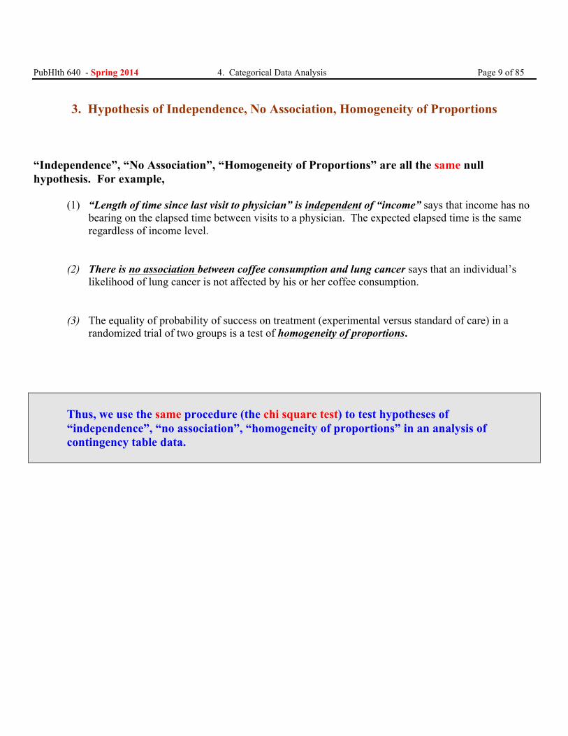
3. Hypothesis of Independence, No Association, Homogeneity of Proportions
“Independence”, “No Association”, “Homogeneity of Proportions” are all the same null hypothesis. For example,
(1) “Length of time since last visit to physician” is independent of “income” says that income has no bearing on the elapsed time between visits to a physician. The expected elapsed time is the same regardless of income level.
(2) There is no association between coffee consumption and lung cancer says that an individual’s likelihood of lung cancer is not affected by his or her coffee consumption.
(3) The equality of probability of success on treatment (experimental versus standard of care) in a randomized trial of two groups is a test of homogeneity of proportions.
Thus, we use the same procedure (the chi square test) to test hypotheses of “independence”, “no association”, “homogeneity of proportions” in an analysis of contingency table data.
PubHlth 640 - Spring 2014 4. Categorical Data Analysis Page 10 of 85
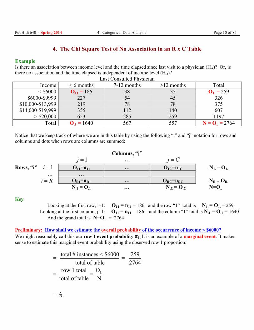
4. The Chi Square Test of No Association in an R x C Table Example Is there an association between income level and the time elapsed since last visit to a physician (HA)? Or, is there no association and the time elapsed is independent of income level (HO)?
Last Consulted Physician Income < 6 months 7-12 months >12 months Total
< $6000 O11 = 186 38 35 O1. = 259 $6000-$9999 227 54 45 326
$10,000-$13,999 219 78 78 375 $14,000-$19,999 355 112 140 607
> $20,000 653 285 259 1197 Total O.1 = 1640 567 557 N = O.. = 2764
Notice that we keep track of where we are in this table by using the following “i” and “j” notation for rows and columns and dots when rows are columns are summed: Columns, “j” j =1 … j C= Rows, “i” i = 1 O11=n11 … O1C=n1C N1. = O1. … … i R= OR1=nR1 … ORC=nRC NR. = OR.
N.1 = O.1 … N.C = O.C N=O.. Key Looking at the first row, i=1: O11 = n11 = 186 and the row “1” total is N1. = O1. = 259 Looking at the first column, j=1: O11 = n11 = 186 and the column “1” total is N.1 = O.1 = 1640 And the grand total is N=O.. = 2764 Preliminary: How shall we estimate the overall probability of the occurrence of income < $6000? We might reasonably call this our row 1 event probability π1. It is an example of a marginal event. It makes sense to estimate this marginal event probability using the observed row 1 proportion:
1.
1.
total # instances < $6000 259= = total of table 2764
row 1 total O= = total of table N
ˆ= π
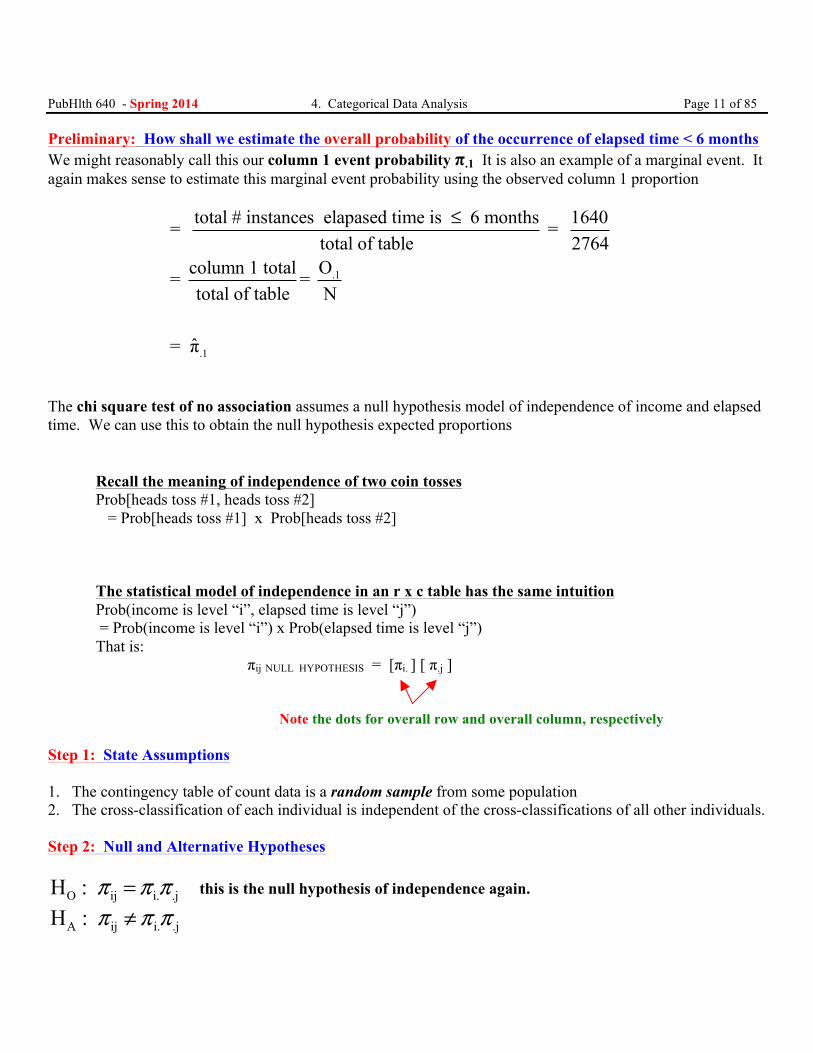
PubHlth 640 - Spring 2014 4. Categorical Data Analysis Page 11 of 85 Preliminary: How shall we estimate the overall probability of the occurrence of elapsed time < 6 months We might reasonably call this our column 1 event probability π.1 It is also an example of a marginal event. It again makes sense to estimate this marginal event probability using the observed column 1 proportion
.1
.1
total # instances elapased time is 6 months 1640= = total of table 2764
column 1 total O= = total of table N
ˆ= π
≤
The chi square test of no association assumes a null hypothesis model of independence of income and elapsed time. We can use this to obtain the null hypothesis expected proportions
Recall the meaning of independence of two coin tosses Prob[heads toss #1, heads toss #2] = Prob[heads toss #1] x Prob[heads toss #2] The statistical model of independence in an r x c table has the same intuition
Prob(income is level “i”, elapsed time is level “j”) = Prob(income is level “i”) x Prob(elapsed time is level “j”) That is: πij NULL HYPOTHESIS = [πi. ] [ π.j ] Note the dots for overall row and overall column, respectively Step 1: State Assumptions 1. The contingency table of count data is a random sample from some population 2. The cross-classification of each individual is independent of the cross-classifications of all other individuals. Step 2: Null and Alternative Hypotheses
O ij i. .jH : π π π= this is the null hypothesis of independence again.
A ij i. .jH : π π π≠
PubHlth 640 - Spring 2014 4. Categorical Data Analysis Page 12 of 85
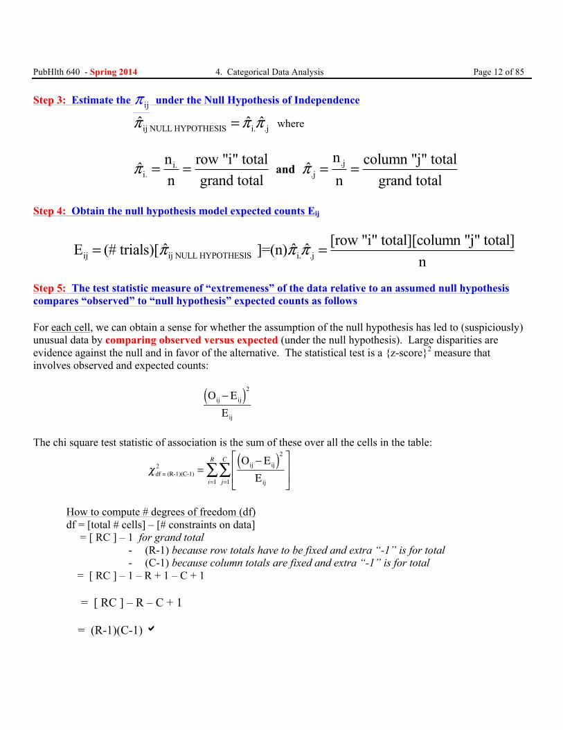
Step 3: Estimate the ijπ under the Null Hypothesis of Independence
ij NULL HYPOTHESIS i. .jˆ ˆ ˆπ π π= where
i.i.
n row "i" totalˆn grand total
π = = and .j.j
n column "j" totalˆn grand total
π = =
Step 4: Obtain the null hypothesis model expected counts Eij
ij ij NULL HYPOTHESIS i. .j[row "i" total][column "j" total]ˆ ˆ ˆE (# trials)[ ]=(n)
nπ π π= =
Step 5: The test statistic measure of “extremeness” of the data relative to an assumed null hypothesis compares “observed” to “null hypothesis” expected counts as follows For each cell, we can obtain a sense for whether the assumption of the null hypothesis has led to (suspiciously) unusual data by comparing observed versus expected (under the null hypothesis). Large disparities are evidence against the null and in favor of the alternative. The statistical test is a {z-score}2 measure that involves observed and expected counts:
Oij − Eij( )2Eij
The chi square test statistic of association is the sum of these over all the cells in the table:
χdf = (R-1)(C-1)2 =
Oij − Eij( )2
Eij
⎡
⎣⎢⎢
⎤
⎦⎥⎥j=1
C
∑i=1
R
∑
How to compute # degrees of freedom (df) df = [total # cells] – [# constraints on data] = [ RC ] – 1 for grand total
- (R-1) because row totals have to be fixed and extra “-1” is for total - (C-1) because column totals are fixed and extra “-1” is for total
= [ RC ] – 1 – R + 1 – C + 1 = [ RC ] – R – C + 1 = (R-1)(C-1) a
PubHlth 640 - Spring 2014 4. Categorical Data Analysis Page 13 of 85
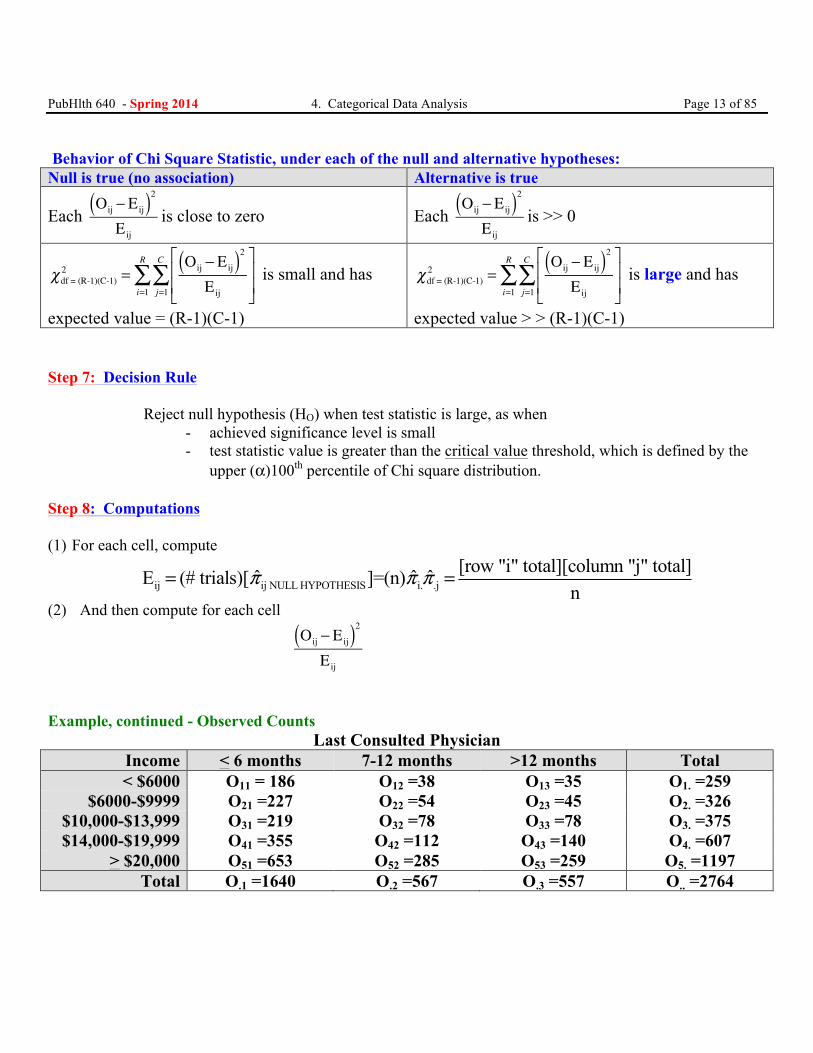
Behavior of Chi Square Statistic, under each of the null and alternative hypotheses: Null is true (no association) Alternative is true
Each Oij − Eij( )2Eij
is close to zero Each Oij − Eij( )2Eij
is >> 0
χdf = (R-1)(C-1)2 =
Oij − Eij( )2
Eij
⎡
⎣⎢⎢
⎤
⎦⎥⎥j=1
C
∑i=1
R
∑ is small and has
expected value = (R-1)(C-1)
χdf = (R-1)(C-1)2 =
Oij − Eij( )2
Eij
⎡
⎣⎢⎢
⎤
⎦⎥⎥j=1
C
∑i=1
R
∑ is large and has
expected value > > (R-1)(C-1)
Step 7: Decision Rule Reject null hypothesis (HO) when test statistic is large, as when
- achieved significance level is small - test statistic value is greater than the critical value threshold, which is defined by the
upper (α)100th percentile of Chi square distribution. Step 8: Computations (1) For each cell, compute
ij ij NULL HYPOTHESIS i. .j[row "i" total][column "j" total]ˆ ˆ ˆE (# trials)[ ]=(n)
nπ π π= =
(2) And then compute for each cell
Oij − Eij( )2Eij
Example, continued - Observed Counts
Last Consulted Physician Income < 6 months 7-12 months >12 months Total < $6000 O11 = 186 O12 =38 O13 =35 O1. =259
$6000-$9999 O21 =227 O22 =54 O23 =45 O2. =326 $10,000-$13,999 O31 =219 O32 =78 O33 =78 O3. =375 $14,000-$19,999 O41 =355 O42 =112 O43 =140 O4. =607
> $20,000 O51 =653 O52 =285 O53 =259 O5. =1197 Total O.1 =1640 O.2 =567 O.3 =557 O.. =2764
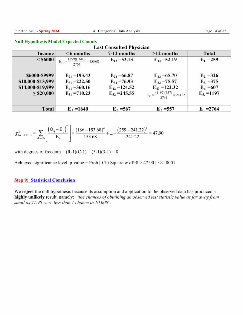
PubHlth 640 - Spring 2014 4. Categorical Data Analysis Page 14 of 85 Null Hypothesis Model Expected Counts
Last Consulted Physician Income < 6 months 7-12 months >12 months Total < $6000 E11 = =( )( ) .259 1640
276415368
E12 =53.13 E13 =52.19 E1. =259
$6000-$9999 E21 =193.43 E22 =66.87 E23 =65.70 E2. =326 $10,000-$13,999 E31 =222.50 E32 =76.93 E33 =75.57 E3. =375 $14,000-$19,999 E41 =360.16 E42 =124.52 E43 =122.32 E4. =607
> $20,000 E51 =710.23 E52 =245.55 E53 = =( )( ) .1197 5572764
24122
E5. =1197
Total E.1 =1640 E.2 =567 E.3 =557 E.. =2764
χ(R−1)(C−1)2 =
Oij − Eij( )2
Eij
⎡
⎣⎢⎢
⎤
⎦⎥⎥all cells
∑ =186 −153.68( )2
153.68+ ...+ 259 − 241.22( )2
241.22= 47.90
with degrees of freedom = (R-1)(C-1) = (5-1)(3-1) = 8 Achieved significance level, p-value = Prob [ Chi Square w df=8 > 47.90] << .0001 Step 9: Statistical Conclusion We reject the null hypothesis because its assumption and application to the observed data has produced a highly unlikely result, namely: “the chances of obtaining an observed test statistic value as far away from small as 47.90 were less than 1 chance in 10,000”.
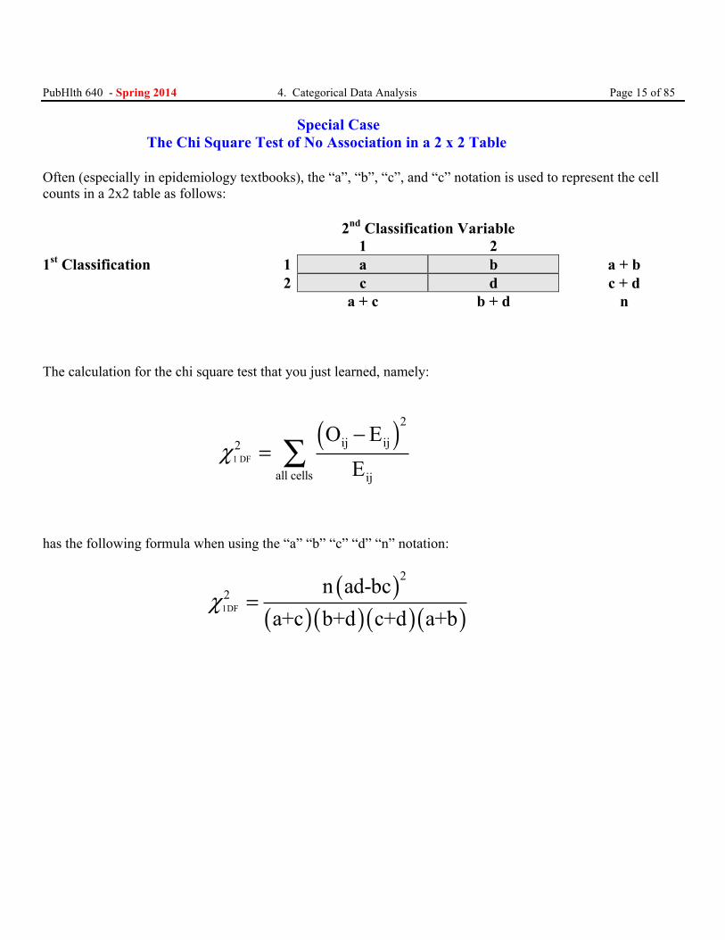
PubHlth 640 - Spring 2014 4. Categorical Data Analysis Page 15 of 85 Special Case The Chi Square Test of No Association in a 2 x 2 Table Often (especially in epidemiology textbooks), the “a”, “b”, “c”, and “c” notation is used to represent the cell counts in a 2x2 table as follows: 2nd Classification Variable 1 2 1st Classification 1 a b a + b 2 c d c + d a + c b + d n The calculation for the chi square test that you just learned, namely:
( )
1 DF
2
ij ij2
all cells ij
O EE
χ−
= ∑
has the following formula when using the “a” “b” “c” “d” “n” notation:
( )
( )( )( )( )1DF
22 n ad-bc
a+c b+d c+d a+bχ =
PubHlth 640 - Spring 2014 4. Categorical Data Analysis Page 16 of 85
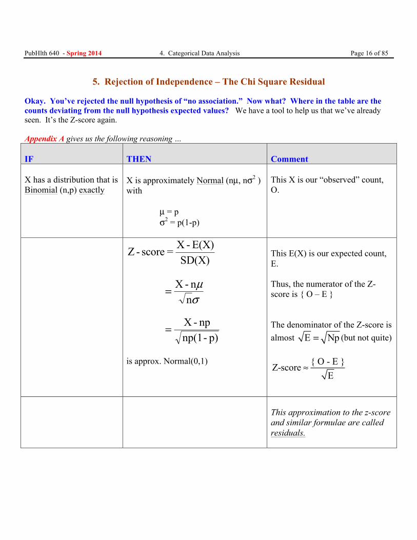
5. Rejection of Independence – The Chi Square Residual Okay. You’ve rejected the null hypothesis of “no association.” Now what? Where in the table are the counts deviating from the null hypothesis expected values? We have a tool to help us that we’ve already seen. It’s the Z-score again. Appendix A gives us the following reasoning … IF
THEN
Comment
X has a distribution that is Binomial (n,p) exactly
X is approximately Normal (nµ, nσ2 ) with µ = p σ2 = p(1-p)
This X is our “observed” count, O.
Z - score = X - E(X)
SD(X)
= X - nnµσ
= X - npnp(1- p)
is approx. Normal(0,1)
This E(X) is our expected count, E. Thus, the numerator of the Z-score is { O – E } The denominator of the Z-score is almost E Np= (but not quite)
{ O - E }Z-scoreE
≈
This approximation to the z-score and similar formulae are called residuals.
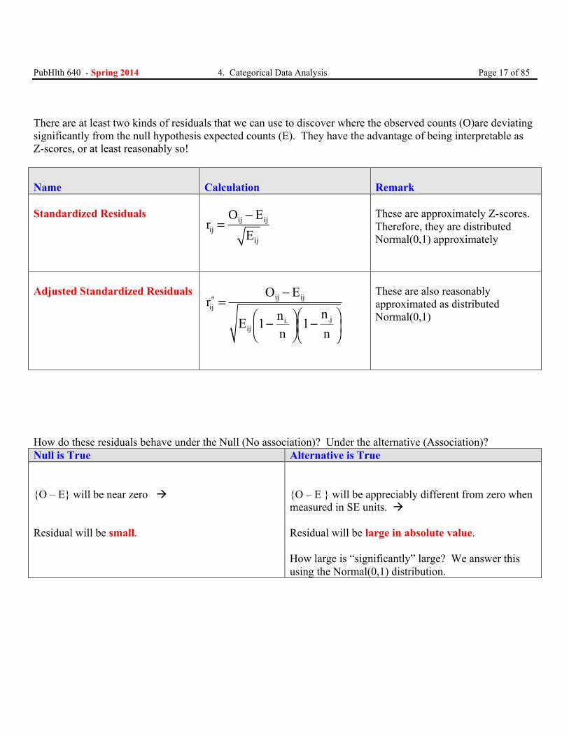
PubHlth 640 - Spring 2014 4. Categorical Data Analysis Page 17 of 85 There are at least two kinds of residuals that we can use to discover where the observed counts (O)are deviating significantly from the null hypothesis expected counts (E). They have the advantage of being interpretable as Z-scores, or at least reasonably so! Name
Calculation
Remark
Standardized Residuals
ij ij
ijij
O Er
E−
=
These are approximately Z-scores. Therefore, they are distributed Normal(0,1) approximately
Adjusted Standardized Residuals
ij ij
ij.ji.
ij
O Er
nnE 1 1n n
∗ −=
⎛ ⎞⎛ ⎞− −⎜ ⎟⎜ ⎟⎝ ⎠⎝ ⎠
These are also reasonably approximated as distributed Normal(0,1)
How do these residuals behave under the Null (No association)? Under the alternative (Association)? Null is True Alternative is True {O – E} will be near zero à Residual will be small.
{O – E } will be appreciably different from zero when measured in SE units. à Residual will be large in absolute value. How large is “significantly” large? We answer this using the Normal(0,1) distribution.
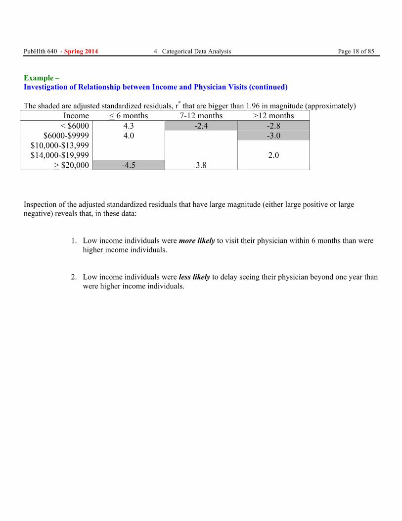
PubHlth 640 - Spring 2014 4. Categorical Data Analysis Page 18 of 85 Example – Investigation of Relationship between Income and Physician Visits (continued) The shaded are adjusted standardized residuals, r* that are bigger than 1.96 in magnitude (approximately)
Income < 6 months 7-12 months >12 months < $6000 4.3 -2.4 -2.8
$6000-$9999 4.0 -3.0 $10,000-$13,999 $14,000-$19,999 2.0
> $20,000 -4.5 3.8 Inspection of the adjusted standardized residuals that have large magnitude (either large positive or large negative) reveals that, in these data:
1. Low income individuals were more likely to visit their physician within 6 months than were higher income individuals.
2. Low income individuals were less likely to delay seeing their physician beyond one year than were higher income individuals.
PubHlth 640 - Spring 2014 4. Categorical Data Analysis Page 19 of 85
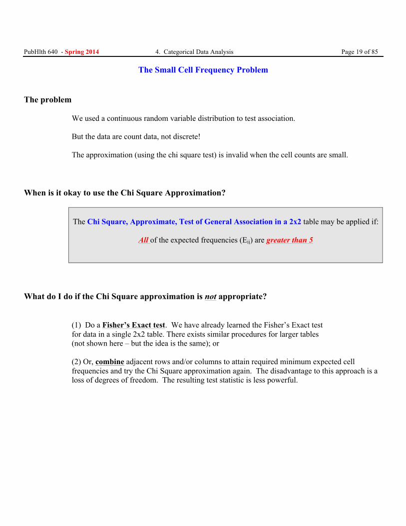
The Small Cell Frequency Problem The problem
We used a continuous random variable distribution to test association. But the data are count data, not discrete! The approximation (using the chi square test) is invalid when the cell counts are small.
When is it okay to use the Chi Square Approximation?
The Chi Square, Approximate, Test of General Association in a 2x2 table may be applied if:
All of the expected frequencies (Eij) are greater than 5
What do I do if the Chi Square approximation is not appropriate?
(1) Do a Fisher’s Exact test. We have already learned the Fisher’s Exact test for data in a single 2x2 table. There exists similar procedures for larger tables (not shown here – but the idea is the same); or (2) Or, combine adjacent rows and/or columns to attain required minimum expected cell frequencies and try the Chi Square approximation again. The disadvantage to this approach is a loss of degrees of freedom. The resulting test statistic is less powerful.
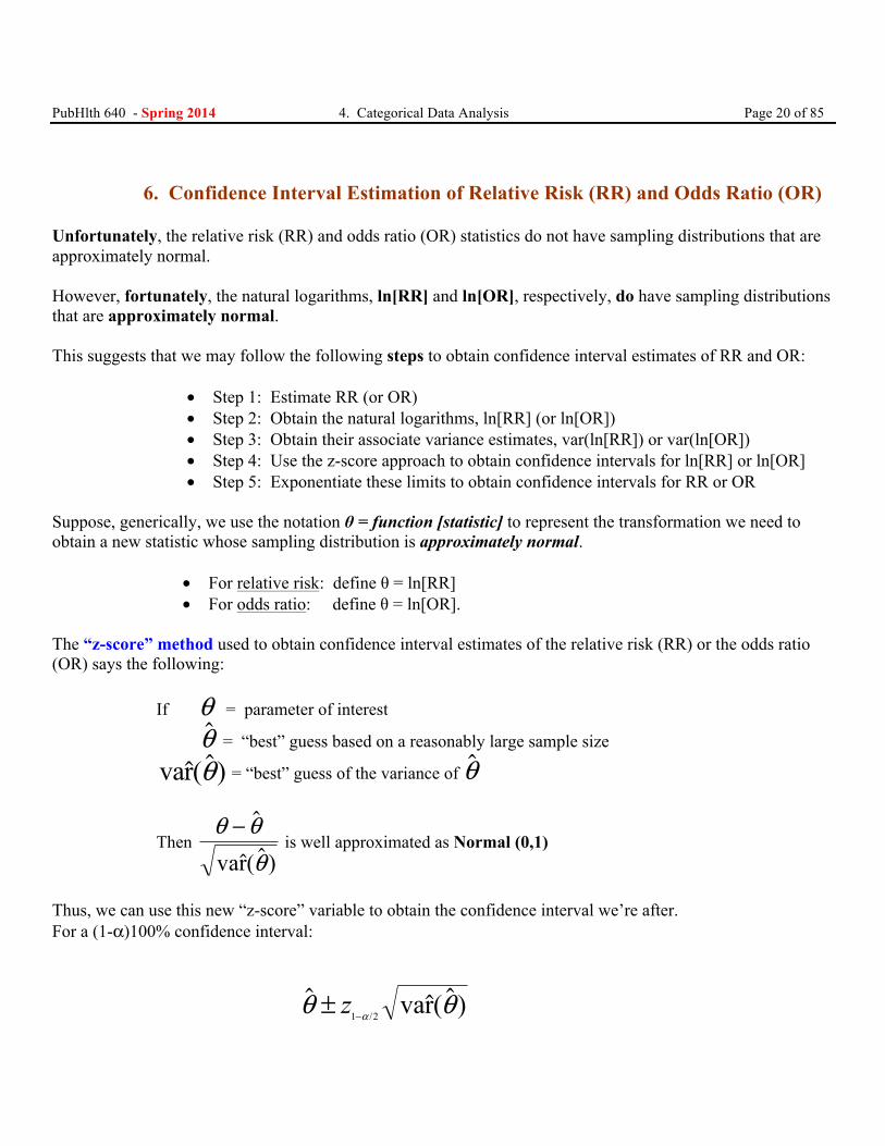
PubHlth 640 - Spring 2014 4. Categorical Data Analysis Page 20 of 85 6. Confidence Interval Estimation of Relative Risk (RR) and Odds Ratio (OR) Unfortunately, the relative risk (RR) and odds ratio (OR) statistics do not have sampling distributions that are approximately normal. However, fortunately, the natural logarithms, ln[RR] and ln[OR], respectively, do have sampling distributions that are approximately normal. This suggests that we may follow the following steps to obtain confidence interval estimates of RR and OR:
• Step 1: Estimate RR (or OR) • Step 2: Obtain the natural logarithms, ln[RR] (or ln[OR]) • Step 3: Obtain their associate variance estimates, var(ln[RR]) or var(ln[OR]) • Step 4: Use the z-score approach to obtain confidence intervals for ln[RR] or ln[OR] • Step 5: Exponentiate these limits to obtain confidence intervals for RR or OR
Suppose, generically, we use the notation θ = function [statistic] to represent the transformation we need to obtain a new statistic whose sampling distribution is approximately normal.
• For relative risk: define θ = ln[RR] • For odds ratio: define θ = ln[OR].
The “z-score” method used to obtain confidence interval estimates of the relative risk (RR) or the odds ratio (OR) says the following:
If θ = parameter of interest
θ = “best” guess based on a reasonably large sample size
var( )θ = “best” guess of the variance of θ
Then θ θ
θ−
var( ) is well approximated as Normal (0,1)
Thus, we can use this new “z-score” variable to obtain the confidence interval we’re after. For a (1-α)100% confidence interval:
var( )/θ θα± −z1 2
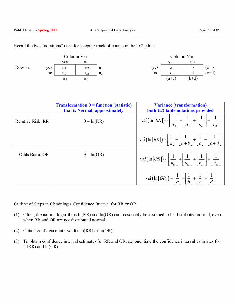
PubHlth 640 - Spring 2014 4. Categorical Data Analysis Page 21 of 85 Recall the two “notations” used for keeping track of counts in the 2x2 table: Column Var Column Var yes no yes no Row var yes n11 n12 n1. yes a b (a+b)
no n21 n22 n2. no c d (c+d) n.1 n.2 (a+c) (b+d) Transformation θ = function (statistic)
that is Normal, approximately Variance (transformation)
both 2x2 table notations provided
Relative Risk, RR
θ = ln(RR) [ ]( )11 1. 21 2.
1 1 1 1ˆvar ln RRn n n n
⎡ ⎤ ⎡ ⎤⎡ ⎤ ⎡ ⎤≈ − + −⎢ ⎥ ⎢ ⎥⎢ ⎥ ⎢ ⎥⎣ ⎦ ⎣ ⎦⎣ ⎦ ⎣ ⎦
[ ]( ) 1 1 1 1ˆvar ln RRa a b c c d
⎡ ⎤ ⎡ ⎤ ⎡ ⎤ ⎡ ⎤≈ − + −⎢ ⎥ ⎢ ⎥ ⎢ ⎥ ⎢ ⎥+ +⎣ ⎦ ⎣ ⎦ ⎣ ⎦ ⎣ ⎦
Odds Ratio, OR
θ = ln(OR)
[ ]( )11 12 21 22
1 1 1 1ˆvar ln ORn n n n⎡ ⎤ ⎡ ⎤ ⎡ ⎤ ⎡ ⎤
≈ + + +⎢ ⎥ ⎢ ⎥ ⎢ ⎥ ⎢ ⎥⎣ ⎦ ⎣ ⎦ ⎣ ⎦ ⎣ ⎦
[ ]( ) 1 1 1 1ˆvar ln ORa b c d
⎡ ⎤ ⎡ ⎤ ⎡ ⎤ ⎡ ⎤≈ + + +⎢ ⎥ ⎢ ⎥ ⎢ ⎥ ⎢ ⎥⎣ ⎦ ⎣ ⎦ ⎣ ⎦ ⎣ ⎦
Outline of Steps in Obtaining a Confidence Interval for RR or OR (1) Often, the natural logarithms ln(RR) and ln(OR) can reasonably be assumed to be distributed normal, even
when RR and OR are not distributed normal. (2) Obtain confidence interval for ln(RR) or ln(OR)
(3) To obtain confidence interval estimates for RR and OR, exponentiate the confidence interval estimates for
ln(RR) and ln(OR).
PubHlth 640 - Spring 2014 4. Categorical Data Analysis Page 22 of 85
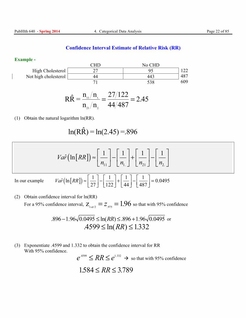
Confidence Interval Estimate of Relative Risk (RR)
Example -
CHD No CHD 122 487 609
High Cholesterol 27 95 Not high cholesterol 44 443
71 538
RR = n nn n11 1.
21 2.
.= =27 12244 487
2 45
(1) Obtain the natural logarithm ln(RR).
ln(RR) = ln(2.45) =.896
[ ]( )11 1. 21 2.
1 1 1 1ˆ lnVar RRn n n n
⎡ ⎤ ⎡ ⎤⎡ ⎤ ⎡ ⎤≈ − + −⎢ ⎥ ⎢ ⎥⎢ ⎥ ⎢ ⎥⎣ ⎦ ⎣ ⎦⎣ ⎦ ⎣ ⎦
In our example [ ]( ) 1 1 1 1ˆ ln 0.049527 122 44 487
Var RR ⎡ ⎤ ⎡ ⎤ ⎡ ⎤ ⎡ ⎤≈ − + − =⎢ ⎥ ⎢ ⎥ ⎢ ⎥ ⎢ ⎥⎣ ⎦ ⎣ ⎦ ⎣ ⎦ ⎣ ⎦
(2) Obtain confidence interval for ln(RR)
For a 95% confidence interval, z1- /2α = =z. .975 196 so that with 95% confidence .896 1.96 0.0495 ln( ) .896 1.96 0.0495RR− ≤ ≤ + or
. ln( ) .4599 1332≤ ≤RR
(3) Exponentiate .4599 and 1.332 to obtain the confidence interval for RR With 95% confidence.
e RR e. .4599 1 332≤ ≤ à so that with 95% confidence 1584 3789. .≤ ≤RR
PubHlth 640 - Spring 2014 4. Categorical Data Analysis Page 23 of 85
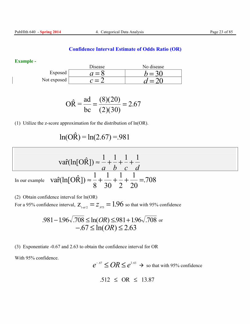
Confidence Interval Estimate of Odds Ratio (OR) Example -
Disease No disease
Exposed a = 8 b = 30 Not exposed c = 2 d = 20
OR = adbc
( )( )( )( )
.= =8 202 30
2 67
(1) Utilize the z-score approximation for the distribution of ln(OR).
ln(OR) = ln(2.67) =.981
var(ln[OR]) ≈ + + +1 1 1 1a b c d
In our example var(ln[OR]) .≈ + + + =18
130
12
120
708
(2) Obtain confidence interval for ln(OR) For a 95% confidence interval, z1- /2α = =z. .975 196 so that with 95% confidence
. . . ln( ) . . .981 196 708 981 196 708− ≤ ≤ +OR or
− ≤ ≤. ln( ) .67 2 63OR (3) Exponentiate -0.67 and 2.63 to obtain the confidence interval for OR With 95% confidence. e OR e− ≤ ≤. .67 2 63 à so that with 95% confidence .512 OR 13.87≤ ≤

PubHlth 640 - Spring 2014 4. Categorical Data Analysis Page 24 of 85
7. Strategies for Controlling Confounding We can control confounding at study design. • Restriction • Matching We can also control confounding analytically. • Stratification • Standardization • Matching
Restriction Restriction is the inclusion of only persons who are the same with respect to the confounder. • A study of males only will not produce results that are confounded by gender effects. • A study of non-smokers only will not produce results that are confounded by the effects of smoking. The advantage is a guarantee of control for confounding. However, there are also disadvantages. The sample size is limited and generalizability is reduced.
PubHlth 640 - Spring 2014 4. Categorical Data Analysis Page 25 of 85
Matching in a Cohort Study
Matching in a cohort study involves the following. • Enrollment of exposed persons without restriction. • Enrollment of unexposed only if they match exposed. Matching in a Case-Control Study In a case-control study the following occurs. • Enrollment of cases without restriction. • Enrollment of controls only if they match cases. Be careful!! Matching is not necessarily a good idea • In case-control studies, controls may be artificially similar to cases.
• Estimates of association may be spuriously low • If matching is related to exposure only, not confounding, then spurious confounding may be introduced • Sample size is reduced • Identical matched pairs provide no information Do not match • Most case-control studies. • On a variable that is intermediary. • When a large number of controls are available Consider matching
• In an experiment and some cohort studies • On some variables (age, sex, site)
PubHlth 640 - Spring 2014 4. Categorical Data Analysis Page 26 of 85
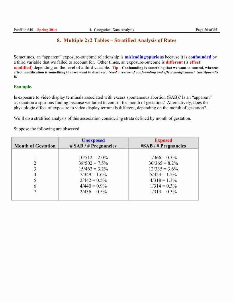
8. Multiple 2x2 Tables – Stratified Analysis of Rates Sometimes, an “apparent” exposure-outcome relationship is misleading/spurious because it is confounded by a third variable that we failed to account for. Other times, an exposure-outcome is different (is effect modified) depending on the level of a third variable. Tip – Confounding is something that we want to control, whereas effect modification is something that we want to discover. Need a review of confounding and effect modification? See Appendix E. Example. Is exposure to video display terminals associated with excess spontaneous abortion (SAB)? Is an “apparent” association a spurious finding because we failed to control for month of gestation? Alternatively, does the physiologic effect of exposure to video display terminals different, depending on the month of gestation?. We’ll do a stratified analysis of this association considering strata defined by month of gestation. Suppose the following are observed.
Unexposed Exposed Month of Gestation # SAB / # Pregnancies #SAB / # Pregnancies
1 10/512 = 2.0% 1/366 = 0.3% 2 38/502 = 7.5% 30/365 = 8.2% 3 15/462 = 3.2% 12/335 = 3.6% 4 7/449 = 1.6% 5/323 = 1.5% 5 2/442 = 0.5% 4/318 = 1.3% 6 4/440 = 0.9% 1/314 = 0.3% 7 2/436 = 0.5% 1/313 = 0.3%
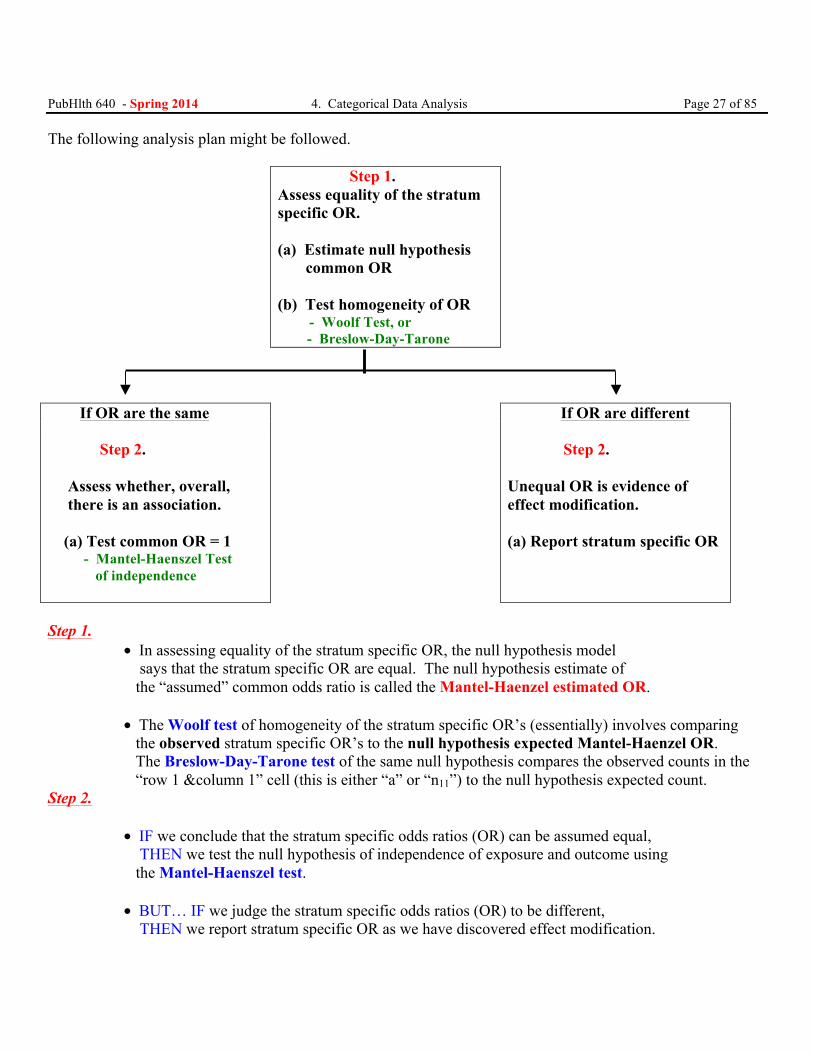
PubHlth 640 - Spring 2014 4. Categorical Data Analysis Page 27 of 85 The following analysis plan might be followed. Step 1.
Assess equality of the stratum specific OR. (a) Estimate null hypothesis common OR (b) Test homogeneity of OR - Woolf Test, or - Breslow-Day-Tarone
If OR are the same If OR are different Step 2. Assess whether, overall, there is an association. (a) Test common OR = 1 - Mantel-Haenszel Test of independence
Step 2. Unequal OR is evidence of effect modification. (a) Report stratum specific OR
Step 1. • In assessing equality of the stratum specific OR, the null hypothesis model says that the stratum specific OR are equal. The null hypothesis estimate of the “assumed” common odds ratio is called the Mantel-Haenzel estimated OR. • The Woolf test of homogeneity of the stratum specific OR’s (essentially) involves comparing the observed stratum specific OR’s to the null hypothesis expected Mantel-Haenzel OR. The Breslow-Day-Tarone test of the same null hypothesis compares the observed counts in the “row 1 &column 1” cell (this is either “a” or “n11”) to the null hypothesis expected count. Step 2. • IF we conclude that the stratum specific odds ratios (OR) can be assumed equal, THEN we test the null hypothesis of independence of exposure and outcome using the Mantel-Haenszel test. • BUT… IF we judge the stratum specific odds ratios (OR) to be different, THEN we report stratum specific OR as we have discovered effect modification.
PubHlth 640 - Spring 2014 4. Categorical Data Analysis Page 28 of 85
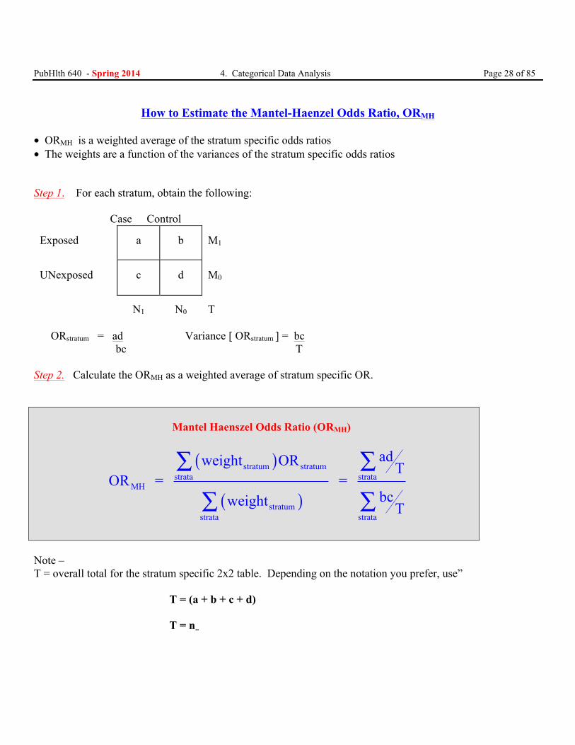
How to Estimate the Mantel-Haenzel Odds Ratio, ORMH • ORMH is a weighted average of the stratum specific odds ratios • The weights are a function of the variances of the stratum specific odds ratios Step 1. For each stratum, obtain the following:
Case Control Exposed
a
b
M1
UNexposed
c
d
M0
N1
N0
T
ORstratum = ad Variance [ ORstratum ] = bc bc T Step 2. Calculate the ORMH as a weighted average of stratum specific OR.
Mantel Haenszel Odds Ratio (ORMH)
( )
( )
stratum stratumstrata strata
MH
stratumstrata strata
adweight OR TOR = =
bcweight T
∑ ∑
∑ ∑
Note – T = overall total for the stratum specific 2x2 table. Depending on the notation you prefer, use” T = (a + b + c + d) T = n..
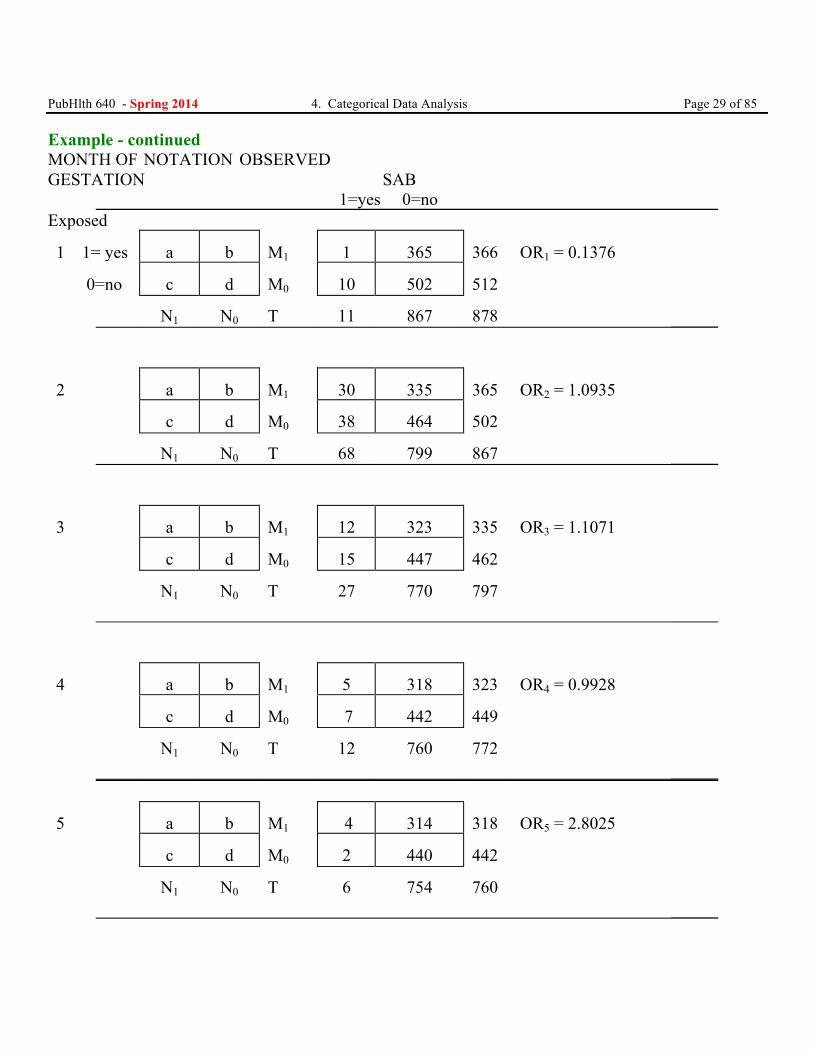
PubHlth 640 - Spring 2014 4. Categorical Data Analysis Page 29 of 85 Example - continued MONTH OF NOTATION OBSERVED GESTATION SAB 1=yes 0=no Exposed 1 1= yes
a
b
M1
1
365
366
OR1 = 0.1376
0=no
c
d
M0
10
502
512
N1
N0
T
11
867
878
2
a
b
M1
30
335
365
OR2 = 1.0935
c
d
M0
38
464
502
N1
N0
T
68
799
867
3
a
b
M1
12
323
335
OR3 = 1.1071
c
d
M0
15
447
462
N1
N0
T
27
770
797
4
a
b
M1
5
318
323
OR4 = 0.9928
c
d
M0
7
442
449
N1
N0
T
12
760
772
5
a
b
M1
4
314
318
OR5 = 2.8025
c
d
M0
2
440
442
N1
N0
T
6
754
760
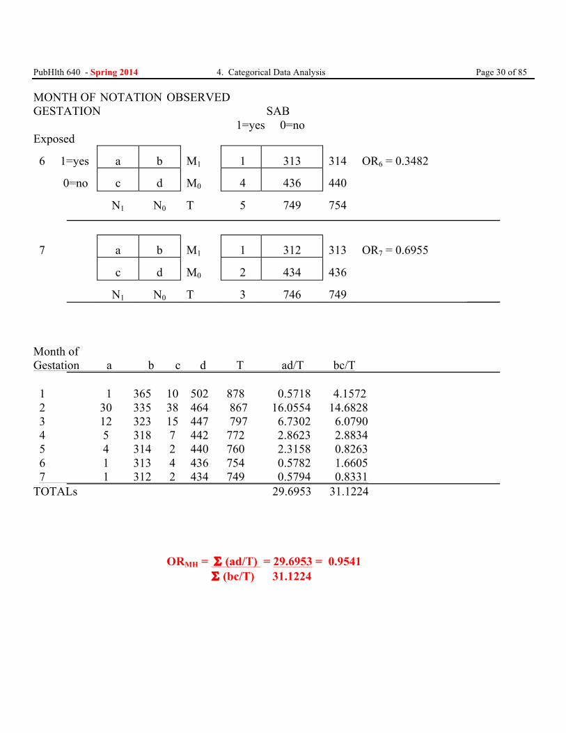
PubHlth 640 - Spring 2014 4. Categorical Data Analysis Page 30 of 85 MONTH OF NOTATION OBSERVED GESTATION SAB 1=yes 0=no Exposed 6 1=yes
a
b
M1
1
313
314
OR6 = 0.3482
0=no
c
d
M0
4
436
440
N1
N0
T
5
749
754
7
a
b
M1
1
312
313
OR7 = 0.6955
c
d
M0
2
434
436
N1
N0
T
3
746
749
Month of Gestation a b c d T ad/T bc/T 1 1 365 10 502 878 0.5718 4.1572 2 30 335 38 464 867 16.0554 14.6828 3 12 323 15 447 797 6.7302 6.0790 4 5 318 7 442 772 2.8623 2.8834 5 4 314 2 440 760 2.3158 0.8263 6 1 313 4 436 754 0.5782 1.6605 7 1 312 2 434 749 0.5794 0.8331 TOTALs 29.6953 31.1224 ORMH = Σ (ad/T) = 29.6953 = 0.9541
Σ (bc/T) 31.1224
PubHlth 640 - Spring 2014 4. Categorical Data Analysis Page 31 of 85
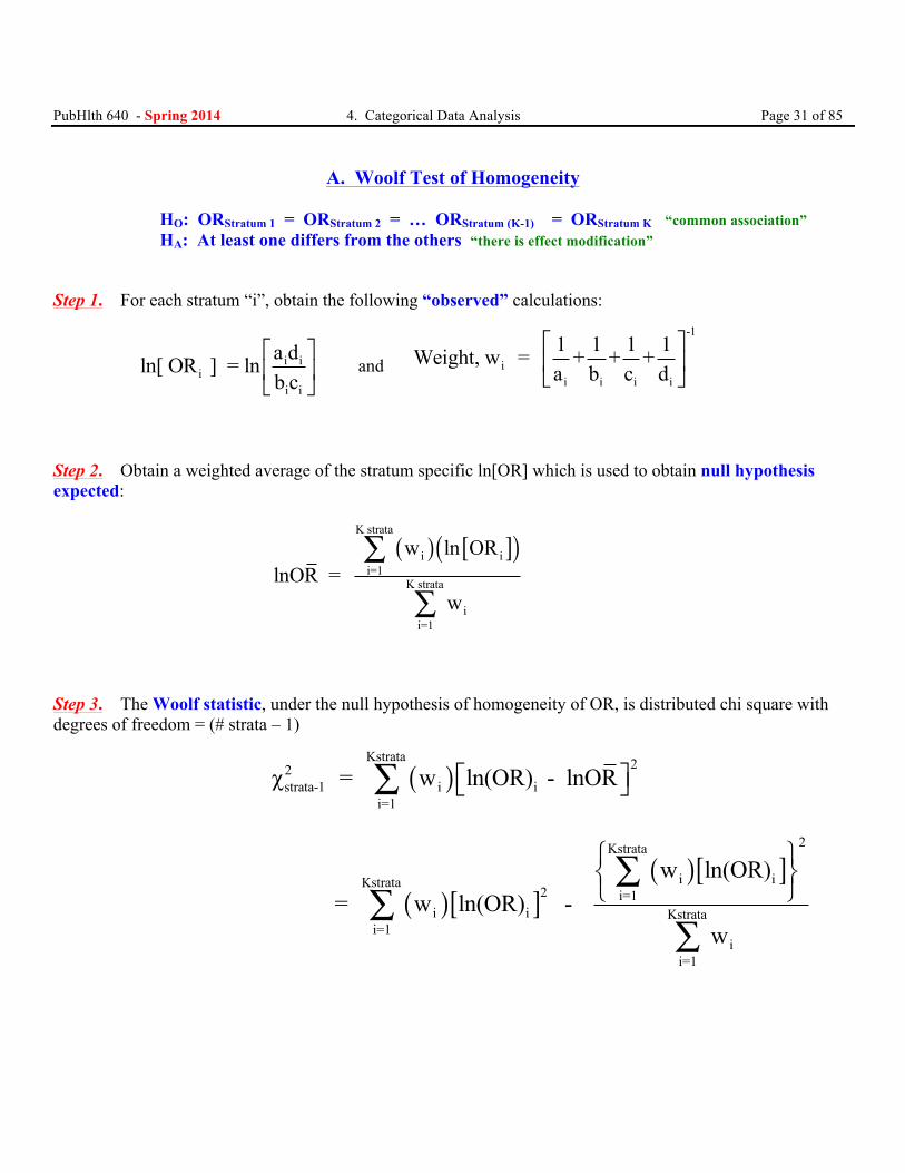
A. Woolf Test of Homogeneity
HO: ORStratum 1 = ORStratum 2 = … ORStratum (K-1) = ORStratum K “common association” HA: At least one differs from the others “there is effect modification”
Step 1. For each stratum “i”, obtain the following “observed” calculations:
i ii
i i
a dln[ OR ] = lnb c
⎡ ⎤⎢ ⎥⎣ ⎦
and
-1
ii i i i
1 1 1 1Weight, w = + + +a b c d⎡ ⎤⎢ ⎥⎣ ⎦
Step 2. Obtain a weighted average of the stratum specific ln[OR] which is used to obtain null hypothesis expected:
( ) [ ]( )
K strata
i ii=1
K strata
ii=1
w ln ORlnOR =
w
∑
∑
Step 3. The Woolf statistic, under the null hypothesis of homogeneity of OR, is distributed chi square with degrees of freedom = (# strata – 1)
( )Kstrata 22
strata-1 i ii=1
χ = w ln(OR) - lnOR⎡ ⎤⎣ ⎦∑
( )[ ]( )[ ]
2Kstrata
i iKstrata2 i=1
i i Kstratai=1
ii=1
w ln(OR) = w ln(OR) -
w
⎧ ⎫⎨ ⎬⎩ ⎭∑
∑∑
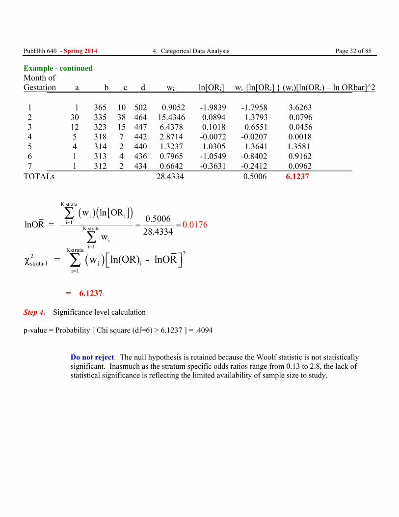
PubHlth 640 - Spring 2014 4. Categorical Data Analysis Page 32 of 85 Example - continued Month of Gestation a b c d wi ln[ORi] wi {ln[ORi] } (wi)[ln(ORi) – ln ORbar]^2 1 1 365 10 502 0.9052 -1.9839 -1.7958 3.6263 2 30 335 38 464 15.4346 0.0894 1.3793 0.0796 3 12 323 15 447 6.4378 0.1018 0.6551 0.0456 4 5 318 7 442 2.8714 -0.0072 -0.0207 0.0018 5 4 314 2 440 1.3237 1.0305 1.3641 1.3581 6 1 313 4 436 0.7965 -1.0549 -0.8402 0.9162 7 1 312 2 434 0.6642 -0.3631 -0.2412 0.0962 TOTALs 28.4334 0.5006 6.1237
( ) [ ]( )K strata
i ii=1
K strata
ii=1
w ln OR0.5006lnOR = 28.433
0 0 74w
. 1 6= =∑
∑
( )Kstrata 22
strata-1 i ii=1
χ = w ln(OR) - lnOR⎡ ⎤⎣ ⎦∑
= 6.1237 Step 4. Significance level calculation p-value = Probability [ Chi square (df=6) > 6.1237 ] = .4094
Do not reject. The null hypothesis is retained because the Woolf statistic is not statistically significant. Inasmuch as the stratum specific odds ratios range from 0.13 to 2.8, the lack of statistical significance is reflecting the limited availability of sample size to study.
PubHlth 640 - Spring 2014 4. Categorical Data Analysis Page 33 of 85
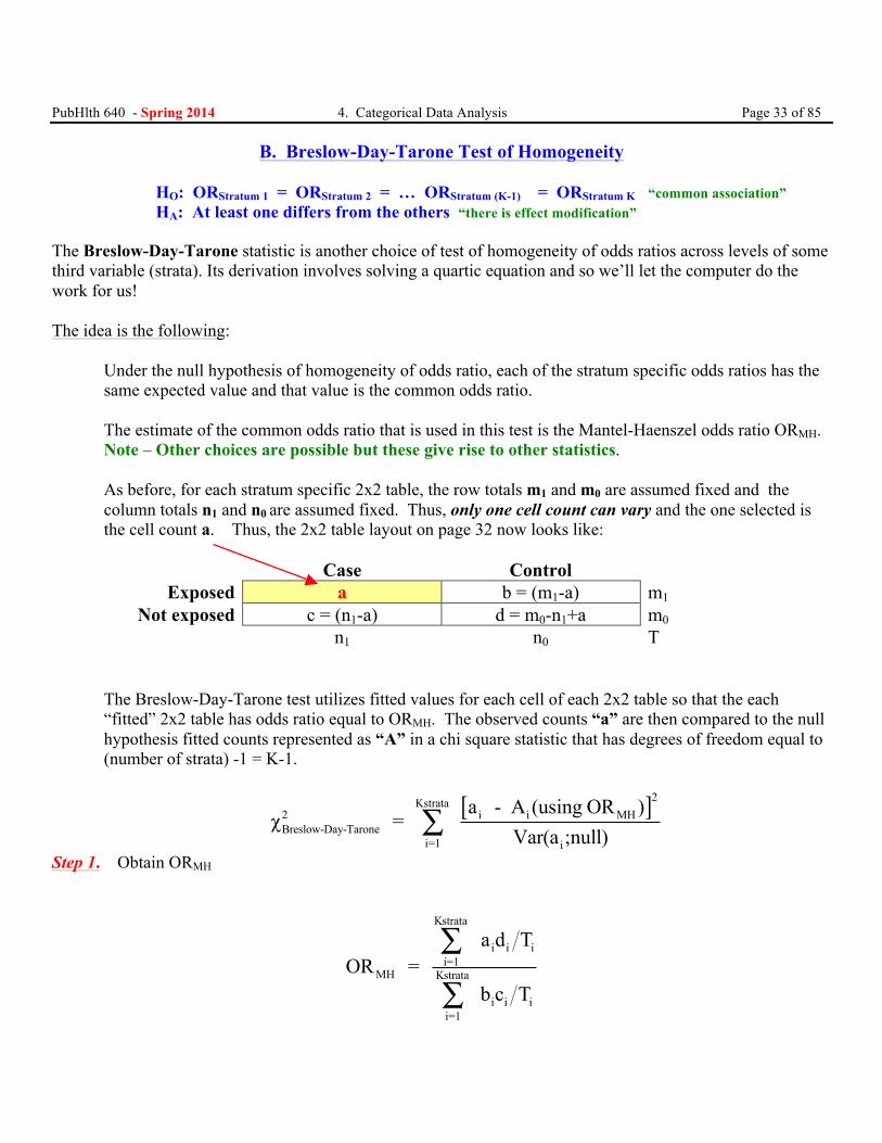
B. Breslow-Day-Tarone Test of Homogeneity HO: ORStratum 1 = ORStratum 2 = … ORStratum (K-1) = ORStratum K “common association” HA: At least one differs from the others “there is effect modification”
The Breslow-Day-Tarone statistic is another choice of test of homogeneity of odds ratios across levels of some third variable (strata). Its derivation involves solving a quartic equation and so we’ll let the computer do the work for us! The idea is the following:
Under the null hypothesis of homogeneity of odds ratio, each of the stratum specific odds ratios has the same expected value and that value is the common odds ratio. The estimate of the common odds ratio that is used in this test is the Mantel-Haenszel odds ratio ORMH. Note – Other choices are possible but these give rise to other statistics. As before, for each stratum specific 2x2 table, the row totals m1 and m0 are assumed fixed and the column totals n1 and n0 are assumed fixed. Thus, only one cell count can vary and the one selected is the cell count a. Thus, the 2x2 table layout on page 32 now looks like:
Case Control Exposed a b = (m1-a) m1
Not exposed c = (n1-a) d = m0-n1+a m0 n1 n0 T
The Breslow-Day-Tarone test utilizes fitted values for each cell of each 2x2 table so that the each “fitted” 2x2 table has odds ratio equal to ORMH. The observed counts “a” are then compared to the null hypothesis fitted counts represented as “A” in a chi square statistic that has degrees of freedom equal to (number of strata) -1 = K-1.
[ ]2Kstrata
2 i i MHBreslow-Day-Tarone
i=1 i
a - A (using OR )χ =
Var(a ;null)∑
Step 1. Obtain ORMH
Kstrata
i i ii=1
MH Kstrata
i i ii=1
a d TOR =
b c T
∑
∑
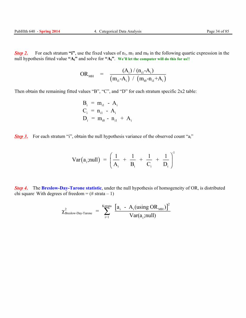
PubHlth 640 - Spring 2014 4. Categorical Data Analysis Page 34 of 85 Step 2. For each stratum “i”, use the fixed values of n1, m1 and m0 in the following quartic expression in the null hypothesis fitted value “Ai” and solve for “Ai”. We’ll let the computer will do this for us!!
( ) ( )i i1 i
MHi1 i i0 i1 i
(A ) / (n -A )OR = m -A / m -n +A
Then obtain the remaining fitted values “B”, “C”, and “D” for each stratum specific 2x2 table: i i1 iB = m - A i i1 iC = n - A i i0 i1 iD = m - n + A Step 3. For each stratum “i”, obtain the null hypothesis variance of the observed count “ai”
( )-1
ii i i i
1 1 1 1Var a ;null = + + + A B C D
⎛ ⎞⎜ ⎟⎝ ⎠
Step 4. The Breslow-Day-Tarone statistic, under the null hypothesis of homogeneity of OR, is distributed chi square. With degrees of freedom = (# strata – 1)
[ ]2Kstrata2 i i MHBreslow-Day-Tarone
i=1 i
a - A (using OR )χ =
Var(a ;null)∑
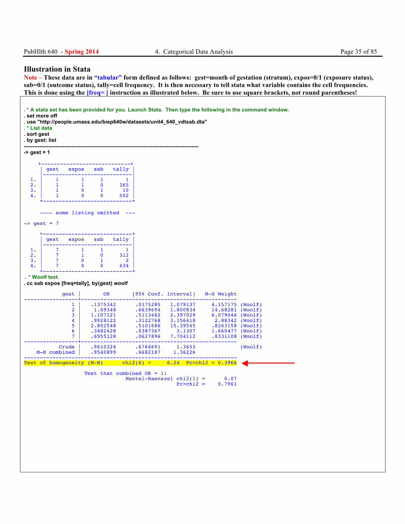
PubHlth 640 - Spring 2014 4. Categorical Data Analysis Page 35 of 85 Illustration in Stata Note – These data are in “tabular” form defined as follows: gest=month of gestation (stratum), expos=0/1 (exposure status), sab=0/1 (outcome status), tally=cell frequency. It is then necessary to tell stata what variable contains the cell frequencies. This is done using the [freq= ] instruction as illustrated below. Be sure to use square brackets, not round parentheses! . * A stata set has been provided for you. Launch Stata. Then type the following in the command window. . set more off . use "http://people.umass.edu/biep640w/datasets/unit4_640_vdtsab.dta" . * List data . sort gest . by gest: list --------------------------------------------------------------------------------------------------- -> gest = 1 +----------------------------+ | gest expos sab tally | |----------------------------| 1. | 1 1 1 1 | 2. | 1 1 0 365 | 3. | 1 0 1 10 | 4. | 1 0 0 502 | +----------------------------+ ---- some listing omitted --- -> gest = 7 +----------------------------+ | gest expos sab tally | |----------------------------| 1. | 7 1 1 1 | 2. | 7 1 0 312 | 3. | 7 0 1 2 | 4. | 7 0 0 434 | +----------------------------+ . * Woolf test. . cc sab expos [freq=tally], by(gest) woolf gest | OR [95% Conf. Interval] M-H Weight -----------------+------------------------------------------------- 1 | .1375342 .0175285 1.079137 4.157175 (Woolf) 2 | 1.09348 .6639694 1.800834 14.68281 (Woolf) 3 | 1.107121 .5113482 2.397029 6.079046 (Woolf) 4 | .9928122 .3122768 3.156418 2.88342 (Woolf) 5 | 2.802548 .5101686 15.39545 .8263158 (Woolf) 6 | .3482428 .0387367 3.1307 1.660477 (Woolf) 7 | .6955128 .0627896 7.704112 .8331108 (Woolf) -----------------+------------------------------------------------- Crude | .9610324 .6764691 1.3653 (Woolf) M-H combined | .9540899 .6682187 1.36226 ------------------------------------------------------------------- Test of homogeneity (M-H) chi2(6) = 6.24 Pr>chi2 = 0.3966 Test that combined OR = 1: Mantel-Haenszel chi2(1) = 0.07 Pr>chi2 = 0.7961
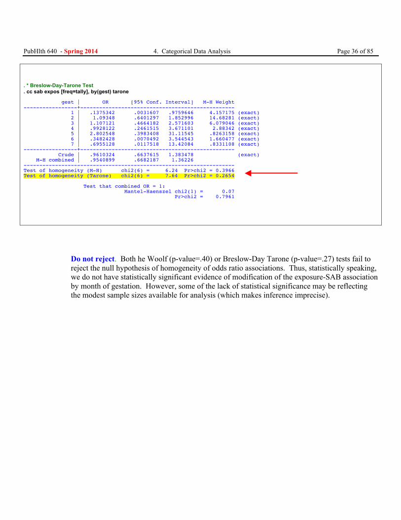
PubHlth 640 - Spring 2014 4. Categorical Data Analysis Page 36 of 85 . * Breslow-Day-Tarone Test . cc sab expos [freq=tally], by(gest) tarone gest | OR [95% Conf. Interval] M-H Weight -----------------+------------------------------------------------- 1 | .1375342 .0031607 .9759646 4.157175 (exact) 2 | 1.09348 .6401297 1.852996 14.68281 (exact) 3 | 1.107121 .4664182 2.571603 6.079046 (exact) 4 | .9928122 .2461515 3.671101 2.88342 (exact) 5 | 2.802548 .3983408 31.11545 .8263158 (exact) 6 | .3482428 .0070492 3.544543 1.660477 (exact) 7 | .6955128 .0117518 13.42084 .8331108 (exact) -----------------+------------------------------------------------- Crude | .9610324 .6637615 1.383478 (exact) M-H combined | .9540899 .6682187 1.36226 ------------------------------------------------------------------- Test of homogeneity (M-H) chi2(6) = 6.24 Pr>chi2 = 0.3966 Test of homogeneity (Tarone) chi2(6) = 7.64 Pr>chi2 = 0.2654 Test that combined OR = 1: Mantel-Haenszel chi2(1) = 0.07 Pr>chi2 = 0.7961
Do not reject. Both he Woolf (p-value=.40) or Breslow-Day Tarone (p-value=.27) tests fail to reject the null hypothesis of homogeneity of odds ratio associations. Thus, statistically speaking, we do not have statistically significant evidence of modification of the exposure-SAB association by month of gestation. However, some of the lack of statistical significance may be reflecting the modest sample sizes available for analysis (which makes inference imprecise).
PubHlth 640 - Spring 2014 4. Categorical Data Analysis Page 37 of 85
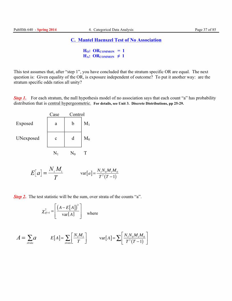
C. Mantel Haenszel Test of No Association HO: ORCOMMON = 1 HA: ORCOMMON ≠ 1
This test assumes that, after “step 1”, you have concluded that the stratum specific OR are equal. The next question is: Given equality of the OR, is exposure independent of outcome? To put it another way: are the stratum specific odds ratios all unity? Step 1. For each stratum, the null hypothesis model of no association says that each count “a” has probability distribution that is central hypergeometric. For details, see Unit 3. Discrete Distributions, pp 25-29.
Case Control Exposed
a
b
M1
UNexposed
c
d
M0
N1
N0
T
E a N MT
= 1 1 var a[ ] = N1N0M1M 0
T 2 T −1( )
Step 2. The test statistic will be the sum, over strata of the counts “a”.
χdf =12 =
A − E A[ ]( )2var A[ ]
⎡
⎣⎢⎢
⎤
⎦⎥⎥
where
A astrata
= ∑ E A[ ] = N1M1
T⎡⎣⎢
⎤⎦⎥strata
∑ var A[ ] = N1N0M1M 0
T 2 T −1( )⎡
⎣⎢
⎤
⎦⎥∑
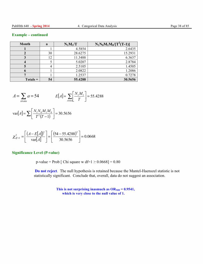
PubHlth 640 - Spring 2014 4. Categorical Data Analysis Page 38 of 85 Example – continued
Month a N1M1/T N1N0M1M0/[T2(T-1)] 1 1 4.5854 2.6435 2 30 28.6275 15.2931 3 12 11.3488 6.3637 4 5 5.0207 2.8784 5 4 2.5105 1.4505 6 1 2.0822 1.2086 7 1 1.2537 0.7278 Totals = 54 55.4288 30.5656
54strata
A a= =∑ [ ] 4288.5511 =⎥⎦⎤
⎢⎣⎡= ∑
strata TMNAE
[ ] ( ) 5656.301
var 20101 =⎥⎦
⎤⎢⎣
⎡−
=∑ TTMMNNA
[ ]( )[ ]
( ) 0668.05656.304288.5554
var
2221 =⎥
⎦
⎤⎢⎣
⎡ −=⎥⎦
⎤⎢⎣
⎡ −== AAEA
dfχ
Significance Level (P-value)
p-value = Prob [ Chi square w df=1 > 0.0668] = 0.80 Do not reject. The null hypothesis is retained because the Mantel-Haenszel statistic is not statistically significant. Conclude that, overall, data do not suggest an association. This is not surprising inasmuch as ORMH = 0.9541, which is very close to the null value of 1.
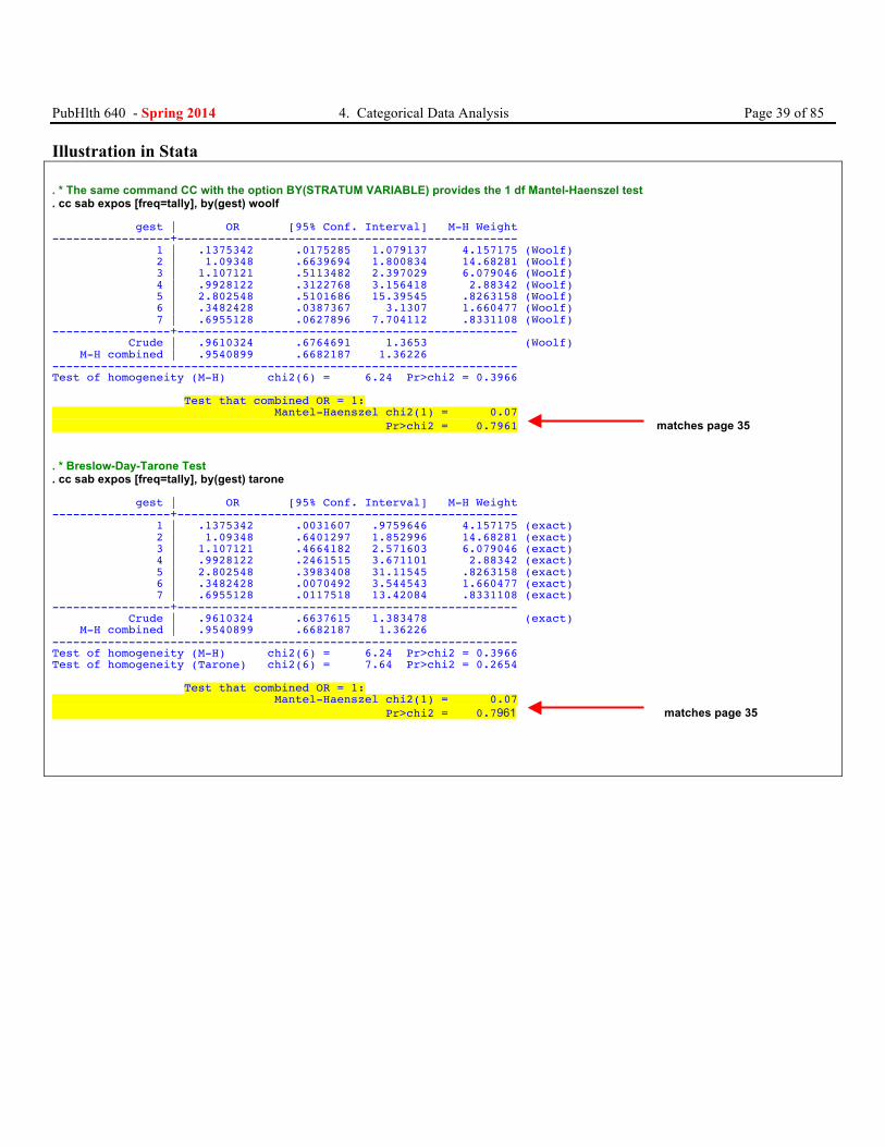
PubHlth 640 - Spring 2014 4. Categorical Data Analysis Page 39 of 85 Illustration in Stata . * The same command CC with the option BY(STRATUM VARIABLE) provides the 1 df Mantel-Haenszel test . cc sab expos [freq=tally], by(gest) woolf gest | OR [95% Conf. Interval] M-H Weight -----------------+------------------------------------------------- 1 | .1375342 .0175285 1.079137 4.157175 (Woolf) 2 | 1.09348 .6639694 1.800834 14.68281 (Woolf) 3 | 1.107121 .5113482 2.397029 6.079046 (Woolf) 4 | .9928122 .3122768 3.156418 2.88342 (Woolf) 5 | 2.802548 .5101686 15.39545 .8263158 (Woolf) 6 | .3482428 .0387367 3.1307 1.660477 (Woolf) 7 | .6955128 .0627896 7.704112 .8331108 (Woolf) -----------------+------------------------------------------------- Crude | .9610324 .6764691 1.3653 (Woolf) M-H combined | .9540899 .6682187 1.36226 ------------------------------------------------------------------- Test of homogeneity (M-H) chi2(6) = 6.24 Pr>chi2 = 0.3966 Test that combined OR = 1: Mantel-Haenszel chi2(1) = 0.07 Pr>chi2 = 0.7961 matches page 35 . * Breslow-Day-Tarone Test . cc sab expos [freq=tally], by(gest) tarone gest | OR [95% Conf. Interval] M-H Weight -----------------+------------------------------------------------- 1 | .1375342 .0031607 .9759646 4.157175 (exact) 2 | 1.09348 .6401297 1.852996 14.68281 (exact) 3 | 1.107121 .4664182 2.571603 6.079046 (exact) 4 | .9928122 .2461515 3.671101 2.88342 (exact) 5 | 2.802548 .3983408 31.11545 .8263158 (exact) 6 | .3482428 .0070492 3.544543 1.660477 (exact) 7 | .6955128 .0117518 13.42084 .8331108 (exact) -----------------+------------------------------------------------- Crude | .9610324 .6637615 1.383478 (exact) M-H combined | .9540899 .6682187 1.36226 ------------------------------------------------------------------- Test of homogeneity (M-H) chi2(6) = 6.24 Pr>chi2 = 0.3966 Test of homogeneity (Tarone) chi2(6) = 7.64 Pr>chi2 = 0.2654 Test that combined OR = 1: Mantel-Haenszel chi2(1) = 0.07 Pr>chi2 = 0.7961 matches page 35
PubHlth 640 - Spring 2014 4. Categorical Data Analysis Page 40 of 85
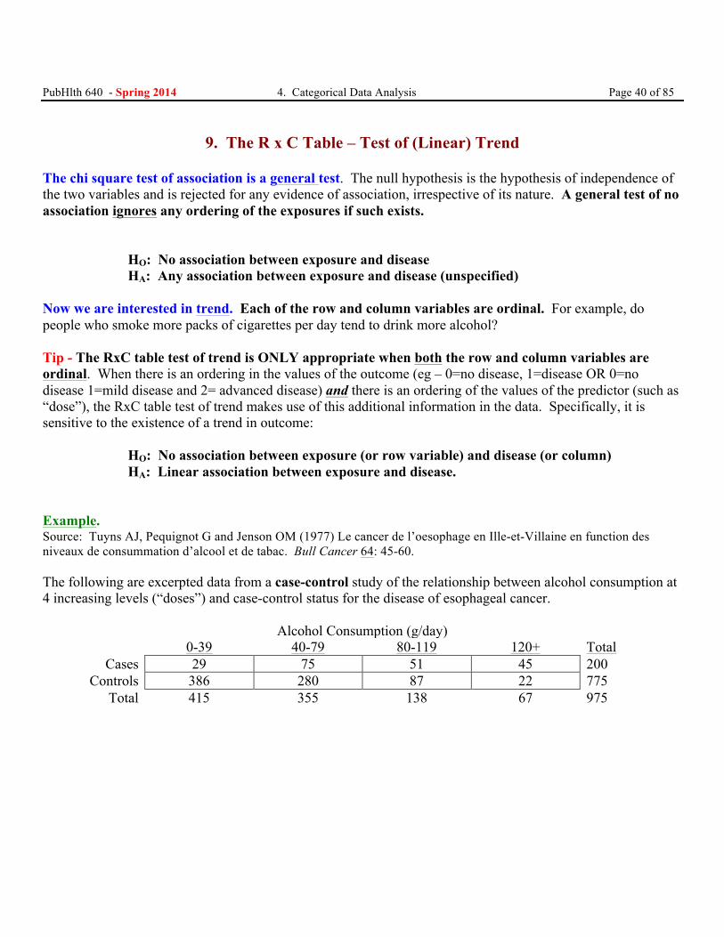
9. The R x C Table – Test of (Linear) Trend
The chi square test of association is a general test. The null hypothesis is the hypothesis of independence of the two variables and is rejected for any evidence of association, irrespective of its nature. A general test of no association ignores any ordering of the exposures if such exists.
HO: No association between exposure and disease HA: Any association between exposure and disease (unspecified)
Now we are interested in trend. Each of the row and column variables are ordinal. For example, do people who smoke more packs of cigarettes per day tend to drink more alcohol? Tip - The RxC table test of trend is ONLY appropriate when both the row and column variables are ordinal. When there is an ordering in the values of the outcome (eg – 0=no disease, 1=disease OR 0=no disease 1=mild disease and 2= advanced disease) and there is an ordering of the values of the predictor (such as “dose”), the RxC table test of trend makes use of this additional information in the data. Specifically, it is sensitive to the existence of a trend in outcome:
HO: No association between exposure (or row variable) and disease (or column) HA: Linear association between exposure and disease.
Example. Source: Tuyns AJ, Pequignot G and Jenson OM (1977) Le cancer de l’oesophage en Ille-et-Villaine en function des niveaux de consummation d’alcool et de tabac. Bull Cancer 64: 45-60. The following are excerpted data from a case-control study of the relationship between alcohol consumption at 4 increasing levels (“doses”) and case-control status for the disease of esophageal cancer.
Alcohol Consumption (g/day) 0-39 40-79 80-119 120+ Total
Cases 29 75 51 45 200 Controls 386 280 87 22 775
Total 415 355 138 67 975
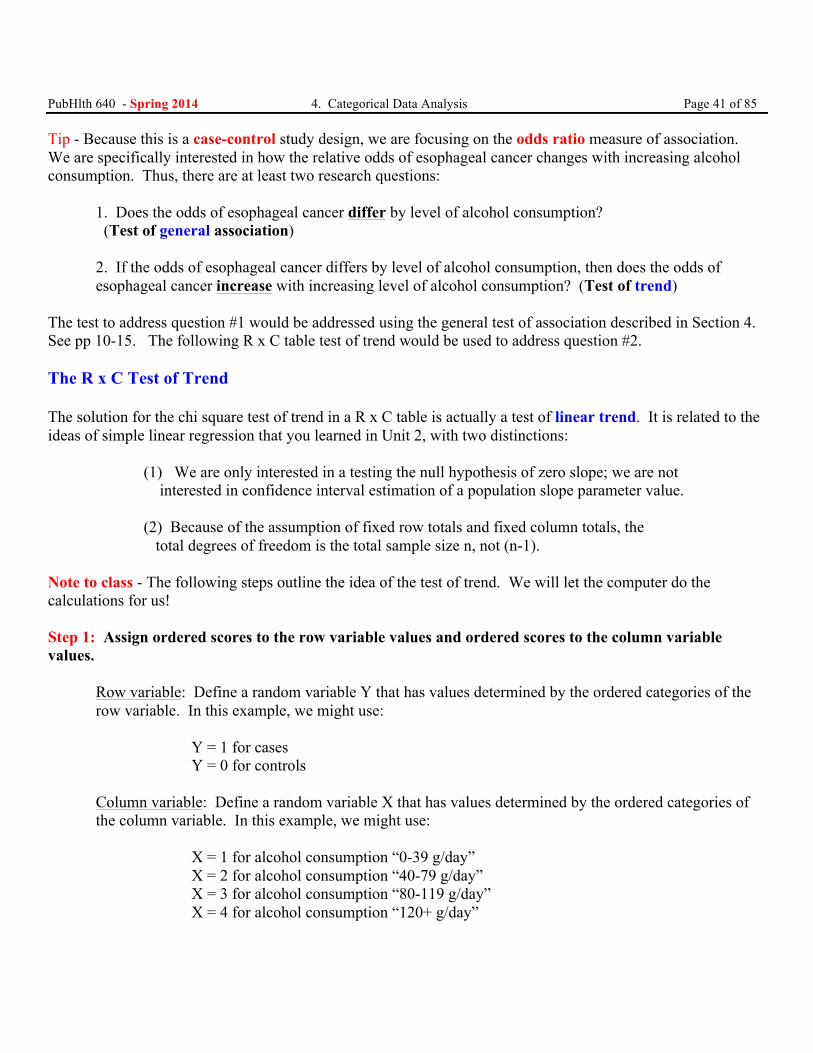
PubHlth 640 - Spring 2014 4. Categorical Data Analysis Page 41 of 85 Tip - Because this is a case-control study design, we are focusing on the odds ratio measure of association. We are specifically interested in how the relative odds of esophageal cancer changes with increasing alcohol consumption. Thus, there are at least two research questions:
1. Does the odds of esophageal cancer differ by level of alcohol consumption? (Test of general association) 2. If the odds of esophageal cancer differs by level of alcohol consumption, then does the odds of esophageal cancer increase with increasing level of alcohol consumption? (Test of trend)
The test to address question #1 would be addressed using the general test of association described in Section 4. See pp 10-15. The following R x C table test of trend would be used to address question #2. The R x C Test of Trend The solution for the chi square test of trend in a R x C table is actually a test of linear trend. It is related to the ideas of simple linear regression that you learned in Unit 2, with two distinctions:
(1) We are only interested in a testing the null hypothesis of zero slope; we are not interested in confidence interval estimation of a population slope parameter value. (2) Because of the assumption of fixed row totals and fixed column totals, the total degrees of freedom is the total sample size n, not (n-1).
Note to class - The following steps outline the idea of the test of trend. We will let the computer do the calculations for us! Step 1: Assign ordered scores to the row variable values and ordered scores to the column variable values.
Row variable: Define a random variable Y that has values determined by the ordered categories of the row variable. In this example, we might use:
Y = 1 for cases Y = 0 for controls
Column variable: Define a random variable X that has values determined by the ordered categories of the column variable. In this example, we might use:
X = 1 for alcohol consumption “0-39 g/day” X = 2 for alcohol consumption “40-79 g/day” X = 3 for alcohol consumption “80-119 g/day” X = 4 for alcohol consumption “120+ g/day”
PubHlth 640 - Spring 2014 4. Categorical Data Analysis Page 42 of 85
Tip!
It doesn’t matter which you call “X” and which you call “Y” Mostly, it doesn’t matter what scores you use as long as they are equally spaced.
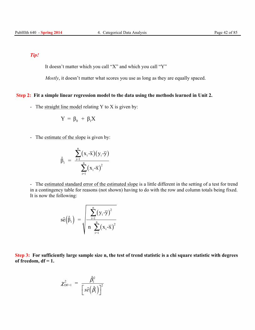
Step 2: Fit a simple linear regression model to the data using the methods learned in Unit 2.
- The straight line model relating Y to X is given by:
0 1Y = β + β X - The estimate of the slope is given by:
( )( )
( )
n
i ii=1
1 n2
ii=1
x -x y -yβ̂ =
x -x
∑
∑
- The estimated standard error of the estimated slope is a little different in the setting of a test for trend in a contingency table for reasons (not shown) having to do with the row and column totals being fixed. It is now the following:
( )( )
( )
n2
ii=1
1 n2
ii=1
y -yˆˆse β =
n x -x
∑
∑
Step 3: For sufficiently large sample size n, the test of trend statistic is a chi square statistic with degrees of freedom, df = 1.
( )2
2 1DF=1 2
1
ˆ =
ˆˆse
βχβ⎡ ⎤
⎣ ⎦
PubHlth 640 - Spring 2014 4. Categorical Data Analysis Page 43 of 85
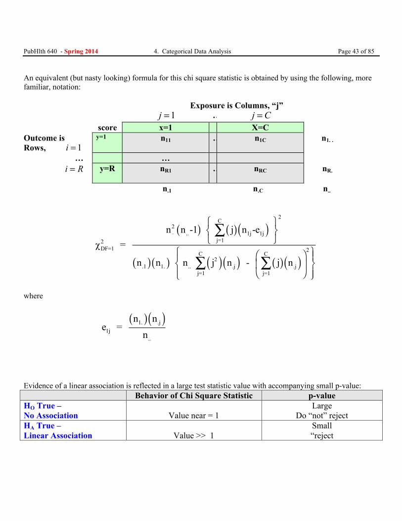
An equivalent (but nasty looking) formula for this chi square statistic is obtained by using the following, more familiar, notation: Exposure is Columns, “j” j =1 … j C= score x=1 X=C Outcome is Rows, i = 1
y=1 n11 … n1C n1. .
… … i R= y=R
nR1 … nRC nR.
n.1 n.C n..
( ) ( )( )
( )( ) ( )( ) ( )( )
..
2C
2.. 1j 1j
j=12DF=1 2
C C2
.1 1. .. .j .jj=1 j=1
n n -1 j n -e χ =
n n n j n - j n
⎧ ⎫⎨ ⎬⎩ ⎭
⎧ ⎫⎛ ⎞⎪ ⎪⎨ ⎬⎜ ⎟
⎝ ⎠⎪ ⎪⎩ ⎭
∑
∑ ∑
where
( )( )1. .j
1j..
n ne =
n
Evidence of a linear association is reflected in a large test statistic value with accompanying small p-value: Behavior of Chi Square Statistic p-value HO True – No Association
Value near = 1
Large Do “not” reject
HA True – Linear Association
Value >> 1
Small “reject
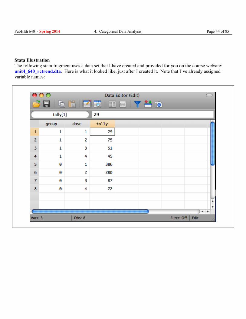
PubHlth 640 - Spring 2014 4. Categorical Data Analysis Page 44 of 85 Stata Illustration The following stata fragment uses a data set that I have created and provided for you on the course website: unit4_640_rctrend.dta. Here is what it looked like, just after I created it. Note that I’ve already assigned variable names:
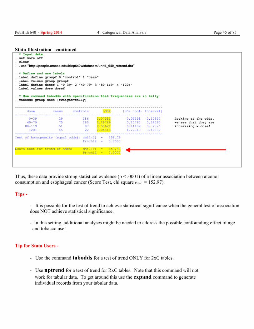
PubHlth 640 - Spring 2014 4. Categorical Data Analysis Page 45 of 85 Stata Illustration - continued . * Input data . set more off . clear . . use "http://people.umass.edu/biep640w/datasets/unit4_640_rctrend.dta" . * Define and use labels . label define groupf 0 "control" 1 "case" . label values group groupf . label define dosef 1 "0-39" 2 "40-79" 3 "80-119" 4 "120+" . label values dose dosef . * Use command tabodds with specification that frequencies are in tally . tabodds group dose [fweight=tally] -------------------------------------------------------------------------- dose | cases controls odds [95% Conf. Interval] ------------+------------------------------------------------------------- 0-39 | 29 386 0.07513 0.05151 0.10957 Looking at the odds, 40-79 | 75 280 0.26786 0.20760 0.34560 we see that they are 80-119 | 51 87 0.58621 0.41489 0.82826 increasing w dose! 120+ | 45 22 2.04545 1.22843 3.40587 -------------------------------------------------------------------------- Test of homogeneity (equal odds): chi2(3) = 158.79 Pr>chi2 = 0.0000 Score test for trend of odds: chi2(1) = 152.97 Pr>chi2 = 0.0000
Thus, these data provide strong statistical evidence (p < .0001) of a linear association between alcohol consumption and esophageal cancer (Score Test, chi square DF=1 = 152.97). Tips -
- It is possible for the test of trend to achieve statistical significance when the general test of association does NOT achieve statistical significance. - In this setting, additional analyses might be needed to address the possible confounding effect of age and tobacco use!
Tip for Stata Users -
- Use the command tabodds for a test of trend ONLY for 2xC tables. - Use nptrend for a test of trend for RxC tables. Note that this command will not work for tabular data. To get around this use the expand command to generate individual records from your tabular data.
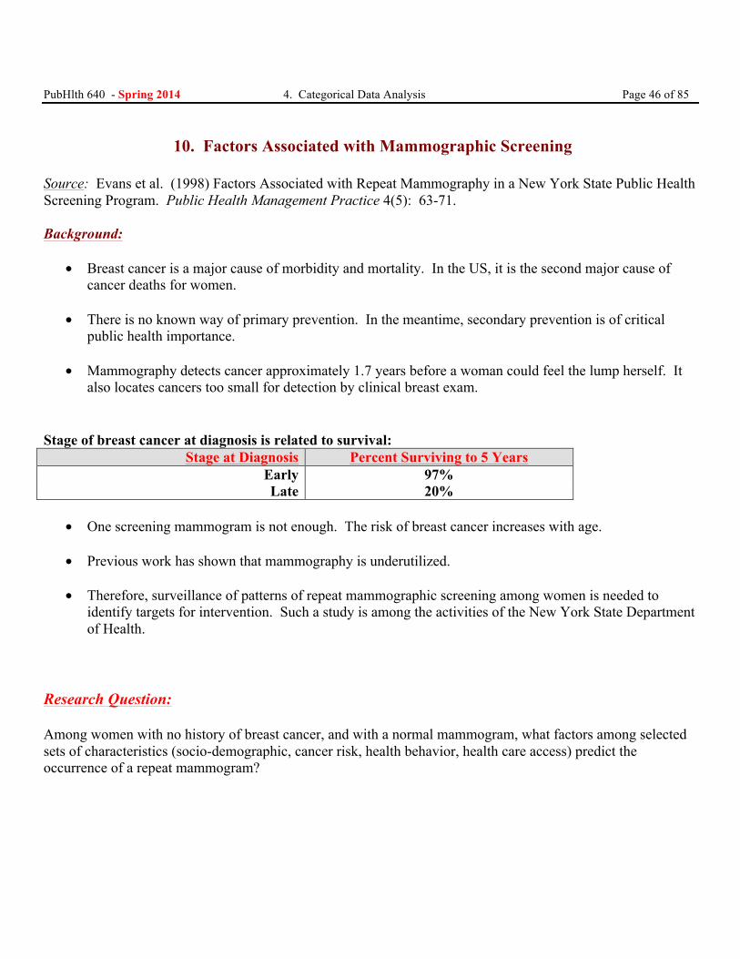
PubHlth 640 - Spring 2014 4. Categorical Data Analysis Page 46 of 85 10. Factors Associated with Mammographic Screening Source: Evans et al. (1998) Factors Associated with Repeat Mammography in a New York State Public Health Screening Program. Public Health Management Practice 4(5): 63-71. Background:
• Breast cancer is a major cause of morbidity and mortality. In the US, it is the second major cause of cancer deaths for women.
• There is no known way of primary prevention. In the meantime, secondary prevention is of critical
public health importance.
• Mammography detects cancer approximately 1.7 years before a woman could feel the lump herself. It also locates cancers too small for detection by clinical breast exam.
Stage of breast cancer at diagnosis is related to survival:
Stage at Diagnosis Percent Surviving to 5 Years Early 97% Late 20%
• One screening mammogram is not enough. The risk of breast cancer increases with age.
• Previous work has shown that mammography is underutilized.
• Therefore, surveillance of patterns of repeat mammographic screening among women is needed to
identify targets for intervention. Such a study is among the activities of the New York State Department of Health.
Research Question: Among women with no history of breast cancer, and with a normal mammogram, what factors among selected sets of characteristics (socio-demographic, cancer risk, health behavior, health care access) predict the occurrence of a repeat mammogram?
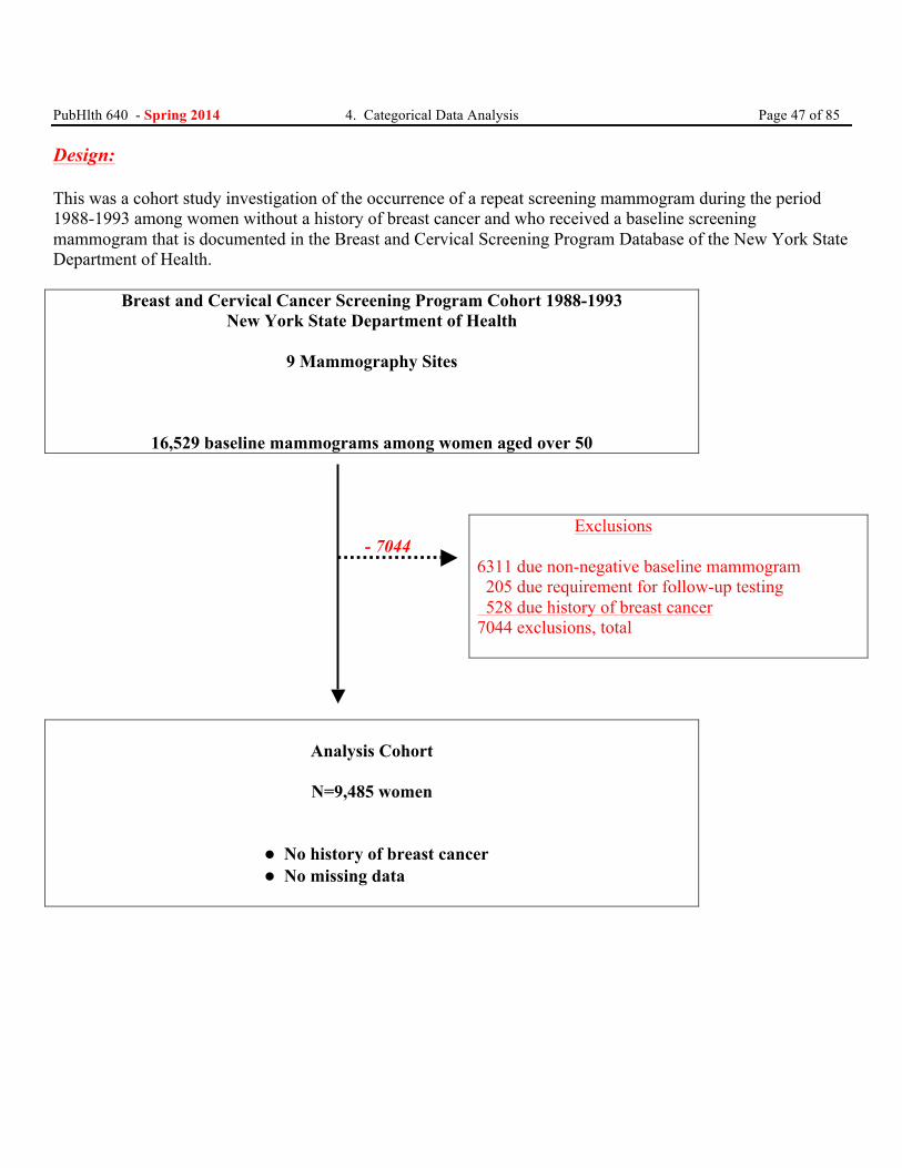
PubHlth 640 - Spring 2014 4. Categorical Data Analysis Page 47 of 85 Design: This was a cohort study investigation of the occurrence of a repeat screening mammogram during the period 1988-1993 among women without a history of breast cancer and who received a baseline screening mammogram that is documented in the Breast and Cervical Screening Program Database of the New York State Department of Health.
Breast and Cervical Cancer Screening Program Cohort 1988-1993 New York State Department of Health
9 Mammography Sites
16,529 baseline mammograms among women aged over 50
- 7044
Exclusions 6311 due non-negative baseline mammogram 205 due requirement for follow-up testing 528 due history of breast cancer 7044 exclusions, total
Analysis Cohort
N=9,485 women
• No history of breast cancer • No missing data
PubHlth 640 - Spring 2014 4. Categorical Data Analysis Page 48 of 85
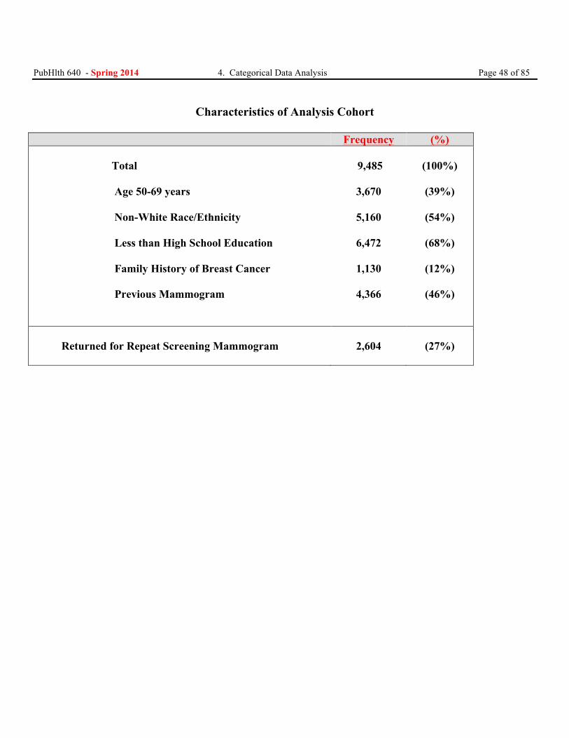
Characteristics of Analysis Cohort
Frequency (%) Total Age 50-69 years
Non-White Race/Ethnicity Less than High School Education Family History of Breast Cancer Previous Mammogram
9,485
3,670
5,160
6,472
1,130
4,366
(100%)
(39%)
(54%)
(68%)
(12%)
(46%)
Returned for Repeat Screening Mammogram
2,604
(27%)
PubHlth 640 - Spring 2014 4. Categorical Data Analysis Page 49 of 85
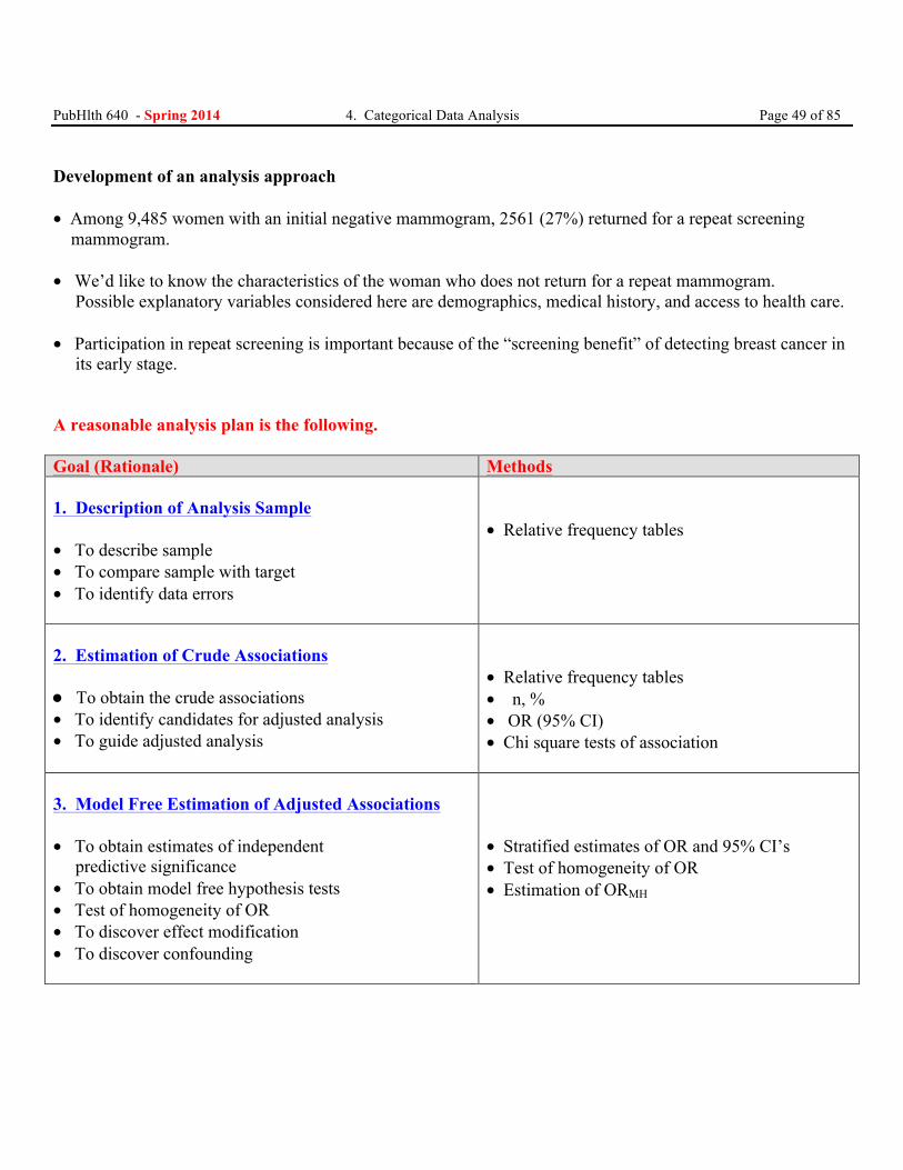
Development of an analysis approach • Among 9,485 women with an initial negative mammogram, 2561 (27%) returned for a repeat screening mammogram. • We’d like to know the characteristics of the woman who does not return for a repeat mammogram. Possible explanatory variables considered here are demographics, medical history, and access to health care. • Participation in repeat screening is important because of the “screening benefit” of detecting breast cancer in its early stage. A reasonable analysis plan is the following. Goal (Rationale) Methods 1. Description of Analysis Sample • To describe sample • To compare sample with target • To identify data errors
• Relative frequency tables
2. Estimation of Crude Associations • To obtain the crude associations • To identify candidates for adjusted analysis • To guide adjusted analysis
• Relative frequency tables • n, % • OR (95% CI) • Chi square tests of association
3. Model Free Estimation of Adjusted Associations • To obtain estimates of independent predictive significance • To obtain model free hypothesis tests • Test of homogeneity of OR • To discover effect modification • To discover confounding
• Stratified estimates of OR and 95% CI’s • Test of homogeneity of OR • Estimation of ORMH
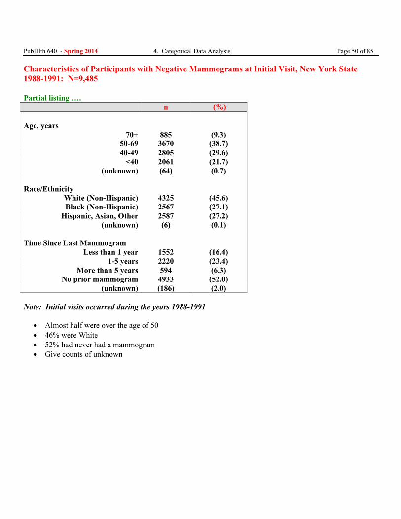
PubHlth 640 - Spring 2014 4. Categorical Data Analysis Page 50 of 85 Characteristics of Participants with Negative Mammograms at Initial Visit, New York State 1988-1991: N=9,485 Partial listing …. n (%) Age, years
70+ 885 (9.3) 50-69 3670 (38.7) 40-49 2805 (29.6)
<40 2061 (21.7) (unknown) (64) (0.7)
Race/Ethnicity
White (Non-Hispanic) 4325 (45.6) Black (Non-Hispanic) 2567 (27.1)
Hispanic, Asian, Other 2587 (27.2) (unknown) (6) (0.1)
Time Since Last Mammogram
Less than 1 year 1552 (16.4) 1-5 years 2220 (23.4)
More than 5 years 594 (6.3) No prior mammogram 4933 (52.0)
(unknown) (186) (2.0) Note: Initial visits occurred during the years 1988-1991 • Almost half were over the age of 50 • 46% were White • 52% had never had a mammogram • Give counts of unknown
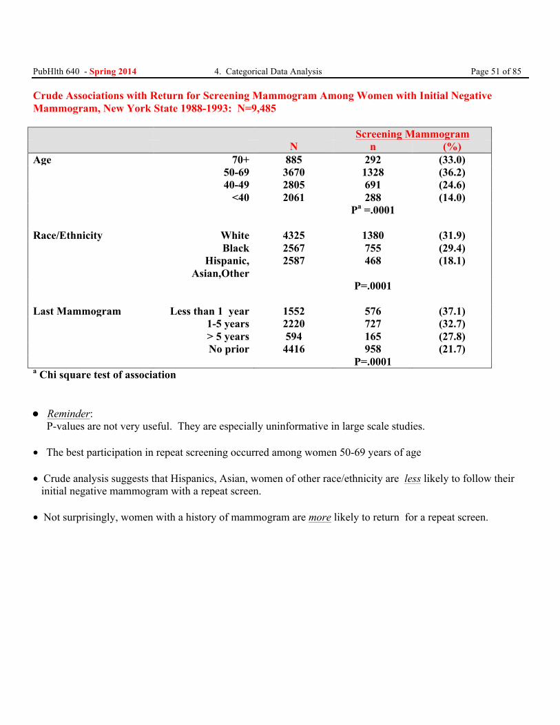
PubHlth 640 - Spring 2014 4. Categorical Data Analysis Page 51 of 85 Crude Associations with Return for Screening Mammogram Among Women with Initial Negative Mammogram, New York State 1988-1993: N=9,485 Screening Mammogram N n (%) Age 70+ 885 292 (33.0) 50-69 3670 1328 (36.2) 40-49 2805 691 (24.6) <40 2061 288 (14.0) Pa =.0001 Race/Ethnicity White 4325 1380 (31.9) Black 2567 755 (29.4) Hispanic,
Asian,Other 2587 468 (18.1)
P=.0001 Last Mammogram Less than 1 year 1552 576 (37.1) 1-5 years 2220 727 (32.7) > 5 years 594 165 (27.8) No prior 4416 958 (21.7) P=.0001 a Chi square test of association • Reminder: P-values are not very useful. They are especially uninformative in large scale studies. • The best participation in repeat screening occurred among women 50-69 years of age • Crude analysis suggests that Hispanics, Asian, women of other race/ethnicity are less likely to follow their initial negative mammogram with a repeat screen. • Not surprisingly, women with a history of mammogram are more likely to return for a repeat screen.
PubHlth 640 - Spring 2014 4. Categorical Data Analysis Page 52 of 85
11. The Chi Square Goodness of Fit Test
Another use of the chi square distribution!
• So far, we’ve used the chi square statistic to test the hypothesis of no association.
• Now we’ll use the chi square distribution to assess whether two distributions are the same or “reasonably” the same (“goodness-of-fit”).
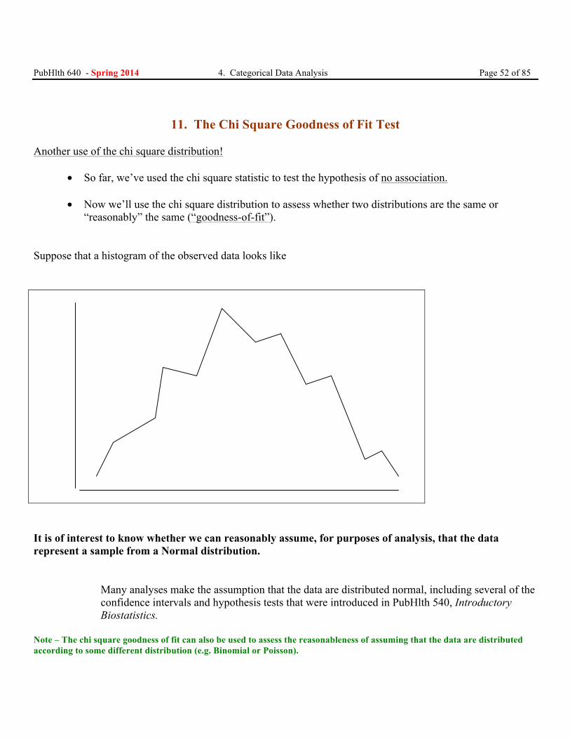
Suppose that a histogram of the observed data looks like
It is of interest to know whether we can reasonably assume, for purposes of analysis, that the data represent a sample from a Normal distribution.
Many analyses make the assumption that the data are distributed normal, including several of the confidence intervals and hypothesis tests that were introduced in PubHlth 540, Introductory Biostatistics.
Note – The chi square goodness of fit can also be used to assess the reasonableness of assuming that the data are distributed according to some different distribution (e.g. Binomial or Poisson).
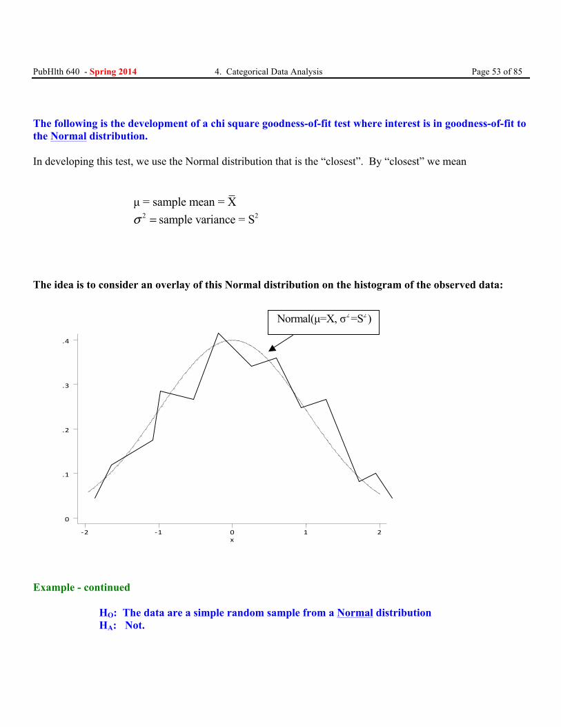
PubHlth 640 - Spring 2014 4. Categorical Data Analysis Page 53 of 85 The following is the development of a chi square goodness-of-fit test where interest is in goodness-of-fit to the Normal distribution. In developing this test, we use the Normal distribution that is the “closest”. By “closest” we mean
µ = sample mean = X 2 2sample variance = Sσ =
The idea is to consider an overlay of this Normal distribution on the histogram of the observed data:
x-‐2 -‐1 0 1 2
0
.1
.2
.3
.4
Example - continued
HO: The data are a simple random sample from a Normal distribution HA: Not.
2 2Normal(µ=X, σ =S )
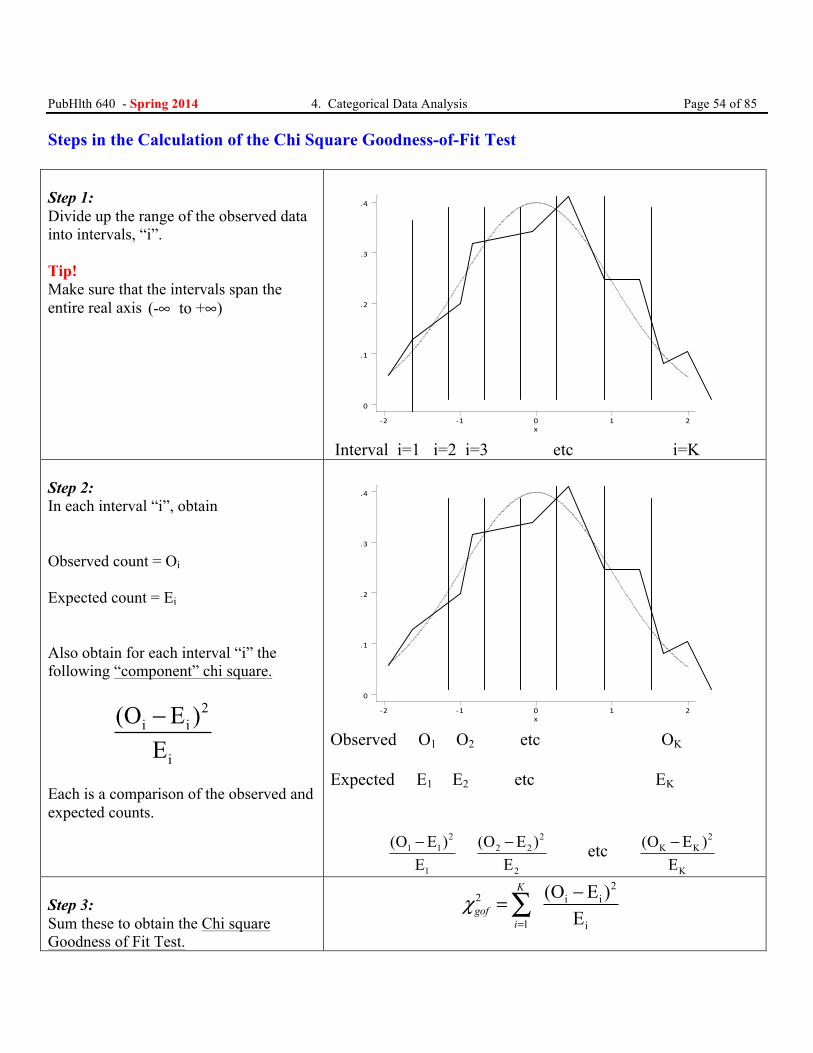
PubHlth 640 - Spring 2014 4. Categorical Data Analysis Page 54 of 85 Steps in the Calculation of the Chi Square Goodness-of-Fit Test Step 1: Divide up the range of the observed data into intervals, “i”. Tip! Make sure that the intervals span the entire real axis (- to + )∞ ∞
x-‐2 -‐1 0 1 2
0
.1
.2
.3
.4
Interval i=1 i=2 i=3 etc i=K
Step 2: In each interval “i”, obtain Observed count = Oi
Expected count = Ei
Also obtain for each interval “i” the following “component” chi square.
2
i i
i
(O E )E−
Each is a comparison of the observed and expected counts.
x-‐2 -‐1 0 1 2
0
.1
.2
.3
.4
Observed O1 O2 etc OK
Expected E1 E2 etc EK
2
1 1
1
(O E )E−
22 2
2
(O E )E− etc
2K K
K
(O E )E−
Step 3: Sum these to obtain the Chi square Goodness of Fit Test.
2
2 i i
1 i
(O E )E
K
gofi
χ=
−=∑
PubHlth 640 - Spring 2014 4. Categorical Data Analysis Page 55 of 85 Example - continued
HO: The data are a simple random sample from a Normal distribution HA: Not.
Behavior of the Chi Square Goodness-of-Fit Statistic
This is a setting where the null hypothesis is typically the one that we hope is operative. The null hypothesis says that the “unknown true” (the distribution that gave rise to the data) is reasonably similar to the hypothesized (in this example, Normal). Values of the chi square goodness of fit test will be small when the two distributions are reasonably similar. This is because the observed and expected counts are similar, giving rise to component chi square values that are small.
How many degrees of freedom does this statistic have? Degrees of Freedom CHI SQUARE GOF = (# intervals) - (1) - (# parameters estimated using data)
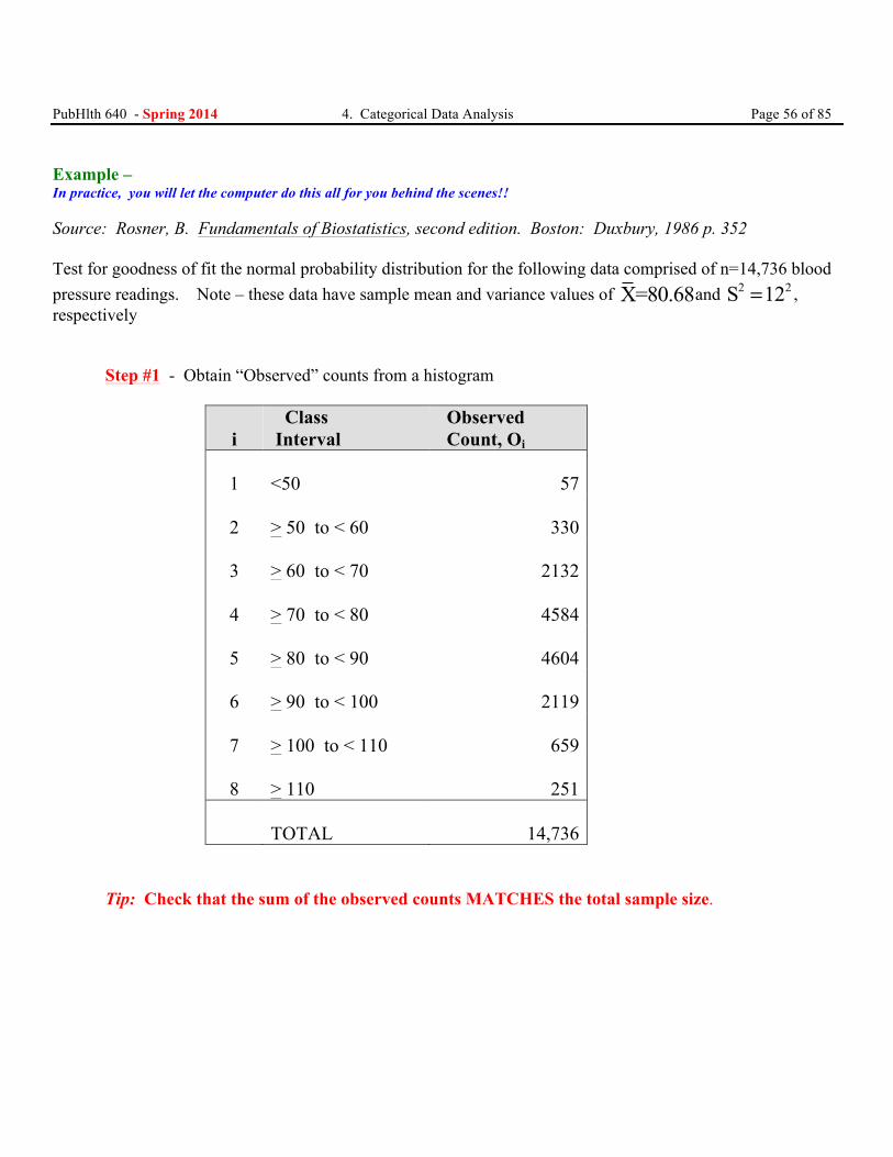
PubHlth 640 - Spring 2014 4. Categorical Data Analysis Page 56 of 85 Example – In practice, you will let the computer do this all for you behind the scenes!! Source: Rosner, B. Fundamentals of Biostatistics, second edition. Boston: Duxbury, 1986 p. 352 Test for goodness of fit the normal probability distribution for the following data comprised of n=14,736 blood pressure readings. Note – these data have sample mean and variance values of X=80.68and 2 2S 12= , respectively
Step #1 - Obtain “Observed” counts from a histogram
i
Class Interval
Observed Count, Oi
1
<50
57
2
> 50 to < 60
330
3
> 60 to < 70
2132
4
> 70 to < 80
4584
5
> 80 to < 90
4604
6
> 90 to < 100
2119
7
> 100 to < 110
659
8
> 110
251
TOTAL
14,736
Tip: Check that the sum of the observed counts MATCHES the total sample size.
PubHlth 640 - Spring 2014 4. Categorical Data Analysis Page 57 of 85
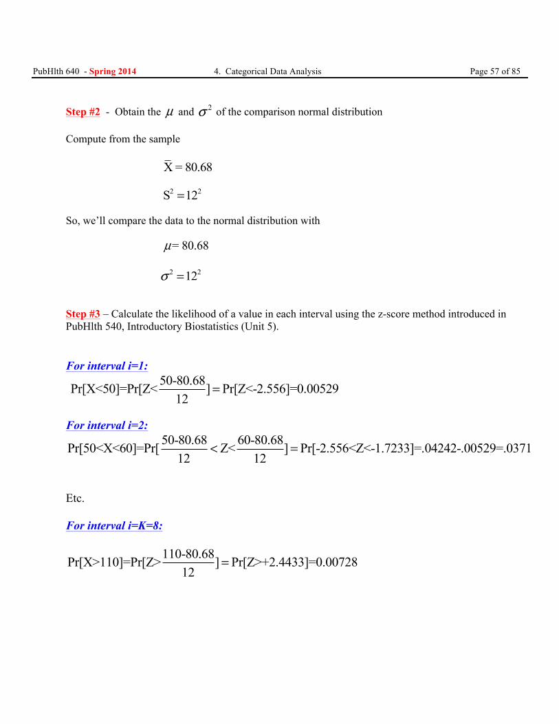
Step #2 - Obtain the µ and 2σ of the comparison normal distribution Compute from the sample
X = 80.68 2 2S 12=
So, we’ll compare the data to the normal distribution with = 80.68µ 2 212σ = Step #3 – Calculate the likelihood of a value in each interval using the z-score method introduced in PubHlth 540, Introductory Biostatistics (Unit 5). For interval i=1:
50-80.68Pr[X<50]=Pr[Z< ] Pr[Z<-2.556]=0.0052912
=
For interval i=2:
50-80.68 60-80.68Pr[50<X<60]=Pr[ Z< ] Pr[-2.556<Z<-1.7233]=.04242-.00529=.037112 12
< =
Etc. For interval i=K=8:
110-80.68Pr[X>110]=Pr[Z> ] Pr[Z>+2.4433]=0.0072812
=
PubHlth 640 - Spring 2014 4. Categorical Data Analysis Page 58 of 85
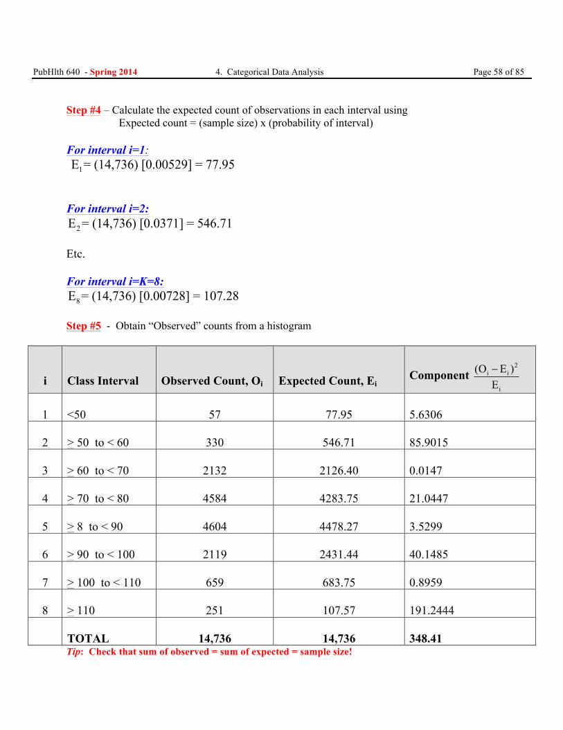
Step #4 – Calculate the expected count of observations in each interval using Expected count = (sample size) x (probability of interval) For interval i=1: 1E = (14,736) [0.00529] = 77.95 For interval i=2:
2E = (14,736) [0.0371] = 546.71 Etc. For interval i=K=8:
8E = (14,736) [0.00728] = 107.28 Step #5 - Obtain “Observed” counts from a histogram
i
Class Interval
Observed Count, Oi
Expected Count, Ei
Component 2
i i
i
(O E )E−
1
<50
57
77.95
5.6306
2
> 50 to < 60
330
546.71
85.9015
3
> 60 to < 70
2132
2126.40
0.0147
4
> 70 to < 80
4584
4283.75
21.0447
5
> 8 to < 90
4604
4478.27
3.5299
6
> 90 to < 100
2119
2431.44
40.1485
7
> 100 to < 110
659
683.75
0.8959
8
> 110
251
107.57
191.2444
TOTAL
14,736
14,736
348.41
Tip: Check that sum of observed = sum of expected = sample size!
PubHlth 640 - Spring 2014 4. Categorical Data Analysis Page 59 of 85
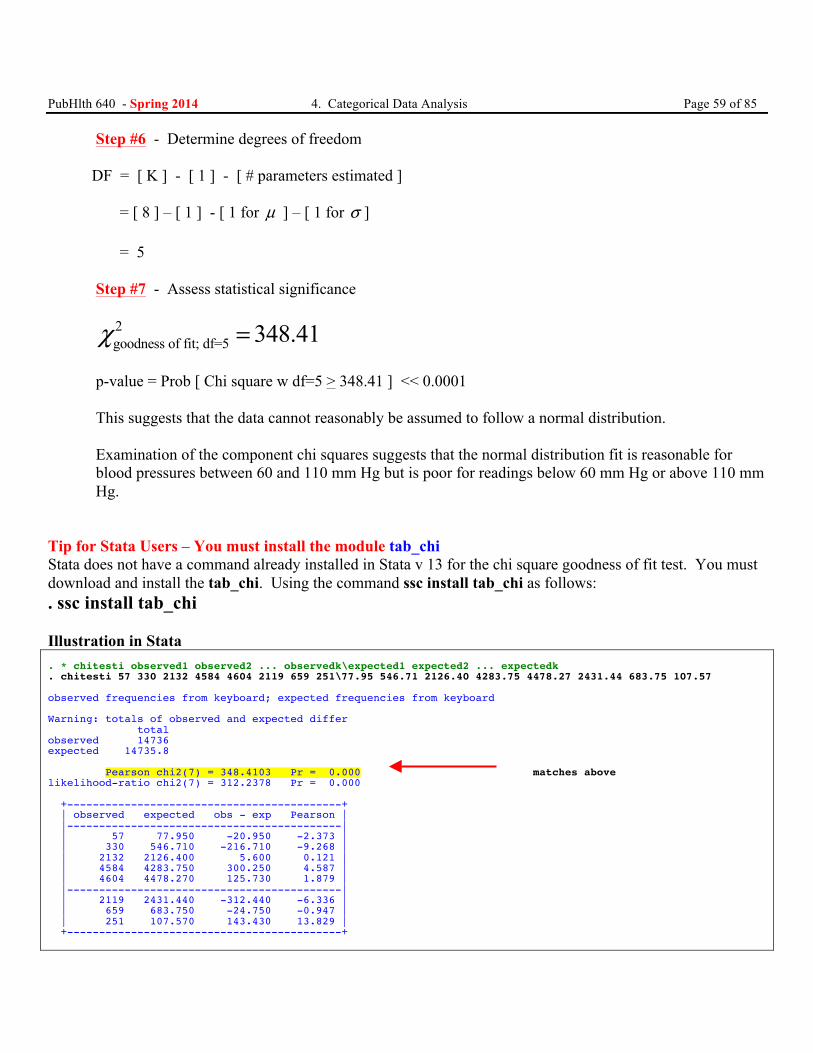
Step #6 - Determine degrees of freedom DF = [ K ] - [ 1 ] - [ # parameters estimated ] = [ 8 ] – [ 1 ] - [ 1 for µ ] – [ 1 for σ ] = 5
Step #7 - Assess statistical significance
2goodness of fit; df=5 348.41χ =
p-value = Prob [ Chi square w df=5 > 348.41 ] << 0.0001 This suggests that the data cannot reasonably be assumed to follow a normal distribution. Examination of the component chi squares suggests that the normal distribution fit is reasonable for blood pressures between 60 and 110 mm Hg but is poor for readings below 60 mm Hg or above 110 mm Hg.
Tip for Stata Users – You must install the module tab_chi Stata does not have a command already installed in Stata v 13 for the chi square goodness of fit test. You must download and install the tab_chi. Using the command ssc install tab_chi as follows: . ssc install tab_chi Illustration in Stata . * chitesti observed1 observed2 ... observedk\expected1 expected2 ... expectedk . chitesti 57 330 2132 4584 4604 2119 659 251\77.95 546.71 2126.40 4283.75 4478.27 2431.44 683.75 107.57 observed frequencies from keyboard; expected frequencies from keyboard Warning: totals of observed and expected differ total observed 14736 expected 14735.8 Pearson chi2(7) = 348.4103 Pr = 0.000 matches above likelihood-ratio chi2(7) = 312.2378 Pr = 0.000 +-------------------------------------------+ | observed expected obs - exp Pearson | |-------------------------------------------| | 57 77.950 -20.950 -2.373 | | 330 546.710 -216.710 -9.268 | | 2132 2126.400 5.600 0.121 | | 4584 4283.750 300.250 4.587 | | 4604 4478.270 125.730 1.879 | |-------------------------------------------| | 2119 2431.440 -312.440 -6.336 | | 659 683.750 -24.750 -0.947 | | 251 107.570 143.430 13.829 | +-------------------------------------------+
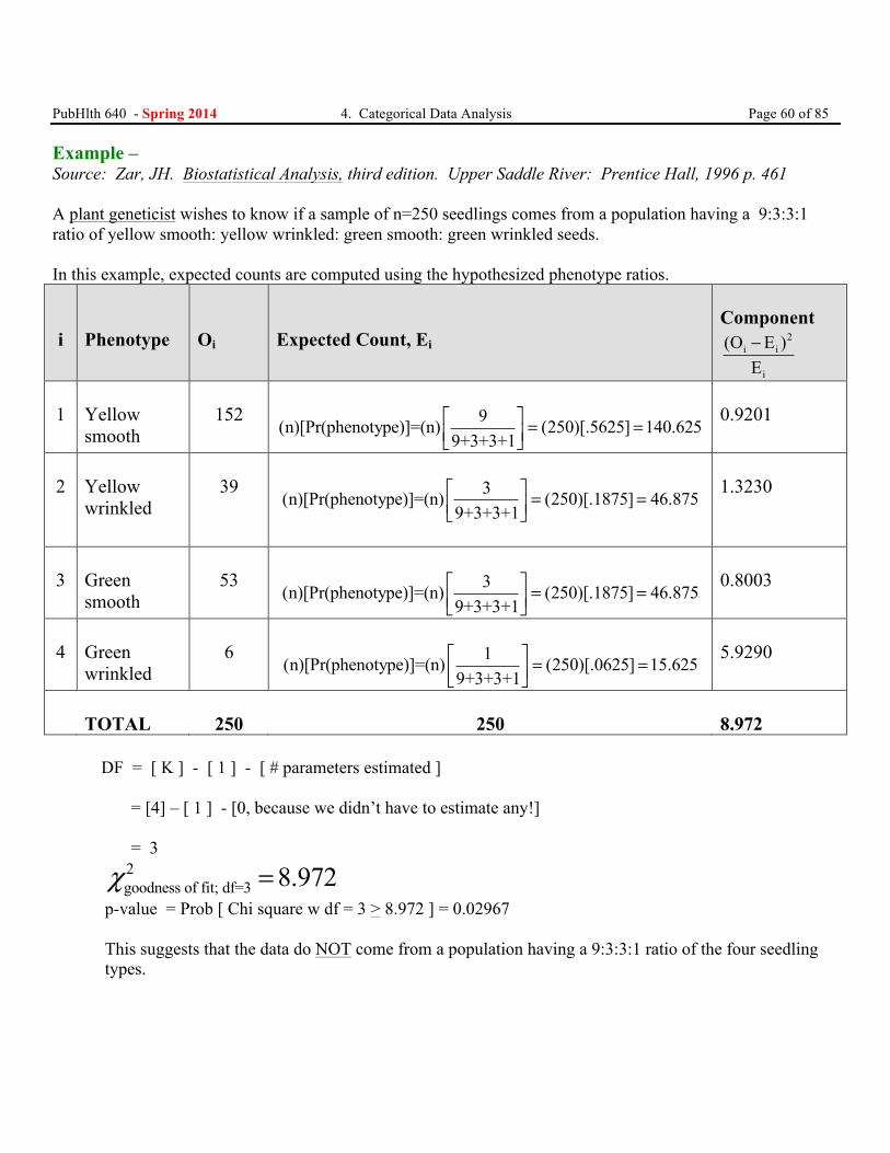
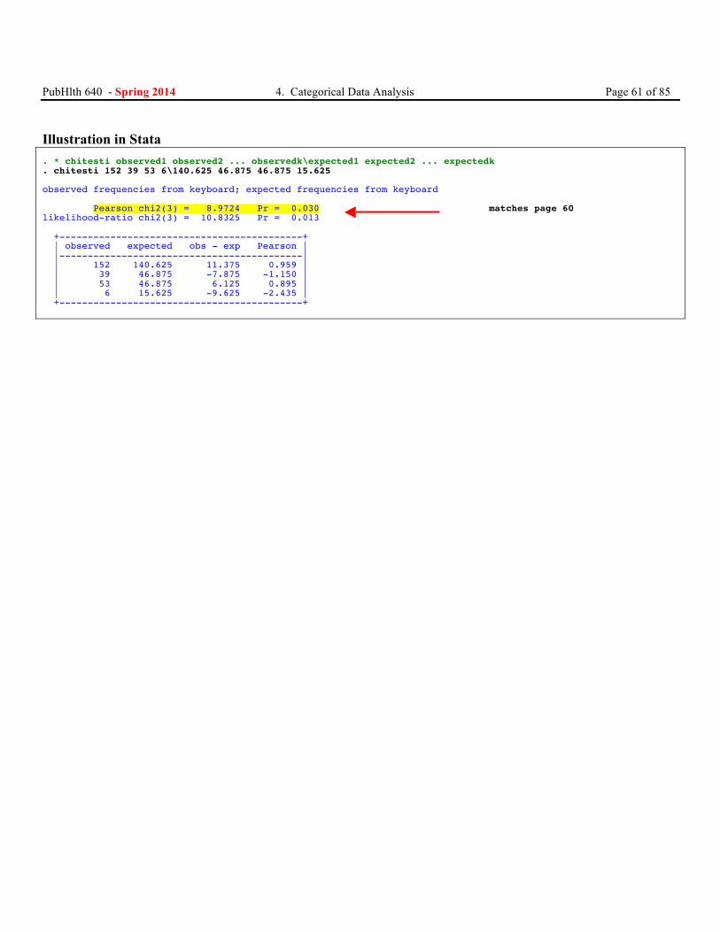
PubHlth 640 - Spring 2014 4. Categorical Data Analysis Page 60 of 85 Example – Source: Zar, JH. Biostatistical Analysis, third edition. Upper Saddle River: Prentice Hall, 1996 p. 461 A plant geneticist wishes to know if a sample of n=250 seedlings comes from a population having a 9:3:3:1 ratio of yellow smooth: yellow wrinkled: green smooth: green wrinkled seeds.
In this example, expected counts are computed using the hypothesized phenotype ratios. i
Phenotype
Oi
Expected Count, Ei
Component
2i i
i
(O E )E−
1
Yellow smooth
152
9(n)[Pr(phenotype)]=(n) (250)[.5625] 140.625
9+3+3+1⎡ ⎤ = =⎢ ⎥⎣ ⎦
0.9201
2
Yellow wrinkled
39
3(n)[Pr(phenotype)]=(n) (250)[.1875] 46.875
9+3+3+1⎡ ⎤ = =⎢ ⎥⎣ ⎦
1.3230
3
Green smooth
53
3(n)[Pr(phenotype)]=(n) (250)[.1875] 46.875
9+3+3+1⎡ ⎤ = =⎢ ⎥⎣ ⎦
0.8003
4
Green wrinkled
6
1(n)[Pr(phenotype)]=(n) (250)[.0625] 15.625
9+3+3+1⎡ ⎤ = =⎢ ⎥⎣ ⎦
5.9290
TOTAL
250
250
8.972
DF = [ K ] - [ 1 ] - [ # parameters estimated ] = [4] – [ 1 ] - [0, because we didn’t have to estimate any!] = 3
2goodness of fit; df=3 8.972χ =
p-value = Prob [ Chi square w df = 3 > 8.972 ] = 0.02967 This suggests that the data do NOT come from a population having a 9:3:3:1 ratio of the four seedling types.
PubHlth 640 - Spring 2014 4. Categorical Data Analysis Page 61 of 85
Illustration in Stata . * chitesti observed1 observed2 ... observedk\expected1 expected2 ... expectedk . chitesti 152 39 53 6\140.625 46.875 46.875 15.625 observed frequencies from keyboard; expected frequencies from keyboard Pearson chi2(3) = 8.9724 Pr = 0.030 matches page 60 likelihood-ratio chi2(3) = 10.8325 Pr = 0.013 +-------------------------------------------+ | observed expected obs - exp Pearson | |-------------------------------------------| | 152 140.625 11.375 0.959 | | 39 46.875 -7.875 -1.150 | | 53 46.875 6.125 0.895 | | 6 15.625 -9.625 -2.435 | +-------------------------------------------+
PubHlth 640 - Spring 2014 4. Categorical Data Analysis Page 62 of 85
Appendix A The Chi Square Distribution
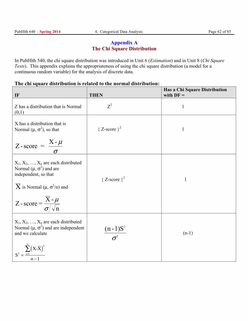
In PubHlth 540, the chi square distribution was introduced in Unit 6 (Estimation) and in Unit 8 (Chi Square Tests). This appendix explains the appropriateness of using the chi square distribution (a model for a continuous random variable) for the analysis of discrete data. The chi square distribution is related to the normal distribution: IF
THEN
Has a Chi Square Distribution with DF =
Z has a distribution that is Normal (0,1)
Z2
1
X has a distribution that is Normal (µ, σ2), so that
Z - score = X -µσ
{ Z-score }2
1
X1, X2, …, Xn are each distributed Normal (µ, σ2) and are independent, so that X is Normal (µ, σ2/n) and
Z - score = X -nµ
σ
{ Z-score }2
1
X1, X2, …, Xn are each distributed Normal (µ, σ2) and are independent and we calculate
S2 =X-X( )2
i=1
n
∑n −1
(n -1)S2
2σ
(n-1)
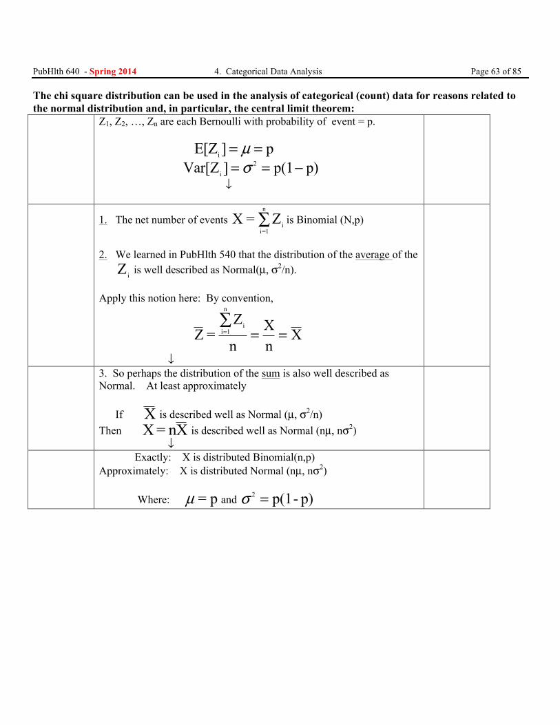
PubHlth 640 - Spring 2014 4. Categorical Data Analysis Page 63 of 85 The chi square distribution can be used in the analysis of categorical (count) data for reasons related to the normal distribution and, in particular, the central limit theorem:
Z1, Z2, …, Zn are each Bernoulli with probability of event = p. E[Z pi ] = =µ
Var[Z ] p(1 p)i2= = −σ
↓
1. The net number of events X = Zi
i=1
n
∑ is Binomial (N,p)
2. We learned in PubHlth 540 that the distribution of the average of the Zi
is well described as Normal(µ, σ2/n). Apply this notion here: By convention,
Z =Z
nXn
Xi
i 1
n
=∑
= =
↓
3. So perhaps the distribution of the sum is also well described as Normal. At least approximately If X is described well as Normal (µ, σ2/n) Then X= nX is described well as Normal (nµ, nσ2) ↓
Exactly: X is distributed Binomial(n,p) Approximately: X is distributed Normal (nµ, nσ2) Where: µ = p and σ 2 p(1- p)=
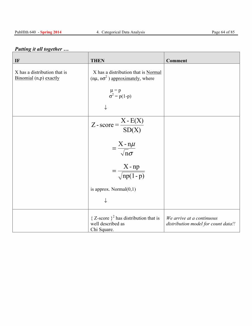
PubHlth 640 - Spring 2014 4. Categorical Data Analysis Page 64 of 85 Putting it all together … IF
THEN
Comment
X has a distribution that is Binomial (n,p) exactly
X has a distribution that is Normal (nµ, nσ2 ) approximately, where µ = p σ2 = p(1-p) ↓
Z - score = X - E(X)
SD(X)
= X - nnµσ
= X - npnp(1- p)
is approx. Normal(0,1) ↓
{ Z-score }2 has distribution that is well described as Chi Square.
We arrive at a continuous distribution model for count data!!
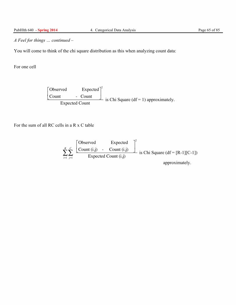
PubHlth 640 - Spring 2014 4. Categorical Data Analysis Page 65 of 85 A Feel for things … continued – You will come to think of the chi square distribution as this when analyzing count data: For one cell
Observed ExpectedCount - Count ⎡
⎣⎢
⎤
⎦⎥
2
Expected Count is Chi Square (df = 1) approximately.
For the sum of all RC cells in a R x C table
j=1
C
∑i=1
R
∑Observed ExpectedCount (i,j) - Count (i,j) ⎡
⎣⎢
⎤
⎦⎥
2
Expected Count (i,j) is Chi Square (df = [R-1][C-1])
approximately.
PubHlth 640 - Spring 2014 4. Categorical Data Analysis Page 66 of 85
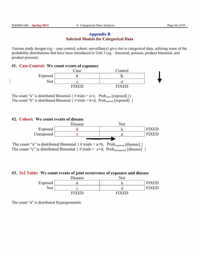
Appendix B Selected Models for Categorical Data
Various study designs (eg – case control, cohort, surveillance) give rise to categorical data, utilizing some of the probability distributions that have been introduced in Unit 3 (eg – binomial, poisson, product binomial, and product poisson).
#1. Case-Control: We count events of exposure Case Control
Exposed a b Not c d
FIXED FIXED The count “a” is distributed Binomial { # trials = a+c, Probcase [exposed] }) The count “b” is distributed Binomial { # trials = b+d, Probcontrol [exposed] }
#2. Cohort: We count events of disease
Disease Not Exposed a b FIXED
Unexposed c d FIXED ⎯⎯ The count “a” is distributed Binomial { # trials = a+b, Probexposed [disease] } The count “c” is distributed Binomial { # trials = c+d, Probunexposed [disease] } #3. 2x2 Table: We count events of joint occurrence of exposure and disease
Disease Not Exposed a b FIXED
Not c d FIXED FIXED FIXED
The count “a” is distributed Hypergeometric
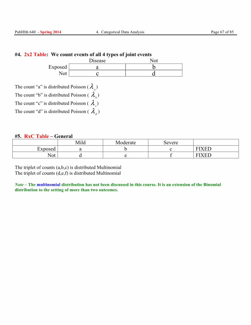
PubHlth 640 - Spring 2014 4. Categorical Data Analysis Page 67 of 85
#4. 2x2 Table: We count events of all 4 types of joint events Disease Not
Exposed a b Not c d
The count “a” is distributed Poisson (λ a )
The count “b” is distributed Poisson ( λ b )
The count “c” is distributed Poisson ( λ c)
The count “d” is distributed Poisson ( λ d )
#5. RxC Table – General Mild Moderate Severe
Exposed a b c FIXED Not d e f FIXED
The triplet of counts (a,b,c) is distributed Multinomial The triplet of counts (d,e,f) is distributed Multinomial
Note – The multinomial distribution has not been discussed in this course. It is an extension of the Binomial distribution to the setting of more than two outcomes.
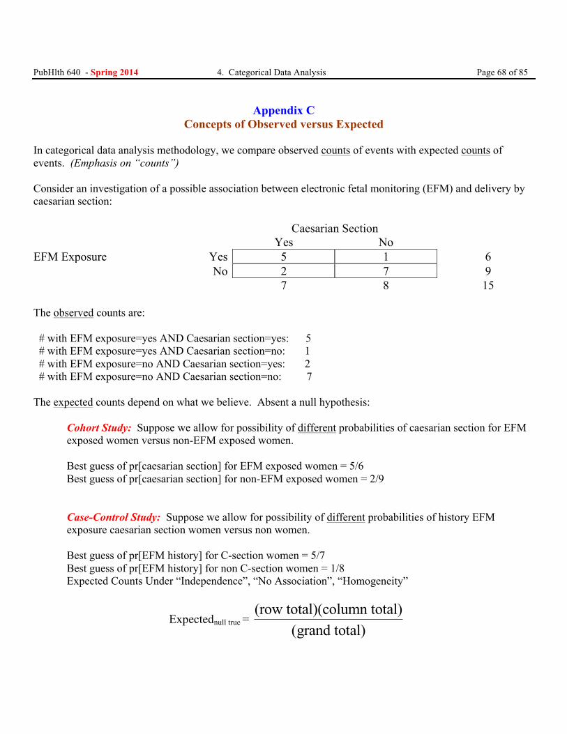
PubHlth 640 - Spring 2014 4. Categorical Data Analysis Page 68 of 85
Appendix C Concepts of Observed versus Expected
In categorical data analysis methodology, we compare observed counts of events with expected counts of events. (Emphasis on “counts”) Consider an investigation of a possible association between electronic fetal monitoring (EFM) and delivery by caesarian section: Caesarian Section Yes No EFM Exposure Yes 5 1 6 No 2 7 9 7 8 15 The observed counts are: # with EFM exposure=yes AND Caesarian section=yes: 5 # with EFM exposure=yes AND Caesarian section=no: 1 # with EFM exposure=no AND Caesarian section=yes: 2 # with EFM exposure=no AND Caesarian section=no: 7 The expected counts depend on what we believe. Absent a null hypothesis:
Cohort Study: Suppose we allow for possibility of different probabilities of caesarian section for EFM exposed women versus non-EFM exposed women. Best guess of pr[caesarian section] for EFM exposed women = 5/6 Best guess of pr[caesarian section] for non-EFM exposed women = 2/9 Case-Control Study: Suppose we allow for possibility of different probabilities of history EFM exposure caesarian section women versus non women. Best guess of pr[EFM history] for C-section women = 5/7 Best guess of pr[EFM history] for non C-section women = 1/8 Expected Counts Under “Independence”, “No Association”, “Homogeneity”
Expectednull true = (row total)(column total)
grand total)(
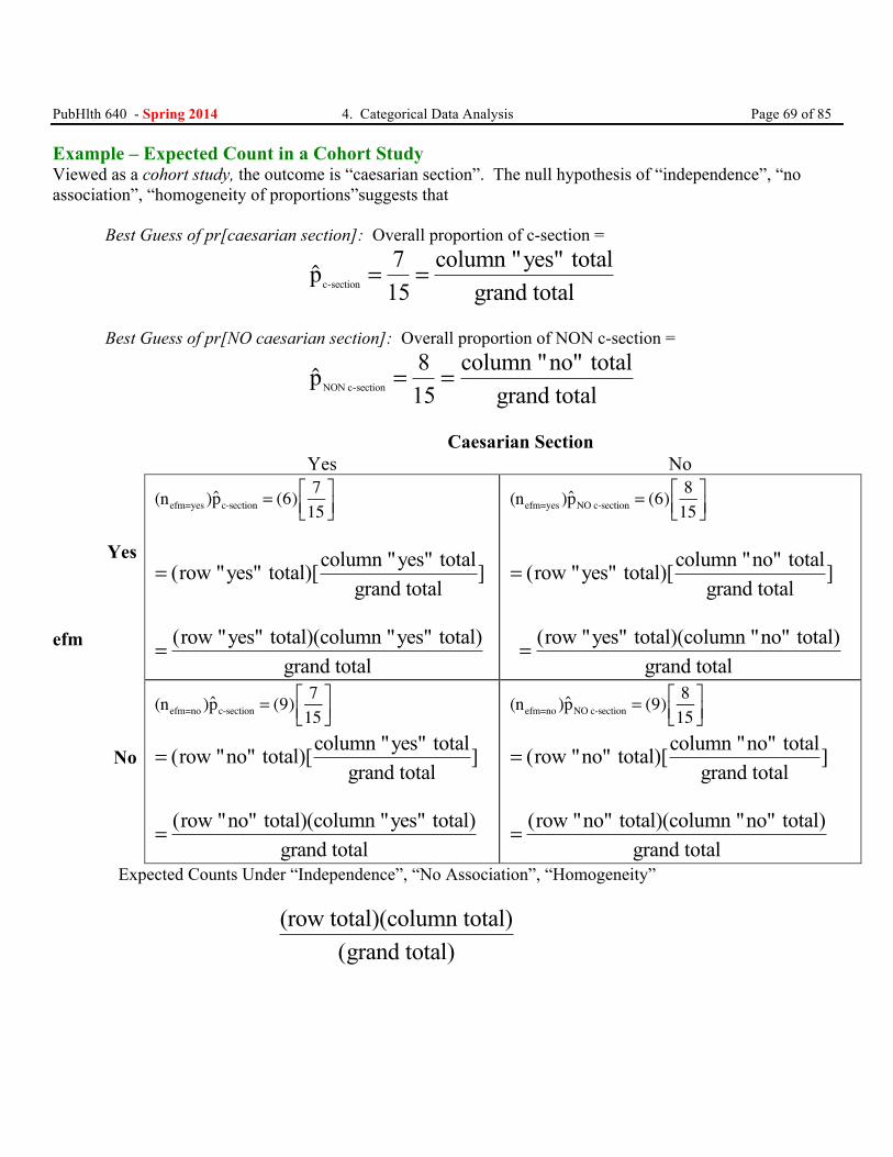
PubHlth 640 - Spring 2014 4. Categorical Data Analysis Page 69 of 85 Example – Expected Count in a Cohort Study Viewed as a cohort study, the outcome is “caesarian section”. The null hypothesis of “independence”, “no association”, “homogeneity of proportions”suggests that
Best Guess of pr[caesarian section]: Overall proportion of c-section =
p column "yes" totalgrand totalc-section = =7
15
Best Guess of pr[NO caesarian section]: Overall proportion of NON c-section =
p column "no" totalgrand totalNON c-section = =8
15
Caesarian Section Yes No efm
Yes
(nefm=yes )p̂c-section = (6)715⎡⎣⎢
⎤⎦⎥
= ( ]row "yes" total)[column "yes" totalgrand total
= (row "yes" total)(column "yes" total)grand total
(nefm=yes )p̂NO c-section = (6) 815⎡⎣⎢
⎤⎦⎥
= ( ]row "yes" total)[column "no" totalgrand total
= (row "yes" total)(column "no" total)grand total
No
(nefm=no )p̂c-section = (9)715⎡⎣⎢
⎤⎦⎥
= ( ]row "no" total)[column "yes" totalgrand total
= (row "no" total)(column "yes" total)grand total
(nefm=no )p̂NO c-section = (9) 815⎡⎣⎢
⎤⎦⎥
= ( ]row "no" total)[column "no" totalgrand total
= (row "no" total)(column "no" total)grand total
Expected Counts Under “Independence”, “No Association”, “Homogeneity”
(row total)(column total)
grand total)(
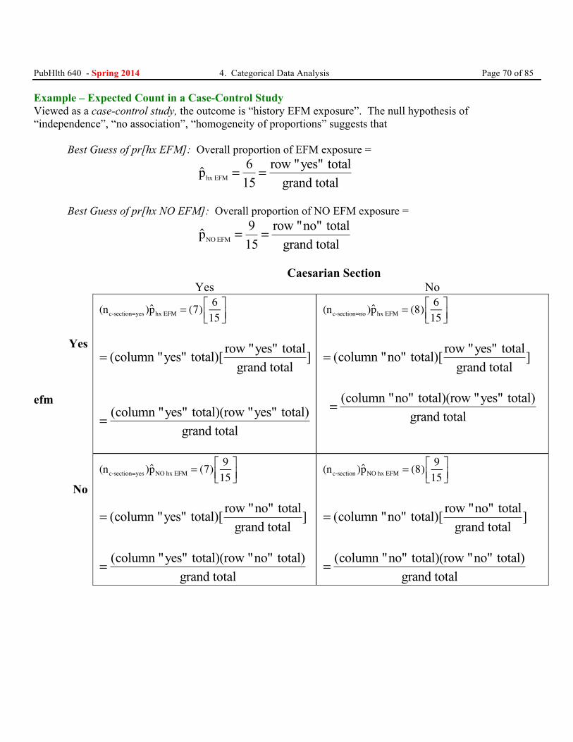
PubHlth 640 - Spring 2014 4. Categorical Data Analysis Page 70 of 85 Example – Expected Count in a Case-Control Study Viewed as a case-control study, the outcome is “history EFM exposure”. The null hypothesis of “independence”, “no association”, “homogeneity of proportions” suggests that
Best Guess of pr[hx EFM]: Overall proportion of EFM exposure =
p row "yes" totalgrand totalhx EFM = =6
15
Best Guess of pr[hx NO EFM]: Overall proportion of NO EFM exposure =
p row "no" totalgrand totalNO EFM = =9
15
Caesarian Section Yes No efm
Yes
(nc-section=yes )p̂hx EFM = (7) 615⎡⎣⎢
⎤⎦⎥
= ( ]column "yes" total)[ row "yes" totalgrand total
= (column "yes" total)(row "yes" total)grand total
(nc-section=no )p̂hx EFM = (8) 615⎡⎣⎢
⎤⎦⎥
= ( ]column "no" total)[ row "yes" totalgrand total
= (column "no" total)(row "yes" total)grand total
No
(nc-section=yes )p̂NO hx EFM = (7) 915⎡⎣⎢
⎤⎦⎥
= ( ]column "yes" total)[ row "no" totalgrand total
= (column "yes" total)(row "no" total)grand total
(nc-section )p̂NO hx EFM = (8) 915⎡⎣⎢
⎤⎦⎥
= ( ]column "no" total)[ row "no" totalgrand total
= (column "no" total)(row "no" total)grand total
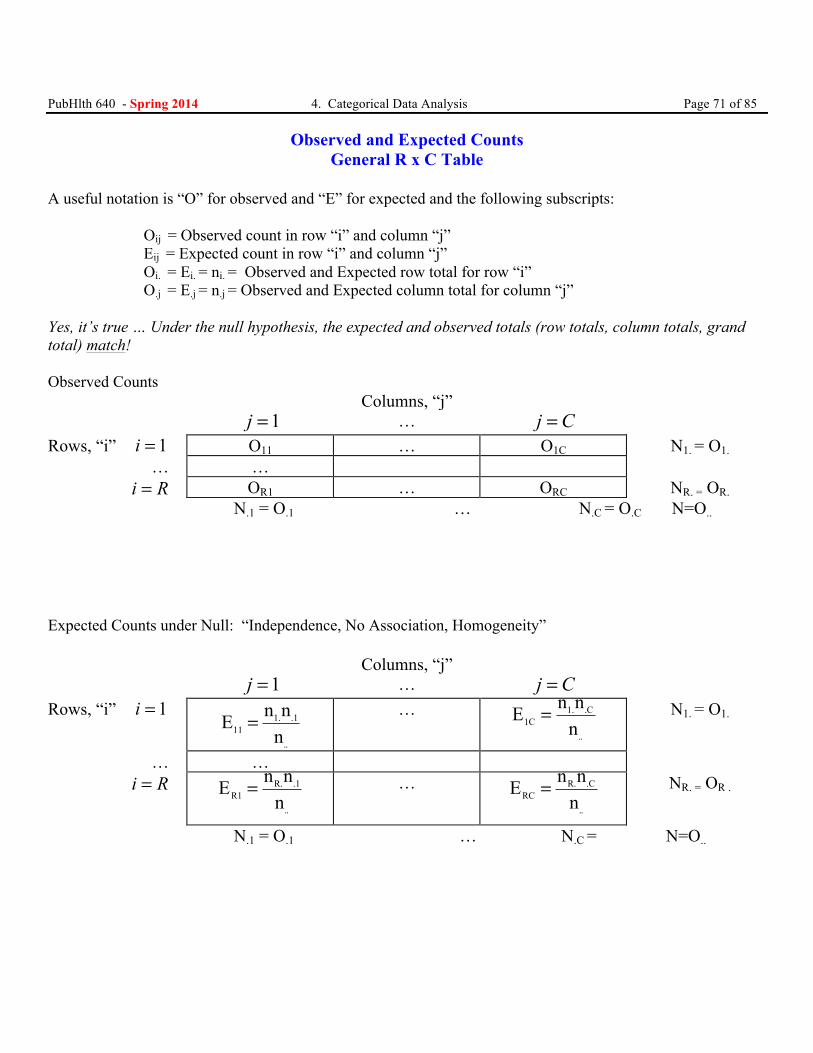
PubHlth 640 - Spring 2014 4. Categorical Data Analysis Page 71 of 85
Observed and Expected Counts General R x C Table
A useful notation is “O” for observed and “E” for expected and the following subscripts: Oij = Observed count in row “i” and column “j” Eij = Expected count in row “i” and column “j” Oi. = Ei. = ni. = Observed and Expected row total for row “i” O.j = E.j = n.j = Observed and Expected column total for column “j” Yes, it’s true … Under the null hypothesis, the expected and observed totals (row totals, column totals, grand total) match! Observed Counts Columns, “j” j =1 … j C= Rows, “i” i = 1 O11 … O1C N1. = O1.
… … i R= OR1 … ORC NR. = OR. N.1 = O.1 … N.C = O.C N=O..
Expected Counts under Null: “Independence, No Association, Homogeneity” Columns, “j” j =1 … j C= Rows, “i” i = 1
E n nn111. .1
..
= … E n n
n1C1. .C
..
= N1. = O1.
… … i R= E n n
nR1R. .1
..
= … E n n
nRCR. .C
..
= NR. = OR .
N.1 = O.1 … N.C = N=O..
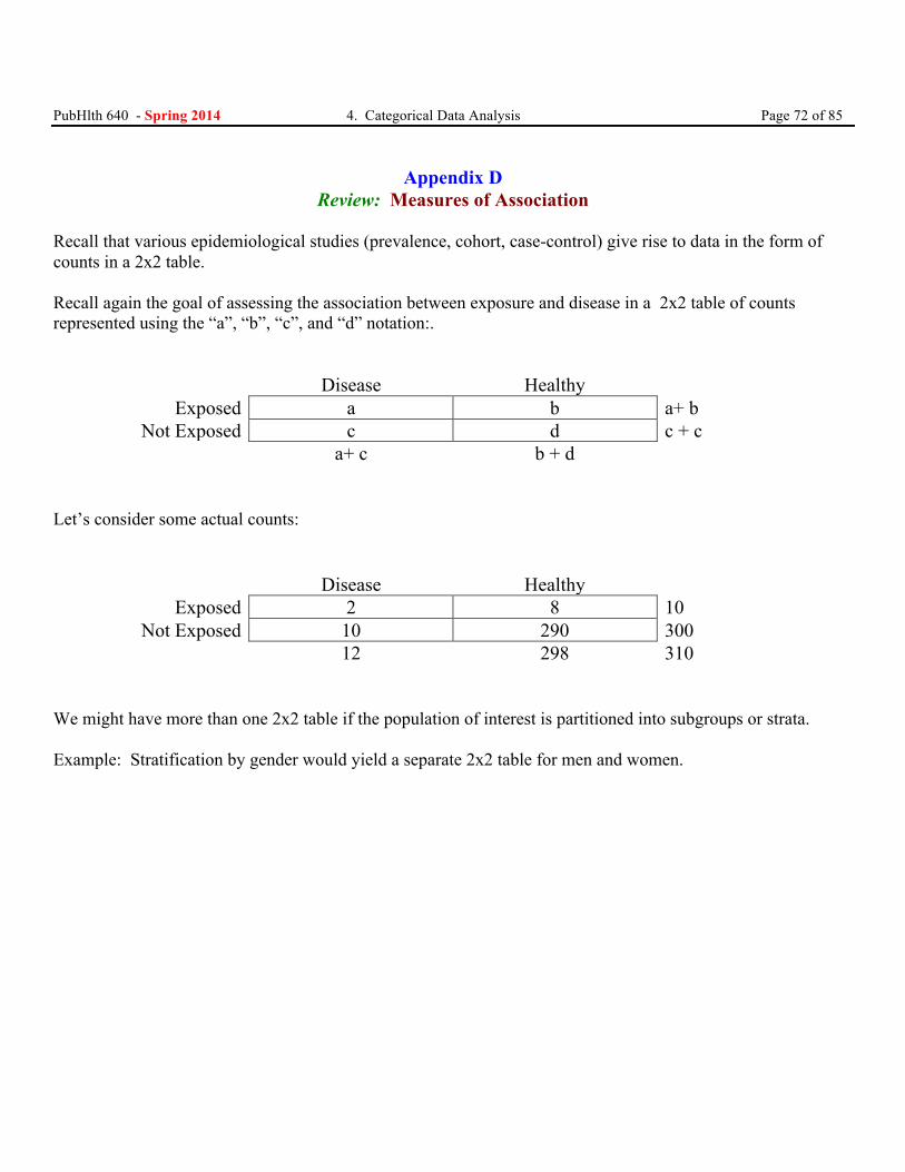
PubHlth 640 - Spring 2014 4. Categorical Data Analysis Page 72 of 85
Appendix D
Review: Measures of Association Recall that various epidemiological studies (prevalence, cohort, case-control) give rise to data in the form of counts in a 2x2 table. Recall again the goal of assessing the association between exposure and disease in a 2x2 table of counts represented using the “a”, “b”, “c”, and “d” notation:.
Disease Healthy Exposed a b a+ b
Not Exposed c d c + c a+ c b + d
Let’s consider some actual counts:
Disease Healthy Exposed 2 8 10
Not Exposed 10 290 300 12 298 310
We might have more than one 2x2 table if the population of interest is partitioned into subgroups or strata. Example: Stratification by gender would yield a separate 2x2 table for men and women.
PubHlth 640 - Spring 2014 4. Categorical Data Analysis Page 73 of 85 A good measure of association is a single measure that is stable over the various characteristics (strata) of the population. Excess Risk Suppose that the cumulative incidence of disease among exposed = π1 and that the cumulative incidence of disease among non-exposed = π0 Excess Risk: The difference between the cumulative incidence rates b = ( π1 - π0 ) Example: In our 2x2 table, we have π1 = 2/10 = .20, π0 = 10/300 = .0333 Thus, b = (.20 - .0333) = .1667 • The effect of exposure is said to be additive because we can write π1 = π0 + b • Hypothesis testing focuses on HO: b = 0 • For a population that has been stratified with strata k = 1 … K, the additive model says that πk1 = πk0 + b Note: The absence of a subscript “k” on the excess risk b says that we are assuming that the excess risk is constant in every stratum (e.g. among men and women). • Biological mechanisms which relate exposure to disease in an additive model often do not operate in the same way across strata. • If so, the additive risk model does not satisfy our criterion of being stable.
PubHlth 640 - Spring 2014 4. Categorical Data Analysis Page 74 of 85 Relative Risk (RR) The relative risk is the ratio of the cumulative incidence rate of disease among the exposed, π1 , to the cumulative incidence rate of disease among the non-exposed, π0. Relative Risk: The ratio of the cumulative incidence rates RR = π1 / π0 Example: In our 2x2 table, we have π1 = 2/10 = .20, π0 = 10/300 = .0333 Thus, RR = .20 / .0333 = 6.006 • The effect of exposure is said to be multiplicative because we can write π1 = [ π0 ] RR • Hypothesis testing focuses on HO: RR = 1 • This model is also said to be additive on the log scale. It is also said to be an example of a log-linear model. To see this: π1 = π0 RR ⇒ ln [ π1 ] = ln [ π0 ] + ln [ RR ] ⇒ ln [ π1 ] = ln [ π0 ] + β where β = ln [ RR ]. • It has been found empirically that many exposure-disease relationships vary with age in such a way that the log linear model is a good description. Specifically, the change with age in the relative risk of disease with exposure is reasonably stable. In such instances, the model is preferable to the additive risk model.
PubHlth 640 - Spring 2014 4. Categorical Data Analysis Page 75 of 85 Attributable Risk The attributable risk is proportion of the incidence of disease among exposed persons that is in excess of the incidence of cases of disease among non-exposed persons. Often, it is expressed as a percent. Attributable Risk:
AR = π ππ1 0
1
− when expressed as a percent.
Recalling that RR = π1 / π0 reveals that
AR = RRRR−1
Example: In our 2x2 table, a RR = 6.006 yields an attributable risk value of AR = (6.006 – 1) / 6.006 = .8335 = 83.35%
PubHlth 640 - Spring 2014 4. Categorical Data Analysis Page 76 of 85 Odds Ratio Recall that the odds ratio measure of association has some wonderful advantages, both biological and analytical. Recall first the meaning of an “odds”: * Probability[event] = π * Odds[Event] = π/(1- π) Let’s look at the odds that are possible in our 2x2 table:
Disease Healthy Exposed a b a+ b
Not Exposed c d c + d a+ c b + d
Cohort study design:
Estimated Odds of disease among exposed = a / (a + b)b / (a + b)⎡⎣⎢
⎤⎦⎥= ab= 28= .25
Estimated Odds of disease among non exposed = c / (c + d)d / (c + d)
⎡⎣⎢
⎤⎦⎥= cd= 10290
= .0345
Case-control study design
Estimated Odds of exposure among diseased = a / (a + c)c / (a + c)
⎡⎣⎢
⎤⎦⎥= ac= 210
= .20
Estimated Odds of exposure among healthy = b / (b + d)d / (b + d)
⎡⎣⎢
⎤⎦⎥= bd= 8290
= .0276
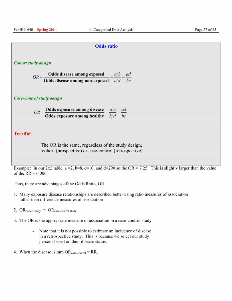
PubHlth 640 - Spring 2014 4. Categorical Data Analysis Page 77 of 85 Odds ratio Cohort study design
Odds disease among exposedOdds disease among non-exposed
a b adORc d bc
= = =
Case-control study design
Odds exposure among diseaseOdds exposure among healthy
a c adORb d bc
= = =
Terrific! The OR is the same, regardless of the study design, cohort (prospective) or case-control (retrospective) Example: In our 2x2 table, a =2, b=8, c=10, and d=290 so the OR = 7.25. This is slightly larger than the value of the RR = 6.006. Thus, there are advantages of the Odds Ratio, OR. 1. Many exposure disease relationships are described better using ratio measures of association rather than difference measures of association 2. ORcohort study = ORcase-control study 3. The OR is the appropriate measure of association in a case-control study.
- Note that it is not possible to estimate an incidence of disease in a retrospective study. This is because we select our study persons based on their disease status.
4. When the disease is rare ORcase-control = RR.
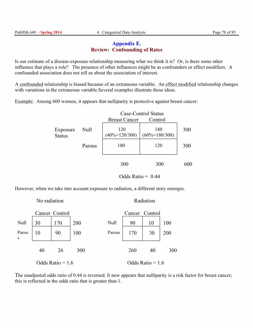
PubHlth 640 - Spring 2014 4. Categorical Data Analysis Page 78 of 85
Appendix E. Review: Confounding of Rates
Is our estimate of a disease-exposure relationship measuring what we think it is? Or, is there some other influence that plays a role? The presence of other influences might be as confounders or effect modifiers. A confounded association does not tell us about the association of interest. A confounded relationship is biased because of an extraneous variable. An effect modified relationship changes with variations in the extraneous variable.Several examples illustrate these ideas. Example: Among 600 women, it appears that nulliparity is protective against breast cancer:
Case-Control Status Breast Cancer Control
Exposure Status
Null
120 (40%=120/300)
180 (60%=180/300)
300
Parous
180
120
300
300 300 600
Odds Ratio = 0.44
However, when we take into account exposure to radiation, a different story emerges.
No radiation Radiation
Cancer Control Cancer Control Null
30
170
200
Null
90
10
100
Parous
10
90
100
Parous
170
30
200
40 26 300 260 40 300 Odds Ratio = 1.6 Odds Ratio = 1.6 The unadjusted odds ratio of 0.44 is reversed. It now appears that nulliparity is a risk factor for breast cancer; this is reflected in the odds ratio that is greater than 1.
PubHlth 640 - Spring 2014 4. Categorical Data Analysis Page 79 of 85 How did this apparent contradiction occur? • In the nulliparous group, there are disproportionately fewer women exposed to radiation. • Women exposed to radiation are more likely to have breast cancer. • Women exposed to radiation were less likely to be nulliparous with the result that • OR = 0.44 is biased due to the confounding effect of exposure to radiation. The calculation of an association (for example an RR or an OR) for a 2x2 table of counts may be misleading because of one or more extraneous influences. An extraneous influence can be
§ Confounder § Effect modifier § Both § Neither
A confounded association is biased and does not tell us about the association of interest. An effect modified relationship changes with variations in the extraneous variable. Intuitively, confounding is the • Distortion of a predictor-outcome relationship due to a third variable that is related to both
- predictor, and - outcome
• The bias from confounding can be a spurious
- strengthening - weakening - elimination - reversal
• A reversal is said to be an example of Simpson’s Paradox
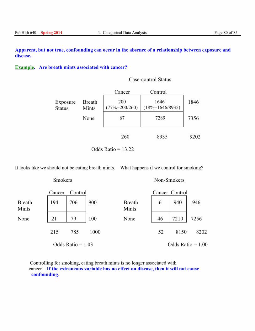
PubHlth 640 - Spring 2014 4. Categorical Data Analysis Page 80 of 85 Apparent, but not true, confounding can occur in the absence of a relationship between exposure and disease.
Example. Are breath mints associated with cancer?
Case-control Status
Cancer Control
Exposure Status
Breath Mints
200 (77%=200/260)
1646 (18%=1646/8935)
1846
None
67
7289
7356
260 8935 9202
Odds Ratio = 13.22 It looks like we should not be eating breath mints. What happens if we control for smoking?
Smokers Non-Smokers
Cancer Control Cancer Control Breath Mints
194
706
900
Breath Mints
6
940
946
None
21
79
100
None
46
7210
7256
215 785 1000 52 8150 8202
Odds Ratio = 1.03 Odds Ratio = 1.00
Controlling for smoking, eating breath mints is no longer associated with cancer. If the extraneous variable has no effect on disease, then it will not cause
confounding.
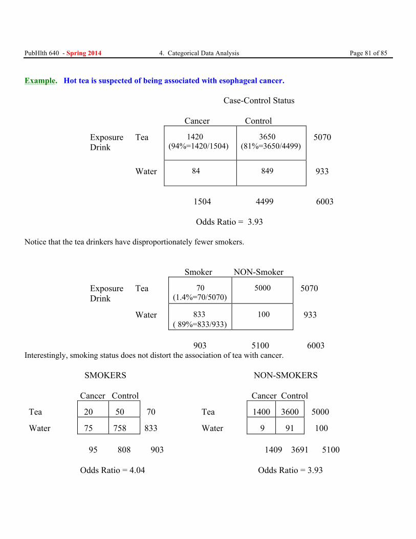
PubHlth 640 - Spring 2014 4. Categorical Data Analysis Page 81 of 85 Example. Hot tea is suspected of being associated with esophageal cancer.
Case-Control Status
Cancer Control
Exposure Drink
Tea
1420 (94%=1420/1504)
3650 (81%=3650/4499)
5070
Water
84
849
933
1504 4499 6003
Odds Ratio = 3.93
Notice that the tea drinkers have disproportionately fewer smokers.
Smoker NON-Smoker
Exposure Drink
Tea
70 (1.4%=70/5070)
5000
5070
Water
833 ( 89%=833/933)
100
933
903 5100 6003
Interestingly, smoking status does not distort the association of tea with cancer.
SMOKERS NON-SMOKERS
Cancer Control Cancer Control Tea
20
50
70
Tea
1400
3600
5000
Water
75
758
833
Water
9
91
100
95 808 903 1409 3691 5100
Odds Ratio = 4.04 Odds Ratio = 3.93
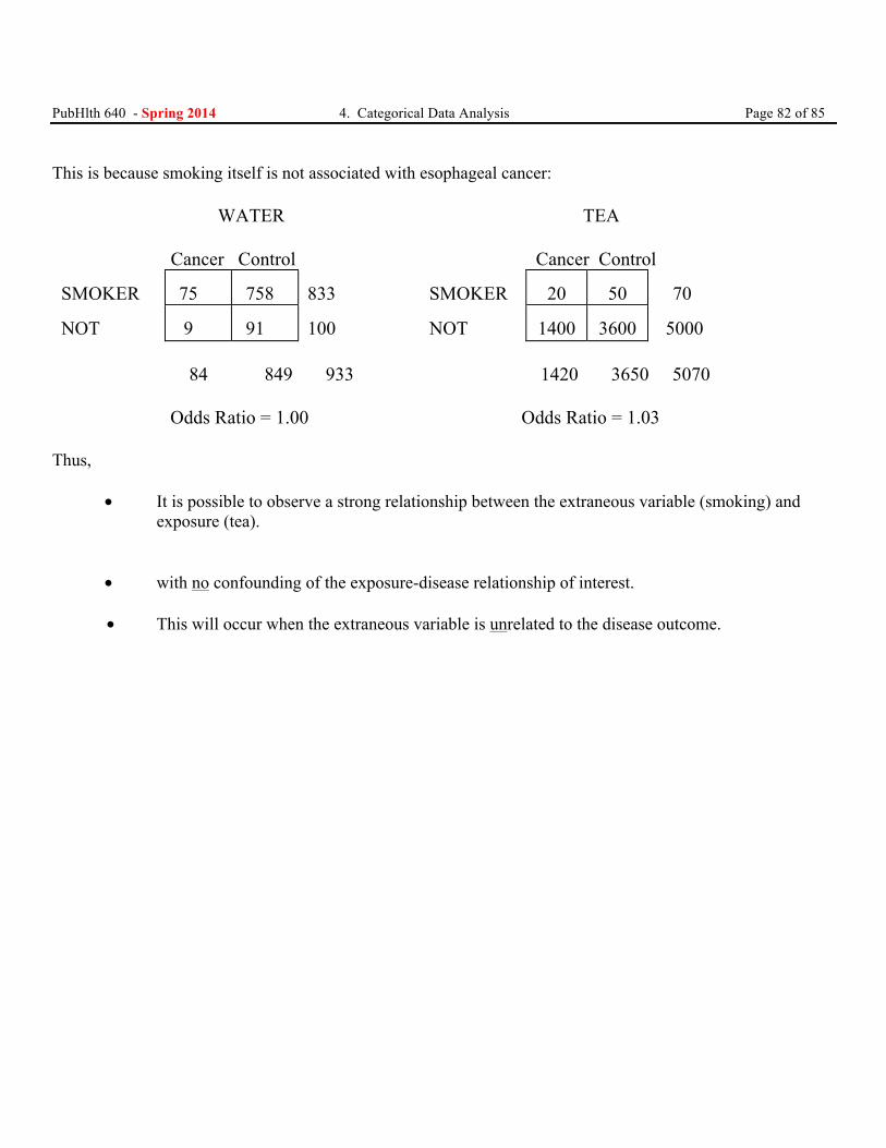
PubHlth 640 - Spring 2014 4. Categorical Data Analysis Page 82 of 85 This is because smoking itself is not associated with esophageal cancer:
WATER TEA
Cancer Control Cancer Control SMOKER
75
758
833
SMOKER
20
50
70
NOT
9
91
100
NOT
1400
3600
5000
84 849 933 1420 3650 5070
Odds Ratio = 1.00 Odds Ratio = 1.03 Thus,
• It is possible to observe a strong relationship between the extraneous variable (smoking) and exposure (tea).
• with no confounding of the exposure-disease relationship of interest.
• This will occur when the extraneous variable is unrelated to the disease outcome.
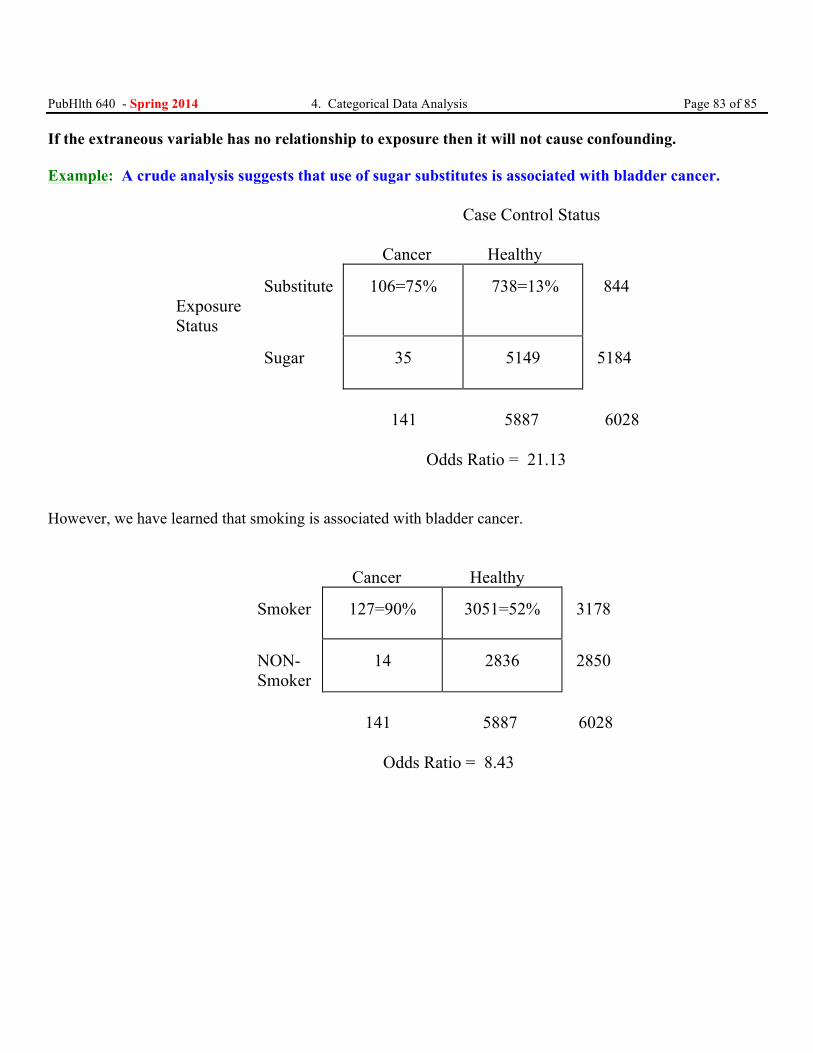
PubHlth 640 - Spring 2014 4. Categorical Data Analysis Page 83 of 85 If the extraneous variable has no relationship to exposure then it will not cause confounding. Example: A crude analysis suggests that use of sugar substitutes is associated with bladder cancer.
Case Control Status
Cancer Healthy
Exposure Status
Substitute
106=75%
738=13%
844
Sugar
35
5149
5184
141 5887 6028
Odds Ratio = 21.13
However, we have learned that smoking is associated with bladder cancer.
Cancer Healthy
Smoker
127=90%
3051=52%
3178
NON-Smoker
14
2836
2850
141 5887 6028
Odds Ratio = 8.43
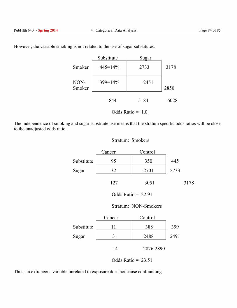
PubHlth 640 - Spring 2014 4. Categorical Data Analysis Page 84 of 85
However, the variable smoking is not related to the use of sugar substitutes.
Substitute Sugar
Smoker
445=14%
2733
3178
NON-Smoker
399=14%
2451
2850
844 5184 6028
Odds Ratio = 1.0
The independence of smoking and sugar substitute use means that the stratum specific odds ratios will be close to the unadjusted odds ratio.
Stratum: Smokers
Cancer Control
Substitute
95
350
445
Sugar
32
2701
2733
127 3051 3178
Odds Ratio = 22.91
Stratum: NON-Smokers
Cancer Control
Substitute
11
388
399
Sugar
3
2488
2491
14 2876 2890
Odds Ratio = 23.51
Thus, an extraneous variable unrelated to exposure does not cause confounding.
PubHlth 640 - Spring 2014 4. Categorical Data Analysis Page 85 of 85 We have what we need to define confounding. Definition Confounding A variable is confounding if
1. It is extraneous, not intermediary
2. It is related to disease, BOTH - among the exposed AND - among the unexposed 3. It is related to exposure.
Recall that an intermediary variable is an intermediate in a causal pathway. - Example: Coal dust → Asthma → Lesions on Lung Asthma is the intermediary variable. - Stratification on an intermediary variable eliminates the exposure disease relationship When we discuss the logistic regression model, we’ll learn about effect modification