4. describing bivariate data - free statistics...
TRANSCRIPT

4. Describing Bivariate Data
A. Introduction to Bivariate Data B. Values of the Pearson CorrelationC. Properties of Pearson's rD. Computing Pearson's rE. Variance Sum Law IIF. Exercises
A dataset with two variables contains what is called bivariate data. This chapter discusses ways to describe the relationship between two variables. For example, you may wish to describe the relationship between the heights and weights of people to determine the extent to which taller people weigh more.
The introductory section gives more examples of bivariate relationships and presents the most common way of portraying these relationships graphically. The next five sections discuss Pearson's correlation, the most common index of the relationship between two variables. The final section, “Variance Sum Law II,” makes use of Pearson's correlation to generalize this law to bivariate data.
164

Introduction to Bivariate Databy Rudy Guerra and David M. Lane
Prerequisites• Chapter 1: Variables• Chapter 1: Distributions• Chapter 2: Histograms• Chapter 3: Measures of Central Tendency• Chapter 3: Variability• Chapter 3: Shapes of Distributions
Learning Objectives1. Define “bivariate data”2. Define “scatter plot”3. Distinguish between a linear and a nonlinear relationship4. Identify positive and negative associations from a scatter plotMeasures of central tendency, variability, and spread summarize a single variable by providing important information about its distribution. Often, more than one variable is collected on each individual. For example, in large health studies of populations it is common to obtain variables such as age, sex, height, weight, blood pressure, and total cholesterol on each individual. Economic studies may be interested in, among other things, personal income and years of education. As a third example, most university admissions committees ask for an applicant's high school grade point average and standardized admission test scores (e.g., SAT). In this chapter we consider bivariate data, which for now consists of two quantitative variables for each individual. Our first interest is in summarizing such data in a way that is analogous to summarizing univariate (single variable) data.
By way of illustration, let's consider something with which we are all familiar: age. Let’s begin by asking if people tend to marry other people of about the same age. Our experience tells us “yes,” but how good is the correspondence? One way to address the question is to look at pairs of ages for a sample of married couples. Table 1 below shows the ages of 10 married couples. Going across the columns we see that, yes, husbands and wives tend to be of about the same age, with men having a tendency to be slightly older than their wives. This is no big
165

surprise, but at least the data bear out our experiences, which is not always the case.
Table 1. Sample of spousal ages of 10 White American Couples.
Husband 36 72 37 36 51 50 47 50 37 41
Wife 35 67 33 35 50 46 47 42 36 41
The pairs of ages in Table 1 are from a dataset consisting of 282 pairs of spousal ages, too many to make sense of from a table. What we need is a way to summarize the 282 pairs of ages. We know that each variable can be summarized by a histogram (see Figure 1) and by a mean and standard deviation (See Table 2).
Figure 1. Histograms of spousal ages.
Table 2. Means and standard deviations of spousal ages.
MeanStandardDeviation
Husbands 49 11
Wives 47 11
Each distribution is fairly skewed with a long right tail. From Table 1 we see that not all husbands are older than their wives and it is important to see that this fact is lost when we separate the variables. That is, even though we provide summary statistics on each variable, the pairing within couple is lost by separating the variables. We cannot say, for example, based on the means alone what percentage of couples has younger husbands than wives. We have to count across pairs to find this out. Only by maintaining the pairing can meaningful answers be found about couples per se. Another example of information not available from the separate descriptions of husbands and wives' ages is the mean age of husbands with wives
166
of a certain age. For instance, what is the average age of husbands with 45-year-old wives? Finally, we do not know the relationship between the husband's age and the wife's age.
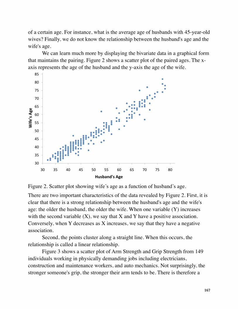
We can learn much more by displaying the bivariate data in a graphical form that maintains the pairing. Figure 2 shows a scatter plot of the paired ages. The x-axis represents the age of the husband and the y-axis the age of the wife.
30
35
40
45
50
55
60
65
70
75
80
85
30 35 40 45 50 55 60 65 70 75 80
Wife
's'Ag
e
Husband's'Age
Figure 2. Scatter plot showing wife’s age as a function of husband’s age.There are two important characteristics of the data revealed by Figure 2. First, it is clear that there is a strong relationship between the husband's age and the wife's age: the older the husband, the older the wife. When one variable (Y) increases with the second variable (X), we say that X and Y have a positive association. Conversely, when Y decreases as X increases, we say that they have a negative association.
Second, the points cluster along a straight line. When this occurs, the relationship is called a linear relationship.
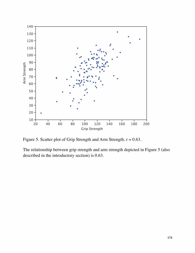
Figure 3 shows a scatter plot of Arm Strength and Grip Strength from 149 individuals working in physically demanding jobs including electricians, construction and maintenance workers, and auto mechanics. Not surprisingly, the stronger someone's grip, the stronger their arm tends to be. There is therefore a
167
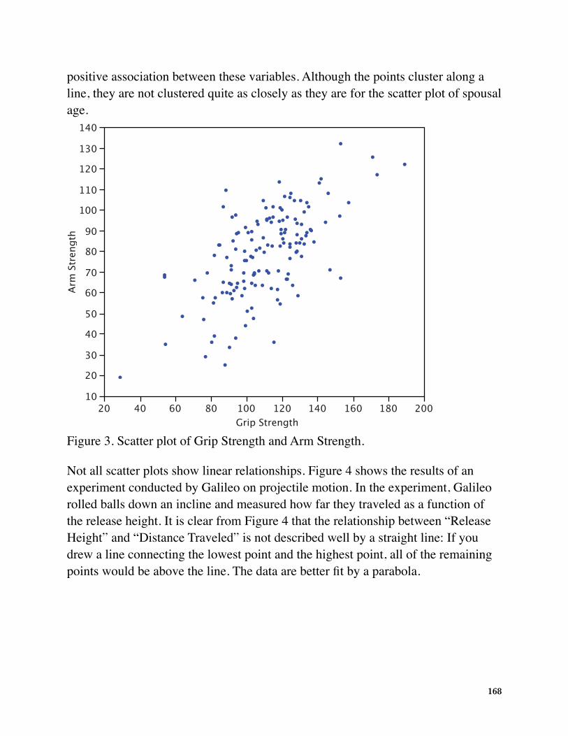
positive association between these variables. Although the points cluster along a line, they are not clustered quite as closely as they are for the scatter plot of spousal age.
10
2030
4050
6070
8090
100110
120130
140
Arm$Strength
20 40 60 80 100 120 140 160 180 200Grip$Strength
Figure 3. Scatter plot of Grip Strength and Arm Strength.
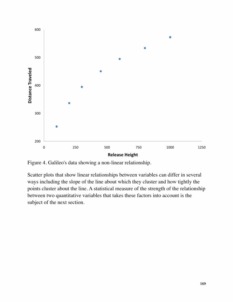
Not all scatter plots show linear relationships. Figure 4 shows the results of an experiment conducted by Galileo on projectile motion. In the experiment, Galileo rolled balls down an incline and measured how far they traveled as a function of the release height. It is clear from Figure 4 that the relationship between “Release Height” and “Distance Traveled” is not described well by a straight line: If you drew a line connecting the lowest point and the highest point, all of the remaining points would be above the line. The data are better fit by a parabola.
168
200
300
400
500
600
0 250 500 750 1000 1250
Distan
ce)Traveled
Release)Height
Figure 4. Galileo's data showing a non-linear relationship.
Scatter plots that show linear relationships between variables can differ in several ways including the slope of the line about which they cluster and how tightly the points cluster about the line. A statistical measure of the strength of the relationship between two quantitative variables that takes these factors into account is the subject of the next section.
169
Values of the Pearson Correlationby David M. Lane
Prerequisites• Chapter 4: Introduction to Bivariate Data
Learning Objectives1. Describe what Pearson's correlation measures2. Give the symbols for Pearson's correlation in the sample and in the population3. State the possible range for Pearson's correlation4. Identify a perfect linear relationshipThe Pearson product-moment correlation coefficient is a measure of the strength of the linear relationship between two variables. It is referred to as Pearson's correlation or simply as the correlation coefficient. If the relationship between the variables is not linear, then the correlation coefficient does not adequately represent the strength of the relationship between the variables.
The symbol for Pearson's correlation is “ρ” when it is measured in the population and “r” when it is measured in a sample. Because we will be dealing almost exclusively with samples, we will use r to represent Pearson's correlation unless otherwise noted.
Pearson's r can range from -1 to 1. An r of -1 indicates a perfect negative linear relationship between variables, an r of 0 indicates no linear relationship between variables, and an r of 1 indicates a perfect positive linear relationship between variables. Figure 1 shows a scatter plot for which r = 1.
170

!6
!5
!4
!3
!2
!1
0
1
2
3
4
!3 !2 !1 0 1 2 3
y
xFigure 1. A perfect linear relationship, r = 1.
171

!6
!4
!2
0
2
4
6
8
!3 !2 !1 0 1 2 3
y
x
Figure 2. A perfect negative linear relationship, r = -1.
!3
!2
!1
0
1
2
3
4
!3 !2 !1 0 1 2 3
y
x
172

Figure 3. A scatter plot for which r = 0. Notice that there is no relationship between X and Y.
With real data, you would not expect to get values of r of exactly -1, 0, or 1. The data for spousal ages shown in Figure 4 and described in the introductory section has an r of 0.97.
30
35
40
45
50
55
60
65
70
75
80
85
30 35 40 45 50 55 60 65 70 75 80
Wife
's'Ag
e
Husband's'Age
Figure 4. Scatter plot of spousal ages, r = 0.97.
173
10
2030
4050
6070
8090
100110
120130
140Arm$Strength
20 40 60 80 100 120 140 160 180 200Grip$Strength
Figure 5. Scatter plot of Grip Strength and Arm Strength, r = 0.63.
The relationship between grip strength and arm strength depicted in Figure 5 (also described in the introductory section) is 0.63.
174
Properties of Pearson's rby David M. Lane
Prerequisites• Chapter 1: Linear Transformations• Chapter 4: Introduction to Bivariate Data
Learning Objectives1. State the range of values for Pearson's correlation2. State the values that represent perfect linear relationships3. State the relationship between the correlation of Y with X and the correlation of
X with Y4. State the effect of linear transformations on Pearson's correlationA basic property of Pearson's r is that its possible range is from -1 to 1. A correlation of -1 means a perfect negative linear relationship, a correlation of 0 means no linear relationship, and a correlation of 1 means a perfect positive linear relationship.
Pearson's correlation is symmetric in the sense that the correlation of X with Y is the same as the correlation of Y with X. For example, the correlation of Weight with Height is the same as the correlation of Height with Weight.
A critical property of Pearson's r is that it is unaffected by linear transformations. This means that multiplying a variable by a constant and/or adding a constant does not change the correlation of that variable with other variables. For instance, the correlation of Weight and Height does not depend on whether Height is measured in inches, feet, or even miles. Similarly, adding five points to every student's test score would not change the correlation of the test score with other variables such as GPA.
175

Computing Pearson's rby David M. Lane
Prerequisites• Chapter 1: Summation Notation• Chapter 4: Introduction to Bivariate Data
Learning Objectives1. Define X and x2. State why Σxy = 0 when there is no relationship3. Calculate rThere are several formulas that can be used to compute Pearson's correlation. Some formulas make more conceptual sense whereas others are easier to actually compute. We are going to begin with a formula that makes more conceptual sense.
We are going to compute the correlation between the variables X and Y shown in Table 1. We begin by computing the mean for X and subtracting this mean from all values of X. The new variable is called “x.” The variable “y” is computed similarly. The variables x and y are said to be deviation scores because each score is a deviation from the mean. Notice that the means of x and y are both 0. Next we create a new column by multiplying x and y.
Before proceeding with the calculations, let's consider why the sum of the xy column reveals the relationship between X and Y. If there were no relationship between X and Y, then positive values of x would be just as likely to be paired with negative values of y as with positive values. This would make negative values of xy as likely as positive values and the sum would be small. On the other hand, consider Table 1 in which high values of X are associated with high values of Y and low values of X are associated with low values of Y. You can see that positive values of x are associated with positive values of y and negative values of x are associated with negative values of y. In all cases, the product of x and y is positive, resulting in a high total for the xy column. Finally, if there were a negative relationship then positive values of x would be associated with negative values of y and negative values of x would be associated with positive values of y. This would lead to negative values for xy.
176

Table 1. Calculation of r. X Y x y xy x2 y2
1 4 -3 -5 15 9 25
3 6 -1 -3 3 1 9
5 10 1 1 1 1 1
5 12 1 3 3 1 9
6 13 2 4 8 4 16
Total 20 45 0 0 30 16 60
Mean 4 9 0 0 6
Pearson's r is designed so that the correlation between height and weight is the same whether height is measured in inches or in feet. To achieve this property, Pearson's correlation is computed by dividing the sum of the xy column (Σxy) by the square root of the product of the sum of the x2 column (Σx2) and the sum of the y2 column (Σy2). The resulting formula is:
Computing Pearson’s r
� =���
��� ��
� =30
�(16)(60)=
30�960
=30
30.984 = 0.968
� =��� � �����
���� � (��)
� ����� � (��)
� �
Variance Sum Law II
��± = �� + �
��± = �� + � ± 2����
������������ = 10,000 + 11,000 + (2)(0.5)�10,000�11,000
������������� = 10,000 + 11,000� (2)(0.5)�10,000�11,000
and therefore
Computing Pearson’s r
� =���
��� ��
� =30
�(16)(60)=
30�960
=30
30.984 = 0.968
� =��� � �����
���� � (��)
� ����� � (��)
� �
Variance Sum Law II
��± = �� + �
��± = �� + � ± 2����
������������ = 10,000 + 11,000 + (2)(0.5)�10,000�11,000
������������� = 10,000 + 11,000� (2)(0.5)�10,000�11,000
An alternative computational formula that avoids the step of computing deviation scores is:
Computing Pearson’s r
� =���
��� ��
� =30
�(16)(60)=
30�960
=30
30.984 = 0.968
� =��� � �����
���� � (��)
� ����� � (��)
� �
Variance Sum Law II
��± = �� + �
��± = �� + � ± 2����
������������ = 10,000 + 11,000 + (2)(0.5)�10,000�11,000
������������� = 10,000 + 11,000� (2)(0.5)�10,000�11,000
177

Variance Sum Law IIby David M. Lane
Prerequisites• Chapter 1: Variance Sum Law I• Chapter 4: Values of Pearson's Correlation
Learning Objectives1. State the variance sum law when X and Y are not assumed to be independent2. Compute the variance of the sum of two variables if the variance of each and
their correlation is known3. Compute the variance of the difference between two variables if the variance of
each and their correlation is knownRecall that when the variables X and Y are independent, the variance of the sum or difference between X and Y can be written as follows:
Computing Pearson’s r
� =���
��� ��
� =30
�(16)(60)=
30�960
=30
30.984 = 0.968
� =��� � �����
���� � (��)
� ����� � (��)
� �
Variance Sum Law II
��± = �� + �
��± = �� + � ± 2����
������������ = 10,000 + 11,000 + (2)(0.5)�10,000�11,000
������������� = 10,000 + 11,000� (2)(0.5)�10,000�11,000
which is read: “The variance of X plus or minus Y is equal to the variance of X plus the variance of Y.”
When X and Y are correlated, the following formula should be used:
Computing Pearson’s r
� =���
��� ��
� =30
�(16)(60)=
30�960
=30
30.984 = 0.968
� =��� � �����
���� � (��)
� ����� � (��)
� �
Variance Sum Law II
��± = �� + �
��± = �� + � ± 2����
������������ = 10,000 + 11,000 + (2)(0.5)�10,000�11,000
������������� = 10,000 + 11,000� (2)(0.5)�10,000�11,000
where ρ is the correlation between X and Y in the population. For example, if the variance of verbal SAT were 10,000, the variance of quantitative SAT were 11,000 and the correlation between these two tests were 0.50, then the variance of total SAT (verbal + quantitative) would be:
Computing Pearson’s r
� =���
��� ��
� =30
�(16)(60)=
30�960
=30
30.984 = 0.968
� =��� � �����
���� � (��)
� ����� � (��)
� �
Variance Sum Law II
��± = �� + �
��± = �� + � ± 2����
������������ = 10,000 + 11,000 + (2)(0.5)�10,000�11,000
������������� = 10,000 + 11,000� (2)(0.5)�10,000�11,000 which is equal to 31,488. The variance of the difference is:
Computing Pearson’s r
� =���
��� ��
� =30
�(16)(60)=
30�960
=30
30.984 = 0.968
� =��� � �����
���� � (��)
� ����� � (��)
� �
Variance Sum Law II
��± = �� + �
��± = �� + � ± 2����
������������ = 10,000 + 11,000 + (2)(0.5)�10,000�11,000
������������� = 10,000 + 11,000� (2)(0.5)�10,000�11,000
178

which is equal to 10,512.If the variances and the correlation are computed in a sample, then the
following notation is used to express the variance sum law:
��±�� = ��� + ��� ± 2�����
179

Statistical Literacyby David M. Lane
Prerequisites• Chapter 4: Values of Pearson's Correlation
The graph below showing the relationship between age and sleep is based on a graph that appears on this web page.
What do you think?Why might Pearson's correlation not be a good way to describe the relationship?
Pearson's correlation measures the strength of the linear relationship between two variables. The relationship here is not linear. As age increases, hours slept decreases rapidly at first but then levels off.
180

Exercises
Prerequisites• All material presented in the Describing Bivariate Data chapter
1. Describe the relationship between variables A and C. Think of things these variables could represent in real life.
�� �������������������������������
5-��� ������!�������"�� ������!&����%������� ��������-����������!���� �!�� ��%������� ���$�������� ��!�������������-�
6-�����$������!�� �!�&�!��54��$���� �!��!��� ����� �"%���������"��-�
7-�����$������!�� �!�&�!��54��$���� �!��!��� �������"%���������"��-�
8-����!����������"�����!&����&����!�0�����$�� 1����������!�0������!1�� �4-9;+����,�0�1�!��������/��"�����!&����&����!�0�����$�� 1����������!�0���(��� 1�0�1�!����������"�����!&����&����!�0����������� 1����������!�0�����!�� 1-4-9;�4-9;������������"���������!��0�1�����0�1�� � "���4-9;�����$ ���������!��� �����"�� ������!�����!�!���%��$�������� ��. ��������"��+�������!�����!������%���� !���� ������������!��� �����"�� -
9-� �$���(�$��'���!�!����������"�����!&����������������������������������!������������&����!����������(�$����"�������� ��������� ����&����!�������������(�!���!���64� !$/���! *� �(*�����������"���&�����������(��������������&�����������!���������!�����"�������� ��������� +�����$ ��!����������� !���"������!���!���64� !$���! �&���������!���� ��������������"��-
:-����������!������� +�!�������"�� ������!&����!������$�!����"��� ���!� !$�(��������!���!� !�
2. Make up a data set with 10 numbers that has a positive correlation.
3. Make up a data set with 10 numbers that has a negative correlation.
4. If the correlation between weight (in pounds) and height (in feet) is 0.58, find: (a) the correlation between weight (in pounds) and height (in yards) (b) the correlation between weight (in kilograms) and height (in meters).
5. Would you expect the correlation between High School GPA and College GPA to be higher when taken from your entire high school class or when taken from only the top 20 students? Why?
181

6. For a certain class, the relationship between the amount of time spent studying and the test grade earned was examined. It was determined that as the amount of time they studied increased, so did their grades. Is this a positive or negative association?
7. For this same class, the relationship between the amount of time spent studying and the amount of time spent socializing per week was also examined. It was determined that the more hours they spent studying, the fewer hours they spent socializing. Is this a positive or negative association?
8. For the following data:a. Find the deviation scores for Variable A that correspond to the raw scores of 2 and 8.b. Find the deviation scores for Variable B that correspond to the raw scores of 5 and 4.c. Just from looking at these scores, do you think these variables are positively or negatively correlated? Why?d. Now calculate the correlation. Were you right?
�� ���� �����% ���& �����.����% ��������������� �� ������ ��#������ ������'���#���������� ���+���������������� ���.��������� ����� $�������� $�� ����� ��*������� ����� $�� ����� ������ #��� ������$ �� ��������� ���+������������������.
<.����������� ����� ��+�������� ����������%�������� ��#������ �����������#�'���� ������� ��#������ ������������� ��(��������%����% �� �����& �����.����% ��������������� �������������#������'���������#�'���+�������%�����#������'����������� ��(���.��������� ����� $�������� $�� ����� ��*
=.��������������%����� � - .������������$� ��������������� �� �������� ��������������������� %�����������7� ���=.�.������������$� ��������������� �� �������� ��������������������� %�����������:� ���9.��.��#���������������� ��������������+����'�#�������������$ �� ����� ������� $��'������� $��'������� ���*���'*
�.���%�� ��#� ������������� ��.������'�#������*��� ��
7� =�
:� :�
;� 7�
=� 9�
>����6������ ��#� ������ ������ �� ���������;,������� ������ �� ���������9. 2��7/;@/9,�=/;@7�2�:/9@6,�9/9@5�2������������� ������ $��'������� ������� #���������� $��$ �#��1��$� ��������2������1/9,72���� ����� ����%������������ $��$ �#�������16,52,���#�+�� �������������#��������� $�.��2���@�/.=;<
>.��#������������%��� ������� �����+�� ���%�����:5�������.�� ������ �� �$ �� �������7:+� ���� ������ �� �$ �� �������9>.���������� ������%�����������������������5.;.�1 2���������� ����� ���������� ������������%��� ��������������������� ��� ��������� ��+�%� ��%�#�������$ ��/ ������������� ��������� ������*�1�2��� ��%�#�������$ �� �������� �����/�� �������* 2���?���@�7:�?�9>�?�7�&�.;�&�:�&�<�@�66;.�2���?���@�7:�?�9>�0�7�&�.;�&�:�&�<�@�87.
65.��� �������������������������& �������$ �� ���� � ��� ���� ��'*� "������
9. Students took two parts of a test, each worth 50 points. Part A has a variance of 25, and Part B has a variance of 49. The correlation between the test scores is 0.6. (a) If the teacher adds the grades of the two parts together to form a final test grade, what would the variance of the final test grades be? (b) What would the variance of Part A - Part B be?
10. True/False: The correlation in real life between height and weight is r=1.
182

11. True/False: It is possible for variables to have r=0 but still have a strong association.
12. True/False: Two variables with a correlation of 0.3 have a stronger linear relationship than two variables with a correlation of -0.7.
13. True/False: After polling a certain group of people, researchers found a 0.5 correlation between the number of car accidents per year and the driver’s age. This means that older people get in more accidents.
14. True/False: The correlation between R and T is the same as the correlation between T and R.
15. True/False: To examine bivariate data graphically, the best choice is two side by side histograms.
16. True/False: A correlation of r=1.2 is not possible.
Questions from Case Studies
Angry Moods (AM) case study
17. (AM) What is the correlation between the Control-In and Control-Out scores?
18. (AM) Would you expect the correlation between the Anger-Out and Control-Out scores to be positive or negative? Compute this correlation.
Flatulence (F) case study
19. (F) Is there are relationship between the number of male siblings and embarrassment in front of romantic interests? Create a scatterplot and compute r.
Stroop (S) case study
20. (S) Create a scatterplot showing “words” on the X-axis and “ colors “ on the Y-axis.
183
21. (S) Compute the correlation between “colors” and “words.”
22. (S) Sort the data by color-naming time. Choose only the 23 fastest color-namers. (a) What is the new correlation?(b) What is the technical term for the finding that this correlation is smaller than the correlation for the full dataset?
Animal Research (AR) case study
23. (AR) What is the overall correlation between the belief that animal research is wrong and belief that animal research is necessary?
ADHD Treatment (AT) case study
24. (AT) What is the correlation between the participants’ correct number of responses after taking the placebo and their correct number of responses after taking 0.60 mg/kg of MPH?
184