4 . DRAINAGE, OF IRRIGATED LANDS

R. van Aart . In temat ional I n s t i t u t e for Land RecZamation and Improvement, Wageningen, The Netherlands

Contents 4 .1 In t roduc t ion ’

4 . 2 Theory of drainage 4 . 3 Drainage c r i t e r i a 4 . 4 4 .5 4.6 Economics of drainage 4 . 7 Recommendations

I r r i g a t i o n i n r e l a t i o n t o drainage Drainage systems and drainage techniques

4.1 Introduction

The t o t a l i r r i g a t e d a r e a i n the world has expanded r a p i d l y from.194 m i l l i o n

h e c t a r e s i n 1964 t o 226 m i l l i o n h e c t a r e s in.1974. This means an inc rease of

32 m i l l i o n h e c t a r e s i n 10 yea r s (FAO, 1976). O f t h a t area, 23 m i l l i o n hecta-

res are loca ted i n developing c o u n t r i e s , e s p e c i a l l y i n China, I n d i a , and

Pak i s t an , which have increased t h e i r i r r i g a t e d areas by 15 m i l l i o n h e c t a r e s .

I r r i g a t i o n i s p r a c t i s e d i n both dry an humid c l ima tes , most of it on a l l u v i a l

p l a i n s and c o a s t a l lowlands.

I n a l l c l i m a t i c regions it i s a gene ra l ly accepted f a c t t h a t i r r i g a t i o n and

d ra inage a r e in sepa rab le and t h a t t h e p rov i s ion of i r r i g a t i o n should soon

be followed by drainage s o as t o c r e a t e a s u i t a b l e r o o t environment f o r t h e

growth,of crops. The reasons f o r providing drainage are t o remove excess

s o i l water, t o prevent s o i l s a l i n i z a t i o n , and t o ensure t h e t r a f f i c a b i l i t y

and workab i l i t y of t h e s o i l .

4.2 Theory of drainage

Drainage theory i s a t o o l t h a t can be t r a n s f e r r e d from one p l a c e t o another .

The theory c u r r e n t l y a v a i l a b l e appears t o be adequate t o t a c k l e most p r a c t i -

c a l des ign problems. A choice can be made between a number of s t eady and

t r a n s i e n t ana lyses , t h e choice depending on t h e type of drainege c r i t e r i o n

s e l e c t e d .

50

Where the drainage criterion aims at a drop in the watertable, which is a

common occurrence in humid areas, the transient method is preferred. In

arid areas, where salinity control is a common problem and where the drain- age criterion will betconcerned with the volume of water to be removed, the

sceady~state ,method is useful. The most common reason for choosing one

method or the other, however, is the availability of input data and the

possible definition of criteria.

In practice, both methods are used. The USER in the USA bases its drainage

designs on'the transient flow concept. Elsewhere, designs are often based

on the steady-state concept, with the results frequently checked later by

the transient flow concept. The criteria should eventually be tested in the

field and adapted accordingly.

The available drainage formulas for the transient method deal with one-

layer,soils whereas the formulas for the steady-state method also cover het-

erogeneous or layered soils. The steady state concept therefore allows more

complicated soil hydrological situations to be tackled.

The greatest difficulty in applying any theory is in obtaining adequate in-

put data. The spatial variations in physical parameters are generally far

greater than the errors introduced by approximate theories. For example,

experience in The Netherlands has shown that the standard deviation of

physical parameters is so large that it is difficult to establish represen-

tative values. Similar experiences have been reported in the USA, England,

and Israel.

Special attention needs to be given to stratified alluvial soils which are

heterogeneous both horizontally and vertically. Drainage design formulas

are based on one- or two-layer models that assume isotropic soil conditions.

They neglect anisotropy resulting from micro-stratification. The introduction

of soil anisotropy in drainage design for stratified soils is therefore

called for (Boumans, 1.03).

To the extent possible, soil parameters should be measured on a large scale. Practical considerations, however, may force the use of small samples. For

example, a test drain may permit the determination of the parameters needed

for drainage design-on a field scale. Theory should be used not only to

51

design drainage systems but also to derive the appropriate parameters from

field tests.

The input parameters for drainage design are difficult to assess. At present

only laborious and expensive methods are available to measure them. Improve-

ments are needed in determining large-scale soil parameters in field tests

for use in theories, in estimating natural drainage rates, and in the field

determination of seepage rates. Soil mapping and drainage design methodol-

ogy should be better integrated, which could possibly be effectuated by the

development of technical land classifications. In this way topographical

and geomorphological soil features will receive greater emphasis, thereby I allowing the establishment of empirical relations between taxonomical and

physical soil characteristics. This could lead to a reduction of actual

field determinations by virtue of the greater knowledge of the morphological

and physical soil characteristics.

4.3 Drainage criteria

The criterion used for drainage design in irrigated areas defines the position of the watertable as a function of time or the quantity of water

to be removed per unit time when the watertable is in a certain position.

The criteria imply that the water content and the aeration status of the

rootzone are regarded as a direct function of the watertable height. The

desired watertable depth differs for the steady and transient approach and

further depends on the soil, the crop and the irrigation season. The design

recommendations may vary from expert to expert, and appear to be somewhat

arb it rary . The state of knowledge, however, is adequate to establish more reasonable

design criteria in most cases. For example, in its drainage designs, the

USBR routinely uses the concept of periodic yearly recharge patterns from irrigation, and allows a watertable depth of 0.60 m after pre-irrigation in

the peak season and 1.20 m at the end of the irrigation period.

l

An important consequence of drainage is improved trafficability, which no

doubt can be expressed in terms of soil water content. Sufficient informa-

52

tion is not yet available to formulate appropriate criter

ity. A combination of surface and subsurface drainage may

the trafficability problem on fine-textured soils.

a for trafficabil-

serve to reduce

It is mandatory to provide sufficient drainage to prevent, beyond specified limits, the build-up of salts in the soil solution of the rootzone. These

limits depend upon the crop, the composition of the irrigation water, and

the chemistry of the soil. The amount of drainage required is primarily a

function of irrigation management and varies between an upper and a lower

limit. The lower limit is determined by the "leaching requirement", which

prevents excess build-up of salinity in the rootzone; the upper limit is

determined by the ability of the soil to infiltrate water.

Experience has shown that leaching in excess of about 25 per cent is

difficult to achieve and may create waterlogging problems. Higher leaching

requirements should be avoided by selection of a more salt tolerant crop-

ping pattern. Recent research reveals that the leaching requirements can be

reduced considerably below those generally advocated (van Schilfgaarde,

4 . 0 3 ) .

Apart from the leaching requirement, a-number of other variables should

also be considered before a drainage criterion can be established for

design purposes. These include the need to distinguish between natural and artificial drainage rates and the effect of a change in cropping pattern.

This calls for close interrelation between irrigation management and the

drainage need.

To the extent not taken care of by the natural drainage, the required rate

of drainage has to be provided by engineering structures. For large projects,

say 10 O00 ha and more, it may be possible to detect the natural drainage

conditions from groundwatertable and groundwater salinity maps, which are

often available.

A location with a deep watertable indicates natural drainage and one with

a shallow watertable indicates seepage. Likewise a location with low' salin-

ity indicates natural drainage and one with high salinity seepage. Both the

watertable depth and the degree of salinity can be translated quantitative-

ly into indicators of the natural drainage conditions. This is schemati-

5 3

a l l y shown i n Table I , where SI s t a n d s f o r Seepage Class I , SII f o r Seepage

Clas6 11, D

ba lance .

f o r Drainage Class I , DII f o r Dra inage .Class 11, and O f o r I

TABLE 1 . Natu ra l d ra inage cond i t ions r e l a t e d t o t h e depth of t h e w a t e r t a b l e and t h e groundwater s a l i n i t y (Boumans, 1976)

Groundwater Water tab le depth s a l i n i t y

deep medium sha l low

h i g h 'sII O

O DI

average

1 ow DII DI O

Under cond i t ions of ex tens ive cropping whereby t h e land remains f a l l o w f o r

extended pe r iods of t i m e du r ing which t h e r e i s seepage of groundwater from

o u t s i d e t h e a r e a , p recau t ions must be taken t o avoid t h e s a l i n i z a t i o n of

t h e rootzone by c a p i l l a r y r ise . Where t h e seepage water i s s a l i n e , t h i s

c a p i l l a r y r i se adds g r e a t l y t o t h e s a l t con ten t of t h e rootzone and p a r t i c u -

' l a r l y of t h e s u r f a c e l a y e r .

I f seepage f low cannot be e l imina ted o r i n t e r c e p t e d , t h e d r a i n depth should

b e determined as t h e sum of t h e c r i t i c a l w a t e r t a b l e depth and t h e h y d r a u l i c

head necessary t o d i scha rge t h e seepage f low t o t h e d r a i n s . The c r i t i c a l

w a t e r t a b l e depth i s de f ined as t h e depth t o which t h e w a t e r t a b l e w i l l f a l l

i n t h e absence of seepage and a t which c a p i l l a r y r ise i s reduced almost t o

ze ro (van Hoorn, 4 . 0 6 ) .

The pr.esenCe of seepage, however, cal ls f o r an i d e n t i f i c a t i o n o f ' i t s

sou rce . A s an a l t e r n a t i v e t o provid ing d ra inage based on t h e c r i t i c a l depth

c r i t e r i o n , i t may be more convenient t o reduce, i n t e r c e p t , o r e l i m i n a t e t h e

seepage component.

54

Whether seepage reduction is a viable alternative to increased drainage

intensity is a site-specific question. However, when drainage is seen as an

integral part of a total water management system, one arrives at the con- clusion that the critical depth should not be used as a fundamental crite-

rion for decision-making.

In areas where drainage is costly, the minimum subsurface drainage should be based on the requirement for salinity control and the evacuation of

further excess water via surface drainage. Such a system is applied, for

instance, on the vertisols in Morocco.

4 . 4 Irrigation in relation to drainage

A direct relation exists between irrigation management and the amount of

drainage required. Irrigation management has several components, covering

on-farm management and the design and management of the distribution system.

Increased drainage intensity tends to increase the rate of seepage l o s s from

the distribution system.’Poor management causes excessive water losses which

add to thehamount-of water that must be drained.

Even with relatively good management, the amount of deep percolation generally

exceeds the leaching requirement. Nevertheless, poor water distribution on

the field may well result in inadequate leaching in certain parts of the

field, while other parts receive excess water. With the technology at hand

at present, substantial improvements in irrigation management are possible.

Field drainage is a curative measure and the high costs of its installation

and operation necessitate that the drainage problems be tackled at the

points where they are created. This calls for a reduction in the water

percolating through the rootzone or leaking from canals and laterals. Any

,remaining water that adds to the groundwater should be disposed off by an

appropriate drainage system,

With the present recorded low irrigation efficiencies, with often only 20

to 40 per cent, of the water applied being effectively used for plant growth,

wide. scope, exists for improvements, both in on-farm irrigation and in the

distribution system.

55

Irrigation operations in some countries, particularly in the USA and in

Israel, aim at optimum use of energy and water conservation. This can be

approached by closed automated irrigation systems, which allow good control

over the irrigation water and adequate control of the energy utilization.

The management of a closed system on demand is easier than an open irriga-

tion system. The choice between an open and a closed irrigation distribution

system is primarily a matter of economics, and farmers technology level,

whereby each project has its own approach and its own solution.

The poor quality of operation and maintenance of irrigation systems is often

the main cause of low irrigation efficiencies.

Agricultural water management is primarily concerned with on-farm conditions

and crop production, but should also be viewed as an important cdmponent of

natural resource management. Extensive studies in the Colorado River Basin

in the USA, for example, have shown that the return flow from irrigated

agriculture is a major source of salinity in the Colorado River. This calls

for improvements in on-farm water management practices to reduce the saline

effluent. This can partly be accomplished by applying the minimum leaching

concept as advocated by the US Salinity Laboratory. On the other hand, the productive use of drainage waters of reduced quality could be considered an

alternative to disposal. Field studies in the USA have given supporting evi-

dence for the application of both solutions (van Schilfgaarde, 4 . 0 3 ) .

4.5 Drainage system and drainage techniques

The drainage system to be applied depends on the nature of the problem and

on the environmental conditions. A major distinction can be made between

surface drainage systems and subsurface (or groundwater) drainage systems.

Two forms of subsurface drainage exist: horizontal and vertical (or tubewell)

d,rainage.

The most common form of drainage for irrigated areas continues to be the

parallel horizontal subsurface drainage system. The use of tubewell drain-

age, however, is spreading in those areas where it is applicable. It has often the double function of draining groundwater and supplying irrigation

water.

56

Drainage costs usually amount to between 30 and 60 per cent of the total costs of an irrigation project, which calls for research and development of

more economic systems.

In Iraq a comparison was made of three drainage systems. The first was a

singular system of pipe drains, 100 to 250 m long, flowing into an open

collector drain; the second was a composite system with a covered pipe as

collector; the third was an extended singular system consisting of laterals

of greater length than in the other two systems and discharging directly

into the main ditch. Of the three, the third was found to offer various

advantages for large-scale drainage with wide spacings: it is simple of

design and construction, affords an easy check on its proper functioning,

and is easy to maintain (BoLmans, 4 . 0 7 ) .

The selection of the most appropriate system is always a question of econ-

omic considerations, although hard economic facts are often lacking. The

maintenance costs of an open drainage system, for example, may make it less

attractive than a covered system.

Any drainage system layout requires further study in the context of its op-

eration and maintenance. The design should be based not only on theory but

i

also on a basic understanding of the environmental problem. Deserving

special attention is the study of surface and subsurface drainage for the

improvement of heavy soils.

I

In the past, research on construction and maintenance techniques has large-

ly been ignored. Wide scope therefore exists for significant improvements.

There has been a tendency towards deeper and more widely spaced farm drains,

which calls for large trenching machines. In the USA the machines must meet

economic drain depths ranging from 2 to 3 m.

Trenchless drainage with corrugated plastic pipes, 12 cm or less in diameter,

is used as an alternative to trenching, down to depths of 1.50 m. Installa-

tions to depths of 2.40 m have been reported.

The effect of installation techniques and drainage materials on the radial

resistance to flow is the most important single factor in the performance

of a drain and should be further studied. This calls for further research

on the performance of the various drainage machines (trenching versus trench-

I i

57

less), taking into consideration the required optimum drain depth.

The drainage materials (pipes and envelopes) should keep pace with the rapid

technological development in drainage machinery. In the past, clay and con- crete pipes have been the most commonly used materials in irrigated areas,

but these are now gradually being replaced by corrugated plastic tubing. In

many developing countries, however, clay and concrete pipes are still in common use.

Gravel is the main type of drain envelope used in irrigated areas. Research

studies indicate that a well-designed, well-graded gravel envelope produces

the most water, prevents fines in the base material from moving into the

envelope and drain line, and provides the required stability for corrugated

plastic drain tubing.

In the USA synthetic envelope materials are only being used where-gravel is in short supply and expensive. In permanently irrigated lands, many con- struction performance requirements are placed on the drainage system. This

calls for a clear understanding of the drain construction.

One of the more complex problems is the stabilization of drain trenches when

unstable soils are encountered, 'for instance in soils of silty loam texture

with a high groundwatertable. One solution is to use a coarse gravel back-

fill for stabilization. Another method is to install an extensive system of

well points and to evacuate the water surrounding the drain. A third method

is to install a plastic drain tube, surrounded by a gravel envelope, below

the bottom grade of the permanent drain pipe and to dispose of the effluent

into a sump from where it can be,pumped into suitable disposal channels.

Proper drainage construction also calls for suitable pipe outlet structures,

proper backfill of the drain trenches, and minimum stretching-of the corru-

gated plastic drain tubes.

Proper and timely maintenance of the drainage systems is an absolute must.

The main problems with drains in irrigation projects are those associated

with unstable soil conditions, with plant roots entering drains and causing

plugging, with weed growth in open drain trenches, with. improper maintenance of manholes, and with the development of iron and manganese sludges i n drains

(Johnston, 4.01 and Winger, 4 . 0 4 ) .

I

58

. .

Large-skale drainage projects must be based on a sound project design and

on an evaluation which shows that the benefits will exceed the costs. An

economic evaluation of drainage projects, however, is difficult to obtain.

Although new development projects are evaluated in a planning stage, the

judgements used are only qualitative. A cost calculation is possible, but

the benefits of the production enlargement in relation to drainage are more

difficult to assess.

The benefits may be divided into direct and indirect benefits and decreased

costs. The direct benefits refer to the increases in crop yields, which are

not easy to quantify because of their complexity. The effects of lowering

t the watertable and desalinizing the soil are slow processes and their bene- fits upon plant growth are not immediately visible.

The data base for economic evaluations is inadequate. A s a consequence, econ-

omic projections of the benefits of drainage can easily be 20 to 40 per cent

59

I

out of range. A s it is difficult to come up with rational production figures beforehand, the economic analysis in water resources development should not

be over-emphasized.

Nevettheless, an economic evaluation of drainage projects should always be

made, although the optimization of the ultimate use of natural resources may

require decisions that appear to be uneconomic.

4 . 7 Recommendations

Drainage should not be considered in abstracto but should be treated as an

integral part of the total water management system.

The use of drainage theory is too often reduced to the routine application

of rules. Each drainage problem requires an individual approach and solution.

In training and educational programs, substantial effort should be devoted

to developing sufficient understanding of the drainage problems and physical

processes involved so that practitioners can use their imagination based on

sound principles.

The methodology f o r field investigations appropriate to local circumstances

needs further study. Examples where improvements (or increased uses) are

needed include field determination of seepage rates, estimates of natural drainage rates, field tests to determine large-scale soil parameters appro-

priate for use in theories, and better integration of soil mapping and en-

gineering methodology - possibly by the development of technical land clas- sifications.

To enable irrigation scheduling in accordance with crop demand, serious con-

sideration should be given to designing new irrigation distribution systems or upgrading existing systems, making maximum use of lined channels, reser-

voirs, closed conduits, and any other changes that enable better system op-

erat ion.

The concepts that can lead to improved irrigation and drainage practices

should be in tune with the attitude and capabilities of the ultimate user. Such concepts will not be adopted unless the knowledge and the limitations

of the farmer are considered.

60

Circumstances need to be identified and technologies refined to make the

productive use of drainage waters of reduced quality an effective alterna-

tive to disposal.

Maintenance and construction aspects may have far-reaching effects on the drainage design. Further research and discussion on the maintenance of sub-

surface drainage and its impact on design and construction is needed.

The installation of drainage systems simultaneously with new irrigation

systems will generally simplify the installation problems, especially in

unstable soils. On the other hand, it complicates the determination of the

physical parameters and results in an earlier investment of capital. Care-

ful consideration must be given to the optimization of system installation,

taking these conflicting factors into account.

The economic evaluation forms only a part of the assessment of the desir-

ability of a project. Such an evaluation, however, must always be made.

Even though the optimization of the ultimate use of natural resources may

well require decisions that appear to be uneconomic, such optimization should

always be given serious consideration.

Re f e r ence s

B O W S , J . H . Zeitschrift fÜr Bewässerungswirtschaft. Jahrgang IO, 7 - 2 4 ,

FAO. 1976. Production Yearbook. V01.30. Rome, Italy. FEDDES, R.A. and A.L.M. van WIJK. 1977. An integrated model-approach to the

effect of water management on crop yield. Institute for Land and Water Management Research. Technical Bulletin 103. Wageningen, The Netherlands.

1976.

61

Section I1

Contributing papers

. .

Group 100

Design and research

CONTENTS

Drain ' spac ing e q u a t i o n s

1 .o1 Steady state drainage in heterogeneous and anisotropic media (J.Wolsack)

determination of the spacing between parallel drainage channels (L.F.Ernst)

1 .O3 Drainage calculations in stratified soils using the anisotropic soil model to simulate conductivity conditions (J.H.Boumans)

1 .o2 Second and third degree equations for the

H y d r a u l i c c o n d u c t i v i t y d e t e r m i n a t i o n s

1 .O4 The hydraulic conductivity in heterogeneous and anisotropic media and its estimation in situ (G.Guyon and J.Wolsack) Pre-drainage research in land consolidation areas (W.van der Meer)

Determining hydraulic conductivity with the inversed auger hole and infiltrometer methods (J. W. van Hoorn)

1 .O5

1 .O6

Drainage c r i t e r i a

1 . O 7 Notes on the approach to drainage design (D. Zaslavsky)

1 .O8 Choice of a field drainage treatment (J.L.Devillers and G.Guyon)

1 .o9 Soil functions and drainage (J.Eriksson)

1.10 An electric analog for unsaturated flow and accumulation of moisture in soils (G.P.Wind and A.N.Mazee)

1 . 1 1 Simulation over 35 years of the moisture content of a topsoil with an electronic analog for 3 drain depths and 3 drain spacings (G.P.Wind and J.Buitendijk)

Drainage o f c ' lay o r p e a t s o i l s

1.12 Drainage of clay soils in England and Wales

1.13 Reclamation of peats and impermeable soils (L.F.Galvin)

I . 14

( A . D . Bailey)

Regulation of water regime of heavy soils by drainage, subsoiling and liming and water movement in this soil (M.Schuch)

Drainage of structured clay soils (M.H.de Jong) 1.15

67

85

108

124 i ,

i 136

150.

155

165

180

213

214

220

243

253

268

66

Paper . 1 . 0 1

STEADY'STATE DRAINAGE Iy HETEROGENEOUS AND ANISOTROPIC MEDIA

J. Wolsack Centre Technique du Génie Rural des E a u e t des Fqrêts, Antony, France

Summary The unconfined aquifer problem is considered in the case of an anisotropic and vertically heterogeneous medium, without making the Dupuit assumptions. Using an auxiliary dependent variable, an equivalent problem is derived, which can be solved exactly for the steady state. Further on, an approximate solution of the initial problem can be deduced.

The method is applied to drainage by open ditches or by tile drains lying upon an impervious layer, eventually with moling superimposed.

An "equivalent horizontal hydraulic conductivity" is derived, which takes the profile heterogeneity into account. This parameter can be estimated "in situ" by pumping tests.

,

1. G e n e r a l s t u d y

1.1 A s s u m p t i o n s and n o t a t i o n s

The following assumptions are made:

Water in the saturated area obeys Darcy's law.

The soil is anisotropic, the eigen-directions of anisotropy being the natural directions of space (horizontal and vertical). The two hori- zontal components of hydraulic conductivity are identical.

The soil is vertically heterogeneous, horizontally homogeneous.

Soil and water are incompressible.

The lower boundary of study is an horizontal impervious layer.

The upper boundary of study is a free surface on which water is at atmospheric pressure.

The other boundaries of study are vertical.

The soil is saturated in the studied domain and, immediately above the free surface, water content is equal to saturation, minus a fixed quantity called drainable porosity (or specific yield).

67

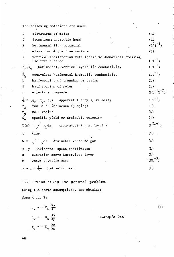
The following notations are used:

D elevations of moles

d downstream hydraulic head

F horizontal flow potential

h elevation of the free surface

i vertical infiltration rate (positive downwards) crossing

%,KV horizontal, vertical hydraulic conductivity

i$, equivalent horizontal hydraulic conductivity

L half-spacing of trenches or drains

1 half -spacing of moles

p effective pressure

the free surface

1

+ 9 = (qx, 3, 4,) r radius of influence (pumping)

r well radius

S

T ( z ) = f P h d z ' i-i'&,r SL,,; ; i i - ~ i '; 3 1 ; ~ - ' J ~ ~ ~ 7

t time

W = ,f S dz drainable water height

x, y horizontal space coordinates

apparent (Darcy's) velocity

A

P

Y specific yield or drainable porosity

z - .

h

O Y

z elevation above impervious layer

p water specific mass

@ = z i- ' hydraulic head pg

1.2 Formulating the general problem

Using the above assumptions, one obtains:

from A and B:

(Darcy ' s law)

68

from C :

y, = y,W

K = K (z) v v

s = s (2) Y Y

from D , w i th no i n t e r n a l sources and s inks :

3 + - a% + - - - O .(mass balance) ax a Y a Z

from E :

q z = o ; z = o

from F :

$ = z ; z = h

from G : t h e v e r t i c a l boundary cond i t ions w i l l be descr ibed la te r

from H:

(3)

( 4 )

(5)

Formula ( 6 ) i s a s p e c i a l mass balance equat ion on t h e f r e e su r face . A proof

of i t can be found i n Wolsack (1976) .

1 . 3 The horizontal flow potential

Charnyi (1951) was t h e f i r s t t o i n t roduce a h o r i z o n t a l flow p o t e n t i a l f o r

t h e s tudy of f i l t r a t i o n between two d i t c h e s . Guyon (1964) has used t h i s con-

c e p t s i n c e 1963 f o r drainage s t u d i e s . Here, t h e p o t e n t i a l must be def ined as

by Zaoui (1964) i n o rde r t o t ake v e r t i c a l he t e rogene i ty i n t o account:

69

D i f f e r e n t i a t i n g ( 7 ) w i t h r e s p e c t t o x o r y , one o b t a i n s :

.aF - ax

a Y aF -

Using ( 1

aF - ax

aF a Y -

and (5) :

h - _ - J qxdz,

h = - / qydz

O

Equat ion (8) shows t h a t t h e g r a d i e n t of F equa l s t h e nega t ive

v e r t i c a l i n t e g r a l of t h e apparent v e l o c i t y . F i s thus t h e hor

p o t e n t i a l of t h e cons idered problem.

D i f f e r e n t i a t i n g aga in wi th r e s p e c t t o x o r y , one o b t a i n s :

Eva lua t ing t h e i n t e g r a l :

va lue of the z o n t a l f low

Using ( 4 ) and (6) :

a2F a2F - aw i . a t ax2 a Y 2

70

1.4 The general method

The general method for obtaining drainage formulas involves the following

steps :

(i) Evaluate (exactly or approximately), using ( 7 ) , the potential F as a function of h on the vertical boundaries and on some remarkable verticals of the considered situation (chose on which the free surface is the highest, mainly).

(ii) Solve Dirichlet's problem for F,.formulated by (9) and the boundary. conditions obtained at step (i).

(iii) Compare expressions of F on the remarkable verticals, as obtained at steps (i) and (ii). One then obtains an approximate formula in which the free surface elevation is connected with the data of the situation.

1.5 The equivalent horizontal hydraulic conductivity

If the pressure distribution on each vertical were hydrostatic (Dupuit's as- sumption), one would obtain, from (7):

h F = J 5 ( z ) (h - Z ) dz

O

In addition, if the soil were homogeneous, one wouEd have:

From the above considerations, the equivalent horizontal hydraulic conductiv-

ity is defined by:

- \ ( z ) = - \ (2') dz! =.- J Z T ( z ' ) dz'

z 2 O

It follows that, where the hydrostatic pressure d,istribution can lie assumed

as a first approximation of the actual ?ressure distribution, a first appro-

ximation of F will be:

Coming back to a more general situation, a second expression of F can be de-

rived as follows:

integrating (7) by parts, with - = : :: Kh

using ( 5 ) , and because T(o) = O, one obtains:

a@ a Z

h F = T ( ~ ) ( l - -)dz

combining with (IO), (12) can also read:

From this, a third expression of F can also be derived:

again integrating by parts, and because (from (10))

d z 2 - - dz (F K (z)) = T(z):

hence:

The (exact) expressions (12) and ( 1 3) will be used in the applications to evaluate F approximately on some remarkable verticals.

72

1.6 Solv ing Dirichlet's problem

Step (ii) consists in solving the problem formulated by:

; (X,Y)@B a2F a2F aw i ax2 ay2 - + - = _ -

at

( 1 4 )

F = F1 (x,Y) ; ( X , Y ) E 9

The classical Green's method is used: introducing a "test-function" G, one obtains :

) dxdy = J9G (at aw -

Using Green's identity, one obtains:

a2G a2G F (- + -) dxdy =

Taking G equal to the Green's kernel of point (x',y'), i.e. the solution

o f :

a2G a2G

ax2 ay2 - (- + -) = 6(x - x') 6 (y - Y') ; ( x , y ) E 9

G = O ; ( X , Y ) E 9

One obtains, ,combining ( l 4 ) , ( 1 5) and ( 1 6) :

' > E B ( 1 7 ) aw aG F(x' ,Y') = j9G (i - -1 at dxdy - F1 ;i;; do(x,y) ; (x',y

For the applications (except for the pumping test), one will'use (17) with an appropriate choice of (x',~'). For the pumping test, one will use (15).

73

dxdy

2. Applications (steady-state)

2,.1 Trenches attaining the impervious layer

The.flow is invariant with any translation parallel to Oy. Space coordinates

x and z only are to be used.

-+

F i g . I . Trenches reaching the impervious layer.

One denotes (Fig.]) L the half-spacing of the trenches and d the water

level in the trenches. The free surface is the highest at x = O (elevation h ) . The boundary conditions are:

O

$ = d ; O , < z < d ; x = f L (18)

íi) One has,, from’í7), ( 1 0 ) and 4 1 8 ) :

2 F (- L) = F (L) =-- (19)

d - 2 Y, (dl

At x = 0,-one has, from (12) :

7 4

a+ .T(z) ( 1 - z) d z

' q is necessarily negative at x = O. Then, from ( I ) , . % a$ is positive. In ad- a+ aZ

Z dition, -is in general maximum on the free surface (the contrary implies

existence of a very poorly permeable layer, which would have been considered

I as impervious). It follows from (6) that, in general:

I 1 Substituting into (20) and combining with (10):

One can then write, by analogy with Guyon-Thirriot (1967):

1 with O <.%!, < 7 (last inequality only probable) O

1 (ii) Taking G = - 2 IL - X I , it comes from (1 7 ) :

L2 1 F (O) = i + - (F (L) + F (- L)) 2

(iii) Combining (19), ( 2 2 ) and ( 2 3 ) :

( 2 4 3

75

The corresponding formula f o r t h e homogeneous and a n i s o t r o p i c case i s

(Guyon & T h i r r i o t , 1967):

i i L 2 = h: K ( 1 - 2 - ) + d2K '

K

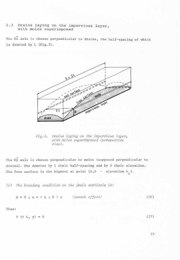
2.2 Drains laying on the impervious layer

Assuming t h e t r e n c h e f f e c t (Trench b a c k f i l l h i g h l y permeable, when compared

t o n a t u r a l s o i l ) , t h e s i t u a t i o n i s t h e same as i n Sec t ion 2 .1 ; w i th d = O

(F ig .2) .

Fig. 2. Drains Zaying on the impervious ' layer .

One d i r e c t l y o b t a i n s from (24) :

i.a0 i L2 = h2 O (ho) ( 1 - 2 ~v(ho> )

76

On the mole v e r t i c a l s the s i t ua t ion i s more complex. In the v i c i n i t y of

d ra ins , the elevat ion h (x, tl) of the f r ee surface i s smaller than D. Thus:

Far from the dra ins , h (x, t 1) i s greater than D ( a t l e a s t when the water

t ab le i s high) and tlie condition i s :

r$ = z ; y = 21 ; D < z < h (x , +L) (trench e f f e c t above mole)

Midway from the drains ( a t x = O ) , water i s flowing upwards ( a t l e a s t par-

t i a l l y ) , but t h i s flow i s cer ta in ly su f f i c i en t ly weak so tha t r$ does not ex-

ceed much D . Thus, one has, from (7) and ( I O ) : '

D2 F ( O , + I ) u - 2 'h (D)

D2 It follows tha t , on the v e r t i c a l s of moles, F i s varying from - % (DI a t

I x = O t o . 0 a t x = t L. In order t o get simple calculat ions, one assumes tha t

t h i s va r i a t ion i s sinusoidal:

2 D - F (x, t l ) E \ (D) cos (5 z) ; - L < x < + L

F ina l ly , a t ( O , O ) , one has, as a t x = O i n s i t ua t ion 2.1:

(ii) Taking G as Green's kernel of point (O,O), say:

(2p + + (2q + 1) k = P9 L2 l2

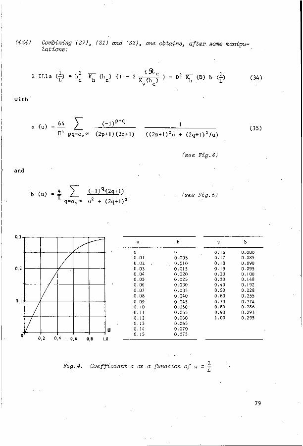
(iii) Combining (27), ( 3 1 ) and ( 3 3 ) , one obtains, a f ter , some manipu- Zations:

( 3 4 ) 2 I L l a (E) 1 = h 2 - % (hc) ( 1 - 2 - ) i s L C - D2 (D) b (E) 1 C Kv(hc)

w i t h

6 4 1 a (u) = - r14 pq=o,a (2p+1)(2q+l) (,(2p+1)2u + (2q+I)2/u>

(35)

(see F i g . 4 )

and

b (U) = - 4 (-1>q(2q+l) . . (see F i g . 5 ) n q=o,m u2 + (2q+1)2

U b U b

O O 0.01 O . 005

0.03 0.015 0.04 0.020 0.05 0.025 0.06 0.030 0.07 0.035 0.08 0.040 0.09 0.045 o . IO 0.050 0.11 O . 055 o . 12 O . 060 0.13 0.065 O . I4 0.070 0.15 0.075

0.02 , , 0.010

O. I6 O. 080 O . I 7 O . 085 O . I8 o . O90 o . 19 0.095 0.20 0.100 0.30 O . I48 0.40 0.192 0.50 0.228 0.60 0.255 0.70 0.274 0.80 0.286 0.90 O . 293 1 .o0 0.295

F i g . 4 . Coef f ic ient a as a function of u = 4 L

79

''O I- U

O 0.01 0.02 0 .03 0.04 0.05

I , 0;06 0.07 0 .08 0.09 0.10 0.11 0 .12 0.13

b -

1 O . 9998 O . 9994 0.9988 . O . 0079'

' 0.9968 O . 9954 0.994 0.992 0.990 0.988 0.985 0.982 0.979

U

OL16 0 .17 0.18 o . 19 0.20 0.30 0.40 0.50 0.60 0.70 0.80 0.90 I .o0

b

0.969 0.965 0.961 O . 957 O . 953 O . 898 0.830 0.755 0.676 0.599 O . 526 0.459 0.398

O . 14 0.976 O . 15 0.973

L F i g . 5 . Coef f ic ient b as a function of u =

~ 2.4 Well reaching the impervious layer

F i g . 6 . WeLL reaching the impervious Layer.

80

The flow is invariant by any rotation around the well axis. The horizontal

coordinate r = (x + y ) (distance to well-axis) is to be used. One de-

notes r the well-radius, d the water level in the well and h the free sur-

face elevation at r = r . One denotes rA a distance to the axis much greater than r (of the order of magnitude of the pumping radius of influence) and

h the free surface elevation in r = r There is no infiltration.

2 2 ;

P . P P

P A A’

li) The boundary condition at r = r is: P

$ = d ; O < z < d ; r = r

$ = z ; d < z < h * r = r

P

P7 P

Then, from (7) and (IO):

At r = r one has, from (12) : A’

hA a$ a Z F (TA) = o! T (z) ( 1 - - ) dz

The greater r

static distribution. One writes, by analogy with ( 2 2 ) :

the more the pressure distribution approaches the hydro- A ’

The value of 2 cannot be assessed because the pressure distribution is

very variable due to the profile heterogeneity. In addition, q, (rA, hA)

cannot be simply estimated.

One will neglect here the corrective term, and obtain then:

A

81

r Taking G = ln (F), ( 1 5 ) y i e l d s : A

(ii)

Denoting Q t h e pumping d i scha rge , one h a s , from ( 8 ) : 'I

dF Q = 2nr - A d r l r = ra ( 4 0 )

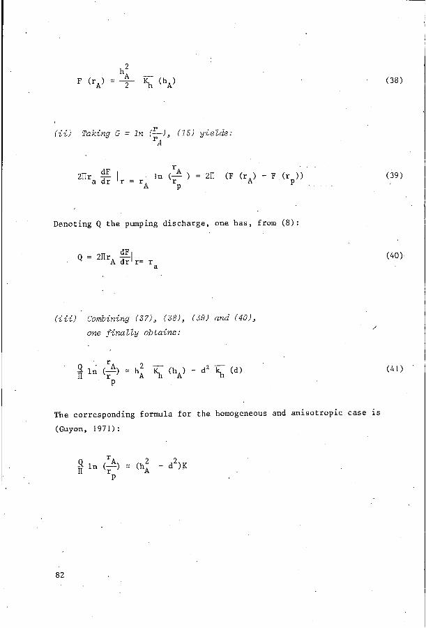
(iii) Combining ( 3 7 ) , (381 , ( 3 9 ) and (401,

one f i n a Z l y o b t a i n s : . .

(41) ' '

The cor responding .formula f o r t h e homogeneous and a n i s o t r o p i c case i s

(Guyon, 1971):

A 2

P

r 9 I n (F) 2 ( h i - d )K n

82

3 . Conclusions

Taking thexertical heterogeneity in account does not present major diffi-

culties in the applications considered here, i.e. in steady state and with

trenches, drain pipes, or well reaching the impervious layer.

In these situations, the profile heterogeneity is completely described at

first approximation with the concept of "equivalent horizontal hydraulic

conductivity". The major advantage of this concept is that the classical

formulas for.homogeneous cases can still be used, with only a slight modi-

fication: one has just to replace the homogeneous hydraulic conductivity K by. the equivalent horizontal hydraulic conductivity

However, the corrective terms of the formulas, which are generally neglected

in practice, would be more difficult to evaluate in the heterogeneous case.

in these formulas.

83

Re f e r en c e s

GUYON, G. 1964. Considérations sur l'hydraulique des nappes de drainage par canalisations enterrées. Bulletin Technique du Génie Rural 65, 45 p. + annexes.

de tarissement . C.R. Acad. Sciences Paris. 264, Série A. 43-46.

méthode de rabattement de nappe en vue des calculs du drainage. Bulletin Technique du Génie Rural 110, 29-49.

un écoulement 1 surface libre avec surface de suintement. C.R. Acad. Sciences U.R.S.S. 6.

GUYON, G., THIRRIOT C. 1967. Sur le drainage des nappes perchées en période

GUYON, G. 1971. Mesure de la conductivité hydraulique d'un sol par la

TCHARNYI, I.A. 1951. Démonstration rigoureuse de la formule de Dupuit pour

WOLSACK, J. 1976. Cours d'hydraulique souterraine. Chapt.2. E.N.G.R.E.F. Paris.

ZAOUI, J. 1964. Les écoulements en milieu poreux et l'hypothèse de Dupuit. Houille Blanche 3, 385-388.

84

Paper 1 . 0 2

SECOND AND THIRD DEGREE EQUATIONS FOR THE DETERMINATION O F THE SPACINGS BETWEEN PARALLEL DRAINAGE CHANNELS

L . F . E r n s t , I n s t i t u t e for Land and Water Management research, Wageningen, The Netherlands

S u m m a r y

The d ra inage formula proposed by Hooghoudt can be combined wi th one proposed by t h e au tho r . This r e s u l t s i n a t h i r d degree polynomial equat ion f o r t h e d r a i n spac ing . The r e s u l t i n g formula can be app l i ed t o t h e s t eady s ta te groundwater flow t o p a r a l l e l d r a i n s i n homogeneous a q u i f e r s and i n two-layer a q u i f e r s w i th t h e i n t e r f a c e a t t h e same l e v e l a s t h e open water s u r f a c e i n t h e d ra inage channels . For some th ree - l aye r a q u i f e r s t h e same equa t ion can b e used i n combination w i t h a nomograph f o r t h e r a d i a l f low r e s i s t a n c e i n a two-layer a q u i f e r . An a t tempt has been made t o o b t a i n a s impler formula by adding an empi r i ca l c o e f f i c i e n t t a t h e r a d i a l f low r e s i s t a n c e . The r e s u l t is a s l i g h t l y less a c c u r a t e second degree equat ion . A comparison of t h e s e f o r - mulae w i t h t h e r e s u l t s of Kirkham and ToksÖz d id show only s m a l l d i f f e r e n c e s . The formulae presented i n t h i s paper can t h e r e f o r e s a f e l y be used f o r p r a c t i - c a l a p p l i c a t i o n s , however wi th t h e cond i t ion t h a t t h e d r a i n spac ing must be a t l e a s t equal t o f o u r times t h e t o t a l t h i ckness of t h e . aqu i f e r .

1 . Dra inage of a h o m o g e n e o u s a q u i f e r

I n The Nether lands two formulae a r e r a t h e r widely used f o r t h e computation

of d i scha rge , d r a i n spac ing o r p h r e a t i c l e v e l . Both formulae t ake i n t o

account t h e r a d i a l flow t o t h e p a r a l l e l , h o r i z o n t a l d r a i n s .

The o l d e r formula of t h e s e two i s obta ined by assuming a completely ho r i -

z o n t a l f low, bu t i n s t e a d of t h e th i ckness H of t h e a q u i f e r between d r a i n

' l e v e l and impermeable base ( F i g . l a ) , a reduced th i ckness d ( F i g . l b ) has t o

be in t roduced t o t ake i n t o account t h e in f luence of t h e r a d i a l f low

(Hooghoudt, 1940) .

85

preclpitction ,pnreot ic surfoce,

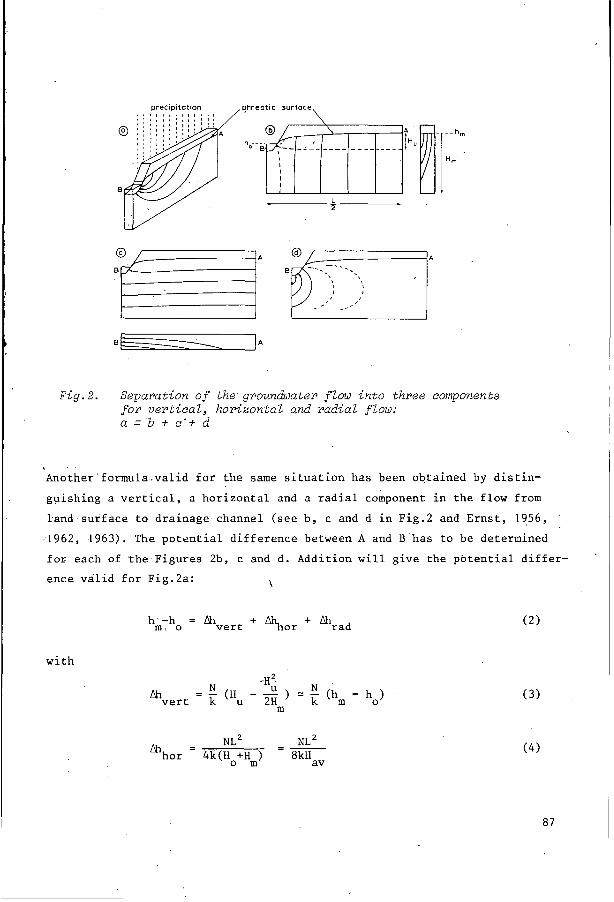
F i g . 2

- L 2 c

Separation of the. groundhater f l ow in to three components f o r ver t ica l , horizontal, and radial f l ow: a = b + c . + d

Another formula.valid for the same situation has been obtained by distin-

guishing a vertical, a horizontal and a radial component in the flow from

land surface to drainage channel (see by c and d in Fig.2 and Ernst, 1956,

1962, 1963). The potential difference between A and B has to be determined for each of the Figures Zb, c and d. Addition will give the potential differ-

ence valid for Fig.2a: \

h. m , -h o = &vert + %or + &rad

with ..H2, N U N

hvert = i; (Hu - - ) 1 - (h - h ) 2Hm k m o

NL2 = - N L ~

&hor - 4k(Ho+Hm) 8kHav

( 3 )

( 4 )

87 I

Ahad = NLR (5 )

where

Ho = thickness of the aquifer between drain leve1,and'impermeable base

Hav = average thickness of aquifer

R = radial flow resistance

~- By substitution of Eqs. 3, 4 and 5 into Eq. 2:

NL2 + NLR h - h = - ( h - h ) + - N m o k m o 8kHav ,

or

NL2 + NLR k-N - (hm-h ) = - k o 8kHav

Eq. 6 seems to be quite close to a linear relation between h -h and N,

because in nearly all practical cases the coefficient (k-N)/k will lie

between 0.9 and 1 . However, this i s not a reason to consider Eq.6 very

different from the second degree Eq.1. It should be born in mind, that

not only H is depending on h -h i.e. Hav = Ho + $(hm-ho), but that there is also a slight decrease in the radial flow resistance R for in- creasing discharge.

m o

av m o'

For the moment all non-linear effects will be discarded by assuming that

only situations with small N/k and consequently small h -h

dealt with. This implies that Eq.6 can be replaced by:

have to be m o

h - h = - NL2 + "no m o 8kHo

I 88

( 7 )

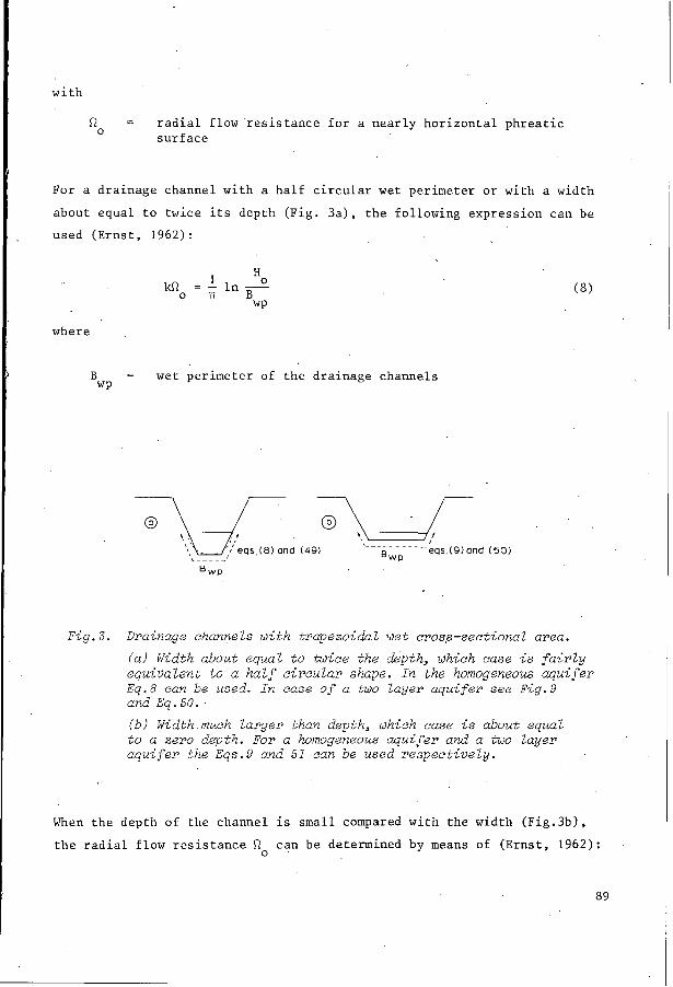
with

Ro = radial flow’resistance for a nearly horizontal phreatic surf ace

For a drainage channel with a half circular wet perimeter or with a width

about equal to twice its depth (Fig. 3a), the following expression can be

used (Ernst, 1962) :

where

B = wet perimeter of the drainage channels WP

F i g . 3. Drainage channels with trapezoidal wet cross-sectional area.

(al Width about equal to twice the depth, which ease i s f a i r l y equivalent t o a half circular shape. In the homogeneous aquifer Eq.8 can be used. In case of a two layer aquifer see Fig.9 and Eq .50.

f b l Width much larger than depth, which case i s about equal to a zero depth. For a homogeneous aquifer and a two Zayer aquifer the Eqs.9 and 51 can be used respectively.

When the depth of the channel is small compared with the width (Fig.3b),

the radial flow resistance Ro can be determined by means of (Ernst, 1962):

89

1 4Ho kS2 = - I n - o í‘r ?rB WP

0.3

0.2

O.’

O

( 9 ) ’

- 3.’; -

- ./:

The decrease of R , with an increasing discharge q = NL through each of the drainage channels, is a rather complicated problem, which has not been in-

vestigated thoroughly up to now. For a homogeneous aquifer both the depth

H of the impermeable base, the shape of the drainage channel (e.g.: slope

a, see Fig.4) and the discharge intensity q should be taken into account.

O

O

k R o - k R s q 0 1 5 & k B w p

F i g . 4 . Nomograph f o r the decrease in radial flow resistance R with in- creasing discharge q fo r a wet cross-sectional area as show in the r ight hand si2e of t h i s f igure (Ernst, 1962, . F i g . 2 8 c ) . The water depth, i s assumed t o remain constant.

The magnitude of the decrease of R can,be read from Fig.4. Because h.most

practical cases q /kB < 1, it can be assumed that this increase.is not

very important except for flat slopes and very large discharge intebsities. O w p

Another question which has still to be discussed is the applicability of

the preceding formulae on very thick aquifers. Both expressions 8 and 9

are not to be used in case of very large H /L-values. It can be seen immed- iately that use of these equations for Ho = mwould lead to h -h

is obvious, that .for increasing H

hydraulic head difference h -h

O = m. It m o

there must be a gradually decreasing with the following minimum values for the m o’

90

cases corresponding to Eqs.8 and 9 (Ernst, 1956, 1962):

NL L h - h +-ln- WP

m o ?rk B

U

Substitution of Eqs.8 or 9 in 7 and comparison with Eq.10 or 1 1 shows that

the accuracy of these equations is satisfactory if H < L/4. Formulae con-

taining radial flow resistances can therefore be accepted especially for

those practical problems in which tI /L and (h -h ) / L have no excessive va-

lues. O o m

2 . A t h i r d d e g r e e e q u a t i o n € o r t h e d r a i n s p a c i n g

Still using

can be simp

From 7 and

the assumption that N/k and h -h are relatively small, E q . 1 m o if ied to:

N L ~ h -ho = - m 8kd

2 it fo l lows immediately that

d L Ho L + 8kHoQ0 - =

T h i s expression f o r d can also be used in Eq.1 without neglecting the sec-

ond degree term. Then only one condition has to be obeyed: Ho < L/4. For

larger values of H Eq. 13 can still be used by introducing a fictitious

value H,, being about oneafourth of the presumable value of L.

Substitution of Eq. 13 into 1 gives:

\

L NL2 = 8kHo + skH (hm-ho> + 4k(hm-hj)’

O 0

91

or:

(h.-h ) hm-h 2 + (- O)

- = NL m o 16kH: ( L + 8kHoRo)2Ho

2H0

Eq.14 contains 7 varcables: N, L, k, Ho, R o y hm and ho.,By re-arranging this formula as in Eq.15 it can be seen immediately that the present rela-

tion can be considered as containing only 4 dimensionless parameter combi-

nations:

and M o N , L hm-ho - - _ _ HO

k’ Ho*’

This number can be reduced to 3 , by substituting of the following parameters

A, B I and y. Each of these parameter combinations contains only one of the

most important properties of the system: drain spacing L j. A, hydraulic head difference h -h + B I , precipitation rate N + y. m o

= A 8kHoRo

= B1 hm-ho

2H0

2Mo e = y

Substitution of Eqs. 16, 17 and 18 in 15.results in:

(19)

Eq.19 is a third degree equation in A, like Eqs.

equations in L. A rather convenient method for a

of the nomograph shown in Fig.5.

, 4 and 15 are third degree

solution of X.is making use

92

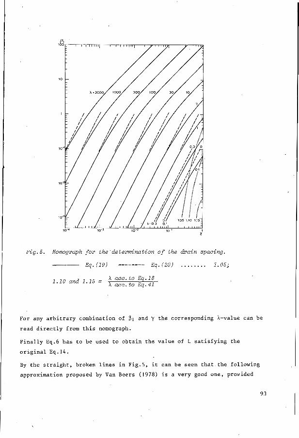
F i g . 5 . Nomograph for the 'de teminat ion of the drain spacing.

E s . ( 1 9 ) -------- Eq. ( 2 0 ) ...... .. 1.05;

X acc.to Eq .18 ' . l o and = X acc.to E q . 4 1

For any arbitrary combination of 81 and y the corresponding A-value can be read directly from this nomograph.

Finally Eq.6 has to be used to obtain the value of L satisfying the orcginal Eq. 14.

By the straight, broken lines in Fig.5, it can be seen that the following

approximation proposed by Van Beers (1978) i s a very good one, provided I

93 I

B I < 0.1 and X > I ' .

or

In view of the fact that there is a large 'range of conditions for which the

accuracy of Eqs.20 and 21 is not satisfactory, these equations will not be

considered furthermore in this paper.

The increasing elevation of the phreatic surface with increasing precipita-

tion must result in a non-linear relation between N or U and h -h . This has been taken into account by -Hooghoudt (Eq.1) by assuming that the

flow in the ground above drain level is the main reason for the non-linear

behaviour. Neglect of the vertical component of the flow above drain level

is not always allowed. The vertical flow is of importance if 0.2 < N/k < 1

and also in two-layer aquifers with a rather small hydraulic conductivity in the upper region. Whatever the importance may be, the vertical flow com-

ponent can be taken properly into account by addition of a coefficient

k/(k-N), as has been shown by Eqs. 3 and 6 (Ernst., 1 9 5 6 ; Kirkham, 1 9 6 1 ) .

m o

It is obvious that this coefficient should also be added to Eqs. 1 and 14

respectively resulting in:

and

h ) 2 + 8d(k-N)(h

L2

- L2 = L + L 8kHoRo . 8Ho (hm-ho) + 4 (hm-ho) ' k-N

Eq.19 remains valid. Only the expression for the parameter y has to be

changed a little:

9 4

y = 2kR O

In the analysis achieved by Kirkham and ToksÖz (Kirkham, 1958; ToksÖz and

Kirkham, 1971a and 1971b) the horizontal flow above drain level has been ne-

glected, which implies that d2h/dN2 > O. This involves that a comparison of these results with Eq. 23 should be done in the first place for N << K.

Under this condition Kirkham's formula (Kirkham, 1958) and Eq.23 will give

practically equal results except for H Eq.7 with 8 or 9 is failing.

> L/4, where the combination of

3 . The inflection point in the h (N)-relation m

In many practical cases a linear relation between N=U and h -h can be assu- m o med without the implication of large errors. Introduction of special assump-

tions for the flow direction above drain level - horizontal flow or vertical flow - will result in non-linear relations with exclusively negative or ex- clusively positive values for the second derivative d2h/dN2.

In the preceding chapter it has been shown, that from a fundamental point of view a more satisfactory relation can be obtained by means of the third de-

gree Eq.23, with both positive and negative values of the second derivative

d2h/dN2. The conditions under which for practical application a linear or

non-linear relation might be assumed, can be most easily discussed by writing

equation 22 in a slightly different way:

4 [( hm - ,". + d)2 - fi)j= N k-N

Equation 25. can also be written as:

(25)

95

. h,-h,+d L

O2 0.4 0.6 0.8 1.0 N k -

F i g . 6.. ReZation between hydrauZic head h -h and precipi tat ion m o surplus N dependent on d, L and k according to Eq.25.

- - - _ _ - locus of infZection points.

I n each i n f l e c t i o n p o i n t t h e second d e r i v a t i v e must ,be . equal t o zero :

By e l i m i n a t i o n of a , from Eqs. '26 and 27 , t h e locus of t h e i n f l e c t i o n p o i n t s

i s found t o be:

h,-ho + d

L 4

Eq.25 and t h e locus of i n f l e c t i o n p o i n t s accord ing t o Eq.28 are shown i n

F ig .6 . It can be seen t h a t a marked cu rva tu re is only p o s s i b l e f o r r e l a t i v -

e l y l a r g e v a l u e s of (h -h ) / L o r (and) d/L. According t o Hooghoudt's t a b l e s m o

96

I n Chapter 1 t he v e r t i c a l component of t he flow above the d r a i n l e v e l has

been taken i n t o account by Eq. 3. The p o t e n t i a l d i f f e r e n c e f o r t he v e r t i c a l

f low i n t h e upper l a y e r can now be expressed by:

r 1

Analogous t o the c a i e of t h e homogeneous a q u i f e r a s i m p l i f i c a t i o n of t h e 1

expression f o r BI can be accepted by neg lec t ing t h e second term between . v e r t

t h e b racke t s , giving:

N & v e r t . - kl (hm-ho)

- -

The v e r t i c a l flow can be incorporated i n t h e Hooghoudt formula by adding

& v e r t Sion s i m i l a r t o Eq.22:

t o t h e p o t e n t i a l d i f f e r e n c e used i n Eq.29. The r e s u l t i s an expres-

k N - U - 8 -2 k i d(hm-ho) + 4(hm-ho)2 -

L2 kl-N kl-N

The expression which has t o be s u b s t i t u t e d f o r d can be.found again i n

13, bu t now with proper s u b s c r i p t s :

S u b s t i t u t i o n of Eq. 33 i n 32 and re-arranging r e s u l t s i n :

2k2H2L - I = (34) N L ~

ki (hm-ho> (L+8k2H2Qo) 4(ki-N) (hm-hol2

P r i n c i p a l l y t h e r e i s no d i f f e r e n c e between E q s . 1 4 and 34. Therefore Eq.19

and F ig .5 can be used again f o r a s o l u t i o n of L. For A , BI and y t h e

fol lowing expres s ions , s l i g h t l y d i f f e r e n t from those used be fo re , hold:

98

5. Simplified expression for the drain spacing

Some at tempts have been made t o o b t a i n simple expressions f o r t h e d r a i n

spacing. The f i r s t at tempt w a s made by adding an empir ical c o e f f i c i e n t t o

t h e l a s t t e r m of equat ion 7 :

+ B2NLRo NL

hm-ho - 8k2H2 + 4kl(hm-ho)

w i t h

The i n t r o d u c t i o n of t h e c o e f f i c i e n t 8 2 w a s done with t h e i n t e n t i o n t o avoid

t h e use of more complicated e x p r e s s i o n s , f o r R. This r e s u l t s i n an equat ion

of t h e second degree i n L :

However, Eq. 40 i s only s u f f i c i e n t l y accu ra t e i f y 2 2klLo < O . 1 . This

i s enough reason t o r e j e c t Eq.40.

By so lv ing L L from Eq. 7 , adding a second degree term i n h s imilar t o Eq.1

and using t h e r a d i a l flow r e s i s t a n c e B2Q0 s imi la r t o Eq.38, a s impl i f i ed

expres s ion of s a t i s f a c t o r y accuracy has been obtained, namely:

NL2 = 4 k 1 ( h , - h ~ ) ~ + N

99

. .

Introduction of similar parameters A, 61 and y as before, however with J N T

instead of JN/(k -N), permits a shorter writing of the last formula: 1

,

2 klQo& 1 = y

Eqs. 41 and 4 2 may give some advantage when a calculation of A is required and no nomograph is available. The rather smal? diffcrcnccs In y-values according to Eqs.19 and 4 2 are shown by the dotted lines in Fig.5. -Errors

of more than 5% will only occur when A < 1 and y > 0.3.

6. The drain spacing €or a three-layer aquifer

Because Eq. 34 is applicable to two-layer aquifers, with the restriction

that the interface between the two layers has to be of the same depth as the level of the open water, it seems profitable for practical application to

also investigate the case of an interface below the bottom of the drainage

channels.

This can be done by immediately passing over to the consideration of

three-layer aquifers as shown in Fig.8.

I O0

1 o2

Fig.9 is showing a nomograph by means of which a determination of radial

flow resistance in two-layer aquifers can be obtained. In this nomograph

only k Ik or shape of the drainage channel and the phreatic surface are neglected

(ERNST, 1962, 1963).

and H3/H20 are considered as variables, while variations in size 3 2

.Fig. 9 depends mainly on two assumptions:

1 . use of a special value BI = H20 and

2. small values for the discharge.q s o that variations, comparable Wp

to what has been shown in Fig.4,'are of no importance. .

Only for these conditions Fig.9 is giving immediately the corresponding

radial flow resistance R' For arbitrary values of the wet perimeter B but anyhow not larger than H

20' computed by means of Eqs.50 or 51:

20 ' , , Wp' the real radial flow resistance R20 can+be

in which formulae:

R 2 0 = radial flow resistance for a two layer aquifer with a

Hz 0 = thickness of layer with permeability :k2 between- drain level nearly horizontal phreatic surface

and lower boundary of this layer

Which of the last two Eqs. has to be applied -depends on the general shape of the channel, respectively for relatively deep and.relatively shallow

channels as shown in Fig.3.

7 . Discussion

Use of equations with logarithms - like Eq.8 or 9 - for the determination of the radial flow resistance R may cause relatively large errors. Thls

O

might be considered as a major imperfection in the presented system. In

order to show to which extent this is an objection for practical use, E q s .

7 and 8 will be applied on the drainage .situation in a homogeneous aquifer

(Fig. I O ) .

. , , / ,

0 according io eqs. ?and 8 - L +I,, K .

, , 8 H lT L . .

/ . 0.1 0.2 0.3 0.4 0.5 0.6 0.7 0.8 0.9 1.0

u

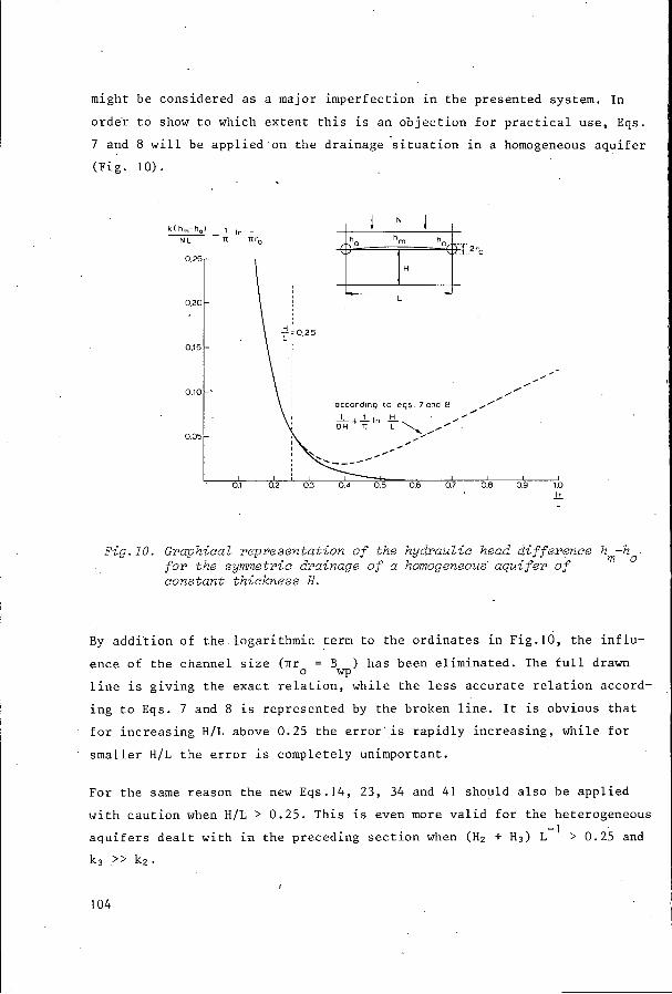
Fig.10. Graphical r epresen ta t ion of t he hydraul ic head d i f f e r e n c e hm-ho for t he symmetric drainage of a homogeneous’ aqu i f e r of constant t h i ckness H .

By addition of the logarithmic term to the ordinates in Fig.10, the influ-

ence of the channel size (nro = B ) has been eliminated. The full drawn

line is giving the exact relation, while the less accurate relation accord-

ing to E q s . 7 and 8 is represented by the broken line. It is obvious that

for increasing H/L above 0 . 2 5 the error’is rapidly increasing, while for

smaller H/L the error is completely unimportant.

Wp

For the same reason the new E q s . 1 4 , 2 3 , 34 and 41 should also be applied

with caution when H/L > 0 . 2 5 . This is even more valid for the heterogeneous

aquifers dealt with in the preceding section when (H2 + H3) L-’ > 0 .25 and

k3 >> k 2 .

104

Some au thor s (HOOGHOUDT, 1940; VAN BEERS, 1965) have s t a t e d t h a t i t makes

h a r d l y any d i f f e r e n c e i f t h e a q u i f e r a t a depth below 0.25 L i s permeable

o r impermeable. Neglect ing t h e deeper p a r t of t h e a q u i f e r i s f a i r l y c o r r e c t ,

i n a l l t hose cases i n which t h e a q u i f e r below 0.25 L w i l l not have a very

l a r g e conduc t iv i ty .

' has no t t o b e confused with t h e . a p p l i c a b i l i t y of t h e drainage formulae pre-

1 sen ted i n t h i s paper. The s ta tement t h a t t hese formulae should not be used I

f o r very t h i c k a q u i f e r s (H/L > 0.25) has t o be maintained. This r e s t r i c t i o n

can ha rd ly be weakened f o r r e l a t i v e l y s m a l l d r a i n s , because even f o r

B

u s e of t h e s e formulae w i l l r e s u l t i n a 25%-error.

/L = 0.003 wi th HI/L=I, H /L=l and k /k = I O , i t can be shown t h a t a p l a i n 2 2 1

I n o r d e r t o show t h e in f luence of t he permeabi l i ty of deeper l a y e r s , e.g.

below a depth 0,.25 L, Fig.11 has been constructed by means of a v a i l a b l e

exac t information (KIRKHAM, 1961; TOKSUZ and KIRKHAM, 1971 b ) . This f i g u r e

g i v e s a comparison of r equ i r ed hydrau l i c head d i f f e r e n c e s f o r two-layer

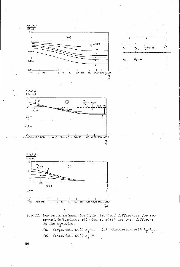
a q u i f e r s , which are only d i f f e r e n t i n k2-values. The small H /r -values

given i n t h i s f i g u r e , do not occur under p r a c t i c a l cond i t ions . When H /r =

8, i t fol lows t h a t B / L = O . I .

1 0

I o

WP '

By F i g . l l a i t i s shown t h a t t he assumption of impermeabili ty below a depth

L/4 can be r a t h e r bad, e s p e c i a l l y f o r small H f r -values which are not l i k e l y I o ' t o e x i s t . Even l a r g e r e r r o r s have t o be expected when t h e second l a y e r i s

neglected f o r va lues of HI/L smaller than 0.25.

From F i g . l l b it can be concluded, t h a t i n case of a complete ignorance about

t h e deeper l a y e r s , t h e e r r o r s w i l l s t a y between f a i r l i m i t s by assuming t h a t

t he ' pe rmeab i l i t y k a l s o holds f o r t h e deeper l a y e r s below L/4.

F i g . l l c shows t h a t i n t roduc t ion of k2 = 00 can only be recommended i n those

c a s e s t h a t k2 /k l > 3 .

A main r e s u l t of Fig.11 i s t h a t i t shows t h e r e l a t i v e l y l a r g e in f luence of

t h e H / r -values on t h e magnitude of t h e e r r o r s caused by in t roduc t ion of

wrong va lues f o r k2. When r e l a t i v e l y l a r g e d r a i n s a r e excluded, some igno-

rance about t h e deeper l a y e r s i s much less harmful.

F i n a l l y i t must be born i n mind t h a t t h e ques t ion about t h e e r r o r s caused

by inaccura t e va lues f o r t h e hydrau l i c conduc t iv i ty of t h e deeper l a y e r s ,

1

1 0

o

I 2 0.9 -

, ,

YO.8 -

0.7 , . I I I I I 1 1 . 1 "... 0.1 *.-.0.2.0.5. ..l.. -.... 2 .5.,:r.,10..-:.20 50 . ,100 ..200.500~1000

- k 2 k t

I I

I I

I I

h ( k , , k 2 J

h( kl F" 12

1024

09-

oe. 1 1 1 1 1 1 1 1 1 1 1 O1 O 2 0 5 1 2 5 210 20 5 0 100 200 500 1000

- k2 k,

F i g . 1 1 . The r a t i o between the hydraulic head differences f o r two symmetric drainage s i tuat ions, which are only d i f ferent i n the k2-value. -(a) Comparison with kZ=O. ( b ) Comparison with k,=k,. (e) Comparison w i t h ka=..

106

References

VAN BEERS, W.F.J. 1965. Some nomographs for the calculation of drain spacings. Bull. 8, Int. Inst. for Land Reclamation and Improvement, Wagenin- gen. pp.48.

Inst. for Land Reclamation and Improvement, Wageningen (in press).

cross sections. Neth. J.Agr. Scí. 4: 126-131.

ning bij aanwezigheid van horizontale evenwijdige open leidingen (Groundwater flow in the saturated zone and its calculation when parallel horizontal open conduits are present, with English summary). Thesis, University Utrecht, pp. 189.

open leidingen (The calculation of groundwater flow between paral- lel open conduits, with English summary). Committee for Hydrolo- gical Research TNO, The Hague, Proceedings and Informations 8: 48-68.

BEERS. W.F.J. 1979. Computing drain spacings, Bull. 15 (revised edition), Int.

ERNST, L.F. 1956 Calculation of the steady flow of groundwater in vertical

ERNST, L.F. 1962. Grondwaterstromingen in de verzadigde zone en hun bereke-

ERNST, L.F. 1963. De berekening van grondwaterstromingen tussen evenwijdige

HOOGHOUDT, S.B. 1940. Bijdragen tot de kennis van enige natuurkundige groot- heden van de grond, deel 7 (Contributions to the knowledge of some physical properties of the soil, part 7) Versl. Landb. Onderz., Ministry of Agriculture, The Hague 46(14): 515-707.

KIRKHAM, D. 1958. Seepage of steady rainfall through soil into drains.

KIRKHAM, D. 1961. An upper limit for the height of the water table in drain- Trans. Amer. Geohpys. Un. 39: 892-908.

age design formulas.,Trans. 7th Int. Congr. Soil Sci., Madison 1960, Vol. 1 : 486-492.

LABYE, Y. 1960. Note sur la formule de Hooghoudt. Bull. Techn. du Génie

TOKSUZ, S. and D. KIRKHAM. 1971a. Steady drainage of layered soils: part I,

TOKSUZ, S. and D. KIRKHAM. 1971b. Steady drainage of layered soils: part 11,

Rural, Min. de l'hgriculture de la R6p. Française, 49.1, pp. 21.

Theory.' Journ. Irrig. Drain. Div., ASCE. Vol. 97, nr. IRI:I-18.

Nomographs. Journ. Irrig. Drain. Div., ASCE. Vo1.97, IRI: 19-37.

Paper 1.03

DRAINAGE CALCULATIONS IN STRATIFIED SOILS USING THE ANISOTROPIC SOIL MODEL TO SIMULATE HYDRAULIC CONDUCTIVITY CONDITIONS

J. H. Boumans , EUROCONSULT, Arnhem, The Nether Zands

Summary

Drainage often occurs in alluvial plains, which are characterized by layered soils that have different hydraulic conductivities for horizontal and for vertical flow.

The generalIy applied calculation models, assuming isotropic, permeable soils are not suitable to simulate the drainage flow in layered soils. Drainage in such soils can be more suitably calculated by means of anisotro- pic soil models. Moreover, the anisotropy approach offers the advantage that the otherwise difficult and often arbitrary choice of the depth of the im- permeable layer is of less significance. Accounting for soil anisotropy in drainage calculations is relatively easy as anisotropic models can be reduced to know isotropic calculation models,by simple transformation rules.

in drainage calculations, the determination o f the horizontal and vertical hydraulic conductivity components, data on soil anisotropy from literature and collected in the field.

The article further discusses the theory and application of anisotropy

1. Introduction

Drainage problems usually occur in alluvial plains. Alluvial soils are

characterized by macro and micro stratification. Drainage calculations are mostly based on one or two layer models assuming isotropic soil conditions.

These models are not very suitable to simulate the drainage flow in strati-

fied soil layers. They neglect anisotropy resulting from micro stratifica-

tion and can only consider the effect of macro stratification on the drainage

flow to a very slight extent.

\

108

It is believed that the anisotropic soil model is better suited to

approach the actual conditions in a stratified soil and is, therefore, to

be preferred for this exercise.

The introduction of soil anisotropy in drainage calculations for strat-

ified soils is no new feature. Israelsen and Hansen (1960) have drawn atten- tion to the anisotropy of alluvial soils. Lindenbergh (1963), and Boumans

(1963) have also reported on this feature. Application of anisotropy in

drainage, has, however, found little application so far. This paper discus-

ses different aspects of the anisotropy model.

2 . D e f i n i t i o n s and t h e o r y of s o i l a n i s o t r o p y

)

2 . 1 D e f i n i t i o n s and basic p r i n c i p l e s

If the hydraulic conductivity (K) in a soil is not,the same in.all

directions, such soil is anisotropic. For practical reasons anisotropy i s

limited to a different K for the horizontal flow (Kh) and f o r the vertical

flow (Kv).

The theory of the flow through anositropic media has been studied by

several authors. The available knowledge was reviewed by Maasland (1957)

who also discusses applications and implications for the groundwater drain-

age.

Application of anisotropy in drainage calculations is in fact simple,

as any homogeneous anisotropic soil medium can be transformed into a ficti-

tious isotropic medium by easy rules. Transformation makes it possible t o

apply the available drainage formulas which take into account two dimensio-

nal flow for isotropic soil as well as for anisotropic soil. For formulas

based on one dimensional horizontal flow only, e.g. the Donnan equation

( 1 9 6 4 ) , transformation has no sense and does not affect results.

1 o9

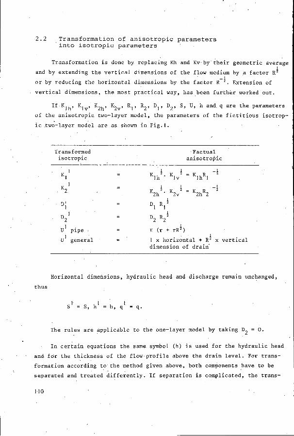
2.2 Transformation of anisotropic parameters into isotropic parameters

Transformation is done by replacing Kh and Kv by their geometric average I

and by extending the vertical dimensions of the flow medium by a factor R'

or by reducing the horizontal dimensions by the factor R-'. Extension of

vertical dimensions, the most practical way, has been further worked out.

If Klh, Klv, K2h, K2v, RI, R 2 , DI, D 2 , S, U, h and q are the parameters of the anisotropic two-layer model, the parameters of the fictitious isotrop-

ic two-layer model are as shown in Fig.1.

Transformed Factual is0 tropic anisotropic

1

1 K2

I ' D2

I I I -_ Klhz. KIV4 = K Ih R 1

I - - I - I K2h'. K2v' = KZhR2 *

I - - Dl R,'

I - - D2 R 2 %

Horizontal dimensions,

thus

I - - 71 (r + rR') 1

1 U pipe

U general I - - 1 x horizontal + R' x vertical

dimension of drain'

1 SI = S, h = h, q

hydraulic head and discharge remain unchanged,

= q .

The rules are applicable to the one-layer model by taking D2 = O. I

I n certain equations the same symbol (h) is used for the hydraulic head

and for the thickness of the flow profile above the drain level. For trans-

formation according to the method given above, both components have to be

separated and treated differently. If separation is complicated, the trans-

1.1 o

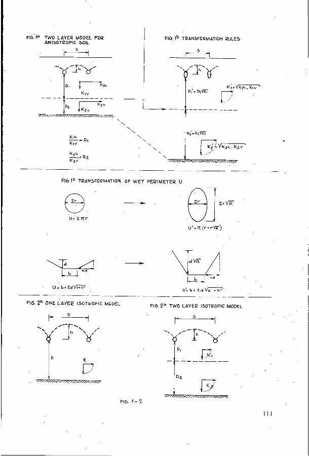
FIG.-IQ TWO LAYER MODEL FOR ANISOTROPIC SOIL

FI6. f b TRANSFORMATION RULES i i - 5 I

1 I 7’

- - ____ _____ ~ ____

61Gic TRANSFOPMATION OF WET PERIMETER U

KJd - vw/ I* I b,T-

U=. b c 2 d m U; b c Z d G x 7 ’

FIG. 2” ONE LAYEP ISGTkOPiC MGDEL F I G 2b TWO LAYEP ISOTROPlC MODEL

5 F I

1 1 1

formation method, in which the horizontal dimension are reduced and the

vertical ones remain unchanged, is to be preferred.

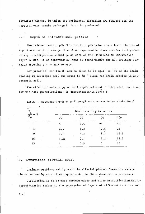
2 . 3 Depth of relevant s o i l profile

- The relevant soil depth (RD) i s the depth below drain level that is of

importance to the drainage flow if no impermeable layer occurs. Soil permea-

bility investigations should go as deep as the RD unless an impermeable

layer is met. I f no impermeable layer is found within the RD, drainage for- mulas assuming D = 00 may be used.

For practical use the RD can be taken to be equal to 114 of the drain - I

spacing in isotropic soil and equal to i R

sotropic soil. times the drain spacing in ani-

The effect of anisotropy on soil depth relevant for drainage, and thus

for the soil investigations, is demonstrated in Table 1 .

TABLE I . Relevant depth of soil profile in metres below drain level

~~~~ ~~~

Drain spacing in metres - R Kh

KV 20 50 1 O0 zoo - -

1 5 12.5 25 50

4 2.5 6.2 12.5 25

9 1.7 4.2 8.3 16.6

16

25

1.25 3.1 6.2 - 12.5

1 2.5 5 10

3 . Stratified alluvial so i l s

, Drainage problems mainly occur in alluvial plains. These plains are

characterized by stratified deposits due to the sedimentation processes.

Distinction is to be made between macro and micro stratification.Macro-

stratification refers to the succession of layers of different textures and

112

physical properties in the profile, micro stratification to the platy or

laminated structure of the separate layers. Both macro and micro stratifica-

tion can be observed in soil pits and borings.

Alluvial soils are not only heterogeneous in vertical direction, they

also show a great variation horizontally. Soil profiles vary from place to

place. Soil strata are seldom found continuously over a large area. They

often occur in lenses of a limited extent or are intersected by other depos-

its. . .

4. The drainage model for i so t ropic soil

The actual flow of groundwater to drains in the fields is very complic-

ated. For practical application, s o i l and flow conditions have to be reduced

to simplified simulation models. The models commonly used for drainage de-

sign purposes are:

the one-layer isotropic soil model of Fig.2, for which solutions are available for steady state and non-steady state flow assumptions, such as the Hooghoudt and Ernst formulas for steady state and the modified' Glover-Dumm and Krayenhoff van de Leur-Maasland formulas for non-_steady state conditions;

the two-layer isotropic so i l model of Fig.la for which steady state solutions by.Ernst and ToksÖz-Kirkham are available.

The isotropic models are not suited to simulate flow conditionS.in

stratified alluvial soils for the following reasons:

only two permeable layers can be accounted for although often more

- the depth of the impermeable layer, an essential parameter in this model, is difficult to assess. Impermeability in the sense of the model is a complex notion depending on the relative permeability of a layer but also on its thickness and depth in the profile and on the extension and variation of these characteristics in horizon- tal direction.

soil anisotropy due to micro stratification is neglected;

than two occur in the soil depths relevant for drainage;

1 "modified" re f e r s t o the repZacement of depth D by the equivaZent depth d of Hooghoudt t o account f o r radia2 f l o w

113

5. The drainage model for anisotropic soil

I n t h e a n i s o t r o p i c one- and two-layer drainage model, t h e l a y e r s are

assumed t o be homogeneous. These models are b e t t e r s u i t e d t o s imula t e t h e

hydrau l i c conduc t iv i ty cond i t ions i n s t r a t i f i e d s o i l .

Anisotropy due t o m i c r o - s t r a t i f i c a t i o n can be taken i n t o account, t h e

e f f e c t of t h e complex m a c r o - s t r a t i f i c a t i o n can be simulated a s - a p p a r e n t ani-

so t ropy , and t h e depth of t h e impermeable l a y e r i s less c r i t i c a l .

The d i f f e r e n t components of t h e K i n t h e an i so t ropy model of a s t r a t i -

f i e d s o i l ( s e e Fig.3) are:

t h e Kh and Kv of t h e separate-homogeneous a n i s o t r o p i c s o i l l a y e r s : Knh and Knv;

t h e average Kh and Kv of t h e s t r a t i f i e d p r o f i l e .

- .sum Dn Kv = sum Dn Dn

sum (Knh . Dn) Eh = sum - Knv

t h e weighed average kh o r kv of a s e c t i o n o r a r e a f t a k i n g i n t o account t h e v a r i a b i l i t y i n h o r i z o n t a l d i r e c t i o n ;

t h e average depth of t h e impermeable l a y e r i f . s u c h l a y e r .occurs w i t h i n t h e r e l evan t s o i l depth.

6. Determination of the hydraulic conductivity components

-6.1 Undisturbed samples

Kh and Kv of t h e s e p a r a t e s o i l l a y e r s can be measured i n undis turbed

s o i l samples. Average Kh and Kv va lues of t h e p r o f i l e and of areas are

f u r t h e r , f o u n d by c a l c u l a t i o n . Applicat ion of t h e method i s l i m i t e d by the

d i f f i c u l t y of ob ta in ing a l a r g e number of undis turbed s u b s o i l samples and

by t h e l a r g e random e r r o r of t h e measurements due t o t h e small sampling

volume.

114

H.C. RELATIONSHIPS

4,.2,3 ---: = n =NUMBER OF SOIL L4YER

1,n .m -----=m= NUMBER OF SOIL BORING (PR0FILE.S)

DE =THICKNE55 OF 501LLAYER h I N PROFILE

K h h =HOEIZONTAL H.C. 501L LAYER n

Knv= VERTICAL H.C. SOIL LAYER n

AVEPAGE HORIZONTAL AND VERTICAL H C OF SOIL PROFILE AT BORING I

Z K h n 0: - K h I = +z D:

2 D Z D hr

Kun

- KvI =

c-

AVERAGE HORIZONTAL AND VERTICAL H.C. OF A SECTION OR AREA

\ Kv = ,,,

I \

115

6.2 ' Pumping tests

Pumping t e s t s can p rov ide d a t a on t h e average Kh and Kv of a r e l a t i v e l y

l a r g e s o i l volume.

I f t h e w e l l f u l l y p e n e t r a t e s i n t o t h e a q u i f e r , t he t e s t p rov ides t h e Kh provided t h a t t h e depth of t h e a q u i f e r i s known.

I f t h e w e l l p a r t i a l l y p e n e t r a t e s i n t o a non-confined a q u i f e r , t h e t e s t may provide d a t a on t h e average h o r i z o n t a l and v e r t i c a l H.C. components.

v e r t i c a l h y d r a u l i c c o n d u c t i v i t y of t h e semi-permeable upper s t r a t a provided t h a t t h e t o t a l depth of t h e s e s t r a t a i s known.

A w e l l t es t i n a semi-confined a q u i f e r s u p p l i e s d a t a on t h e average

6.3 The augerhole method

The augerhole method accord ing t o E r n s t and Kirkham can be used i n f i e l d

measurements of t h e average h o r i z o n t a l pe rmeab i l i t y of t h e s o i l below t h e

groundwater t a b l e . A s t h e methods have been developed f o r homogeneous i so -

t r o p i c s o i l c o n d i t i o n s , t h e a c t u a l Kh

K , Kh = CK.,The c o r r e c t i o n f a c t o r C 'ha

p r a c t i c a l a p p l i c a t i o n i t can mostly be neg lec t ed as i t s e f f e c t on t h e d r a i n

spac ing , be ing p r o p o r t i o n a l to t h e f o u r t h r o o t of C y i s v e r y s l i g h t .

s i n f a c t h ighe r t han t h e measured

been ana lysed by Maasland ( 1 9 5 7 ) . For

6.4 Piezometer data

Hydraul ic head d i f f e r e n c e s observed i n p iezometers placed on top o f , and

below permeab-le s o i l s t ra ta supply informat ion on t h e Kv of s e p a r a t e , o r com-

b i n a t i o n s of , s o i l l a y e r s . I f t h e cor responding upward o r downward ground-

water f low rate i s known, Kv can be c a l c u l a t e d .

6.5 Indirect methods

I n d i r e c t methods such a s e v a l u a t i o n of h o r i z o n t a l and, v e r t i c a l permea-

b i l i t y on t h e b a s i s of t e x t u r e o r by v i s u a l a p p r a i s a l of s o i l s t r u c t u r e and

m i c r o - s t r a t i f i c a t i o n a r e ve ry u s e f u l , e s p e c i a l l y i f they s e r v e t o i n t e r p o l a t e

o r e x t r a p o l a t e o t h e r d a t a .

116

6.6 Measurements on existing drains

Analyses of t h e d i scha rge - h y d r a u l i c head curve (q - h curve) of an ,

I I

e x i s t i n g d r a i n assuming i s o t r o p i c s o i l , r e s u l t i n an apparent K ' = Kh' Kv'.

I f Kh i s known from pumping t e s t s , a u g e r h o l e measurements, o r o the rwise , Kv

can be c a l c u l a t e d .

7 . Data on soil anisotropy

. 7 . 1 Individual s o i l strata

Numerous l a b o r a t o r y a n a l y s i s have been made of t h e v e r t i c a l and horizon-

t a l components of h y d r a u l i c conduc t iv i ty of s o i l samples. Some d a t a up t o

1957 have been reviewed by Maasland (1957). It w a s found t h a t f o r a l l s o i l s ,

excep t f o r some sands , Kh exceeds Kv, t h e r a t i o Kh/Kv ranging from 2 t o 40 .

Some d a t a f o r The Nether lands have been r epor t ed by Boumans (1963) f o r

v e r y permeable sandy s u b s o i l s and by Kessler e t ' a l . f o r loamy, laminated

t i d a l f l a t d e p o s i t s . The Kh/Kv r a t i o s f o r sands ranged from 1 . 1 t o 3.4 wi th

a n average of 1.9. The Kh/Kv f o r t h e fou r t i d a l f l a t samples ranged from 1

t o 6 wi th a n average of 4 . The an i so t ropy due t o m i c r o - s t r a t i f i c a t i o n is

e v i d e n t , b u t t h e degree t o which i t occurred , proved very v a r i a b l e .

7 . 2 Stratified profiles

No inventory has y e t been made of a v a i l a b l e d a t a on t h e apparent an iso-

t ropy of s o i l p r o f i l e s and l a r g e r s o i l bodies . Some d a t a c o l l e c t e d by t h e

au tho r i n I r a q , I r a n and Pak i s t an w i l l be given.

I r a q

Haddad, Elenbaidy and Hawa have r epor t ed on t h e r e s u l t s of pumping

tes ts i n t h e Fudhai l iyah f i e l d s near Baghdad.

The p r o f i l e c o n s i s t s of a semi-permeable a q u i t a r d of 14 m th i ckness ,

o v e r l y i n g a h igh ly permeable a q u i f e r . Pumping tests i n t h e a q u i f e r gave a s

r e s u l t a v e r t i c a l r e s i s t a n c e C = D/Kv of 600 days f o r t h e a q u i t a r d , co r re s -

1 1 7

ponding wi th Kv = 141600 = 0.023 mlday. From shallow pump tes ts i n t h e

a q u i t a r d , a Kh of 0.71 m/day was c a l c u l a t e d . The anisotropy f a c t o r

R = 0.71/0.023 = 31.

Measurements of d i scha rge and hydraul ic head ' i n two p a r a l l e l d r a i n ,

d i t c h e s , spaced 1,100 m , i n t he Diwaniyah-Kif1 a rea i n I r a q (unpublished

NEDECO r e p o r t ) gave as r e s u l t an apparent i s o t r o p i c

K T = E o f 0.41 mlday.

Auger h o l e measurements i n 5 t o I O m deep holes gave f o r Kh an ' ave rage

of 2 .0 miday. Thus Kv becomes 0.084 miday and R = 24 .

Permeabi l i ty tests i n 5 t o 10 m auger holes made f o r drainage inves t iga -

t i o n s i n t h e Ammarah area i n I r a q gave f o r Khlthe average v a l u e . o f 1'.4 m. The

p r o f i l e s ' w e r e s t r o n g l y s t r a t i f i e d .

The average Kv c a l c u l a t e d f o r t h e average p r o f i l e , using l abora to ry

v a l u e s f o r t h e Kv of t h e s e p a r a t e s o i l l a y e r s , w a s 0.06 m/d and t h e correspond

i n g R = 2 3 .

I r a n

Measurements of d i scha rge and hydrau l i c head h . 4 0 m spaced d r a i n s i n

t h e Dooroodsan scheme i n the Khor River v a l l e y gave an apparent hydrau l i c

conduc t iv i ty of 0.31 miday. Augerhole measurements i n the same area gave fo r

Kh t h e average va lue of 2.2 miday. From these d a t a fol lows Kv = 0.044 miday

and R = 50.

P a k i s t a n

Hydrological i n v e s t i g a t i o n s , including many pumping tests, have been

c a r r i e d ou t i n t h e Lower Indus P l a i n by Hunting-MacDonald Consulting Engineers

(1965 and 1971).

The hydrological p r o f i l e c o n s i s t s of a h igh ly permeable a q u i f e r o v e r l a i n

by less permeable upper s t r a t a . The hydrau l i c c o n d u c t i v i t i e s r epor t ed are

shown i n Table 2 .

118

TABLE 2.. .Hydraulic conduc t iv i ty Indus Basin

Hor i zon ta l pe rmeab i l i t y of upper s o i l : Y, (m/day)

Anisotropy r a t i o of upper s o i l ' R = \ IKv

D I ( s e e .F ig . 1 )

Hor i zon ta l pe rmeab i l i t y of lower s o i l : '5 (m/day)

Anisotropy r a t i o of l.ower so i l : ,R =

Y K V

To ta l area . Lower ,Indus P r o j e c t Khairpur area

Typical. Typ i c a 1 va lue v a l u e Range. Range

* O. O 1 5-30 I .6 O. 9-3. O 1.6

1-25 7 4-14 7

O. 3-30 16 0.3-3.5 1.8

O. 3-30 15 '27.5-39.5 33.5

. I o- I O0 25 13-70 30

8. Example of drain.spacing calculation

A l l u v i a l p l a i n of which t h e s u b s o i l s are ve ry s t r a t i f i e d , and show al-

t e r n a t i v e l y sandy, s i l t loam, c l a y - l o a m and s i l t y c l a y l a y e r s . Hydraulic con-

d u c t i v i t y w a s measured i n 5 and 10 m auger ho le s and i n undis turbed samples.

The average Kh w a s 1.5 mlday. Kh was found t o be c o r r e l a t e d wi th t e x t u r e .

- ' Texture Geometric average Kh

sand , loamy sand, sandy loam 3 .2 m/day

s i l t loam, .loam 2.2

. s i l t y c l a y loam, ' c lay loam

s i l t y c lay ,

1.4

0.8

The an i so t ropy r a t i o was 'eva lua ted t o be i n t h e o rde r of 25 t o 50. No

impermeable .l'ayer w a s i d e n t i f i e d i n t h e I O m auger ho le s . The one-layer s t eady

119

s t a t e c a l c u l a t i o n model w a s adopted. Drain depth was 2 m t o 2.25 m , t he

r equ i r ed average depth of t h e w a t e r t a b l e dur ing d i scha rge pe r iods 1 m , t h e

cor responding h y d r a u l i c head (h) = 1.0 and 1.25 m, and t h e s t eady s ta te

d e s i g n d i scha rge 4 "/day. I

The c a l c u l a t i o n s f o r t h r e e va lues of Kh, two v a l u e s f o r R and h = 1.0 m ,

a r e summarized i n Table 2 . For comparison's sake , a l s o t h e r equ i r ed spac ing

has been c a l c u l a t e d f o r R = 1 t h a t i s i f an i so t ropy i s neg lec t ed . Drain spac-

i n g has been c a l c u l a t e d w i t h t h e a i d of t h e Hooghoudt formula, neg lec t ing t h e

f low above t h e d r a i n l e v e l ( s e e Table 3 ) .

TABLE 3 . Cálcu la t ions of d r a i n spac ing

Kh, d d a y O. 75 1.5 O. 3 u , m 0 . 6 . O . 6 O . 6

Q, m/day O . 004 0.004 , O . 004 D , m I O I O I O

R 5 0 25 1 50 25 1 50 . 25 1

R e d u c e d v a l u e s

K: , m/day 0.11' 0.15 0 . 7 5 0.21 0 . 3 0 . '1.5 0 .42 0 . 6 0 3 .0

U ' , m 3.0 2 .2 0.'6 3 .0 2 .2 0 . 6 3 .0 2 . 2 0 . 6 D , m 70 50 I O 70 50 I O 70 50 I O

~~ ~ ~

S = spac ing , m 36 42 100 57 68 148 94 120 215

Relevant depth below d r a i n l e v e l 1.3 2 . 2 25 2 3 .4 37 3.4 6 54

Discussion 1 ) The c a l c u l a t i o n s f o r Kh = 1.5 have r e s u l t e d i n an average d r a i n

spac ing of 6 0 m , i f an i so t ropy i s taken i n t o account. This spac ing has been recommended. I f an i so t ropy had been neg lec t ed , t h e average spac ing would have become 150 m. The 60 m spac ing corresponds w e l l wi th t h e exper ience on a nearby e s t a t e s i t u a t e d on s imi la r s o i l s . Here, t h e d r a i n s of 2 m depth were i n i t i a l l y spaced a t 100 m, which appeared t o be i n s u f f i c i e n t . The spac- i n g w a s , t h e r e f o r e , reduced t o 50 m.

No impermeable l a y e r w a s found w i t h i n t h e r e l e v a n t s o i l depth f o r t h e an i so t ropy models. This w i l l occur very o f t e n f o r an i so t ropy r a t i o s of 16 and ove r . This impl ies t h a t : (a ) t h e use of t h e one-layer model i s u s u a l l y j u s t i f i e d ; (b) t h e c a l c u l a t i o n may be made wi th t h e a i d of t h e formula f o r D > t S :

2 )

f o r which a simple nomogram i s presented below. S TKh S l n - = - u q

120

NOMOGRAPHIC SOLUTION OF

9 i DISCHAROE m/doy I

A

t o 4

10 o

{3 o 15 o

20 o

25 O I 30 O

121

9. Glossary and symbols

Soil anisotropy: Soil for which the hydraulic conductivity is not the

same in all directions. In practice difference is made between the

1 hydraulic conductivity for horizonta1,and vertical 'flow.

Relevant soil depth RD: 'Depth below drain level of t-Ke soil profile that is of importance to the groundwater flow to the drains. RD

isotropic soil i s 0.25 S, RD anisotropic soil is 0.25 SR . -0.5

HC or K

Kv

Kh

R = Kh/Kv

Knh

Knv

Dn

Kh, Kv

S

U

h

_ -

9

KI, D , U 1 1

= hydraulic conductivity for saturated flow

= HC for vertical flow

= HC for horizontal flow

= anisotropy ratio

= Kh of nth soil layer

= KV of nth soil layer

= thickness of nth soil layer

= average Kh or Kv of stratified soil profile

= drain spacing

= effective wet perimeter of drain

= hydraulic head

= discharge rate

= values of K, D, U after transformation

122

References

DONNAN, 1946. Model t es t of t i l e spacing formula. Proc. S o i l . Sc i . Soc. of

LINDENBERGH, 1963. A drainage formula f o r two-layered a n i s o t r o p i c s o i l s .

Am. 1 1 , pp. 131-136.

Reclamation of s a l t a f f e c t e d s o i l s i n I r a q , I L R I p u b l i c a t i o n 1 1 , pp. 140-148.

ISRAELSEN and HANSEN, 1962. I r r i g a t i o n p r i n c i p l e s and p r a c t i c e s . 3rd ed. John Wiley. New York.

MAASLAND, 1957. S o i l an i so t ropy and land drainage. Drainage of a g r i c u l t u r a l l ands . Am. Soc. Agr. Vol. 7 , pp. 216-285.

BOUMANS, 1963. A gene ra l nomographic s o l u t i o n of t h e s teady s t a t e d ra inage equat ion, with a p p l i c a t i o n f o r i s o t r o p i c and a n i s o t r o p i c s o i l s . Poly- t echn i sch T i j d s c h r i f t 1963, pp. 545b-551b, i n Dutch.

HUNTING TECHNICAL SERVICES MACDONALD AND PARTNERS. West Pak i s t an Water and Power Authori ty . Lower Indus Report 1965, East Khairpur T i l e Drainage P r o j e c t Planning r e p o r t , 1971.

Paper 1.04

THE HYDRAULIC CONDUCTIVITY IN HETEROGENEOUS AND ANISOTROPIC MEDIA AND ITS ESTIMATION IN SITU

G.Guyon and J.Wolsack, Centre Technique du Génie Rural des Eaux e t des ForZts, Antony, France

Summary The equations of groundwater flow used for land drainage calculations are generally derived with the assumption that the soil is homogeneous and iso- tropic with respect to hydraulic conductivity, or at most homogeneous and anisotropic.

Introducing the "equivalent horizontal hydraulic conductivity", one of the authors has shown (WOLSACK, 1978) that the theory applied for heterogeneous soils too.

The present paper, after recalling the definition of the equivalent horizon- tal hydraulic conductivity, analyzes the well and piezometer method (in %he case of well attaining the impervious layer), which provides an "in situ" estimation of it.

Introduction

Estimating the soil hydraulic conductivity is a major problem of pre-

drainage studies. French experience has shown that field methods must always

be preferred to laboratory methods, which generally lead to dispersed re-

sults.

Moreover, the methods which proved to give best agreement with data

obtained after drainage are the pumping test methods. The so-called "well

and piezometer method" is one of them, which needs use Òf only one piezo-

meter for estimating hydraulic conductivity. This method has been completely

described in GUYON ( 1 9 7 1 ) in the homogeneous case. This paper shows how it

can be adapted to a more general heterogeneous situation.

1 2 4

Notations

d

F

h

i

rA

r

S

t

P

Y

water level in the well

horizontal flow potential

free surface elevation

infiltration rate (positive downwards)

isotropic, horizontal and vertical hydraulic conductivity

equivalent horizontal hydraulic conductivity

components of the apparent velocity

radial component of the apparent velocity

pumping discharge

radial horizontal space coordinate

distance from the well axis to the piezometer

well radius

drainable porosity

time

Z

T ( Z ) = ~ / %(z’)dz’ transmissivity at level z

h W=oJ S (z)dz

Y drainable water height

X9Y horizontal space coordinates

Z elevation above impervious layer

125

The fre'e, surface problem

The general free surface problem is three-dimensional and the flow

domain is bounded above by a free surface at atmospheric pressure.

It is assumed for the present study that:

the bedrock is horizontal and impervious

the soil is vertically heterogeneous

any horizontal plane is an eigen-plane for anisotropy.

On any vertical, one can formulate the equations of groundwater flow

as follows (Wolsack, 1976) :

4 = z ; z = h

+ i aw ah - ah - = - at qx ax qy äy + qz

a ax ay aZ - aqx + - qY + - = 0

; z = h ( 1 )

; O < z < h

, ; O < z < h

; O < z < h

4, = 0 ; z = o

The classical Dupuit's assumption enables reduction to a two-dimensional

(horizontal) problem. For land drainage applications, this assumption is not

always acceptable and it is more suitable to introduce some less strong sim-

plifications. Guyon (1964, 1967, 1968 and 1971) has shown that the use of,an

auxiliary function, due to Charnyi (1951) led to a simple study in the homo- geneous case (the soil being either isotropic or anisotropic). Modifying as

Zaoui (1964) the definition of this auxiliary function, Wolsack (1978) has

shown that the basic calculations could be reconducted in the more general

situation presented above.

126

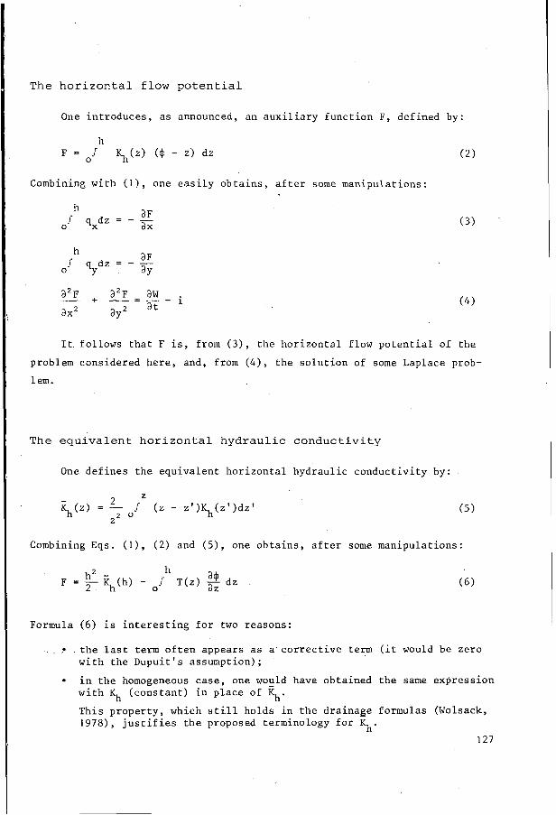
The horizontal flow potential

One introduces, as announced, an auxiliary function F, defined by:

h F = ol % ( z ) ($ - Z ) dz ( 2 )

Combining with ( I ) , one easily obtains, after some manipulations:

aF o/ qxdz = - - h

ax

aF J q d z = - - h

O Y aY

a2F

ax2 ay2 a% aw i + - = - - __

at ( 4 )

It. follows that F is, from ( 3 ) , the horizontal flow potential of the

problem considered here, and, from ( 4 ) , the solution of some Laplace prob-

lem.

The equivalent horizontal hydraulic conductivity

One defines the equivalent horizontal hydraulic conductivity by:

Combining Eqs. ( I ) , (2) and ( 5 ) , one obtains, after some manipulations:

Formula ( 6 ) is interesting for two reasons:

. the last term often appears as a corrective term (it would be zero with the Dupuit's assumption);

in the homogeneous case, one would have obtained the same expression with Kh (constant) in place of This property, which still holds in the drainage formulas (Wolsack, 1978) , justifies the proposed terminology for

Kh'

127 Kh.

The gene ra l method f o r o b t a i n i n g d ra inage formulas c o n s i s t s i n eva lua t -

i n g F by two means ( d i r e c t l y from ( 2 ) o r ( 6 ) , and by so lv ing ( 4 ) under t h e

a p p r o p r i a t e boundary c o n d i t i o n s ) and t o equal t h e expres s ions d e r i v e d .

An e x a c t equat ion for t h e pumping t e s t

F i e l d experiments show t h a t , w i th c e r t a i n c a r e (Guyon, 1971), one can

o b t a i n , f o r water t a b l e s t y p i c a l of land d ra inage problems, a q u a s i s t eady

s t a t e when pumping a t a ,low d i scha rge . The r a d i u s of i n f l u e n c e i s t h e r e f o r e

o f about s e v e r a l me te r s , which cor responds t o t h e purpose of land d ra inage

(F ig .1 ) . ,

.h

-

T

i 1 I I I

1 1 I I I 1 1 1 I 1

impervious layer I 1

ra m r

F i g . I. F u z z y ' p e n e t r a t i n g well.

Denoting r t h e d i s t a n c e t o t h e w e l l a x i s ( t h e w e l

pe rv ious l a y e r ) , ( 4 ) y i e l d s , i n s t eady s ta te , and wi th

a t t a i n i n g t h e im-

no i n f i l t r a t i o n :

I d dF - - ( r - ) = O r d r d r

128

( 7 )

The boundary conditions on the well are:

@ = z d < z < h (r ) P

4 = d O < z < d

Integrating (7) with ( 3 ) and ( 8 ) , one obtains, denoting Q the pumping di schar ge :

A

P

r Q - In (-) = F (TA) - F (r 2II r P

Evaluating F(rA) from (6) and F(r ) from ( Z ) , one finally obtains: P

The last term of (9) appears as a corrective term, as smaller as r A is

greater. One developes thereafter some evaluation procedures for this term.

Evaluating the corrective term in a homogeneous and isotropic soil

I n an homogeneous and isotropic soil, formula (9) yields:

A h~ a+ II P

r=rA r a In (F) = (hi - d2) K - 2 K o / z dz l

a+ K - can be estimated as follows (from (I)): aZ dh

O c K - 34 (r z ) = lqz l (rA,Z) < ( q z ( (rA,hA) = (qr( (rA,hA) (rA) az a'

One has, too:

(10)

(slope of the f ree surface with the Dupuit 's assumption)

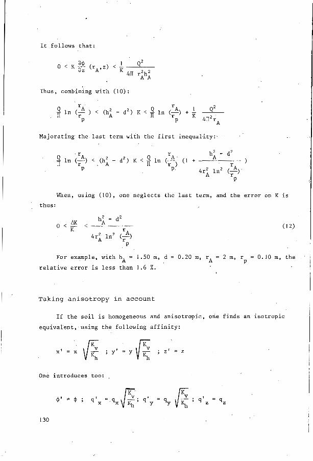
Majorat ing t h e l a s t term with t h e f i r s t i n e q u a l i t y :

When, using ( I O ) , one neg lec t s t h e l as t t e r m , and the e r r o r on K i s

thus:

h i - d2

rA 4 r i In2 (y>

AK o < - < K

P I

For example, w i th hA = 1.50 m, d = 0.20 m, rA = 2 m, r = 0.10 m y the P

r e l a t i v e e r r o r i s l e s s than 1 .6 %.

I ’ Taking anisotropy in account

I I f t h e s o i l i s homogeneous and a n i s o t r o p i c , one f i n d s an i s o t r o p i c

equ iva len t , using t h e fol lowing a f f i n i t y :

One in t roduces too:

130

One. e a s i l y v e r f i e s t h a t ( 1 ) can be w r i t t e n i n ( + I , 9 ' ) and ( x ' , y ' , z ' )

a s f o r a n homogeneous and i s o t r o p i c s o i l of hydrau l i c conduc t iv i ty K . V

One can thus copy ( 1 1 ) w i th :

K + K v , ; Q + Q - ; KV r A + r A & ;, rp + rp & E ; , .

One o b t a i n s a f t e r re-arrangement:

I f E;, i s es t imated by t h e approximate formuIa:.

Then t h e r e l a t i v e e r r o r becomes :

E;, A - Kv

hk - d2 -

r % o < - - <

I$, 4 r i I n 2 (F) P

The r e l a t i v e e r r o r i s dec reas ing when K i s i n c r e a s i n g , which is nor- V

m a l because, a t t h e l i m i t , f o r K i n f i n i t e , t h e Dupu i t ' s assumption (hydro-

s t a t i c p r e s s u r e d i s t r i b u t i o n ) i s s t r i c t l y v e r i f i e d : V

Tak ing h e t e r o g e n e i t y i n a c c o u n t

One has now t o e v a l u a t e t h e e r r o r appear ing when neg lec t ing the cor rec-

t i v e term of ( 9 ) , say:

This e v a l u a t i o n w i l l be q u a l i t a t i v e , and based on observ ing t h e evolu-

t i o n of t h e c o r r e c t i v e t e r m , when pass ing from a r e fe rence homogeneous case

t o t h e a c t u a l heterogeneous case. I n a homogeneous s o i l , t h e e q u i p o t e n t i a l s

have t h e shape shown i n Fig.2A.

131

A B . C TI cpc: I

I

D

! ! ! -

highly

permeable I --- permeable poorly i[---

A : Kh(z) constant

C: Kh(z) increasing

B: $ ( z ) decreasing

D: layered soil (example)

F i g . 2. Equipotentials in an heterogeneous s o i l .

If the hydraulic; conductivity increases with depth, the streamlines are

deviated downwards and the equipotentials are less vertical, which increases

the modulus of the corrective term (Fig.2B).

If the hydraulic conductivity decreases with depth, the streamlines are deviated upwards, which makes the equipotentials more vertical and the modu-

lus of the corrective term smaller (without probably changing its sign)

(Fig.2.C).

In the case of a non-monotonous variation, one obtains a combination

of both effects (Fig.2D).

The well and piezometer method

According to the preceding results, one can conclude that the corrective

term of (9) is generally negligible, except:

5l Kv

- when the anisotropy ratio - is very high;

- or when there is a very permeable layer at some depth.

132

I n . b o t h c a s e s , which can be guessed by t h e s o i l s c i e n t i s t (and eventu-

ally v e r i f i e d wi th t h e Verg ière method (Bour r i e r , 1965)), it i s necessary t o

ho ld a p a r t i c u l a r s tudy . 1

I n t h e gene ra l ca se , t h e pumping tes t i s conducted i n o r d e r t o e s t i m a t e

% wi th t h e formula ( 9 ) , s i m p l i f i e d as fo l lows:

F i r s t , one must remind t h a t t h e r e i s need f o r < ( z ) a t one, two o r t h r e e

d i f f e r e n t l e v e l s , which l eads t o one, two o r t h r e e success ive quas i s t eady

s t a t e s .

1'0 R

F i g . 3. Three ZeveZs in a pumping t e s t .

Fig . 3 i l l u s t r a t e s t h e th ree - l eve l t es t ; t h e formulas provid ing the t h r e e

v a l u e s of a r e r e s p e c t i v e l y , from (16) : Kh

133

For the two-level test, one makes. steps 2 and 3 only. For the one-level test, one makes step 3 only.

Conclusion

Estimating the soil hydraulic conductivity is a major problem of pre-

drainage studies. In homogeneous cases, the "well and piezometer method" 1

proved to be the most relevant method, according to french experience. -The

adaptation to hetierogeneous cases demands answer to two questions:

- how to describe heterogeneous hydraulic conductivity? - is it possible to estimate the parameters used

in this description?

The first question has been given an answer in Wolsack (1978) , through

the introduction of the concept of "equivalent horizontal hydraulic conducti-

vity", which proved to be well'adapted to some drainage calculations.

The second question was answered in this paper, through an adaptation

of the "well and piezometer method". The general procedure remains identical,

but, because the equivalent horizontal hydraulic conductivity is a function of elevation, more measurements have to be done, with different water.levels

in the well.

134

R e f erence s

BOURRIER, J. 1965. La mesure des caractéristiques hydrodynamiques des sols par la méthode Vergigre; Bull. Tech. de Génie Rural No.73, 96 pages.

GUYON, G. 1964. Considérations sur l'hydraulique des nappes de drainage par canalisations souterraines; Bull. Tech. Génie Rural No.65, 45 p. + annexes.

GWON, G., THIRRIOT, C. 1967. Sur le drainage des nappes perchées en période de tarissement; C.R. Acad. Sci. Paris, t. 264, série A, 43-46.

GUYON, G. 1968. Le drainage des nappes perchées; ENGREF, Paris.42 p.+annexes.. GWON, G.

du rabattement de nappe en vue des calculs du drainage; Bull. Tech. Génie Rural No.110, 29-49.

un écoulement B surface libre avec surface de suintement; C.R. Acad.

1971. Mesure de la conductivité hydraulique d'un s o l par la méthode

TCHARNYI, I.A. 1951. Démonstration rigoureuse de la formule de Dupuit pour

Sci. URSS 6.

ENGREF Paris.

sols hétérogènes et anisotropes, Bull. BRGM (2), 111, 2.

Houille Blanche 3, 385-388.

WOLSACK, J. 1976. Hydraulique souterraine 2. 1n:Cours d'hydraul

WOLSACK, J. 1978. Quelques extensions de la théorie du drainage

ZAOUI, J. 1964. Les écoúlements en milieu poreux,et l'hypothèse

que générale,

aux cas de

de Dupuit;

135

Paper 1.05

PRE-DRAINAGE RESEARCH IN LAND CONSOLIDATION AREAS

W.van der Meer, Government Service for Land and Water Use, Groningen, The Nether Zands

Summary I f , i n case of re-al lotment , s u b s o i l drainage i s . i n c l u d e d i n the p l an of pro v i s i o n s , pre-drainage r e sea rch i s gene ra l ly made t o determine t h e i n t e n s i t y o f drainage r equ i r ed . Apart from t h e o b j e c t i o n of too a u n i v e r s a l l y app l i ed measuring and c a l c u l a t i n g technique regarding t h e Hooghoudt s t a t i o n a r y flow p r i n c i p l e , an inc reas ing number of ob jec t ions have been r a i s e d f o r t he l a s t y e a r s t o t h e c u r r e n t method of pre-drainage r e sea rch by means of t h e Auger h o l e method. These ob jec t ions are gene ra l ly d i r e c t e d a t t he very high c o s t s of t h i s labour i n t e n s i v e i n v e s t i g a t i o n and t h e use fu lness of t h e r e s u l t acquired. P a r t i c u l a r l y t h e range i n p e r m e a b i l i t i e s measured i n a (systematic i n v e s t i g a t i o n , causes problems. An i n t e n s i f i c a t i o n of t h e i n v e s t i g a t i o n u s u a l l y produces no b e t t e r information.

During t h e l a s t few y e a r s , however, favourable experiences have been gained w i t h r e sea rch more focussed on t h e hydrological q u a l i t i e s of t h e p r o f i l e .

t i o n between p r o f i l e s t r u c t u r e and t h e d r a i n d i s t a n c e c a l c u l a t e d by means 1

of t h e Auger h o l e method. A s t r o n g cu t down of t h e measuring programme i s ob ta ined by s o i l type c l a s s i f i c a t i o n based on hydro log ica l q u a l i t i e s , by making permeabi l i ty measurements i n r e l e v a n t p r o f i l e types, and by next ex- t r a p o l a t i n g t h e information acquired from a number of t r i a l blocks. Dependent on t h e required r e l i a b i l i t y of t h e conclusion t h e number of d r a i n d i s t a n c e c a l c u l a t i o n s can be determined s t a t i s t i c a l l y . The number of permeab- i l i t y measurements can be reduced by h a l f , i f a c l a s s i f i c a t i o n i n p r o f i l e t ypes i s used and by even more, i f t h e borings are c a r e f u l l y d i s t r i b u t e d over t h e d i f f e r e n t p r o f i l e t ypes . A l l t h i s on cond i t ion t h a t t h e r e is no re- l a t i o n between permeabi l i ty and t h e depth of t h e impermeable l a y e r . A f u r t h e r r educ t ion of t h e number of pe rmeab i l i t y measurements can be reached by extend i n g t h e boring depth t o a t least 1.50 m i n t h e s o i l survey and by e s t ima t ing t h e pe rmeab i l i t y of t h e d i f f e r e n t p r o f i l e l a y e r s , a f t e r experience and in s igh have been gained with (gauge) measurements i n r e l e v a n t p r o f i l e l a y e r s . The e x t r a c o s t s of such a d e t a i l e d survey are, i n every r e s p e c t , accep tab le i n view of a r e s t r i c t i o n of t h e l a te r pre-drainage r e sea rch . The g r e a t i n t e n s i t y of t h e p r o f i l e d e s c r i p t i o n s i n t h e s o i l survey (one i n every 1-3 ha) makes a c l a s s i f i c a t i o n i n p r o f i l e types p o s s i b l e , i n which a d d i t i o n a l measurements have been r e s t r i c t e d t o p a r t s of t h e drainage plan. It should be noted t h a t t h e g e n e r a l l y s t a t e d l i m i t a t i o n of pre-drainage r e sea rch only a p p l i e s t o measurements,but no t t o borings made t o determine t h e depth of t h e impermeabl l a y e r . Espec ia l ly i n t o t h i s matter a d d i t i o n a l i n v e s t i g a t i o n s must be made.

This r e p o r t mainly d e a l s w i th t h e approach t o and t h e form of pre-drainage r e s e a r c h based on t h e s t a r t i n g - p o i n t regarding s o i l maps. The recommendations have always been based on t h e r e l a t i o n between p r o f i l e s t r u c t u r e and d r a i n d i s t a n c e . I36

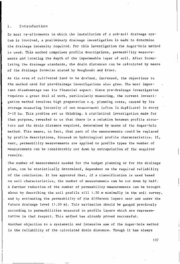
1 , Introduction

The number of measurements needed for the budget planning or for the drainage

plan, can be statistically determined, dependent on the required reliability

of the conclusion. It has appeared that, if a classification is used based

on soil characteristics, the number of measurements can be cut down by half,

A further reduction of the number of permeability measurements can be brought

about by describing the soil profile till 1.50 m minimally in the soil survey, and by estimating the permeability of the different layers near and under the ,

future drainage level (1.20 m). This estimation should be gauged previously

according to permeabilities measured in profile layers which are represen- tative in that respect. This method has already proved successful.

Another objection to a systematic and intensive use of the Auger-hole method

is the reliability of the calculated drain distance. Though it has always

,

In most re-allotments in which the installation of a sub-soil drainage sys-

tem is involved, a preliminary drainage investigation is made to determine

the drainage intensity required. For this investigation the Auger-hole method

is used. This method comprises profile descriptions, permeability measure-

ments and locating the depth of the impermeable layer of soil. After formu-

lating the drainage standards, the drain distances can be calculated by means

of the drainage formulas stated by Hooghoudt and Ernst.

As the area of cultivated land to be drained, increased, the objections to

the method used for pre-drainage investigations also grew: The most impor- .

tant disadvantage was its financial aspect. Since pre-drainage investigation

requires a great deal of work, particularly measuring, the current investi-

gation method involves high preparation c.q. planning costs, caused by its

average measuring intensity of one measurement (often in duplicate) in every

5-10 ha. This problem set us thinking. A statistical investigation made for

that purpose, revealed to us that there is a relation between profile struc-

ture and the drain distance required, determined by means of the Auger-hole

method. This means, in fact, that part of the measurements could be replaced

by profile descriptions, focused on hydrological profile characteristics. If, next, permeability measurements are applied to profile types the number of

measurements can be considerably cut down by extrapolation of the acquired

results.

1 137

I

been assumed that the right drain distance can be calculated by means of the

Auger-hole method, investigations have shown a great range in permeabilities

within the same soil structure. A more elaborate observation system of one

in every 10 ha, to one in every 3 ha and even one in every 16 m , did not, however, give any better information about the exact permeability.

A general application of *the Auger-hole method has formerly led to the deve-

lopment of quick and clear measuring and calculation techniques. The routine

character that resulted from the application of these techniques has led too a universal application of the Hooghoudt and Ernst formulas for stationary

state flow. This,objection has been raised time and again for the last few

years in the resumed discussion about agricultural discharge standards and

drainage criteria. New directions are to be expected fairly soon concerning

aspects such as: drainage criteria (differentiation based on trafficability

and cultivation requirements, water storage and drain depth), formulas and

nomogrames (the influence of drain length and flow resistence on the drain

p'ipe diameter).

The costs and discontent at the quality and usefulness of the acquired resul

have led us to take a new course for the last few years. As the present methl

of pre-drainage investigation differ a great deal in every district, a unifo

approach is needed using new developments and meeting the above objections.

Hereto recommendations are mentioned in this report. Distinction has been mal

according to the purpose of the investigation, namely whether it has been mal for budget purposes or for the drainage plan.

The Auger-hole,method haS.been maintained as point of departure, but the

accent has been shifted to soil characteristics.

2

2. Summary of some relevant investigation results

2.1 Relationship between profile structure and the drain distance required

If pre-drainage investigation aims at extrapolation of permeability factors

by means of soil characteristics, it must be proved that there is a relation between these soil characteristics and the drain distance calculated from thc

Auger-hole method. This had been worked out in the re-allotment of "Slochte-

138

ren". With t h e h e l p of p r o f i l e d e s c r i p t i o n s a d i v i s i o n w a s made . in s o i l

( h y d r o l o g i c a l ) ' u n i t s , i n which t h e p r o f i l e s t r u c t u r e round and beneath t h e

f u t u r e d r a i n l e v e l (about 1.20 m) has been taken f u l l account o f .

For sandy s o i l s , a simple c l a s s i f i c a t i o n i s p o s s i b l e based on t h e depth of

t h e impermeable l a y e r and loam percentage ,so t h a t a s a t i s f a c t o r y c o r r e l a t i o n

i s obta ined between t h e s e c h a r a c t e r i s t i c s and t h e average d r a i n d i s t a n c e .

I n some cases a c l a s s i f i c a t i o n accord ing t o coarseness of t h e sand i s a l s o

cons idered u s e f u l . The d i f f e r e n c e s i n d r a i n d i s t a n c e appeared t o be , ' i n most

c a s e s , s t a t i s t i c a l l y r e l i a b l e . V a r i a t i o n i n d r a i n d i s t a n c e w i t h i n t h e p r o f i l e

t ypes formed, g e n e r a l l y appeared t o be i n l i n e wi th t h a t which occurs i n ,

homogeneous areas cover ing 6 ha. This s u r f a c e i s considered t o be t h e small-

e s t u n i t which s t i l l g e t s a s e p a r a t e d r a i n d i s t ance .

For sand s o i l s i n t h e land conso l ida t ion a r e a of "Slochteren" t h e r e s u l t s of

t h e sys t ema t i c pre-drainage i n v e s t i g a t i o n have been worked o u t a s fo l lows .

A c o r r e l a t i o n between loam percentage and d r a i n d i s t a n c e by d i f f e r e n t depth

of t h e impervious l a y e r i s shown i n Table I . The d r a i n d i s t a n c e has been c a l -

c u l a t e d by means of t h e Hooghoudt formulae f o r s t eady- s t a t e flow; t h e K-

v a l u e s were measured by means of t h e Auger-hole method. Loam percentage is

g%en i n t h r e e c l a s s e s : 1:5-10 %; 2:lO-18 %; and 3:18-50 %. These c l a s s e s

w e r e e s t ima ted by t h e p r o f i l e d e s c r i p t i o n s . The loam percentage of t h e l a y e r s

around and beneath d r a i n l e v e l are r e l e v a n t . ,

The d i f f e r e n c e i n d r a i n d i s t a n c e s have been proved t o be s i g n i f i c a n t .

TABLE I .

Depth of the Number of Average Standard deviation i n impervious Loam class calculations drain layer below distance surface (n) (X ) m z of x

~

1.00 - 1 .20 m . I 15 14. I 5 . 5 39

1.00 - 1 .20 m 2 12 13.2 . 5 . 5 42

1.00 - 1 .20 m 3 4 9 . 8 6 . 4 65

1 . 2 0 - 1 . 6 0 m I 44 22 .2 8 . 2 37

1 .20 - 1 .60 m 2 , 53 17.2 8. I 46

1 .20 - 1 .60 m ' 3 4 13.2 2 . 6 20

1 . 6 0 - 2 . 5 0 m 1 114 33. I 16 .3 31

1 .60 - 2 .50 m 2 93 24.5 7 . 7 32

1 .60 - 2 .50 m 3 9 19.6 7 . I 36

139

For the peat-soils, in which peaty material is found at drain level, it ap-

peared to be impossible to make such a division in profile types that it led

to a correlation with the drain distance. Its variation was, however,'hardly

greater than the variation in drain distance in homogeneous units of peat

soils of at least 6 ha. Experiences elsewhere have proved, however, that if

a classification is made according to the types of peat, a differentiation

in drain distance will certainly appear.

In clay soils the permeability is influenced by its lutum percentage, its

degree of'stratification, its stage of physical maturation and the local

occurrence of a particularly permeable structure ("short clay"). A classi-

fication in profile types based on these characteristics is to be preferred

for very precise drain distance calculations.

From investigations in the re-allotment area of "Harkstede" it has appeared

that permeability measurements can be largely replaced by estimation. In the soil survey of the area the profile has been described till 1.50 m. In this description the permeability of each profile layer has been estimated

separately after experience and insight had been gained with preliminary

measurements in representative profile layers.

After a classification of the area according to relevant profile types and

estimated permeability, additional permeability measurements were taken and

deeper borings were made to ldcate the depth of the impermeable layer. A

comparison of the drain distance calculated for every separate hydraulic

profile type from measured permeabilities with that calculated from estima-

ted permeabilities revealed nearly the same results.

Table 2 shows the range in K-values in two different soil types and gives

the average K-value (measured and estimated) for drain distance calcu-

lations.

2.2 Approach to the number of drain distance observations

The "Slochteren" investigation also aimed at figuring the number of drain

distance observations necessary for the final drainage plan only, or for

budgeting. To this end formulas have been deduced, which have been graphi-

cally worked out in Figures I and 2.

140

TABLE 2.

Range and fkequency of t h e K-value i n m/day Depth of t h e Medium-

impervious 0.10 0.20 0.40 0.60 0.80 1.20 v a l u e of S o i l t y p e

l a y e r K <o. I O t o t o t o t o t o t o > I .80 K (mlday) - - 0.20 0.40 0.60 0.80 1.20 1.80

pea ty s o i l < - 1.20 m M* 20 9 13 2 5 2 1 - 0.17, m/d w i t h sha l low below above podzol s u r f a c e E 50 136 57 17 3 4 5 - 0.16 m/d

sand s o i l above M 5 4 6 5 2 1 1 - 0.30 m/d w i t h po'dzol below M 2 4 9 - 3 1 - 1 4 0.35 m/d

1.80 m above E 20 132 169 80 18 6 I O 5 0.28 m/d

below E I O 69 172 107 48 19 9 6 0.36 m/d

c h a r a c t e r -

i s t i c s

* M = measured E = estimated

Though from these figures the number of permeability measurements for every

separate profile type can be calculated, it may not be concluded that, as

the number of separate profile types increases, the total number of measure-

ments to be taken will increase in proportion. Usually the drain distance

of a profile type can be deduced from another profile type. Soil types with,

for instance, the same loam percentage differ, in a hydrological respect,

exclusively in the depth of the impermeable layer.

Permeability measurements are, therefore, only wanted for soils with a dif-

ferent loam percentage. Thus the total number of measurements can be consid-

erably cut down. However,.there must be no relation between the permeability

of the soil and the depth of the impermeable layer.

Figures 1 and 2 are based on the formula:

. 100 tn-l Sx v = - . - /ÌT x

in which V = the maximum deviation (in X ) allowed between the calculated

and the factual average drain distance

Sx

x n = number of observations,

tn-l = measure of excentricity dependent on the number of observations

= standard deviation from the original classification

= the average drain distance in every profile type -

,

(n-I) and of CY. (measure of unreliability).

In this connection it is impossible to cut down the number of borings for

the depth of the impermeable layer. If nothing is known of the value =- 100

in Figures 1 and 2, it may be necessary to estimate this value by means of

a number of permeability measurements made previously.

To determine the number of measurements necessary for budgetting, the drain- age costs are assumed to be proportionate to the length of the drain pipes

to be laid. Figures 1 and 2 can be used again here.

From the investigations at "Slochteren" it has appeared that, if a classifi-

cation in profile types is used, the total number of permeability'measure-

ments (from Figures 1 and 2) can be reduced by about one half as compared

with the situation in which no use is made of this classification. If the

number of measurements were not distributed over the profile types in propor-

sx X

142

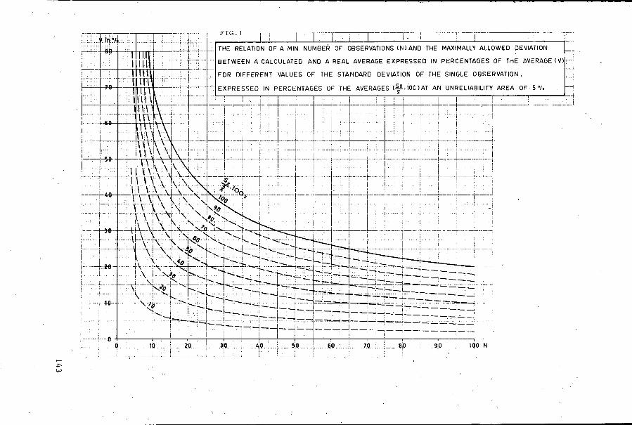
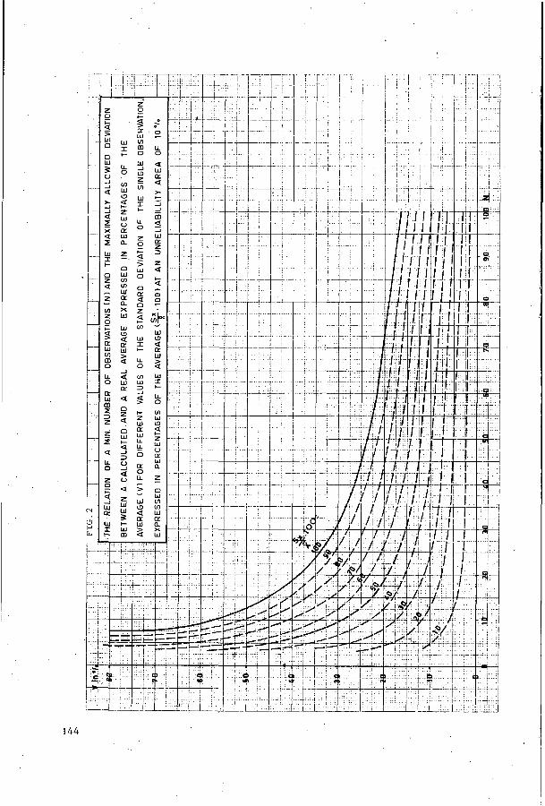
N

144

t i o n t o t h e r e l e v a n t a r e a , bu t were based on an optimum d i s t r i b u t on, t h e

t o t a l number of obse rva t ions would be reduced by about anothe? q u a r t e r .

I f t h e s o i l has been mapped o u t t o a depth of a t l e a s t 1.50 m with an es t i -

mation of t h e permeabi l i ty f a c t o r , i n most cases measurements w i l l be ha rd ly

necessary t o determine t h e budget. Nevertheless , t o o b t a i n a broad survey of

t h e depth of t h e impermeable l a y e r , i n o rde r t o c a l c u l a t e an average d r a i n

d i s t a n c e , s t i l l deeper borings w i l l be necessary.

3 . The need of a pre-drainage investigation

Once i t has been decided t h a t sub-soi l d ra inage w i l l be included i n t h e . p l a n

of p rov i s ions of a land conso l ida t ion area, the ques t ion arises t o what ex-

t e n t pre-drainage i n v e s t i g a t i o n w i l l be necessary. This depends on t h e in fo r -

mation a v a i l a b l e about t he cond i t ion of t he s o i l ( i t s degree of homogeneity),

t h e deeper s u b s o i l (deeper borings,’ geo log ica l maps) and the development p l an

i t s e l f .

Pre-drainage r e sea rch by means of t h e Auger-hole method is l e s s s u i t a b l e f o r

well-permeating sandy s o i l s i n which g r e a t d r a i n d i s t a n c e s a r e t o be expec-

t e d o r when drainage i s used i n s t e a d of d i t c h e s by f i e l d enlargement. I n

a r e a s with a very homogeneous s o i l ( p a r t i c u l a r l y with r e spec t t o t h e sub-

s o i l ) a simple f i e l d r e sea rch w i l l gene ra l ly succeed. I f f u r t h e r i n v e s t i g a t i o n

i s r equ i r ed , i t s form and e x t e n t w i l l be determined by t h e a v a i l a b i l i t y of

s o i l maps. Various p o s s i b i l i t i e s w i l l be d e a l t with i n the next s e c t i o n . .

4. Soil type information and investigation method

4.1 If a soil map is available

The s o i l map of a land conso l ida t ion area, e i t h e r rough ( s c a l e 1:50,000) o r

more d e t a i l e d ( s c a l e 1:10/15/25,000) w i l l be made i n t h e p repa ra t ion phase

and provides a s o i l c l a s s i f i c a t i o n based on t h e p r o f i l e s t r u c t u r e t o a depth

of 0.80 m. Although t h e bo r ing depth w a s gene ra l ly 1.20 m, t h e s o i l map does

n o t always supply information about t h e s o i l p r o f i l e deeper than 0.80 m ;

on ly i f a s u b s o i l map o r a sand depth map i s made, we can o b t a i n more in fo r -

mation on t h i s matter.

145

By an i n t e r p r e t a t i o n of t h e s o i l types due t o hydrau l i c c h a r a c t e r i s t i c s of

t h e s u b s o i l , t h e s o i l map can be more o r l e s s reduced t o a (rough) c l a s s i f i -

c a t i o n i n p r o f i l e types.

When planning t h e c o s t s of sub-soi l drainage i t i s important t o know the

t o t a l l eng th of d r a i n pipes and, i n a lesser degree, t o know the d i f f e r e n -

t i a t i o n i n d r a i n d i s t a n c e s .

A r educ t ion of t h e s o i l map t o a number of p r o f i l e types w i l l o f t e n s t i l l

supply a vague and incomplete p i c t u r e , p a r t i c u l a r l y as f o r t h e depth of t he

impermeable l a y e r . It i s , t h e r e f o r e , d e s i r a b l e t o have borings made t o maxi-

mum 2 o r 4 m o r , t o put i t more g e n e r a l l y , t i l l about 1 /8 of the d r a i n d i s -

t ance t o be expected. The number of borings and i t s d i s t r i b u t i o n over t he

a r e a i s dependent on t h e degree i n which (hydrological) p r o f i l e types have

been d i s t ingu i shed and marked o f f . The s c a l e of t h e map and pe r sona l in-

s i g h t w i l l a l s o play a p a r t i n t h i s matter.

I t must a l s o be taken i n t o account, t h a t during the second phase (drainage

p l a n ) , a f t e r re-al lotment has been pu t t o t h e vo te , a more sys t ema t i c inves-

t i g a t i o n i n t o t h e depth of t h e impermeable l a y e r can t ake p l ace .

When those borings a r e made, a t t e n t i o n should a l s o be paid t o the p r o f i l e

c h a r a c t e r i s t i c s . More r e sea rch f o r t h e f i r s t phase (budget) can then be

r e s t r i c t e d t o one o r more t r i a l blocks f o r every p r o f i l e type. I n every t r i a l

block a few d r a i n d i s t a n c e s w i l l be c a l c u l a t e d , a f t e r which t h e average d r a i n

d i s t a n c e can be ex t r apo la t ed i n p ropor t ion t o the s u r f a c e of each p r o f i l e

type. Dependent on t h e required r e l i a b i l i t y of t h e conclusion, t h e t o t a l num-

b e r of obse rva t ions can be approached s t a t i s t i c a l l y (Sect ion 2 ) .

To make a drainage p l a n which i n d i c a t e s and marks o f f t h e h i f f e r e n c e s i n

d r a i n d i s t a n c e s as c l e a r l y as p o s s i b l e , t he preceding phase has a l r eady pro-

vided a f i r m base.

Obscur i t i e s i n t h e (rough) p r o f i l e type c l a s s i f i c a t i o n , e s p e c i a l l y i n the

less homogeneous areas, have s t i l l been i n s u f f i c i e n t l y resolved by the ex-

t r a information from t h e a d d i t i o n a l borings and measurements. A c l o s e r in-

v e s t i g a t i o n must, t h e r e f o r e , be focussed p a r t i c u l a r l y on the depth of t he

impermeable l a y e r , while permeabi l i ty measurements should io l low ' af terwards.

The number of measurements ( inc lud ing those from t h e f i r s t phase) and t h e i r

146

d i s t r i b u t i o n over t h e p r o f i l e types can, i f r equ i r ed , be c a l c u l a t e d s ta t is-

t i c a l l y , and i s h i g h l y dependent on t h e number of d i f f e r e n t p r o f i l e types .

I n a gene ra l s ense i t must be noted t h a t deeper bor ings are s i g n i f i c a n t es-

p e c i a l l y i n sandy s o i l s . Clay s o i l s are d i f f e r e n t because, on account of

t h e i r r e l a t i v e l y low pe rmeab i l i t y , a de t e rmina t ion of t h e r i g h t depth of t h e

impermeable l a y e r has l e s s i n f l u e n c e on t h e d r a i n d i s t a n c e i n t h i s t ype of

s o i l .

I f t h e r e i s no d e t a i l e d s o i l map o r i f an e x i s t i n g s o i l map does no t g i v e

any informat ion about t h e l a y e r s , deeper than 0.80 m, a q u i t e d i f f e r e n t ap-

proach t o pre-drainage r e sea rch may be chosen i n t h e f i r s t and second phase.

I n t h e f i r s t phase d r a i n d i s t a n c e obse rva t ions have been executed by means

of sys t ema t i c network of bo r ings made wi th a average i n t e n s i t y of one bor ing

i n every 30 t o 50 ha .

A f t e r t h e d a t a have been worked ou t and s o i l d a t a have been i n t e r p r e t e d , ad-

d i t i o n a l i n v e s t i g a t i o n f o r t h e d ra inage p l a n can be d i r e c t e d a t a more accu-

r a t e marking o u t of d i f f e r e n t d r a i n d i s t a n c e s e c t i o n s . Such an approach

seems, t h e r e f o r e , t o be only s i g n i f i c a n t f o r areas wi th a more homogeneous

s o i l . I n heterogenous areas, t h e number of necessary obse rva t ions w i l l rap-

i d l y inc rease .

4 . 2 If a s o i l m a p is still to be made

The advantage of t h i s s i t u a t i o n i s , t h a t t h e s o i l survey program can be ad-

ap ted t o t h e f u t u r e pre-drainage r e sea rch . The e x t r a c o s t s involved are l i m -

i t e d , i n comparison wi th t h e t o t a l costs of t h e usua l survey and cer ta in ly a c c e p t a b l e i n view of an economization of t h e pre-drainage r e sea rch t o be

made la te r on.

The ' i t ems of survey ex tens ion are:

a )

b)

Boring depth and p r o f i l e d e s c r i p t i o n should be extended t o a depth of a t least 1.50 m.

An e s t i m a t i o n of t h e pe rmeab i l i t y of every d i f f e r e n t p r o f i l e l a y e r (be- yond 0.50 m) from s o i l c h a r a c t e r i s t i c s . Prev ious t o t h e survey a rough i n v e n t a r i s a t i o n should be ?de of t h e most r e l e v a n t p r o f i l e l a y e r s , t h e pe rmeab i l i t y of which should be measured by means of t h e Auger-hole method.

147

The results of these gauge measurements should be analysed very accura- tely in order to gain some insight into permeability determining charac- teristics of the soil profile. .

Although it is well-known that permeabilities measured in peaty soils may greatly differ, it has appeared from experience that the type of peat and its structure play an important role. Attention should be paid to this when surveying the soil. An estimation of the permeability will then lead to a better result than measuring.

c)

d) A part of the borings can be made to 2 or maximum 4 m. The intensity and depth of the borings depend A careful consideration of extra costs of surveying on the one hand and a limitation of a later additional investigation on the other is desirable. Sometimes it is enough to make deep borings in a number of section lines.

on drain distance to be expected.

From a profile type classification, a classification of (hydrological) pro-

file types can be made by an interpretation of the permeabilities estimated,

profile description and data about the depth of the impermeable layer.

Frequently there will not be enough information about the deeper subsoil,

which may be investigated separately, if necessary. Together with these

additional data sufficient material has been collected to make the budget for

the subsoil drainage plan. A comparison between measured and estimated per-

meability factors is also necessary at this stage.

The step to the second phase, the drainage plan, can be restricted after,the

previous elaborations. For a proper differentiation in drain distance and a

clear marking out of different distance sections, another number Ò f measure-

ments may be necessary and certainly a more or less daborate network of

deeper borings. No extra research is necessary in peaty soils and in profile types which represent a smaller area.

It should also be mentioned that a detailed differentiation in drain distance is not reasonable; a reduction to a restricted number of different distance

sections, therefore, is preferred.

148

R e f erences

I I

Government Service for Land and Water Use, Research Section: ,

Groningen: Relationship between soil profile and drain distance required in

Leeuwarden: Pre-drainage investigation in the land consolidation area of the land consolidation area of "Slochteren" (Bulletin 109, Sept. 1973).

"Wonseradeel-noord". (Aug. 1976).

ERNST, L.F. 1950. A new formula to calculate permeability by means of the Auger-hole method. T.N.O. Groningen.

HOOGHOUDT, S.B. 1940. Contribution to the knowledge of some physical quan- tities of the soil. Report Agricultural Research 46. Groningen.

MEER, W. v.d. and G. RUTTEN. 1976. Developments in the methods of pre-drain- age research in the province of Groningen applied to the re-allotment area of "Harkstede". Bulletin C.D. Istiboka.

land development projects. 5th meeting of the Drainage Contact Group, Government Service for Land and Water Use, Utrecht.

NAARDING, W.H. Various methods of pre-drainage research in the interest of

SOMEREN, C.L. v. 1975. Pre-drainage research by and for the Government Ser- vice for Land and Water Use. 138th meeting of Research Engineers. Government Service for Land and Water Use, Utrecht.

149