258

4. Family background, gender and cohor effect on schoolingdecisions

Javier Valbuena, University of Kent

259

Family background, gender and cohor effect on schoolingdecisions

Javier Valbuena, University of Kent

abstractIn this paper we use unique retrospective family background data from wave 13th of the British Household Panel Survey (BHPS) to analyze the relevance of family background, in particular parental education - separated for fathers and mothers -, and gender on differential educational achievement. We find parents’ education attainments to be strong predictors of the education of their offspring. In particular, maternal education is the main determinant on the decision of whether stay-on beyond compulsory education. Our results are robust to the inclusion of a large set of control variables, including household income.

Keywords: Educational attainment, schooling, early school leaving, education transmission JEL Classification: I21, I28, J11.

1. Introduction The relevance of education has risen considerably during the last decades in industrialized countries as we all understand that one of the most valuable resources of our societies is the education children obtain in our national education systems. The relevance of educational outcomes is now widely documented both at a macro-level and at a micro-level94. The direct implication of these facts is an increasing interest on the factors that affect educational decisions; especially taking into account that most part of the educational cost is public-financed or at least public expenditures are rising over time. Thus, in a context of scarce public resources, it is necessary to further understand the best channels to increase education in order to target public educational policies towards them. Following Haveman and Wolfe (1995), the main factors that determine the process of a child’s educational attainments are institutional factors (investment of public resources and determination of the cultural and socio-economic environment), parental factors (time and income devoted to children, decisions about schooling of a child, liquidity constraints and, most importantly, family background) and those decisions taken by the child which reflect their preferences. Intergenerational mobility or the transmission of socio-economic status across different generations is another important related-field of the literature about educational attainments. Educational economists are studying the extent of intergenerational educational mobility and how it evolves over time (Blanden et al. (2004), Checchi (2006) among others). In this framework, the key idea is the persistence of educational choices across generations, that is, the level of inheritance of some educational level per-se. This intergenerational transmission of education is determined by genetics (such as ability and motivation), cultural and socioeconomic factors (such as institutional framework, cultural belief, etc). Therefore, having information on educational attainments of contiguous generations of a representative sample of the population will offer some evidence on the intergenerational (im)mobility of educational choices. Given the importance

94 The expansion of education is associated with more economic growth and other macroeconomic aggregate outcomes and at individual level is strongly associated to an increase of labour market participation and/or employability, the higher income and other non-monetary outcomes i.e. health status, fertility (Currie and Moretti (2003)).

260

of education in determining future economic and social outcomes, evidence of a strong grade of persistence of education across generations will serve as a guide for policy makers to improve the situation of those individuals with low education, low income and low social standing. There is a vast literature covering the effects of the recent development and expansion of education expenditures. However, it is not yet clear who benefits the most from this process. Using U.S. data Cameron and Heckman (1998, 2001) conclude that the reduction of short term liquidity constraints do not affect schooling choices. Chevalier et al. (2003) using data from 20 countries provide evidence about the increase in the effect of parental education alongside the expansion of higher education. UK studies by Blanden and Machin (2004) and Blanden et al. (2005) show how the expansion of higher education has not reduced the gap in educational attainment between children of rich and poor parents. Overall it seems that equitable results are not achieved through higher public education expenditures. In this paper, we use retrospective family background data from Wave 13 of the British Household Panel Survey (BHPS) to investigate the relevance of family background, in particular parental education on educational attainment. The richness of the dataset allows us to use a large set of controls at early schooling ages relevant to those factors that the theoretical and empirical literature highlight as important in affecting educational outcomes. Alongside controls for individual characteristics, we exploit the longitudinal structure of the data to construct measures for family structure, attitudes towards education and parental wealth. Notably, we do not attempt to distinguish between the separate effects of “nature” (correlation between children’s education and those of their parents caused by genetic issues) and “nurture” (real productivity effect of parental schooling)95. Therefore, estimates will represent the gross effect of family background and genetic ability. Hence, the motivation for the present work is based upon the well documented idea of the important role that family background (such us parental education) plays in determining the educational process of individuals. The contribution of this paper aims to add to the existing literature by testing the economic hypothesis regarding the relationship(s) of parental background in child outcomes using unique information about family attributes. The plan of the paper is as follows. Section 2 outlines the existing literature. Section 3 describes the main features of the UK educational system. Section 4 discusses the theoretical model of educational attainment. In section 5 we explain the nature of the data used. Section 6 outlines the empirical approach, presents the main estimates and discusses the results of several robustness checks. The final section concludes.

2. literature review We find the first contributions to the study of the schooling determinants in the sociological literature in Boudon (1973), in which the final education attainment is decomposed into a finite series of stages. Mare (1980) extends that vision and considers that the result of a sequence of transitions in the educational system is the final educational attainment. More recently Cameron and Heckman (1998) introduced the concept of Educational Selectivity, criticising the schooling transition model proposed by Mare (1980). The main argument is based on the idea that coefficient estimates from schooling transition models that ignore components not observed by the econometrician but having influence on subsequent transitions (ability, motivation) are 95 Piketty (2000) points out the “poor” relevance of clearly distinguish both concepts; in a recent paper Cunha and Heckman (2007) analyze the complex interaction mechanisms of nature and nurture and they define as obsolete the separability of both concepts, e.g. “… the sharp distinction between acquired skills and ability featured in the early human capital literature is not tenable”.

261

dynamically biased, so there is a problem of dynamic selection bias. They characterize omitted variable bias and suggest an alternative choice-theoretic model for educational attainment that can be implemented empirically using an Ordered Choice Model. This contribution to the educational literature has become a seminal paper due to the inclusion of a very important issue in the field, the presence of endogeneity in the econometric models caused by unobserved individual heterogeneity. There is no way of talking about causality of the factors if we do not consider such endogeneity of the model; in what follows we briefly review the different approaches educational economists have adopted to overcome these issues.

2.1. Causal effects on Educational attainments Ermisch and Francesconi (2001) proposed the first important contribution following Cameron and Heckman (1998) trying to identify causal effects of family background on educational attainment using a theoretical model as a guide and data from the BHPS. They use an Ordered Logit Model and suggest that family background has causal effects on children educational attainment if and only if family background affects the cost of schooling. They report that only when family background affects the cost of schooling the relation between parents and children education represents a causal effect. Consequently, for individuals belonging to the group “poor parents” both family structure and parental education have a positive causal effect on children educational attainment96. There is another group of authors that have approached the identification of causal effects using Natural Experiments, so separating “nature” (genetic transmission) from “nurture” (productivity effects of parental education). Behrman and Rosenzweig (2002, 2005) use a sample of twin mothers in order to estimate causal effects of parental education on children’s education controlling for genetic bias and assortative mating97. The identification of causal effects has been solved adopting similar approaches by other authors like Sacerdote (2002), Plug (2004) and Plug and Vijverberg (2003, 2005). They use adoption as a natural experiment (children must be randomly assigned to adoptive families) understanding the estimate of parental education as causal effects given the non-relation between the biological and adoptive heritable endowments of the adoptees. A further approach to the identification of causal effects is the use of Social Experiments: institutional or social changes that create exogenous variation in the characteristics of interest (i.e. parental education) but which are not related to the unobserved determinant of the individual final outcome (i.e. educational attainment of the child). One of the most relevant contributions in the literature was provided by Black et al. (2005, 2008) in which they exploit a strong change in the educative legislation in Norway (1959) in order to obtain the identification of a pure causal effect of parental education on a children schooling using both cohort and territorial data under a difference in difference approach. Other similar studies are the ones by Chevalier et al. (2005) using data for UK (LFS) and by Oreopoulus (2006) using data for the US. They both use schooling reforms in order to create variations in parental education that are exogenous to other parental unobserved factors. They adopt an IV strategy to account for the endogeneity of parental schooling and family income. Their IV estimates contrast with previous results in the

96 They define “poor parents” as those ones not financially able to make transfers to their offspring, opposite to “rich parents” who do make financial transfers.97 Following Behrman and Rosenzweig (2002) by assortative mating we mean that “More schooled women in almost all societies marry more schooled men, and they thus marry more able man as well, given own ability-schooling correlations”. Therefore, mothers with higher levels of education may have children with greater academic and labour market performance due to intergenerational genetic transmission and assortative mating.

262

literature: they found that the strong effect of parental education becomes insignificant when including income measures. Therefore, permanent family income components turn out to be strong predictors of children educational attainment. Social Experiments have also been used to assist in the identification of causal effects. The emphasis of this approach has been to consider institutional changes as a source of variation in individual outcomes (i.e. the effect of time tracking). There are recent papers using this methodology, as the one by Bauer and Riphnahn (2006) for the Swiss population. They study the effect of the time of tracking on the educational attainment and on the relation between tracking and parental education using an Ordered Probit Model. They come to the conclusion that early tracking do increase the effect of high parental education on the child’s probability of reaching higher education. Another interesting paper is the one by Brunello and Checchi (2007). They perform a multi-country analysis using two different cohorts of individuals educated under the same institutional framework, allowing time variation related to the variation in schooling institutions over time. Their results contrast with the ones found by Bauer and Riphnahn (2006), as they find that the early tracking reinforces the negative effect of having an educated parent on the probability of dropping out. Finally, it is important to make some comments about a different methodological solution to the ones mentioned above, Structural Dynamic Choice Models. Under this framework the econometric model is recovered from a dynamic model for schooling choices solving a stochastic dynamic programming problem. The most interesting feature of these models is that they can generate counterfactual evidence, allowing for the possibility of ex-ante policy evaluation. The evidence reported from these models, that can be found among others in Eckstein and Wolpin (1999), Cameron and Heckman (2001), Keane and Wolpin (2001), Carneiro et al. (2002, 2003, 2003), Cameron and Taber (2004), Todd and Wolpin (2006), invalidate the results obtained using Natural and Social Experiments, at least for the US. Given that using this approach requires the existence of a long longitudinal micro-data set, which it is not available for European countries, it is difficult to establish whether the results are specific for the US.

2.2. Descriptive Studies on Educational Attainments The description of reality as a “snapshot” contributes to the empirical literature making use of more simple models, which are not directly aimed to obtain causal effects. Again the most relevant contributions are based on the theoretical model proposed by Cameron and Heckman (1998), an Ordered Choice Model. There are several papers that explicitly recover this model: a paper by Chevalier and Lanot (2002) in which they propose an estimation strategy separating the relative effect of financial situation from family characteristic effects in educational attainments. They estimate an Ordered Probit Model reporting the marginal benefits-marginal cost ratio of dropping off school at different ages by gender and cohort. They conclude there is a small effect of family income on educational decisions which is dominated by family background characteristics, mainly parental education. There are two papers, by Lauer (2002, 2003), in which a Multivariate Ordered Model is used to account for part of the dynamic selection bias. The 2003 paper performs a German-French comparison analyzing the effects of gender, family background and time-cohort on educational attainments. For that purpose she uses the German Socio-Economic Data Panel (GSOEP) and the Formation et Qualification Professionelles Survey for France. She reports a strong effect of both parental education and time-cohort variables on educational attainment, with the parental background effect much smaller for higher education. There are other studies based on Ordered Choice Models without making an explicit reference to the model developed by Cameron and Heckman (1998). An investigation about the

263

educational level of second generation of immigrants in Germany is carried out in a paper by Riphahn (2003). Using an Ordered Probit Model they found that there is an important educational gap between ethnic groups of the population. In a subsequent paper Bauer and Riphahn (2006) investigate the differences in educational attainment between Swiss natives and immigrants reporting the strongest effect of parental education on educational attainment for immigrants, and in particular for the second generation. Another interesting paper is the one by Dustmann (2004) in which he looks at correlations between parental characteristics and child schooling and earnings based on GSOEP data for German birth cohorts 1920 through 1966. He confirms that parental background affects child outcomes. There is also a recent working paper by Heineck and Riphahn (2007) which studies the temporal evolution of the effect of family background (and other explanatory variables such as demographic ones) on children’s education using a Multinomial Logit Model. The main findings of the study reflect a strong parental background effect on child educational attainment and no reduction of such an effect over the last decades in spite of massive public policy interventions and education reforms. Chevalier et al. (2003) conclude from their study of 20 countries that “the expansion of access to higher education has been concomitant with an increase in the effect of parental education”. The issue of intergenerational mobility raised the attention in the UK, which together with the United States is known for its low mobility, where Blanden et al. (2003), Blanden and Machin (2004) and Machin and Vignoles (2004) analysed changes in the correlation between parental relative income position and child educational outcomes. The key findings show that children of rich parents are the most benefited from the expansion of the higher education system and also that the gap between children coming from richer and poorer backgrounds has widened over time. Moreover, Galindo-Rueda and Vignoles (2005) conclude that relevance of parental background in educational attainment has increased alongside with a decrease of cognitive ability; that is educational outcomes have increased far more for those with low ability and high income background at the expenses of those with high ability and low income background (already suggested by Cameron and Heckman, 1998). A common pattern of the related literature presented here is the important role that family background, especially parental education, plays on determining the educational process of individuals.

3. uK education system: past, present and future98 Education in Britain is compulsory from the beginning of the school term after a child’s fifth birthday99 until the end of the academic year in which the child reaches the age of 16 (11 years of compulsory schooling)100. Mainly children attend primary schoolfrom the age of 5 to 11 (Key stage 1 and Key stage 2), then secondary school from the age of 11 to 16 (Key stage 3 and Key stage 4). At the end of compulsory schooling, students take GCSE examinations (General Certificate of Secondary Education) in a range of subjects. Once students have completed compulsory education they have the opportunity to choose between the academic or vocational stream. The next stage for students pursuing academic qualifications is the Advanced level of the General Certificate of Education (A-levels). That is, after GCSEs students take two further years of study following between two and four subjects101; results for A-levels exams are usually obtained

98 We refer to England, Wales and Northern Ireland.99 Nowadays the single entry point system is becoming increasingly popular; under this system all children must start school in September of the academic year in which they turn 5. 100 Before 1972 the minimum school leaving age was 15.101 In 1987 AS-levels were introduced; they are designed to occupy half of the teaching and study time of an A-level.

264

at the age of 18102. Beyond the age of 18 education takes place in universities, undergraduate degrees normally take 3 years and are usually completed when the person is aged 21-22. On the other hand students more vocationally oriented go on to Further Education Colleges resulting in higher vocational qualifications. Most schools in Britain are maintained by their Local Authority and could be described as comprehensive; therefore most children attend those schools that cater for all abilities in contrast to grammar and public schools103. Indeed, the private sector is small accounting for about 7 per cent of schools (Challen, Machin and McNally, 2008).

3.1. Major changes in the schooling system During the 1960’s and 1970’s the practice of separating children into different school types based on ability (children had to take an exam at the age of 11) was phased out. There are a small number of Local Education Authorities (LEAs) that retain the system but they are not representative of the population as a whole; in Northern Ireland the system is still in use. The effects of attending selective schools are difficult to identify and interpret given the problems of selection bias (i.e. non-random assignment of students) and since they operate through different channels (i.e. school resources). Alongside concerns about education inequality, since the 1980’s successive governments have introduced reforms in an attempt to improve the poor and falling standards of UK education. We briefly comment on the most important ones. In 1988 (Education Reform Act – 1988) a reform of the examination system at the end of compulsory schooling was undertaken; GCSEs replaced the GCE O-level system104. The key change of this reform was the conversion of a rationed education system (number of O-level passes in a given year were rationed) into one where “a priori” everyone could pass a GCSE (Blanden, Gregg and Machin 2005). A further modification concerned changes in the method of assessment: The GCE O-level system was based purely on exams; whereas the GCSE system involves a substantial coursework component105. The introduction of GCSEs was also accompanied by reforms aimed at increasing parental choice and improving the information available to parents about the effectiveness of schools. Several changes in educational participation and attainment appear to be linked to the introduction of the GCSEs and reform of the exam system. McNally (2005) identifies the percentage of students achieving five or more grades at A*-C in the O level/GCSE examinations between 1970’s and the present to have risen considerably. Blanden et al. (2005) reports the rise in post-compulsory participation. During the late 1980’s a national standardized curriculum was introduced for students aged between 7 and 16 with the purpose of raising standards by ensuring that all students study a prescribed set of subjects up to the age of 16. This policy reform was extended in 1988 with the introduction of the National Literacy and Numeracy strategies which targeted primary schools with the aim of developing students’ basic skills. National tests were also introduced to check the understanding of students to provide further information for parents on the quality of each school 106.

Two AS-levels are generally taken as one A-level for university entrances purposes. 102 The majority of the students take A-levels, but there are other academic routes such as International Baccalaureate (IB) diploma.103 Grammar schools are considered as (highly) selective schools; thus, they identify a subset of children considered suitable for grammar education, e.g. using “the Eleven plus” exam. On the other hand, public schools are independent schools not financed by the government but by private sources, predominantly in the form of tuition charges.104 O-levels were introduced in 1951 and aimed at the top 20 per cent of 15-16 year olds.105 Notice that individuals from the 1970 cohort are the last ones taking O-level examinations.106 Children take the exams at ages 7, 11, 14, 16 (Key stage 1, 2, 3 and 4).

265

Given the relatively small proportion of students staying-on beyond compulsory education, two major policies were introduced in the late 1990’s. The first reform involved an attempt to enhance the attractiveness and labour market value of vocational studies in order to improve the mismatch between the qualifications obtained through vocational education and the skill demands of the labour market107. The argument here was that if school leavers undertook full or part-time high quality vocational studies with real value in the labour market the issue of few young people staying-on under full time education would be reduced. The second reform was based more on the provision of incentives and saw the introduction of the Education Maintenance Allowances (EMA) as pilot program in England in 1999. The EMA was designed to encourage young people from disadvantaged backgrounds to remain in education beyond the age of compulsory schooling by helping them to cover the additional (opportunity) cost associated with full time education108. Success of the pilot scheme led to EMA being introduced nationally in 2004. It is still early to evaluate the validity of both policy reforms. However, whilst the former seems to have failed in terms of labour market recognition, the latter demonstrates some evidence of success, particularly in terms of increasing post-compulsory participation (Dearden et al., 2005). Given the apparent failure of the vocational qualification system, new reforms are currently being introduced alongside an increase in the age of compulsory education (Challen, Machin and McNally, 2008)109. Regarding the Higher education (HE) system in UK, it is worth considering the continuous rising participation since the late 1960’s. The main reasons behind the policy encouraging the expansion of HE were to expand the supply of skilled labour and to improve the opportunities of everyone, regardless of socio-economic background, to attend HE (Machin and Vignoles, 2006). The high increasing rate of participation during the expansion occurred in the 1980’s raised concerns regarding a sustainable financial scheme. The situation was addressed by the introduction of tuition fees in 1998 alongside with the reduction of grants, which were finally phased out in 1999. The grants system was replaced by a loans system; loans that will be repaid by means of earnings after graduation, therefore it will be graduates and not students paying them back. In 2003 more fundamental reforms were proposed by the government with the purpose of allowing universities to increase their funding by collecting higher tuition fees from the students and also to charge variable fees up to a cap set by the government. However, the main concern about this expansion is who is accessing HE; indeed the expansion appears to have been more beneficial for richer students, thereby further increasing education inequalities (Machin and Vignoles, 2004; Marcerano-Gutierrez, Galindo-Rueda and Vignoles, 2004). Overall, there have been many reforms in the UK education system over recent decades in terms of laws affecting duration and composition of both compulsory and post-compulsory education, increasing resources, and provision of incentives towards education that have influenced educational outcomes.

4. theoretical model Cameron and Heckman (1998) introduced the concept of Educational Selectivity criticising the previous schooling transition models. The main argument is based on the idea that coefficient

107 First attempt was the introduction of NVQ’s in 1988; later on, in 1992 GNVQ’s were introduced and more recently Vocational GCSE’s as the counterpart of academic GCSE’s have been introduced. 108 It consists of a regular weekly payment for students pursuing further education beyond the age of 16, applicable to households earning up to £30,000 per year and supplemented by a lump sum paid conditional on progress.109 The latter involves all young people will stay on in learning or training up to age 17 (2013) and then to 18 (by 2015; subject to legislation).

266

estimates from schooling transition models that ignore components not observed by the econometrician but having influence on the subsequent transitions, referred to as unobserved individual heterogeneity such as ability and motivation, are dynamically biased; thus, there is a problem of dynamic selection bias. Hence, the underlying empirical implication would be that as a result of applying standard econometric techniques the outcome must yield biased estimations. In their analysis they characterised omitted variable bias and suggested an alternative theoretical model for educational attainment that can be implemented empirically using an Ordered Choice Model. The model describes a rational decision making process where each individual chooses the education she wants to acquire among different increasing educational levels, with We do observe the actual educational choice of the individual , but not the desired/optimal one , a latent continuous variable. The decision is assumed to be rational in the sense that it maximises the perceived utility of the individual defined as the difference between expected returns and expected costs of each educational alternative , given environmental, family and individual characteristics . Thus, the optimal educational decision for an individual with a given vector of characteristics is given by:

where In order to obtain a positive and unique optimal level of schooling, expected returns, are assumed to be concave and increasing function of schooling and the perceived educational

cost, is defined to be convex in for a given level of education; in the original model the perceived cost depends on the explanatory characteristics , whereas expected returns are not affected by them. It is also assumed that . Given the assumptions, net returns are concave in for every and positive for at least the initial level of schooling. Moreover, the model captures unobserved individual heterogeneity through the cost function; it depends on unobserved characteristics , and observed ones, The optimal educational choice is such that the expected net return is maximised and can be characterised using the following set of equations: or equivalently, if we combine the above inequalities we obtain:

Therefore, is bounded between the expected ratios of marginal returns to marginal cost of moving from one educational level to the other (previous one below and next one above) being

the optimal one. Thus, the probability that an individual, given their characteristics, chooses is given by:

Notice that, as pointed out by Lauer (2003), in this model it is not necessary to assess the actual costs and returns of each individual alternatives but it is enough to determine how observed characteristics influence the perceived ratio of marginal returns to cost. Taking logarithms and

(5)

(6)

(4)

(3)

(2)

(1)

267

assuming that the equation above takes the form of an Ordered Choice Model:

where represents the thresholds for the jth levelor equivalently, using the distribution function of the error term :

The parameters and can be estimated by maximising the likelihood function for this model:

where is an indicator function which takes value 1 if the ith individual has reached the jth level of education or zero for any other case. The model can be easily estimated by maximising the following log-likelihood function:

Following equations (5) and (6) and assuming that the error term follows a logistic distribution function, the expression describing the distribution function of the educational level looks like:

this determines the assumption of proportional log-odds of the Ordered Logit Model:

5. data and descriptive evidence In order to analyze the relation between family background (in particular parental education) and educational attainment of children it is possible to use two different approaches. One uses household-level surveys to study children at a specific stage in their education, i.e. children aged 16; this route precludes any analysis of later educational choices and attainment, e.g. the Family Expenditure Survey (FES). The other approach uses longitudinal data where one can match individual educational outcomes with parents’ education and family attributes, e.g. the British Household Panel Survey (BHPS). In this paper, we use longitudinal data from the British Household Panel Survey (BHPS) to analyze how children’s education relates to family background (i.e. parental education). Accordingly we adopt the second approach. The British Household Panel Survey (BHPS) began in 1991 with a sample of 5,500 households. All individuals over 15 years old were asked to provide extensive information about education, parental education, family structure etc. Individuals were then contacted in subsequent years and followed through the panel, adding new respondents from the household as they reach 16. Therefore, the BHPS random sample remains broadly representative of the population in Britain110. The data used to analyse the effect of family background on individual educational

110 Of those individuals interviewed in wave 1 (1991), 88% were re-interviewed in wave 2. The wave-on-wave

268

attainment is derived from Wave 13 of the BHPS, conducted in 2003-2004. Our data source provides unique retrospective family background information; even though limited information on family background was collected in earlier waves, the questionnaire was expanded in the 13th wave to elicit additional information about family and parental background and the childhood at home. Using data from the 13th wave of the BHPS we are able to collect information about parental education (for both fathers and mothers), ages of both parents when the respondent was born, type of family the respondent was living in during the childhood, siblings, family size and birth order, residence during childhood and the presence of educational resources within the household. This information allows us to capture family level heterogeneity and family attitudes towards education. Of particular interest are the new variables about fathers and mother’s educational qualifications. We use these to investigate the degree to which parental education within the family affect individual education performance. Our main sample is constructed on the basis of the following criteria: We consider individuals aged between 16 and 29 (born between 1974 and 1987) with no disabilities and with complete information on the highest educational attainment achieved at the time of the survey. Using data from the first 13 waves, results in a full sample of 3046 individuals (1412 men and 1634 women). We wish to observe family income at age 16 so we exclude individuals older than 29 in Wave 13 given that they were not present in the survey in 1991. In case of missing income measures at age 16 we also allow family income to be observed at 15 or 17. In particular, the outcome of interest is the individual’s highest completed level of education, and given the structure of the educational system we differentiate six categories in ascending order: No qualifications, Level 1 equivalent (qualifications lower than GCSEs -formerly O-levels - and lower vocational qualifications), GCSE (O-level) equivalent qualifications, A-level equivalent qualifications, Higher vocational qualifications and Degree qualifications111. The complete list of variables used for the empirical analysis together with their description and proportions are given in Table 1. More than three-quarters of our sample report A-level equivalent qualifications as their highest education attainment, 15% have a degree level qualification; 6% of the sample report no qualification. This distribution of qualifications reflects the age distribution of the sample; more than half of our individuals are aged 22 or less and around 30% are between the ages of 16 and 19. To control for possible secular trends in educational achievement we introduce the year in which the respondent was born as an explanatory control variable. The current age of the individual is also introduced to control for the fact that some individuals in the sample remain in the educational process. Young adults are matched with the information about their mother and father. We construct categorical variables regarding the highest completed academic qualification for fathers and mothers separately. In addition, we construct a variable for the highest level of parental education across both parents. Regarding parents with no education qualifications we find that in our estimating sample around one fifth of the mothers have no qualifications, with larger share among fathers, at 23%. More than 60% of the mothers have further education or some qualifications whereas around 52% of the fathers do. Concerning the highest level of education between parents more than half of the sample has obtained a university degree or further response rates from the third wave onwards have been consistently between 96-98%. Therefore, the BHPS data is unlikely to suffer from important attrition bias. 111 The educational attainment of our individuals is measured at the oldest age at which we observe her in the panel.

269

educational qualifications. We include dummy variables for missing information in order to avoid dropping those observations and hence introducing potential non-randomness in the analysis. Additional explanatory variables include controls for family structure, resources at home, parental wealth and residence during childhood. Almost three-quarters of young adults lived within an intact family (with both their biological parents) when aged 16; for the remaining part of the sample 9.6% of the children lived in a step-parent family, 14.8% lived within single parent families, 90% of which are headed by the mother. Also 7% of our individuals are only-child. We have also constructed indicators controlling for individuals who need to take care of any person living within the same household (disable, long term sick, elderly...); almost 9% of estimating subsample falls into this category. On average, mothers gave birth at age 27, and fathers were approximately two years older. Less than one sixth of the mothers gave birth when they were aged 21 or less whereas only around 6% of young adults were born when the father was also aged 21 or less. The reverse situation occurs when we look at “older” parents; around 13% (6%) were born when their father (mother) was aged 35 or more. Given the rich information provided in this wave we are able to construct variables regarding both the family size (whether the respondent was only child or had siblings) and birth order (position at which the respondent was born in relation with siblings). When combining those two variables in the estimation, problems arise because of the relation between birth order and family size given that the probability of being in a small family is always larger for the those children born earlier in the birth order. Indeed, for our estimating sample the simple correlation coefficient between both variables is around 0.6. Therefore, instead of using dummy variables for the birth order and a separate continuous variable for family size, which fails to distinguish the birth order effect from the family size effect, we use the birth order index proposed by Booth and Kee (2009) that is orthogonal to family size; consequently the correlation between the birth order index and the family size variable in our data almost vanishes, being now around 0.02. We attempt to capture family attitudes towards education using information on the amount of books at the respondents’ home during childhood. Our main control regarding parental wealth is family income at age 16. We have constructed an equivalized household income variable, which adjusts for the effects of household size and composition on the needs of the household, by matching individual and household information at age 16112. In case of missing income measures at age 16 we also allow family income to be observed at 15 or 17 rather than dropping these observations. We also use indicator variables for mother and father not working when the respondent was 14 representing family wealth and family time devoted to the children; almost one fifth of the mothers were not working whereas only less than 7% of the fathers were in the same situation. The survey reports the type of school the individual attended; more than 40% of the estimating sample went to a comprehensive school and nearly 30% went to secondary moderns, whereas around 12% did it in a selective school. The potential influences of the type of area in which the respondents lived during their childhood are captured by the introduction of a variable that determines their residence at that time. More than one third of our estimating sample grew up in a town and 32% lived in rural areas when young (up to age 15). Table 2 reports the mean and median level of education for males and females, for respondents whose parents have attained high levels of education (either further education or degree qualifications) and those who have low educated parents (either some qualification or no 112 To calculate equivalized household income, we divide the yearly household income by the McClements ‘before housing costs’ equivalence scale. That is, the yearly income of one-person households is divided by 0.61; the income of married couple household is divided by 1 and so on so forth. This reflects the fact that a one person household with a given income is better off financially than a larger household with the same amount of income.

270

qualifications at all), and also the mean level of education for fathers, mothers and the highest level of either of them for all individuals in our estimating sample. Reading the table we observe that for our estimating sample females show a higher mean level of education than males and also fathers are more educated than mothers. Conditioning the mean level of education achieved on the type of schooling we observe for males a better performance when attending private schools whereas the situation is reverse for females who show a higher educational attainment associated to grammar schools. Notice that when measuring the maximum paternal educational level within the couple the mean is higher than any of the individual ones (assortative mating). Furthermore, there is an important gap between the mean levels of education attained by individuals with educated parents compared to the ones with uneducated parents. If we look at the mean level of education conditioned on the education of the parents we observe then on average individuals show a slightly higher educational achievement related to father’s education, probably due to the fact that the fathers of individuals in the sample show a higher mean level of education than mothers. We have checked for gender differences in order to see whether the educational level of mothers (fathers) is associated with higher levels of education among females (males) and there is no such a relationship in our sample. All median values are close to the corresponding averages indicating that our estimating subsample is fairly symmetric; and the data is not skewed much in either direction for both males and females. Table 3 cross-tabulates fathers and mothers by educational qualification. We observe how mothers outnumber fathers for low levels of education whereas fathers do for higher levels. Other interesting information we can extract from the table is the relationship among mothers and fathers by educational level; by reading the table carefully we observe that larger entries are along the main diagonal; that is more educated women married more educated men, so more able man as well given their ability-education relation. Thus, as noticed in the literature (Behrman and Rosenzweig 2002), those women have higher probability of having children with better academic performance due to assortative mating. Tables 4 and 5 report parental education captured in rows and child educational outcomes in columns for males (N=772) and females (N=927) aged 21 or greater. The sample is restricted so as to be able to observe the highest educational attainment. Both tables describe the unconditional probability that a child reaches a given level of education conditional on parental education. In a situation in which ability endowments could not be inherited and the educational system would not discriminate based on parental background, we would observe that the probability of reaching a high educational level should be similar for children of high and low educated parents. On the other hand, if parental education is strongly transmitted to their offspring we would observe larger entries on the main diagonal than in other cells (educational immobility). Reading the tables we observe that we are much closer to the latter situation; larger numbers on the main diagonal indicate low levels of mobility. This finding is consistent with Blanden et al. (2007), Blanden and Machin (2007), Machin and Vignoles (2004). The entries in the fourth column indicate that child educational outcomes vary greatly with parental characteristics; the probability for both males and females with parents having low educational level to achieve a university degree (around 11 percent for both) is much lower than the one of children with highly educated parents (48 per cent for males and 55 per cent for females). Therefore, the share of individuals whose parents hold degree qualifications is prone to also obtain higher levels of education. This relation is stronger in the case of females. The reverse situation is observed for lower levels of education. The probability of having no qualifications given uneducated parents is slightly larger for males (25 per cent) than for females (24 per cent). The differences are

271

statistically significant, as reported by the Pearson test. Repeating the analysis using father’s and mother’s educational level instead of the higher level between parents, we obtain very similar results; again greater levels of education for the father result in children with slightly higher probability to achieve a university degree when compared with mothers.

6. empirical approach, estimation results and robustness tests The impacts of family background variables on educational attainment are modelled as an Ordered Logit. Our linear objective function is expressed in terms of log-odds taking the following form:

where is a (continuous) latent variable measuring the level of education for the ith individual with specific family characteristics; is a vector of family background variables, is a vector of coefficients and is a random variable distributed as logistic (a constant term is not identified in the model). The represent the threshold parameters for the jth educational level; for each educational level, there is a threshold for going from this level to the next one: if one individual has a higher threshold than another, given their respective characteristics , it means that the relation of the additional return to opt for the educational level rather than to the additional cost of doing so is more favourable for the first individual than for the second, and the probability that she attains educational level will be higher. Cameron and Heckman (1998) conclude that what matters in terms of schooling decisions are long term factors in contrast to short run credit constraints. They suggest that government subsidies will have only “small” effects and tend to attract low ability students to higher education. This argument would imply that the educational reforms implemented in the UK during the last decades shouldn’t have influenced either educational choices or the correlation between child and parental educational outcomes, as they cannot modify long term factors. Based on these findings we analyse the relevance of family background for educational attainments. Equal opportunity policies should succeed if the relevance of household and parental characteristics for child educational choices decline. If that is the case we should expect a low correlation pattern between parental background and family attributes and educational attainment of the child. We should also expect a reduction of the disadvantages of children, who grew up with many siblings or within “non-standard” family structures as single parent or step ones (i.e. government redistribution should have allowed parents to invest more in the education of their offspring through increasing household incomes), or lived in rural rather than urban areas. Therefore, the empirical approach is based on the analysis of how the effect of parental education changes with the introduction of different set of controls and for individuals of different ages: 17 or older (post-compulsory); 19 or older (A-levels); 22 or older (university degree). The baseline specification includes both fathers and mother’s educational attainments in determining the effect of parental education on educational outcome: Analyzing the beta coefficients (the educational level obtained by individual i as a function only of parental education) enables us to determine the effect of parental education gross of the effect of control variables (estimates will be a composition of genetic and productivity effects of

272

parental education). Our second specification, where we add a set of control variables, is depicted in equation 16. Our controls include individual characteristics (age, year of birth, ethnicity and sex) and family attributes (family structure, household needs, family size and birth order index). Some of these indicator variables are relative to the time when individuals were aged 16, which corresponds to the decision-time about continuing in education after the compulsory level (e.g. family structure).

where stands for the set of individual and family characteristics indicators. Our final specification includes a further set of controls related to the type of schooling attended by the individual, family attitudes towards education (such as resources at home), residence during childhood and parental wealth (such as equivalized income and labour status of father and mother at the age of 16 and 14 respectively).

Coefficient estimates results of all three specifications together with the analysis of marginal effects and predicted probabilities will allow us to evaluate the role of parental education under different sets of controls. We will also observe how family and household heterogeneity affects the relation, and whether the reduction of disadvantages of children coming from poorer backgrounds has taken place in line with the equal opportunities policies implemented during the last decades. As discussed in the theoretical section, we apply an Ordered Logit estimator to our sample of 3,046 observations of child educational attainment using a categorical variable that captures the highest educational attainment as our dependent outcome. Table 6 reports the coefficients from the Ordered Logit for each of our model specifications. Specification [1] includes parent’s education level, separately for mothers and fathers, and includes indicators for missing values in both variables in order to avoid dropping those observations and recover potential non-randomness in the response pattern113. Specification [2] adds individual characteristics such as year of birth which controls for possible secular trends in educational achievement, a set of dummies for the current age of the respondent which controls for the fact that in our estimating sample there are still individuals in their educational process, indicators for gender and ethnic group, family structure characteristics and family composition114. Finally, specification [3] includes indicators for the type of schooling attended by the individual, family attitudes towards education in terms of education resources present at home during childhood, area specific factors and proxies for family wealth such as labour status of the mother and the father; specification [4] re-estimates [3] including equivalized household income relative to the time when the individual was 16, the decision-time for staying-on in education after the compulsory level115. The first issue we address in the paper is to investigate the extent to which staying-on in education is affected by family background, especially parental education. Therefore, we have selected the following base group: A white male individual aged 16 who attended education in a comprehensive school, grew up in a 113 We also re-estimated all the specifications using the highest educational level across parents instead of the separate ones. Our results were robust, revealing coefficient estimates on parental education substantially larger, most probably are due to the presence of assortative mating in our sample. We do not report them in the interest of space. 114 We have also re-estimated all the specifications on separate intact and non-intact family structures. Our results were robust to these re-estimations. Hence, in the interest of space, we do not report them here. 115 We tried to use parental occupation variables as proxies for family wealth but unfortunately the data available was extremely poor (more than 65% of the information for father and 75% for mother were missing). Adding these extra variables to the model would increase noise without providing any relevant information so we dropped them.

273

suburban area, brought up in an intact family, and whose mother and father have no qualifications, have poor attitudes towards education, were between 22 and 35 years old when the respondent was born and were employed. By looking at Table 6, it would appear that parental education matters; Specification [1] shows the positive effect on educational attainment of both fathers and mothers education gross of any control variables. The increase in educational performance is stronger and more statistically significant for all child education outcomes relative to mother’s education. In Specification [2] we observe a decrease in the size of the estimates of parental education and a slight decrease in the significance of fathers’ education; mothers’ education is significant for each educational level. The estimates show lower individual educational attainments with respect to age (related to the expansion of education in Britain). We also find significant differences in the distribution of educational outcomes by child sex and ethnicity; males are associated with lower educational levels whereas non-whites show higher performance. Family structure during childhood is also associated with different schooling decisions; children living within an intact family obtain a better performance compared with those who were not, also family care duties substantially reduce educational attainment. Differences in parental age when the respondent was born also affect educational qualifications; children with younger parents show lower levels of education (as reported in Ermisch and Francesconi 2001). Furthermore, following Böheim and Ermisch (2001) we include an indicator measuring how the difference in age between the father and the mother (fathers being five years or more older than the mothers) when the respondent was born affect educational performance; the larger is the difference the lower the educational attainment of the children116. Regarding the number of siblings and the position of the respondent in the birth order, as expected performance is worse for individuals living in larger families, and being of higher birth order (as reported in Booth and Kee 2009), supporting the argument that the first born children receives more attention from their parents in terms of time inputs. Specification [3] further controls for the type of school the child attended; studying in selective schools is associated with higher levels of education, relation that might be linked to better school resources. We also include the presence of books at home and the family residence during childhood in terms of different areas. As expected, educational attainment increases with positive family attitudes towards education, and it is declining if the children did not live in a suburban area, respondents living in inner city areas or towns during their childhood obtain lower educational qualifications. Adding income as the main proxy for family wealth in specification [4] enables us to observe how higher levels positively affects educational attainment and slightly reduces the magnitude of the parental education coefficients. In all four specifications, parental education remains as the main determinant of educational attainment. Furthermore, mothers’ education has a stronger effect than fathers, even though mothers present a lower mean level of education in our estimating sample. In particular, moving from compulsory education to further education qualifications we observe how maternal education has a much stronger association with a child’s educational attainment. Threshold parameters are positive and statistically significant for all levels of education, reflecting the increase in post compulsory participation117. Thus, individuals with a better family background, especially with higher educated parents, have a larger probability of staying-on in education beyond the compulsory level at the expenses of those ones coming from poorer backgrounds.

116 Böheim, R. and J. Ermisch (2001) find that the larger is the age difference, the higher the risk of divorce; that is to say increasing the probability of being in a non-intact family.117 Notice that threshold parameters are define in negative terms in our objective function:

274

Coefficient estimates from Ordered Logit Models are difficult to interpret; the sign of each coefficient indicates the direction of the effect of a change in a particular regressor, but the magnitude would be different for each individual. An interesting way to interpret the effect of our variables is to analyze the marginal effects, so how the outcome predicted probability is modified due to a marginal change in the regressor. The marginal effect of a change in the variable on the probability of acquiring educational level is calculated as:

where stands for the density function of the error term and is the coefficient associated with the lth element of the explicative variables. Marginal effects must be calculated for specific values of , either for the “mean individual” or for an individual with specific characteristics. Table 7 reports marginal effects with respect to specification [4] of having an educated mother and father (holding either post-compulsory or degree qualifications), gender, ethnic group, mother and father age when respondent was born and positive family attitudes towards education. The marginal effects for our model reveal how individuals increase educational attainment depending on the education of their parents: The higher the education of the mother (father) the better the performance, that is to say the less likely the child is to obtain lower education outcome and the more likely she is to reach a degree qualification. Notice that the change in the sign occurs between compulsory (GCSE – O level) and post compulsory (A-level) levels of education. The negative marginal effect of having an educated mother (father) indicates a lower probability of dropping off school at compulsory level, thus increasing the probability of staying-on beyond the compulsory level. The opposite pattern is followed by individuals whose parents were young when they were born (younger than 22). Positive family attitudes towards education, measured as the amount of books at home during childhood, also improves individual educational achievements.Being female is also associated with higher levels of education; it increases the probability of attaining a degree qualification by 4 percentage points, whereas belonging to the white ethnic group reduces individual chances of good educational performance. We also report the predicted probabilities of each individual’s educational outcome. Table 8 compares the difference in predicted educational outcomes for female and non-white individuals, whose parents have high education levels, were older when the respondent was born and have positive attitudes towards education. The association between our main covariates and individual educational attainment is also clear when we read the table; the model predicts that respondents whose parents are educated have a low predicted probability of obtaining qualifications below the compulsory level (less than 4%) while the average probability of obtaining A-level qualifications or above is larger than 70%. Notice that the largest change in predicted probabilities happens between the compulsory and post compulsory level. Gender and ethnic group characteristics also affect the predicted probabilities, females have almost a 12% probability of obtaining a degree and non-whites reach almost a 15% probability. Individuals with an older mother (father) have a probability of obtaining higher education larger than 10%, and respondents who grew up in a family with positive attitudes towards education have a 12% probability of obtaining a university degree. From the pooled estimates reported in Table 6 we observe the presence of statistically significant gender differences in levels; the drawback of this approach is the implicit assumption that gender has a similar impact on all threshold values. To further investigate these differences and their impact in the threshold parameters, we proceed to re-estimate specifications [3] and

275

[4] separately for males and females. Results are shown in Table 9: for males, father’s (mother’s) education coefficients increase in magnitude by around 20% (10%); both reveal stronger effects moving from post compulsory to university degree level and are highly statistically significant for the latter. In the case of females , father’s education coefficients decrease in magnitude by around 10% and are only significant at university degree level; mother’s education is highly significant at all levels of education, revealing stronger effects when moving from compulsory to post compulsory qualifications. The behaviour of the main covariates is fairly similar compared to the baseline estimation. It is noticeable that family structure characteristics largely affect the educational attainment for females. Threshold parameters are positive and statistically significant up to A-Level (higher vocational) qualifications, reflecting the age distribution of our sample. Thresholds are significantly higher for females than for males. This implies that for the same other characteristics and coefficients, the marginal return to cost ratio of staying-on in education after the compulsory level will be higher for females. Turning to the analysis of the marginal effects and predicted probabilities we focus on the effect of having parents with different education qualifications in the decision of post compulsory participation. Tables 10 and 11 report the results for males: The change in the sign of the marginal effect occurs between the compulsory and post compulsory levels. Notice that the magnitude of the marginal effect is larger in absolute value for higher levels of education of both mothers and fathers. This means that the decreased (increased) probability of dropping off (staying-on) school at compulsory level is higher, the greater the level of parental education, especially moving from post compulsory to university degree level. Predicted probabilities follow a rather similar pattern: Having educated parents implies a much larger probability of both obtaining compulsory education and staying-on in education with respect to individuals whose parents have no qualifications. Results for females in Tables 12 and 13 reveal a similar behaviour; the main differences relate to significantly larger marginal effects of maternal education, in particular moving from compulsory to post compulsory educational levels. Hence, our results confirm that parental education levels are positively associated with child scholastic performance, in particular by looking at the decision of whether to continue the educational process beyond compulsory education. Estimation results reveal stronger effects of maternal education than paternal, meaning that mothers tend to be the main provider of care within the household and also stronger effects on males than females. Moreover, we also found that the education effects remained highly significant even when household income was included.

a. Robustness checks First, consider the possibility of different parental education effects for individuals of different ages. The sample distribution of qualifications reflects the age distribution of the individuals, many are not old enough to have received a degree yet, thus the highest education qualification reported might not be the final one. To test for this potential censoring problem we break down the sample into to sub-samples based on the age of the individual, thus we now consider individuals aged over 19 (A-level) and 22 (university degree). Table 14 reports results when we re-estimate specifications [3] and [4] over the two subsamples. The most remarkable changes we observe with respect to the estimates we found using the complete sample are related to father’s education; the association between father’s

276

education and children’s educational attainment has decreased in terms of lower and insignificant coefficients for lower levels and the older individuals of the sample, but on the other hand it has become stronger for fathers with university degree, especially over the subsample of individuals aged 22 or more. The effect of maternal education remains significant at all levels of education and for all age ranges and becomes stronger (as the fathers) for mothers with university degree for older individuals. Analyzing the covariates of the model it is clear that they also remain robust and keep the expected signs. Family attitude towards education is the only exception as presence of lots of books at home is not significant anymore for the older individuals of the sample, reflecting the fact that this effect is captured at early stages of the educational process. Females and non-whites achieve better educational outcomes especially for higher levels of education, showing larger coefficients in particular for the ethnic group variable. Family structure and composition, and family wealth variables as well as indicators relating to type of schooling and residence show similar patterns of association as did for the full sample. Thus, the results are consistent with those ones reported in the previous section. We now test the hypothesis that parental education effects might differ for different types of non-intact families. Exploiting the richness of our dataset non-intact families are further divided into two groups differentiating between children whose parents separated and children born out of the wedlock118. At this point it is important to recall the family structure characteristics of our main sample: Almost three-quarters of young adults lived within an intact family (with both their biological parents) when aged 16; for the remaining part of the sample 9.6% of the children lived in a step-parent family, 14.8% lived within single parent families, 90% of which are headed by the mother. Biological mothers play a key role in most of the non-intact families, thus as reported in Walker and Zhu (2008) potential differences in parental education effects might arise from income sources, the monetary transfers from the non-custodial parent (usually the father) to the custodial parent (usually the mother). We investigated these hypothesis, as reported in specifications [3’] and [4’] in Table 15, which re-estimate specifications [3] and [4] using indicators for parents never married and parents divorced instead of the previous family structure measures (base group is children living within an intact family). The estimated coefficients for the new family structure measures are negative and highly statistically significant in the pooled estimation; regarding the gender specific estimations, growing up in family which parents never married has a stronger negative effects for males, whilst having divorced parents does it for females. Analyzing the covariates of the model it is clear that they also remain robust and keep the expected signs. Its inclusion has little effect on our estimated parental effects, thus we found no significant differences on the effect of parental education with respect to the estimates reported using the complete sample, they remain positive and highly statistically significant, in particular for maternal education. Hence, results are consistent with those ones reported in the previous section for both pooled and gender specific estimations.

6. conclusions This paper aims to produce additional evidence about the impact of family background on schooling decisions. We analyze the effect of parental education, gender and cohort on educational attainment using unique retrospective data from Wave 13 of the British Household Panel Survey. We first investigate the extent to which staying-on beyond compulsory education is affected by parental education, allowing for separate effects of mother’s and father’s education.

118 Parental separation is associated with adverse outcomes for children (Amato and Keith (1991), Haveman and Wolfe (1995) and Amato (2001)).

277

We find parents’ educational attainments to be strong predictors of the education of their offspring. In particular, maternal education is the main determinant on the decision of whether to stay-on beyond compulsory education, meaning that mothers tend to be the main provider of care within the household, and shows stronger effects on males than females. Stronger effects are revealed when both mother and father hold a university degree; while for females, mothers’ education shows stronger effects compare to fathers and stronger effects are shown when father holds a university degree and mother holds post-compulsory education. For both, the higher the parental education, the higher its relevance. Moreover, we also find the education effects remained highly significant even when household income was included. Our results are robust to the inclusion of a large set of control variables and under different robustness checks. Hence, in spite of all institutional efforts in bringing together educational expansion and equality of opportunities our results point to an increase over time of the educational gap in favour of those individuals with better family background characteristics. The reduction of disadvantages for children coming from poorer backgrounds has not yet taken place.

278

Table 1. Descriptive Statistics: Full Sample

Variables

Name Description

N Mean S.D. Min. Max.

Dependent Variable

edqual Highest educational qualification 3046 3.717 1.331 1 6 edqual1 No qualification 3046 0.0650.065 0.247 0 1

edqual2 Level 1 equivalent 3046 0.0760.076 0.265 0 1

edqual3 GCSE - O level equivalent 3046 0.2990.299 0.458 0 1 edqual4 A - Level 3046 0.3450.345 0.475 0 1

edqual5 Higher vocational 3046 0.065 0.247 0 1 edqual6 Degree qualification 3046 0.1490.149 0.357 0 1

Independent Variables

Individual Characteristics

y_birth Year of birth - 1900 3046 80.44 4.089 74 87 age Respondent's age 3046 22.3322.33 4.087 16 29

female Sex 3046 0.5360.536 0.499 0 1

Nonwhite Race

3046 0.033 0.177 0 1

Sctype School type 3046 2.805 1.81 1 6 sctype1 Comprehensive school 3046 0.419 0.49 0 1 sctype2 Grammar school 3046 0.089 0.29 0 1 sctype3 Sixth form college 3046 0.129 0.34 0 1 sctype4 Private school 3046 0.036 0.19 0 1 sctype5 Secondary modern school 3046 0.288 0.45 0 1 sctype6 Other school 3046 0.04 0.2 0 1

source: British Household Panel Survey, Wave 1-16.

279

Table 1 (continued): Descriptive Statistics: Full Sample

Parental education

meduqual Mother's education 2842 2.271 0.95 1 4

meduqual1 Mother - no education 3046 0.219 0.41 0 1

meduqual2 Mother - compulsory education 3046 0.35 0.48 0 1

meduqual3 Mother - post-compulsory education 3046 0.256 0.44 0 1

meduqual4 Mother - University degree 3046 0.108 0.31 0 1

medu_miss Missing for mother education 3046 0.067 0.25 0 1

feduqual Father's education 2690 2.353 1.02 1 4

feduqual1 Father - no education 3046 0.231 0.42 0 1

feduqual2 Father - compulsory education 3046 0.239 0.43 0 1

feduqual3 Father - post compulsory education 3046 0.284 0.45 0 1

feduqual4 Father - university degree 3046 0.129 0.34 0 1

fedu_miss Missing for father education 3046 0.117 0.32 0 1

Family structure

famstr1 Intact family (Living both natural parents) 3046 0.734 0.44 0 1

famstr2 Living step family 3046 0.096 0.29 0 1

famstr3 Living single parent family 3046 0.148 0.36 0 1

famstr4 Living another household 3046 0.022 0.15 0 1

fcare Family care 3046 0.088 0.28 0 1

mage_birth Mother's age at birth 3046 26.81 5.21 14 55

fage_birth Father's age at birth 3046 29.51 5.90 16 66

o_child Only child 3046 0.074 0.26 0 1

famsize Family size 3046 2.808 1.16 1 6

bthindex Birth Index 3046 1 0.38 0.22 1.81

Family wealth

lghhincome Log equivalized HH income at 16 3046 9.653 0.7 1.31 12.6

f_notwork Father not working at 14 3046 0.067 0.25 0 1

m_notwork Mother not working at 14 3046 0.184 0.39 0 1

nbooks # books during childhood 3046 2.327 0.72 1 3

nbooks 1 Not many books at home 3046 0.151 0.36 0 1

nbooks 2 A few books at home 3046 0.371 0.48 0 1

nbooks 3 A lot of books at home 3046 0.478 0.49 0 1

residence Area lived in 3046 3.025 0.98 1 5

res1 Inner city 3046 0.077 0.27 0 1

res2 Suburban 3046 0.206 0.4 0 1

res3 Town 3046 0.364 0.48 0 1

res4 Village/Rural 3046 0.322 0.47 0 1

res5 Mobile 3046 0.031 0.17 0 1

280

Table 2. Mean and median level of education

Males Females

Mean Median Mean Median

Educational attainment 3.64 (1.33) 4

3.78 (1.32) 4

Attending grammar 4.23 (1.37) 4

4.36 (1.35) 4

Attending private 4.43 (1.30) 4 4.27 (1.61) 4

Mothers 2.31 (0.94) 2 2.23 (0.95) 2

Fathers 2.38 (1.01) 2 2.32

(1.02) 2

Highest either of parents 2.62 (0.94) 3 2.56 (0.97) 3

Educated parents 3.95 (1.29)3.95 (1.29) 4

4.23 4.23 (1.31)(1.31) 4

Uneducated parents 3.52 (1.34)3.52 (1.34) 3

3.59 3.59 (1.28)(1.28) 4

Number of observations 1412 1634

Father’s education

No qualification

Compulsory education

Post-compulsory

University degree

Missing Total

Mother’s

education

No qualification 11.5911.59 3.25 4.14 0.66 2.27 21.9 21.9 Compulsory

education 6.76 13.8913.89 9.26 2.1 3.02 35.03 35.03

Post-compulsory 3.48 4.27 12.1112.11 4.27 1.44 25.57

University degree 0.46 1.81 2.3 5.81 5.81 0.43 10.08

Missing 0.79 0.69 0.59 0.1 4.53 6.07

Total 23.08 23.90 28.40 28.40 12.93 12.93 11.69 100

source: British Household Panel Survey, Wave 13. Standard errors in parentheses.

source: British Household Panel Survey, Wave 13.

table 3. Education level within couples (%)

table 2. Mean and medial level of education

source: British Household Panel Survey, Wave 13. Standard errors in parentheses.

table 2. Mean and medial level of education

source: British Household Panel Survey, Wave 13. Standard errors in parentheses.

table 2. Mean and medial level of education

281

source: British Household Panel Survey, Wave 13.

source: British Household Panel Survey, Wave 13.

table 5. Females educational level by parental education (%)

table 4. Males educational level by parental education (%)

Education completed by the individual

Below compulsory

Compulsory education

Post - Compulsory

Degree qualification

Total

Parental education

No qualification

25.2525.25 22.22 41.41 11.11 100

Compulsory education 13.48 28.2628.26 39.5739.57 18.7 100

Post - Compulsory 9.4 23.31 46.24 21.05 100

University degree

2.07 8.97 40.69 48.2848.28 100100

Total 12.17 22.15 42.23 23.45 100

Pearson (20) = 113.57 Pr = 0.000

Education completed by the individual

Below compulsory

Compulsory education

Post - Compulsory

Degree qualification

Total

Parental education

No qualification

24.3624.36 32.05 32.05 11.54 100

Compulsory education 10.88 28.0328.03 43.5143.51 17.57 100

Post - Compulsory 6.36 19.36 45.38 28.9 100

University degree

1.32 14.47 28.29 55.9255.92 100100

Total 10.89 22.87 39.37 26.87 100

Pearson (20) = 175.01 Pr = 0.000

282

Spec[1]

Spec[2]

Spec[3]

Spec[4]

Father’s education Compulsory education 0.306*** (2.88) 0.199* (1.83) 0.189* (1.72) 0.179 (1.62) Post-Compulsory 0.390*** (3.68) 0.249** (2.33) 0.230** (2.12) 0.212* (1.96) University degree 0.967*** (7.26) 0.804*** (5.94) 0.712*** (5.08) 0.684*** (4.86)

Mother’s education Compulsory education 0.470*** (4.51) 0.368*** (3.51) 0.300*** (2.84) 0.289*** (2.74) Post-Compulsory 0.863*** (7.60) 0.710*** (6.27) 0.602*** (5.25) 0.588*** (5.13) University degree 1.116*** (8.29) 0.966*** (7.09) 0.762*** (5.47) 0.725*** (5.19) Year of birth - 1900 -0.272*** (-2.93) -0.261*** (-2.80) -0.259*** (-2.78) Female 0.364*** (5.27) 0.303*** (4.31) 0.307*** (4.36) Non-white 0.462** (2.48) 0.410** (2.02) 0.442** (2.16) Step family -0.342*** (-2.79) -0.271** (-2.21) -0.279** (-2.28) Single parent family -0.444*** (-4.36) -0.382*** (-3.67) -0.336*** (-3.22) Family care -0.962*** (-6.48) -0.869*** (-5.87) -0.837*** (-5.70) Mother's age at birth < 22 -0.487*** (-4.18) -0.414*** (-3.54) -0.407*** (-3.48) Father's age at birth < 22 -0.534*** (-3.20) -0.515*** (-3.07) -0.498*** (-2.97) Father's age at birth > 35 0.291** (2.20) 0.234* (1.75) 0.232* (1.74) Age diff. at birth -0.360*** (-3.78) -0.314*** (-3.27) -0.315*** (-3.30) Family size -0.179*** (-4.80) -0.169*** (-4.40) -0.158*** (-4.10) Birth order index -0.444*** (-4.54) -0.409*** (-4.12) -0.436*** (-4.38) Grammar 0.892*** (7.10) 0.889*** (7.07) Sixth form college 0.563*** (5.67) 0.554*** (5.57) Private 0.651*** (3.50) 0.659*** (3.53) A few books 0.228** (2.00) 0.219* (1.92) A lot of books 0.334*** (2.93) 0.328*** (2.88) Kid inner city -0.381** (-2.30) -0.336** (-2.01) Kid town -0.204** (-2.22) -0.186** (-2.02) Mixture/moved around -0.431* (-1.89) -0.408* (-1.79) Log HH income at 16 0.186*** (3.58)

-21.40*** (-2.72) -25.40*** (-3.16) -24.29*** (-3.00) -22.30*** (-2.75)

-20.48*** (-2.61) -24.45*** (-3.04) -23.33*** (-2.89) -21.33*** (-2.64)

-18.64** (-2.37) -22.52*** (-2.80) -21.35*** (-2.64) -19.35** (-2.39)

-16.80** (-2.14) -20.59** (-2.56) -19.38** (-2.40) -17.37** (-2.15)

-16.28** (-2.07) -20.06** (-2.50) -18.83** (-2.33) -16.82** (-2.08) Observations 3046 3046 3046 3046 Wald χ2 1142.07 1170.91 1157.67 1186.77 Pseudo R2 0.084 0.107 0.1196 0.121

Education attainment Educated mother

Educated father Female White

Younger mother

Younger father

Positive attitudes

No qualification -2.02 -1.94 -1.02 1.39 1.79 2.35 -1.26

Level 1 equivalent -2.8 -2.69 -1.38 1.89 2.27 2.92 -1.65

GCSE - O level -11.67 -11.04 -4.96 7.16 6.09 7.13 -5.17

A - Level 4.84 4.8 3.06 -3.96 -5.47 -7.01 3.9

Higher vocational 3.56 3.34 2.42 -2.09 -1.64 -1.91 1.42

Degree qualification 10.93 10.18 4.01 -4.4 -4.32 -4.97 3.88

source: BHPS, Waves 1-16. Absolute t ratios are calculated by dividing each estimated coefficient by the correspondingrobuststandarderror.Significancelevels:*p<0.1,**p<0.05,***p<0.01.

Estimated marginal effects are relative to an individual reference group with the following characteristics: having parents with no higher education (holding either compulsory or no qualifications), being a non-white male, having older parents (aged 35 or more), having few books at home and living in a town during childhood. The rest of the independent variables are set to the mean of the sample.

table 6. Specifications [1] to [4]: Ordered Logit Model for the highest educational attainment

table 7. Marginal effects (%)

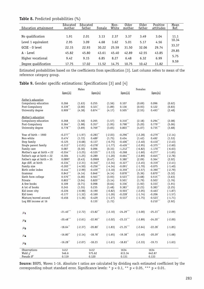
283

Estimated probabilities based on the coefficients from specification [3]. Last column refers to mean of the reference category group.

source: BHPS, Waves 1-16. Absolute t ratios are calculated by dividing each estimated coefficient by the correspondingrobuststandarderror.Significancelevels:*p<0.1,**p<0.05,***p<0.01.

table 8. Predicted probabilities (%)

table 9. Gender specific estimations: Specifications [3] and [4]

Education attainment Educated mother

Educated father Female

Non- White

Older mother

Older father

Positive attitudes

Mean Ref.

No qualification 1.91 2.01 3.13 2.37 3.37 3.49 3.04 11.1

Level 1 equivalent 2.95 3.09 4.68 3.62 5.01 5.17 4.56 10.34

GCSE - O level 22.15 22.93 30.22 25.59 31.50 32.06 29.74 33.37

A - Level 45.82 45.80 43.61 45.40 42.89 42.55 43.85 29.85

Higher vocational 9.42 9.15 6.85 8.27 6.48 6.32 6.99 5.75

Degree qualification 17.75 17.02 11.52 14.75 10.75 10.42 11.82 9.59

Spec[3] Males

Spec[4]

Spec[3] Females

Spec[4]

Father’s education Compulsory education 0.266 (1.63) 0.255 (1.56) 0.107 (0.69) 0.096 (0.62) Post-Compulsory 0.339** (2.00) 0.321* (1.89) 0.136 (0.93) 0.122 (0.83) University degree 0.909*** (4.38) 0.874*** (4.17) 0.505** (2.55) 0.493** (2.48) Mother’s education Compulsory education 0.268 (1.58) 0.265 (1.57) 0.310** (2.18) 0.294** (2.08) Post-Compulsory 0.364** (1.98) 0.357* (1.95) 0.798*** (5.20) 0.779*** (5.06) University degree 0.778*** (3.69) 0.769*** (3.65) 0.803*** (4.07) 0.735*** (3.68) Year of birth – 1900 -0.277** (-1.97) -0.283** (-2.03) -0.296** (-2.28) -0.279** (-2.14) Non-white 0.474* (1.72) 0.489* (1.75) 0.454 (1.42) 0.492 (1.53) Step family -0.125 (-0.68) -0.137 (-0.75) -0.406** (-2.40) -0.410** (-2.43) Single parent family -0.313** (-2.01) -0.278* (-1.77) -0.426*** (-2.95) -0.375*** (-2.60) Family care 0.087 (0.30) 0.096 (0.33) -1.212*** (-6.82) -1.170*** (-6.63) Mother's age at birth < 22 -0.554*** (-3.25) -0.535*** (-3.13) -0.268 (-1.60) -0.277* (-1.65) Father's age at birth < 22 -0.304 (-1.25) -0.289 (-1.20) -0.664*** (-2.89) -0.645*** (-2.78) Father's age at birth > 35 0.0897 (0.43) 0.0969 (0.47) 0.380** (2.09) 0.364** (2.02) Age diff. at birth -0.334** (-2.31) -0.340** (-2.34) -0.327** (-2.45) -0.319** (-2.41) Family size -0.265*** (-4.50) -0.256*** (-4.34) -0.091* (-1.70) -0.075 (-1.40) Birth order index -0.444*** (-2.99) -0.459*** (-3.10) -0.359** (-2.57) -0.390*** (-2.79) Grammar 0.843*** (4.14) 0.846*** (4.14) 0.878*** (5.36) 0.870*** (5.32) Sixth form college 0.570*** (4.00) 0.563*** (3.93) 0.523*** (3.68) 0.515*** (3.63) Private 0.803*** (3.04) 0.820*** (3.14) 0.501* (1.79) 0.503* (1.76) A few books 0.109 (0.71) 0.098 (0.64) 0.336* (1.92) 0.333* (1.91) A lot of books 0.245 (1.55) 0.235 (1.48) 0.383** (2.23) 0.383** (2.25) Kid inner city -0.226 (-0.98) -0.190 (-0.82) -0.503** (-2.05) -0.463* (-1.87) Kid town -0.177 (-1.32) -0.169 (-1.26) -0.228* (-1.74) -0.206 (-1.57) Mixture/moved around -0.456 (-1.36) -0.429 (-1.27) -0.537* (-1.75) -0.523* (-1.71) Log HH income at 16 0.135* (1.72) 0.210*** (2.92)

-21.40*** (-2.72) -23.82** (-2.10) -24.29*** (-3.00) -25.23** (-2.09)

-20.48*** (-2.61) -22.90** (-2.02) -23.33*** (-2.89) -24.20** (-2.00)

-18.64** (-2.37) -20.80* (-1.83) -21.35*** (-2.64) -22.28* (-1.85)

-16.80** (-2.14) -18.78* (-1.65) -19.38** (-2.40) -20.29* (-1.68)

-16.28** (-2.07) -18.23 (-1.61) -18.83** (-2.33) -19.73 (-1.63) Observations 1412 1412 1634 1634 Wald χ2 546.6 575.62 613.34 642.87 Pseudo R2 0.119 0.120 0.131 0.133

284

Education attainment Father

Compulsory Father Post

Father Degree

Mother Compulsory

Mother Post

Mother Degree

GCSE - O level -3.96 -4.99 -13.06 -4.09 -5.56 -12.02

A - Level 2.87 3.58 6.40 3.07 3.88 5.95

Degree qualification 2.21 2.80 9.33 2.24 3.16 8.04

Education attainment Father

Compulsory Father Post

Father Degree

Mother Compulsory

Mother Post

Mother Degree

Mean Ref.

GCSE - O level 30.67 30.02 21.84 31.02 29.42 22.99 30.24

A - Level 43.22 43.60 46.03 43.00 43.92 45.97

33.85

Degree qualification 10.71 11.11 17.42 10.50 11.48 16.35

13.59

Education attainment Father

Compulsory Father Post

Father Degree

Mother Compulsory

Mother Post

Mother Degree

GCSE – O level -1.63 -2.09 -8.30 -5.01 -12.95 -12.09

A – Level 0.87 1.12 3.23 2.58 5.02 3.42

Degree qualification 0.93 1.20 5.47 2.93 8.66 8.87

Education attainment Father

Compulsory Father Post

Father Degree

Mother Compulsory

Mother Post

Mother Degree

Mean Ref.

GCSE - O level 30.50 30.27 24.50 28.44 22.28 20.92 29.68

A - Level 44.43 44.54 46.39 45.34 46.54 48.45 35.06

Degree qualification 11.46 11.60 15.64 12.75 17.59 18.92 16.09

Estimated marginal effects based on coefficients from specification [4]. They are calculated relative to indi-viduals whose father and mother have no education qualifications. The rest of the independent variables are set to the mean of the sample.

Estimated probabilities based on the coefficients from specification [4]. Last column refers to mean of the reference category group.

Estimated marginal effects based on coefficients from specification [4]. They are calculated relative to indi-viduals whose father and mother have no education qualifications. The rest of the independent variables are set to the mean of the sample.

Estimated probabilities based on the coefficients from specification [4]. Last column refers to mean of the reference category group.

table 10. Marginal effects of parental education on staying-on beyond compulsory education (%): Males

table 11. Predicted probabilities of parental education on staying-on beyond compulsory education (%): Males

table 12. Marginal effects of parental education on staying-on beyond compulsory education (%): Females

table 13. Predicted probabilities of parental education on staying-on beyond compulsory education (%): Females

285

source: BHPS, Waves 1-16. Absolute t ratios are calculated by dividing each estimated coefficient by the correspondingrobuststandarderror.Significancelevels:*p<0.1,**p<0.05,***p<0.01.

table 14. Age specific estimations: Specifications [3] and [4]

A-level University degree

Spec[3]

Spec[4]

Spec[3]

Spec[4]

Father’s education Compulsory education 0.160 (1.27) 0.156 (1.23) 0.058 (0.40) 0.054 (0.37) Post-Compulsory 0.208* (1.69) 0.195 (1.58) 0.087 (0.63) 0.087 (0.62) University degree 0.813*** (4.88) 0.793*** (4.74) 0.809*** (3.90) 0.787*** (3.77) Mother’s education Compulsory education 0.313*** (2.61) 0.298** (2.49) 0.310** (2.23) 0.298** (2.15) Post-Compulsory 0.648*** (4.91) 0.629*** (4.77) 0.795*** (5.05) 0.776*** (4.93) University degree 0.857*** (5.23) 0.818*** (4.99) 1.055*** (5.00) 1.027*** (4.86) Year of birth – 1900 -0.043 (-0.41) -0.029 (-0.28) 0.064 (0.50) 0.072 (0.56) Female 0.319*** (3.91) 0.328*** (4.00) 0.339*** (3.45) 0.335*** (3.41) Non-white 0.466* (1.77) 0.529** (1.97) 1.000*** (2.90) 1.052*** (2.98) Step family -0.354** (-2.45) -0.357** (-2.49) -0.511*** (-2.72) -0.493*** (-2.62) Single parent family -0.486*** (-3.84) -0.427*** (-3.36) -0.547*** (-3.55) -0.503*** (-3.25) Family care -0.844*** (-5.53) -0.797*** (-5.26) -1.011*** (-6.00) -0.963*** (-5.74) Mother's age at birth < 22 -0.407*** (-3.10) -0.401*** (-3.07) -0.320** (-2.06) -0.316** (-2.04) Father's age at birth < 22 -0.582*** (-3.27) -0.554*** (-3.11) -0.574*** (-2.79) -0.541*** (-2.62) Father's age at birth > 35 0.211 (1.31) 0.212 (1.32) 0.278 (1.46) 0.285 (1.50) Age diff. at birth -0.256** (-2.27) -0.264** (-2.35) -0.335*** (-2.58) -0.340*** (-2.63) Family size -0.182*** (-4.19) -0.169*** (-3.91) -0.185*** (-3.49) -0.175*** (-3.31) Birth order index -0.439*** (-3.82) -0.465*** (-4.04) -0.453*** (-3.26) -0.466*** (-3.35) Grammar 1.132*** (7.59) 1.129*** (7.58) 1.389*** (7.42) 1.368*** (7.27) Sixth form college 0.583*** (4.73) 0.570*** (4.58) 0.688*** (4.31) 0.663*** (4.12) Private 0.759*** (3.50) 0.770*** (3.57) 0.761*** (2.80) 0.762*** (2.82) A few books 0.132 (1.05) 0.124 (0.99) 0.114 (0.81) 0.109 (0.77) A lot of books 0.240* (1.89) 0.237* (1.88) 0.222 (1.55) 0.220 (1.56) Kid inner city -0.414** (-2.33) -0.378** (-2.12) -0.531*** (-2.74) -0.513*** (-2.65) Kid town -0.190* (-1.77) -0.177 (-1.63) -0.235* (-1.84) -0.229* (-1.79) Mobile -0.271 (-1.09) -0.249 (-1.01) -0.355 (-1.29) -0.349 (-1.27) Log HH income at 16 0.234*** (4.09) 0.173** (2.33) Observations 2326 2326 1699 1699 Wald χ2 546.6 575.62 613.34 642.87 Pseudo R2 0.119 0.120 0.131 0.133

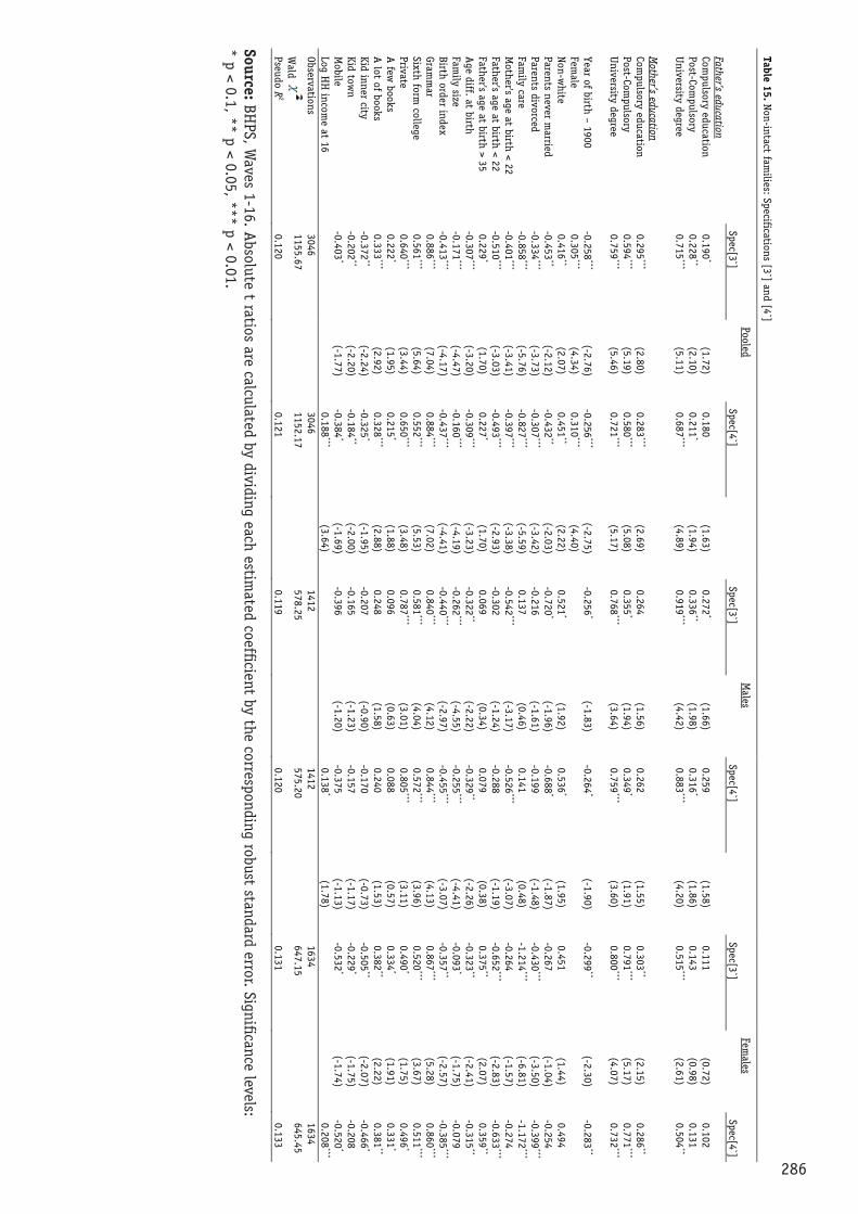
286

Table 15. Non-intact families: Specifications [3`] and [4`]

Pooled

M

ales

Females

Spec[3`]

Spec[4`]

Spec[3`]

Spec[4`]

Spec[3`]

Spec[4`]

Father’s education

Compulsory education

0.190*

(1.72) 0.180

(1.63) 0.272

* (1.66)

0.259 (1.58)

0.111 (0.72)

0.102 (0.66)

Post-Compulsory

0.228**

(2.10) 0.211

* (1.94)

0.336**

(1.98) 0.316

* (1.86)

0.143 (0.98)

0.131 (0.90)

University degree

0.715***

(5.11) 0.687

*** (4.89)

0.919***

(4.42) 0.883

*** (4.20)

0.515***

(2.61) 0.504

** (2.55)

M

other’s education

Com

pulsory education 0.295

*** (2.80)

0.283***

(2.69) 0.264

(1.56) 0.262

(1.55) 0.303

** (2.15)

0.286**

(2.03) Post-Com

pulsory 0.594

*** (5.19)

0.580***

(5.08) 0.355

* (1.94)

0.349*

(1.91) 0.791

*** (5.17)

0.771***

(5.03) U

niversity degree 0.759

*** (5.46)

0.721***

(5.17) 0.768

*** (3.64)

0.759***

(3.60) 0.800

*** (4.07)

0.732***

(3.68)

Year of birth – 1900 -0.258

*** (-2.76)

-0.256***

(-2.75) -0.256

* (-1.83)

-0.264*

(-1.90) -0.299

** (-2.30)

-0.283**

(-2.17) Fem

ale 0.305

*** (4.34)

0.310***

(4.40)

Non-w

hite 0.416

** (2.07)

0.451**

(2.22) 0.521

* (1.92)

0.536*

(1.95) 0.451

(1.44) 0.494

(1.56) Parents never m

arried -0.453

** (-2.12)

-0.432**

(-2.03) -0.720

* (-1.96)

-0.688*

(-1.87) -0.267

(-1.04) -0.254

(-1.00) Parents divorced

-0.334***

(-3.73) -0.307

*** (-3.42)

-0.216 (-1.61)

-0.199 (-1.48)

-0.430***

(-3.50) -0.399

*** (-3.23)

Family care

-0.858***

(-5.76) -0.827

*** (-5.59)

0.137 (0.46)

0.141 (0.48)

-1.214***

(-6.81) -1.172

*** (-6.61)

Mother's age at birth < 22

-0.401***

(-3.41) -0.397

*** (-3.38)

-0.542***

(-3.17) -0.526

*** (-3.07)

-0.264 (-1.57)

-0.274 (-1.63)

Father's age at birth < 22 -0.510

*** (-3.03)

-0.493***

(-2.93) -0.302

(-1.24) -0.288

(-1.19) -0.652

*** (-2.83)

-0.633***

(-2.71) Father's age at birth > 35

0.229*

(1.70) 0.227

* (1.70)

0.069 (0.34)

0.079 (0.38)

0.375**

(2.07) 0.359

** (1.99)

Age diff. at birth

-0.307***

(-3.20) -0.309

*** (-3.23)

-0.322**

(-2.22) -0.329

** (-2.26)

-0.323**

(-2.41) -0.315

** (-2.37)

Family size

-0.171***

(-4.47) -0.160

*** (-4.19)

-0.262***

(-4.55) -0.255

*** (-4.41)

-0.093*

(-1.75) -0.079

(-1.46) Birth order index

-0.413***

(-4.17) -0.437

*** (-4.41)

-0.440***

(-2.97) -0.455

*** (-3.07)

-0.357**

(-2.57) -0.385

*** (-2.78)

Gramm

ar 0.886

*** (7.04)

0.884***

(7.02) 0.840

*** (4.12)

0.844***

(4.13) 0.867

*** (5.28)

0.860***

(5.25) Sixth form

college 0.561

*** (5.64)

0.552***

(5.53) 0.581

*** (4.04)

0.572***

(3.96) 0.520

*** (3.67)

0.511***

(3.62) Private

0.640***

(3.44) 0.650

*** (3.48)

0.787***

(3.01) 0.805

*** (3.11)

0.490*

(1.75) 0.496

* (1.74)

A few

books 0.222

* (1.95)

0.215*

(1.88) 0.096

(0.63) 0.088

(0.57) 0.334

* (1.91)

0.331*

(1.90) A

lot of books 0.333

*** (2.92)

0.328***

(2.88) 0.248

(1.58) 0.240

(1.53) 0.382

** (2.22)

0.381**

(2.23) Kid inner city

-0.372**

(-2.24) -0.325

* (-1.95)

-0.207 (-0.90)

-0.170 (-0.73)

-0.505**

(-2.07) -0.466

* (-1.89)

Kid town

-0.202**

(-2.20) -0.184

** (-2.00)

-0.165 (-1.23)

-0.157 (-1.17)

-0.229*

(-1.75) -0.208

(-1.58) M

obile -0.403

* (-1.77)

-0.384*

(-1.69) -0.396

(-1.20) -0.375

(-1.13) -0.532

* (-1.74)

-0.520*

(-1.71) Log H

H incom

e at 16

0.188

*** (3.64)

0.138*

(1.78)

0.208

*** (2.89)

Observations 3046

3046

1412

1412

1634

1634

Wald

1155.67

1152.17

578.25

575.20

647.15

645.45

Pseudo R2

0.120

0.121

0.119

0.120

0.131

0.133

source: BHPS, W

aves 1-16. Absolute t ratios are calculated by dividing each estim

ated coefficient by the corresponding robust standard error. Significance levels:*p<0.1,**p<0.05,***p<0.01.

287

referencesAmato, P.R. and B. Keith (1991): “Parental Divorce and the Well Being of Children: A Meta-Analysis”. Psychological Bulletin, 110:26-47.

Amato, P.R. (2001): “Children of Divorce in the 1990s: an Update of the Amato and Keith (1991) Meta-analysis”. Journal of Family Psychology, 153:355-70.

Bauer, P. and Riphahn, R. (2006): “Timing of School Tracking as a Determinant of Intergenerational Transmission of Education”. Economic Letters, 91:90-97.

Bauer, P. and Riphahn, R. (2006): “Education and its Intergenerational Transmission: Country an Origin-Specific Evidence for Natives and Immigrants from Switzerland”. Portuguese Economic Journal, 5(2):89-110.

Black, S., P. Devereux and G. Kjell (2005): “Why the Apple Doesn’t Fall Far: Understanding Intergenerational Transmission of Human Capital”. American Economic Review, 95(1):437-449.

Black, S., P. Devereux and G. Kjell (2009): “Like father, like son? A note on the intergenerational transmission of IQ scores”. Economics Letters, Elsevier, 105(1):138-140.

Blanden, J., P. Gregg and S. Machin (2003): “Changes in Educational Inequality”, CMPO working paper series number 03/079.

Blanden, J. and P. Gregg (2004): “Family Income and Educational Attainments: A Review of Approaches and Evidence for Britain”. Oxford University Press, 20(2):245-263.

Blanden, J. and S. Machin (2004): “Educational Inequality and the Expansion of UK Higher Education”. Scottish Journal of Political Economy, 51(2):230-249.

Blanden, J., P. Gregg and S. Machin (2005): “Intergenerational Mobility in Europe and North America”, A Report Supported by Sutton Trust, Centre for Economic Performance, London, mimeo.

Blanden, J., P. Gregg and L. Macmillan (2007): “Accounting for Intergenerational Income Persistence: Noncognitive Skills, Ability and Education”. The Economic Journal, 117, C43-C60.

Blanden, J. and S. Machin (2007): “Recent Changes in Intergenerational Mobility in Britain”. Report for Sutton Trust.

Behrman, J. and M. Rosenzweig (2002): “Does Increasing Women’s Schooling Raise the Schooling of the Next Generation?”. American Economic Review, 92(1):323-334.

Behrman, J. and M. Rosenzweig (2005): “Does Increasing Women’s Schooling Raise the Schooling of the Next Generation? Replay”. American Economic Review, 95(5):1745-1751.

Böheim, R. and J. Ermisch (2001): “Partnership Dissolution in the UK – the Role of Economic

288

Circumstances”. Oxford Bulletin of Economics and Statistics, 63:197-208.

Booth, A. and H. Kee (2009): “Birth Order Matters: The Effect of Family Size and Birth Order on Educational Attainment”. Journal of Population Economics, Springer, 22(2):367-397.

Boudon, R., (1973): “L’inégalité des Chances”, A. Colin, Paris.

Brunnello, G. and D. Checchi (2007): “Does School Tracking Affect Equality of Opportunity? New International Evidence”. Economic Policy, CEPR, 22:781-861.

Chechhi, D., (2006): “The Economics of Education: Human Capital, Family Background and Inequality”. Cambridge University Press.

Cameron, S. and J. Heckman (1998): “Life Cycle Schooling and Dynamic Selection Bias: Models and Evidence for Five Cohorts of American Males”. Journal of Political Economy, 106: 262-333.

Cameron, S. and J. Heckman (2001): “”The Dynamics of Educational Attainment for Black, Hispanic and White Males”. Journal of Political Economy, 109(3):455-499.

Cameron, S. and C. Taber (2004). “Estimation of Educational Borrowing Constraint Using Returns to Schooling”. Journal of Public Economics, 112(1).

Cameron, C. and P. Trivedi (2005): “Microeconometrics: Methods and Applications”, Cambridge University Press.

Carneiro, P. and J. Heckman, J. (2002). “The Evidence of Credit Constraints in Post-Secondary Schooling”. Economic Journal, 112(482):705-734.

Carneiro, P. and J. Heckman (2003). “Human Capital Policy”. Inequality in America: What Role for Human Capital Policy?”. MIT press, Cambridge, MA.

Carneiro, P., K. Hansen, and J. Heckman (2003): “Estimating Distribution of Treatment Effect with an Application to the Return to Schooling and Measurement Effect of Uncertainty on College Choice”. International Economic Review, 2(44).

Challen, A., S. Machin and S. McNally (2008): “Schools in England: Structures, Teachers and Evaluation”. Programma Education, FGA working paper, number 1.

Chevalier, A., C. Harmon, V. O’Sullivan and L. Walker (2005): “The Impact of Parental Income and Education on the Schooling of Their Children”. IZA Discussion Papers 1496, Institute for the Study of Labor (IZA).

Chevalier, A., D. Kenny and M. Dorren (2003). “A Multi-Country Study of Inter-generational Education Mobility”. ISSC Discussion Paper 2003/06, Dublin.

Chevalier, A. and G. Lanot (2002): “The Relative Effect of Family Characteristics and Financial

289

Situation on Educational Achievement”. Education Economics, 10(2).

Currie, J. and E. Moretti (2003): “Mother’s education and the intergenerational transmission of human capital: evidence from college openings”. Quarterly Journal of Economics, 118:1495–1532.

Cunha, F. and J. Heckman (2007): “The Technology of Skill Formation”, IZA Discussion Papers 56, 209-230.

Dearden, L., C. Emmerson, C. Frayne and C. Meghir (2006), “Education Subsidies and School Drop-Our Rates” CEE Discussion Papers 0053, Centre for the Economics of Education, LSE.

Dustmann, C. (2004): “Parental Background, Secondary School Track Choice and Wages”. Oxford Economic Papers 56, 209-230.

Eckstein, Z. and K. Wolpin (1999): “Why Youth Drop out of High School: The Impact of Preferences, Opportunities and Abilities”. Econometrica, 67:1295-1339.

Ermisch, J. and M. Francesconi (2001): “Family Matters: Impact of Family Background on Educational Attainments”. Economica, 68(2):137-156.

Galindo-Rueda, F. and A. Vignoles (2005): “The Declining Relative Importance of Ability in Predicting Educational Attainment”. Journal of Human Resources, 40(2):335-353.

Haveman, R. and B. Wolfe (1995): “The Determinants of Children’s Attainments: A Review of Methods and Findings”. Journal of Economic Literature, 33:1829-78.

Heineck, G. and R. Riphnahn (2007): “Intergenerational Transmission of Educational Attainment in Germany: The Last Five Decades”. IZA Discussion Paper , Nº 2985.

Keane, M. and K. Wolpin (2001): “The Effect of Parental Transfers and Borrowing Constraints on Educational Attainment”. International Economic Review, 42:1051-1103.

Lauer, C., (2002): “A Model of Education Attainment: Application to the German Case”. ZEW Discussion Paper, Nº 02-06.

Lauer, C., (2003): “Family background, cohort and education: a French-German comparison based on a multivariate ordered probit model of educational attainment”. Labour Economics, 10:231-251.

Machin, S., (2008): “The new economics of education: methods, evidence and policy”. Journal of Population Economics, 21:1-19.

Machin, S. And A. Vignoles (2006): “Educational Policy in the UK”, Centre for Economics of Education, Discussion paper number CEEDP0057.

290

Machin, S. And A. Vignoles (2004): “Education Inequality: The Widening Socio-Economic Gap”. Fiscal Studies, 25(2):107-128.

Mare, R., (1980): “Social Background and School Continuation Decisions”. Journal of the American Statistical Association, 75:295-305.

McNally, S., (2005): “Reforms to schooling in the UK:A Review of Some Major Reforms and their Evaluation”. German Economic Review, 6(3): 287-296.

Oreopoulos, P., (2006): “The Compelling Effects of Compulsory Schooling: Evidence from Canada”. Canadian Journal of Economics, 39(1):22-52.

Piketty, T., (2007): “Theories of Persistent Inequality and Intergenerational Mobility”, Atkinson, A.B. and Bourguignon, F. (eds.). Handbook of Income Distribution, vol. 1, Elsevier Science, North Holland, 429-476.

Plug, E., (2004): “Estimating the Effect of Mother’s Schooling on Children’s Schooling Using a Sample of Adoptees”. American Economic Review, 94(1):358-368.

Plug, E. and W. Vijverberg (2003): “Schooling, Family Background and Adoption: Is it Nature or Nurture?”. Journal of Political Economy, 111(3):611-641.

Plug, E. and W. Vijverberg (2005): “Does Family Income Matter for Schooling Outcomes? Using Adoptees as a Natural Experiment”. Economic Journal, 115(506):879-906.

Riphahn, R., (2003): “Cohort Effects in the Educational Attainment of Second Generation Immigrants in Germany: An Analysis of Census Data”. Journal of Population Economics, 16(4):711-737.

Sacerdote, B., (2002): “The Nature and the Nurture of Economic Outcomes”. American Economic Review, Papers and Proceedings, 92: 344-348.

Todd, P. and K. Wolpin (2006): “Assessing the Impact of a School Subsidy Program in Mexico”. American Economic Review, 96(5):1384-1417.

Sacerdote, B., (2002): “The Nature and the Nurture of Economic Outcomes”, American Economic Review, Papers and Proceedings, 92: 344-348.

Walker, I. and Y. Zhu (2008). “The College Wage Premium and the Expansion of Higher Education in the UK”. The Scandinavian Journal of Economics, 110(4): 695–709.

Walker, I. and Y. Zhu (2008): “Child Support and Educational Outcomes: Evidence from the British Household Panel Survey”. Studies in Economics 0811, Department of Economics, University of Kent.