chapter · chapter 4 finite elemen t appro ximation 4.1 in tro duction our goal in this c hapter is...

Chapter 4

Finite Element Approximation

4.1 Introduction

Our goal in this chapter is the development of piecewise-polynomial approximations U

of a two- or three-dimensional function u. For this purpose, it su�ces to regard u as

being known and to determine U as its interpolant on a domain . Concentrating on

two dimensions for the moment, let us partition into a collection of �nite elements and

write U in the customary form

U(x; y) =NXj=1

cj�j(x; y): (4.1.1)

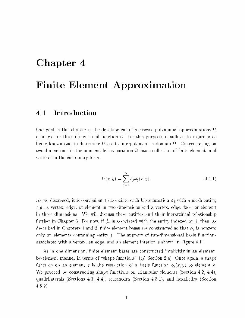
As we discussed, it is convenient to associate each basis function �j with a mesh entity,

e.g., a vertex, edge, or element in two dimensions and a vertex, edge, face, or element

in three dimensions. We will discuss these entities and their hierarchical relationship

further in Chapter 5. For now, if �j is associated with the entity indexed by j, then, as

described in Chapters 1 and 2, �nite element bases are constructed so that �j is nonzero

only on elements containing entity j. The support of two-dimensional basis functions

associated with a vertex, an edge, and an element interior is shown in Figure 4.1.1.

As in one dimension, �nite element bases are constructed implicitly in an element-

by-element manner in terms of \shape functions" (cf. Section 2.4). Once again, a shape

function on an element e is the restriction of a basis function �j(x; y) to element e.

We proceed by constructing shape functions on triangular elements (Section 4.2, 4.4),

quadrilaterals (Sections 4.3, 4.4), tetrahedra (Section 4.5.1), and hexahedra (Section

4.5.2).

1

2 Finite Element Approximation

��

��

��

��

��

��

��

��

Figure 4.1.1: Support of basis functions associated with a vertex, edge, and elementinterior (left to right).

4.2 Lagrange Shape Functions on Triangles

Perhaps the simplest two-dimensional Lagrangian �nite element basis is a piecewise-linear

polynomial on a grid of triangular elements. It is the two-dimensional analog of the hat

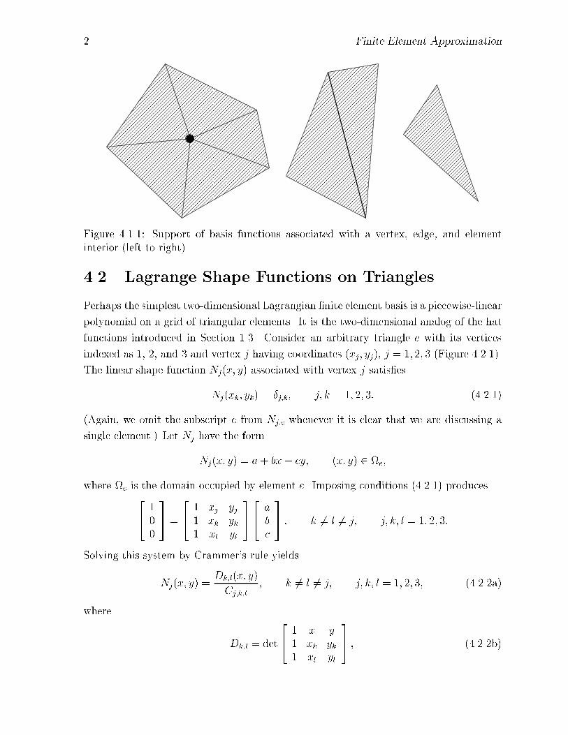
functions introduced in Section 1.3. Consider an arbitrary triangle e with its vertices

indexed as 1, 2, and 3 and vertex j having coordinates (xj; yj), j = 1; 2; 3 (Figure 4.2.1).

The linear shape function Nj(x; y) associated with vertex j satis�es

Nj(xk; yk) = �j;k; j; k = 1; 2; 3: (4.2.1)

(Again, we omit the subscript e from Nj;e whenever it is clear that we are discussing a

single element.) Let Nj have the form

Nj(x; y) = a+ bx + cy; (x; y) 2 e;

where e is the domain occupied by element e. Imposing conditions (4.2.1) produces24 1

00

35 =

24 1 xj yj

1 xk yk1 xl yl

3524 a

bc

35 ; k 6= l 6= j; j; k; l = 1; 2; 3:

Solving this system by Crammer's rule yields

Nj(x; y) =Dk;l(x; y)

Cj;k;l; k 6= l 6= j; j; k; l = 1; 2; 3; (4.2.2a)

where

Dk;l = det

24 1 x y1 xk yk1 xl yl

35 ; (4.2.2b)

4.2. Lagrange Shape Functions on Triangles 3

��

��

��

2

3

1

(x ,y )

(x ,y )

(x ,y )1 1

2 2

3 3

Figure 4.2.1: Triangular element with vertices 1; 2; 3 having coordinates (x1; y1), (x2; y2),and (x3; y3).

2

1

3

N

1

2

3

φ1

1

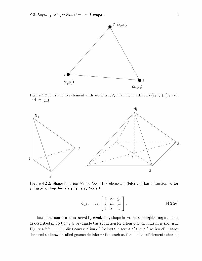
Figure 4.2.2: Shape function N1 for Node 1 of element e (left) and basis function �1 fora cluster of four �nite elements at Node 1.

Cj;k;l = det

24 1 xj yj

1 xk yk1 xl yl

35 : (4.2.2c)

Basis functions are constructed by combining shape functions on neighboring elements

as described in Section 2.4. A sample basis function for a four-element cluster is shown in

Figure 4.2.2. The implicit construction of the basis in terms of shape function eliminates

the need to know detailed geometric information such as the number of elements sharing


a node. Placing the three nodes at element vertices guarantees a continuous basis. While

interpolation at three non-colinear points is (necessary and) su�cient to determine a

unique linear polynomial, it will not determine a continuous approximation. With vertex

placement, the shape function (e.g., Nj) along any element edge is a linear function of

a variable along that edge. This linear function is determined by the nodal values at

the two vertex nodes on that edge (e.g., j and k). As shown in Figure 4.2.2, the shape

function on a neighboring edge is determined by the same two nodal values; thus, the

basis (e.g., �j) is continuous.

The restriction of U(x; y) to element e has the form

U(x; y) = c1N1(x; y) + c2N2(x; y) + c3N3(x; y); (x; y) 2 e: (4.2.3)

Using (4.2.1), we have cj = U(xj ; yj), j = 1; 2; 3.

The construction of higher-order Lagrangian shape functions proceeds in the same

manner. In order to construct a p th-degree polynomial approximation on element e, we

introduce Nj(x; y), j = 1; 2; : : : ; np, shape functions at np nodes, where

np =(p+ 1)(p+ 2)

2(4.2.4)

is the number of monomial terms in a complete polynomial of degree p in two dimensions.

We may write a shape function in the form

Nj(x; y) =

npXi=1

aiqi(x; y) = aTq(x; y) (4.2.5a)

where

qT (x; y) = [1; x; y; x2; xy; y2; : : : ; yp]: (4.2.5b)

Thus, for example, a second degree (p = 2) polynomial would have n2 = 6 coe�cients

and

qT (x; y) = [1; x; y; x2; xy; y2]:

Including all np monomial terms in the polynomial approximation ensures isotropy in the

sense that the degree of the trial function is conserved under coordinate translation and

rotation.

With six parameters, we consider constructing a quadratic Lagrange polynomial by

placing nodes at the vertices and midsides of a triangular element. The introduction of

nodes is unnecessary, but it is a convenience. Indexing of nodes and other entities will be

discussed in Chapter 5. Here, since we're dealing with a single element, we number the


��

��

��

��

��

��

��

��

��

��

��

��

��

��

��

��

��

��

��

1

2

3

4

56

1

2

3

4 5

6

78

9 10

Figure 4.2.3: Arrangement of nodes for quadratic (left) and cubic (right) Lagrange �niteelement approximations.

nodes from 1 to 6 as shown in Figure 4.2.3. The shape functions have the form (4.2.5)

with n2 = 6

Nj = a1 + a2x + a3y + a4x2 + a5xy + a6y

2;

and the six coe�cients aj, j = 1; 2; : : : ; 6, are determined by requiring

Nj(xk; yk) = �j;k; j; k = 1; 2; : : : ; 6:

The basis

�j = [N�e=1Nj;e(x; y)

is continuous by virtue of the placement of the nodes. The shape function Nj;e is a

quadratic function of a local coordinate on each edge of the triangle. This quadratic

function of a single variable is uniquely determined by the values of the shape functions

at the three nodes on the given edge. Shape functions on shared edges of neighboring

triangles are determined by the same nodal values; hence, ensuring that the basis is

globally of class C0.

The construction of cubic approximations would proceed in the same manner. A

complete cubic in two dimensions has 10 parameters. These parameters can be deter-

mined by selecting 10 nodes on each element. Following the reasoning described above,

we should place four nodes on each edge since a cubic function of one variable is uniquely

determined by prescribing four quantities. This accounts for nine of the ten nodes. The

last node can be placed at the centroid as shown in Figure 4.2.3.

The construction of Lagrangian approximations is straight forward but algebraically

complicated. Complexity can be signi�cantly reduced by using one of the following two

coordinate transformations.


��

��

��

��

��

��

��

��

3 (x ,y )

1 (x ,y )

y

x

1 1

3 3

1 (0,0) 2 (1,0)

3 (0,1)

ξ

η

N = 0

21

13

13

N = 1

2 (x ,y )2 2

N = 0

21N = 1

Figure 4.2.4: Mapping an arbitrary triangular element in the (x; y)-plane (left) to acanonical 45� right triangle in the (�; �)-plane (right).

1. Transformation to a canonical element. The idea is to transform an arbitrary

element in the physical (x; y)-plane to one having a simpler geometry in a computational

(�; �)-plane. For purposes of illustration, consider an arbitrary triangle having vertex

nodes numbered 1, 2, and 3 which is mapped by a linear transformation to a unit 45�

right triangle, as shown in Figure 4.2.4.

Consider N12 and N1

3 as de�ned by (4.2.2). (A superscript 1 has been added to

emphasize that the shape functions are linear polynomials.) The equation of the line

connecting Nodes 1 and 3 of the triangular element shown on the left of Figure 4.2.4 is

N12 = 0. Likewise, the equation of a line passing through Node 2 and parallel to the

line passing through Nodes 1 and 3 is N12 = 1. Thus, to map the line N1

2 = 0 onto the

line � = 0 in the canonical plane, we should set � = N12 (x; y). Similarly, the line joining

Nodes 1 and 2 satis�es the equation N13 = 0. We would like this line to become the line

� = 0 in the transformed plane, so our mapping must be � = N13 (x; y). Therefore, using

(4.2.2)

� = N12 (x; y) =

det

24 1 x y

1 x1 y11 x3 y3

35

det

24 1 x2 y2

1 x1 y11 x3 y3

35; � = N1

3 (x; y) =

det

24 1 x y

1 x1 y11 x2 y2

35

det

24 1 x3 y3

1 x1 y11 x2 y2

35: (4.2.6)

As a check, evaluate the determinants and verify that (x1; y1)! (0; 0), (x2; y2)! (1; 0),

and (x3; y3)! (0; 1).

Polynomials may now be developed on the canonical triangle to simplify the algebraic


��

��

��

��

��

��

��

��

��

��

��

��

��

��

��

��

��

��

��

��

2

3

4

5

6

7

8

1

9

N = 0

N = 0

N = 1/3N = 2/310

11

11

11

12

Figure 4.2.5: Geometry of a triangular �nite element for a cubic polynomial Lagrangeapproximation.

complexity and subsequently transformed back to the physical element.

2. Transformation using triangular coordinates. A simple procedure for constructing

Lagrangian approximations involves the use of a redundant coordinate system. The

construction may be described in general terms, but an example su�ces to illustrate the

procedure. Thus, consider the construction of a cubic approximation on the triangular

element shown in Figure 4.2.5. The vertex nodes are numbered 1, 2, and 3; edge nodes

are numbered 4 to 9; and the centroid is numbered as Node 10.

Observe that

� the line N11 = 0 passes through Nodes 2, 6, 7, and 3;

� the line N11 = 1=3 passes through Nodes 5, 10, and 8; and

� the line N11 = 2=3 passes through Nodes 4 and 9.

Since N31 must vanish at Nodes 2 - 10 and be a cubic polynomial, it must have the form

N31 (x; y) = �N1

1 (N11 � 1=3)(N1

1 � 2=3)

where the constant � is determined by normalizing N31 (x1; y1) = 1. Since N1

1 (x1; y1) = 1,

we �nd � = 9=2 and

N31 (x; y) =

9

2N1

1 (N11 � 1=3)(N1

1 � 2=3):

The shape function for an edge node is constructed in a similar manner. For example,

in order to obtain N34 we observe that

� the line N12 = 0 passes through Nodes 1, 9, 8, and 3;


� the line N11 = 0 passes through Nodes 2, 6, 7, and 3; and

� the line N11 = 1=3 passes through Nodes 5, 10, and 8.

Thus, N34 must have the form

N34 (x; y) = �N1

1N12 (N

11 � 1=3):

Normalizing N34 (x4; y4) = 1 gives

N34 (x4; y4) = �

2

3

1

3(2

3� 1

3):

Hence, � = 27=2 and

N34 (x; y) =

27

2N11N

12 (N

11 � 1=3):

Finally, the shape function N310 must vanish on the boundary of the triangle and is,

thus, determined as

N310(x; y) = 27N1

1N12N

13 :

The cubic shape functions N31 , N

34 , and N3

10 are shown in Figure 4.2.6.

The three linear shape functions N1j , j = 1; 2; 3, can be regarded as a redundant

coordinate system known as \triangular" or \barycentric" coordinates. To be more

speci�c, consider an arbitrary triangle with vertices numbered 1, 2, and 3 as shown

in Figure 4.2.7. Let

�1 = N11 ; �2 = N1

2 ; �3 = N13 ; (4.2.7)

and de�ne the transformation from triangular to physical coordinates as

24 x

y1

35 =

24 x1 x2 x3

y1 y2 y31 1 1

3524 �1�2�3

35 : (4.2.8)

Observe that (�1; �2; �3) has value (1,0,0) at vertex 1, (0,1,0) at vertex 2 and (0,0,1) at

vertex 3.

An alternate, and more common, de�nition of the triangular coordinate system in-

volves ratios of areas of subtriangles to the whole triangle. Thus, let P be an arbitrary

point in the interior of the triangle, then the triangular coordinates of P are

�1 =AP23

A123; �2 =

AP31

A123; �3 =

AP12

A123; (4.2.9)

where A123 is the area of the triangle, AP23 is the area of the subtriangle having vertices

P , 2, 3, etc.


0

0.2

0.4

0.6

0.8

1 0

0.2

0.4

0.6

0.8

1−0.2

0

0.2

0.4

0.6

0.8

1

1.2

0

0.2

0.4

0.6

0.8

1 0

0.2

0.4

0.6

0.8

1−0.4

−0.2

0

0.2

0.4

0.6

0.8

1

1.2

0

0.2

0.4

0.6

0.8

1 0

0.2

0.4

0.6

0.8

10

0.2

0.4

0.6

0.8

1

Figure 4.2.6: Cubic Lagrange shape functions associated with a vertex (left), anedge(right), and the centroid (bottom) of a right 45� triangular element.

The triangular coordinate system is redundant since two quantities su�ce to locate

a point in a plane. This redundancy is expressed by the third of equations (4.2.8), which

states that

�1 + �2 + �3 = 1:

This relation also follows by adding equations (4.2.9).

Although seemingly distinct, triangular coordinates and the canonical coordinates are

closely related. The triangular coordinate �2 is equivalent to the canonical coordinate �

and �3 is equivalent to �, as seen from (4.2.6) and (4.2.7).

Problems

1. With reference to the nodal placement and numbering shown on the left of Figure

4.2.3, construct the shape functions for Nodes 1 and 4 of the quadratic Lagrange

polynomial. Derive your answer using triangular coordinates. Having done this,

also express your answer in terms of the canonical (�; �) coordinates. Plot or sketch


3 (0,0,1)

2 (0,1,0)

1 (1,0,0) P( ζ ,ζ ,ζ )1 2 3

ζ = 0

ζ = 0

ζ = 0

1

2

3

1ζ = 1

Figure 4.2.7: Triangular coordinate system.

the two shape functions on the canonical element.

2. A Lagrangian approximation of degree p on a triangle has three nodes at the vertices

and p � 1 nodes along each edge that are not at vertices. As we've discussed,

the latter placement ensures continuity on a mesh of triangular elements. If no

additional nodes are placed on edges, how many nodes are interior to the element

if the approximation is to be complete?

4.3 Lagrange Shape Functions on Rectangles

The triangle in two dimensions and the tetrahedron in three dimensions are the poly-

hedral shapes having the minimum number of edges and faces. They are optimal for

de�ning complete C0 Lagrangian polynomials. Even so, Lagrangian interpolants are

simple to construct on rectangles and hexahedra by taking products of one-dimensional

Lagrange polynomials. Multi-dimensional polynomials formed in this manner are called

\tensor-product" approximations. we'll proceed by constructing polynomial shape func-

tions on canonical 2 � 2 square elements and mapping these elements to an arbitrary

quadrilateral elements. We describe a simple bilinear mapping here and postpone more

complex mappings to Chapter 5.

We consider the canonical 2� 2 square f(�; �)j � 1 � �; � � 1g shown in Figure 4.3.1.

For simplicity, the vertices of the element have been indexed with a double subscript

as (1; 1), (2; 1), (1; 2), and (2; 2). At times it will be convenient to index the vertex

coordinats as �1 = �1, �2 = 1, �1 = �1, and �2 = 1. With nodes at each vertex, we

construct a bilinear Lagrangian polynomial U(�; �) whose restriction to the canonical

4.3. Lagrange Shape Functions on Rectangles 11

��

��

��

��

��

��

��

��

��

��

��

��

��

x

1,1

1,2y 1,2

2,1

2,2 3,2 2,2

2,13,11,1

3,3 2,31,3

Figure 4.3.1: Node indexing for canonical square elements with bilinear (left) and bi-quadratic (right) polynomial shape functions.

element has the form

U(�; �) = c1;1N1;1(�; �) + c2;1N2;1(�; �) + c2;2N2;2(�; �) + c1;2N1;2(�; �): (4.3.1a)

As with Lagrangian polynomials on triangles, the shape function Ni;j(�; �) satis�es

Ni;j(�k; �l) = �i;k�j;l; k; l = 1; 2: (4.3.1b)

Once again, U(�k; �l) = ck;l; however, now Ni;j is the product of one-dimensional hat

functions

Ni;j(�; �) = �Ni(�) �Nj(�) (4.3.1c)

with

�N1(�) =1� �

2; (4.3.1d)

�N2(�) =1 + �

2; �1 � � � 1: (4.3.1e)

Similar formulas apply to �Nj(�), j = 1; 2, with � replaced by � and i replaced by j.

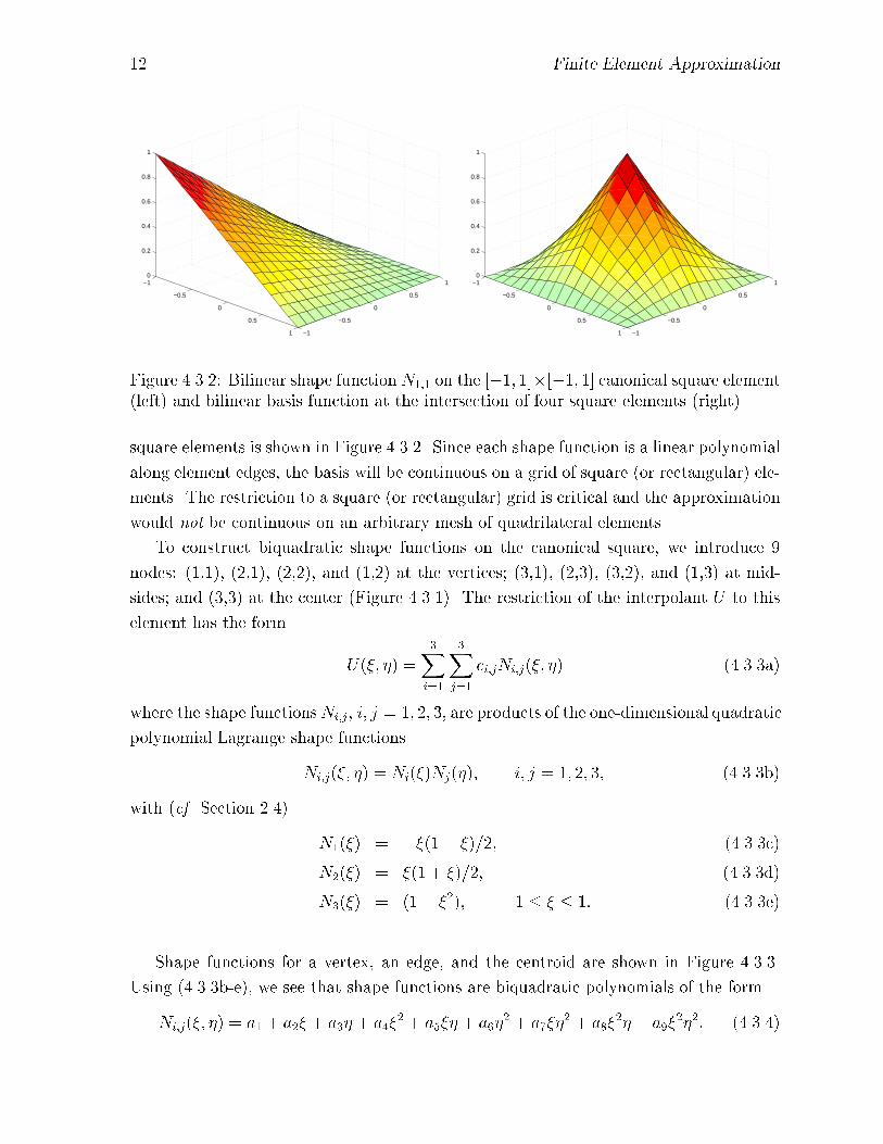
The shape function N1;1 is shown in Figure 4.3.2. By examination of either this �gure or

(4.3.1c-e), we see that Ni;j(�; �) is a bilinear function of the form

Ni;j(�; �) = a1 + a2� + a3� + a4��; �1 � �; � � 1: (4.3.2)

The shape function is linear along the two edges containing node (i; j) and it vanishes

along the two opposite edges.

A basis may be constructed by uniting shape functions on elements sharing a node.

The piecewise bilinear basis functions �i;j when Node (i; j) is at the intersection of four


−1

−0.5

0

0.5

1 −1

−0.5

0

0.5

10

0.2

0.4

0.6

0.8

1

−1

−0.5

0

0.5

1 −1

−0.5

0

0.5

10

0.2

0.4

0.6

0.8

1

Figure 4.3.2: Bilinear shape function N1;1 on the [�1; 1]�[�1; 1] canonical square element(left) and bilinear basis function at the intersection of four square elements (right).

square elements is shown in Figure 4.3.2. Since each shape function is a linear polynomial

along element edges, the basis will be continuous on a grid of square (or rectangular) ele-

ments. The restriction to a square (or rectangular) grid is critical and the approximation

would not be continuous on an arbitrary mesh of quadrilateral elements.

To construct biquadratic shape functions on the canonical square, we introduce 9

nodes: (1,1), (2,1), (2,2), and (1,2) at the vertices; (3,1), (2,3), (3,2), and (1,3) at mid-

sides; and (3,3) at the center (Figure 4.3.1). The restriction of the interpolant U to this

element has the form

U(�; �) =3X

i=1

3Xj=1

ci;jNi;j(�; �) (4.3.3a)

where the shape functionsNi;j, i; j = 1; 2; 3, are products of the one-dimensional quadratic

polynomial Lagrange shape functions

Ni;j(�; �) = �Ni(�) �Nj(�); i; j = 1; 2; 3; (4.3.3b)

with (cf. Section 2.4)

�N1(�) = ��(1� �)=2; (4.3.3c)

�N2(�) = �(1 + �)=2; (4.3.3d)

�N3(�) = (1� �2); �1 � � � 1: (4.3.3e)

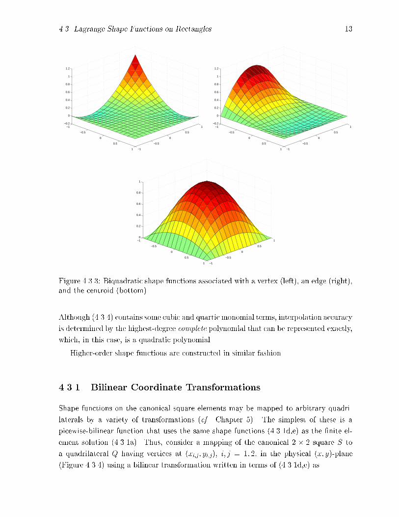
Shape functions for a vertex, an edge, and the centroid are shown in Figure 4.3.3.

Using (4.3.3b-e), we see that shape functions are biquadratic polynomials of the form

Ni;j(�; �) = a1 + a2� + a3� + a4�2 + a5�� + a6�

2 + a7��2 + a8�

2� + a9�2�2: (4.3.4)

4.3. Lagrange Shape Functions on Rectangles 13

−1

−0.5

0

0.5

1 −1

−0.5

0

0.5

1−0.2

0

0.2

0.4

0.6

0.8

1

1.2

−1

−0.5

0

0.5

1 −1

−0.5

0

0.5

1−0.2

0

0.2

0.4

0.6

0.8

1

1.2

−1

−0.5

0

0.5

1 −1

−0.5

0

0.5

10

0.2

0.4

0.6

0.8

1

Figure 4.3.3: Biquadratic shape functions associated with a vertex (left), an edge (right),and the centroid (bottom).

Although (4.3.4) contains some cubic and quartic monomial terms, interpolation accuracy

is determined by the highest-degree complete polynomial that can be represented exactly,

which, in this case, is a quadratic polynomial.

Higher-order shape functions are constructed in similar fashion.

4.3.1 Bilinear Coordinate Transformations

Shape functions on the canonical square elements may be mapped to arbitrary quadri-

laterals by a variety of transformations (cf. Chapter 5). The simplest of these is a

picewise-bilinear function that uses the same shape functions (4.3.1d,e) as the �nite el-

ement solution (4.3.1a). Thus, consider a mapping of the canonical 2 � 2 square S to

a quadrilateral Q having vertices at (xi;j; yi;j), i; j = 1; 2, in the physical (x; y)-plane

(Figure 4.3.4) using a bilinear transformation written in terms of (4.3.1d,e) as


��

��

��

��

��

��

��

��

��

��1,1 (x ,y )

(x ,y )

2,2 (x ,y )

1,2

(x ,y )

x

y

11

21

22

12

11

21

22

12η

2,1

2,21,2

1,1 2,1

1 1

ξ

1

1

Figure 4.3.4: Bilinear mapping of the canonical square to a quadrilateral.

�x(�; �)y(�; �)

�=

2Xi=1

2Xj=1

�xijyij

�Ni;j(�; �); (4.3.5)

where Ni;j(�; �) is given by (4.3.1b).

The transformation is linear on each edge of the element. In particular, transforming

the edge � = �1 to the physical edge (x11; y11 - (x21; y21) yields�xy

�=

�x11y11

�1� �

2+

�x21y21

�1 + �

2; �1 � � � 1:

As � varies from -1 to 1, x and y vary linearly from (x11; y11) to (x21; y21). The locations

of the vertices (1,2) and (2,2) have no e�ect on the transformation. This ensures that a

continuous approximation in the (�; �)-plane will remain continuous when mapped to the

(x; y)-plane. We have to ensure that the mapping is invertible and we'll show in Chapter

5 that this is the case when Q is convex.

Problems

1. As noted, interpolation errors of the biquadratic approximation (4.3.3) are the same

order as for a quadratic approximation on a triangle. Thus, for example, the L2

error in interpolating a smooth function u(x; y) by a piecewise biquadratic function

U(x; y) is O(h3), where h is the length of the longest edge of an element. The

extra degrees of freedom associated with the cubic and quartic terms do not gen-

erally improve the order of accuracy. Hence, we might try to eliminate some shape

functions and reduce the complexity of the approximation. Unknowns associated

with interior shape functions are only coupled to unknowns on the element and can

easily be eliminated by a variety of techniques. Considering the biquadratic poly-

nomial in the form (4.3.3a), we might determine c3;3 so that the coe�cient of the

4.4. Hierarchical Shape Functions 15

quartic term x2y2 vanishes. Show how this may be done for a 2� 2 square canon-

ical element. Polynomials of this type have been called serendipity by Zienkiewicz

[8]. In the next section, we shall see that they are also a part of the hierarchical

family of approximations. The parameter c3;3 is said to be \constrained" since it is

prescribed in advance and not determined as part of the Galerkin procedure. Plot

or sketch shape functions associated with a vertex and a midside.

4.4 Hierarchical Shape Functions

We have discussed the advantages of hierarchical bases relative to Lagrangian bases for

one-dimensional problems in Section 2.5. Similar advantages apply in two and three di-

mensions. We'll again use the basis of Szab�o and Babu�ska [7], but follow the construction

procedure of Shephard et al. [6] and Dey et al. [5]. Hierarchical bases of degree p may

be constructed for triangles and squares. Squares are the simpler of the two, so let us

handle them �rst.

4.4.1 Hierarchical Shape Functions on Squares

We'll construct the basis on the canonical element f(�; �)j � 1 � �; � � 1g, indexingthe vertices, edges, and interiors as described for the biquadratic approximation shown

in Figure 4.3.1. The hierarchical polynomial of order p has a basis consisting of the

following shape functions.

Vertex shape functions. The four vertex shape functions are the bilinear functions

(4.3.1c-e)

N1i;j = �Ni(�) �Nj(�); i; j = 1; 2; (4.4.1a)

where

�N1(�) =1� �

2; �N2(�) =

1 + �

2: (4.4.1b)

The shape function N11;1 is shown in the upper left portion of Figure 4.4.1.

Edge shape functions. For p � 2, there are 4(p� 1) shape functions associated with

the midside nodes (3; 1), (2; 3), (3; 2), and (1; 3):

Nk3;1(�; �) = �N1(�) �N

k(�); (4.4.2a)

Nk3;2(�; �) = �N2(�) �N

k(�); (4.4.2b)

Nk1;3(�; �) = �N1(�) �N

k(�); (4.4.2c)

Nk2;3(�; �) = �N2(�) �N

k(�); k = 2; 3; : : : ; p; (4.4.2d)


where �Nk(�), k = 2; 3; : : : ; p, are the one-dimensional hierarchical shape functions given

by (2.5.8a) as

�Nk(�) =

r2k � 1

2

Z �

�1

Pk�1(�)d�: (4.4.2e)

Edge shape functions Nk3;1 are shown for k = 2; 3; 4, in Figure 4.4.1. The edge shape

functions are the product of a linear function of the variable normal to the edge to which

they are associated and a hierarchical polynomial of degree k in a variable on this edge.

The linear function ( �Nj(�), �Nj(�), j = 1; 2) \blends" the edge function ( �Nk(�), �Nk(�))

onto the element so as to ensure continuity of the basis.

Interior shape functions. For p � 4, there are (p�2)(p�3)=2 internal shape functions

associated with the centroid, Node (3; 3). The �rst internal shape function is the \bubble

function"

N4;0;03;3 = (1� �2)(1� �2): (4.4.3a)

The remaining shape functions are products of N4;0;03;3 and the Legendre polynomials as

N5;1;03;3 = N4;0;0

3;3 P1(�); (4.4.3b)

N5;0;13;3 = N4;0;0

3;3 P1(�); (4.4.3c)

N6;2;03;3 = N4;0;0

3;3 P2(�); (4.4.3d)

N6;1;13;3 = N4;0;0

3;3 P1(�)P1(�); (4.4.3e)

N6;0;23;3 = N4;0;0

3;3 P2(�); : : : : (4.4.3f)

The superscripts k, �, and �, resectively, give the polynomial degree, the degree of P�(�),

and the degree of P�(�). The �rst six interior bubble shape functions Nk;�;�3;3 , �+� = k�4,

k = 4; 5; 6, are shown in Figure 4.4.2. These functions vanish on the element boundary

to maintain continuity.

On the canonical element, the interpolant U(�; �) is written as the usual linear com-

bination of shape functions

U(�; �) =2X

i=1

2Xj=1

c1i;jN1i;j +

pXk=2

[2X

j=1

ck3;jNk3;j +

2Xi=1

cki;3Nki;3] +

pXk=4

X�+�=k�4

ck;�;�3;3 Nk;�;�3;3 :

(4.4.4)

The notation is somewhat cumbersome but it is explicit. The �rst summation identi�es

unknowns and shape functions associated with vertices. The two center summations

identify edge unknowns and shape functions for polynomial orders 2 to p. And, the

third summation identi�es the interior unknowns and shape functions of orders 4 to p.


−1

−0.5

0

0.5

1 −1

−0.5

0

0.5

10

0.2

0.4

0.6

0.8

1

−1

−0.5

0

0.5

1

−1

−0.5

0

0.5

1−0.7

−0.6

−0.5

−0.4

−0.3

−0.2

−0.1

0

−1

−0.5

0

0.5

1

−1

−0.5

0

0.5

1−0.4

−0.3

−0.2

−0.1

0

0.1

0.2

0.3

0.4

−1

−0.5

0

0.5

1

−1

−0.5

0

0.5

1−0.2

−0.15

−0.1

−0.05

0

0.05

0.1

0.15

0.2

0.25

Figure 4.4.1: Hierarchical vertex and edge shape functions for k = 1 (upper left), k = 2(upper right), k = 3 (lower left), and k = 4 (lower right).

Summations are understood to be zero when their initial index exceeds the �nal index.

A degree p approximation has 4 + 4(p� 1)+ + (p� 2)+(p� 3)+=2 unknowns and shape

functions, where q+ = max(q; 0). This function is listed in Table 4.4.1 for p ranging from

1 to 8. For large values of p there are O(p2) internal shape functions and O(p) edge

functions.

4.4.2 Hierarchical Shape Functions on Triangles

We'll express the hierarchical shape functions for triangular elements in terms of trian-

gular coordinates, indexing the vertices as 1, 2, and 3; the edges as 4, 5, and 6; and the

centroid as 7 (Figure 4.4.3). The basis consists of the following shape functions.

Vertex Shape functions. The three vertex shape functions are the linear barycentric

coordinates (4.2.7)

N1i (�1; �2; �3) = �i; i = 1; 2; 3: (4.4.5)


−1

−0.5

0

0.5

1 −1

−0.5

0

0.5

10

0.2

0.4

0.6

0.8

1

−1

−0.5

0

0.5

1 −1

−0.5

0

0.5

1−0.4

−0.3

−0.2

−0.1

0

0.1

0.2

0.3

0.4

−1

−0.5

0

0.5

1 −1

−0.5

0

0.5

1−0.4

−0.3

−0.2

−0.1

0

0.1

0.2

0.3

0.4

−1

−0.5

0

0.5

1 −1

−0.5

0

0.5

1−0.5

−0.4

−0.3

−0.2

−0.1

0

0.1

0.2

−1

−0.5

0

0.5

1 −1

−0.5

0

0.5

1−0.2

−0.15

−0.1

−0.05

0

0.05

0.1

0.15

−1

−0.5

0

0.5

1 −1

−0.5

0

0.5

1−0.5

−0.4

−0.3

−0.2

−0.1

0

0.1

0.2

Figure 4.4.2: Hierarchical interior shape functions N4;0;03;3 , N5;1;0

3;3 (top), N5;0;13;3 , N6;2;0

3;3 (mid-

dle), and N6;1;13;3 , N6;0;2

3;3 (bottom).


p Square TriangleDimension Dimension

1 4 32 8 63 12 104 17 155 23 216 30 287 38 368 47 45

Table 4.4.1: Dimension of the hierarchical basis of order p on square and triangularelements.

��

��

��

��

��

��

��

��

��

��

��

��

��

4

57

6

ζ

ζ

1

2

ξ1 (1,0,0)

3 (0,0,1)

2 (0,1,0)

Figure 4.4.3: Node placement and coordinates for hierarchical approximations on a tri-angle.

Edge shape functions. For p � 2 there are 3(p � 1) edge shape functions which are

each nonzero on one edge (to which they are associated) and vanish on the other two.

Each shape function is selected to match the corresponding edge shape function on a

square element so that a continuous approximation may be obtained on meshes with

both triangular and quadrilateral elements. Let us construct of the shape functions Nk4 ,

k = 2; 3; : : : ; p, associated with Edge 4. They are required to vanish on Edges 5 and 6

and must have the form

Nk4 (�1; �2; �3) = �1�2 ��

k(�); k = 2; 3; : : : ; p; (4.4.6a)

where ��k(�) is a shape function to be determined and � is a coordinate on Edge 4 that

has value -1 at Node 1, 0 at Node 4, and 1 at Node 2. Since Edge 4 is �3 = 0, we have

Nk4 (�1; �2; 0) = �1�2 ��

k(�); �1 + �2 = 1:


The latter condition follows from (4.2.8) with �3 = 0. Along Edge 4, �1 ranges from 1 to

0 and �2 ranges from 0 to 1 as � ranges from -1 to 1; thus, we may select

�1 = (1� �)=2; �2 = (1 + �)=2; �3 = 0: (4.4.6b)

While � may be de�ned in other ways, this linear mapping ensures that �1 + �2 = 1 on

Edge 4. Compatibility with the edge shape function (4.4.2) requires

Nk4 (�1; �2; 0) = �Nk(�) =

(1� �)(1 + �)

4��k(�)

where �Nk(�) is the one-dimensional hierarchical shape function (4.4.2e). Thus,

��k(�) =4 �Nk(�)

1� �2: (4.4.6c)

The result can be written in terms of triangular coordinates by using (4.4.6b) to obtain

� = �2 � �1; hence,

Nk4 (�1; �2; �3) = �1�2 ��

k(�2 � �1); k = 2; 3; : : : ; p: (4.4.7a)

Shape functions along other edges follow by permuting indices, i.e.,

Nk5 (�1; �2; �3) = �2�3 ��

k(�3 � �2); (4.4.7b)

Nk6 (�1; �2; �3) = �3�1 ��

k(�1 � �3); k = 2; 3; : : : ; p: (4.4.7c)

It might appear that the shape functions ��k(�) has singularities at � = �1; however, theone-dimensional hierarchical shape functions have (1� �2) as a factor. Thus, ��k(�) is a

polynomial of degree k � 2. Using (2.5.8), the �rst four of them are

��2(�) = �p6; ��3(�) = �

p10�;

��4(�) = �r

7

8(5�2 � 1); ��5(�) = �

r9

8(7�3 � 3�): (4.4.8)

Interior shape functions. The (p� 1)(p� 2)=2 internal shape functions for p � 3 are

products of the bubble function

N3;0;07 = �1�2�3 (4.4.9a)

and Legendre polynomials. The Legendre polynomials are functions of two of the three

triangular coordinates. Following Szab�o and Babu�ska [7], we present them in terms of

�2 � �1 and �3. Thus,

N4;1;07 = N3;0;0

7 P1(�2 � �1); (4.4.9b)

N4;0;17 = N3;0;0

7 P1(2�3 � 1); (4.4.9c)

N5;2;07 = N3;0;0

7 P2(�2 � �1); (4.4.9d)

N5;1;17 = N3;0;0

7 P1(�2 � �1)P1(2�3 � 1); (4.4.9e)

N5;0;27 = N3;0;0

7 P2(2�3 � 1); : : : : (4.4.9f)

4.4. Three-Dimensional Shape Functions 21

The shift in �3 ensures that the range of the Legendre polynomials is [�1; 1].Like the edge shape functions for a square (4.4.2), the edge shape functions for a

triangle (4.4.7) are products of a function on the edge (��k(�i��j)) and a function (�i�j; i 6=j) that blends the edge function onto the element. However, the edge functions for the

triangle are not the same as those for the square. The two are related by (4.4.6c). Having

the same edge functions for all element shapes simpli�es construction of the element

sti�ness matrices [6]. We can, of course, make the edge functions the same by rede�ning

the blending functions. Thus, using (4.4.6a,c), the edge function for Edge 4 can be �Nk(�)

if the blending function is4�1�21� �2

:

In a similar manner, using (4.4.2a) and (4.4.6c), the edge function for the shape function

Nk3;1 can be ��k(�) if the blending function is

�N1(�)(1� �2)

4:

Shephard et al. [6] show that representations in terms of ��k involve fewer algebraic

operations and, hence, are preferred.

The �rst three edge and interior shape functions are shown in Figure 4.4.4. A degree

p hierarchical approximation on a triangle has 3+3(p�1)++(p�1)+(p�2)+=2 unknowns

and shape functions. This function is listed in Table 4.4.1. We see that for p > 1, there are

two fewer shape functions with triangular elements than with squares. The triangular

element is optimal in the sense of using the minimal number of shape functions for a

complete polynomial of a given degree. This, however, does not mean that the complexity

of solving a given problem is less with triangular elements than with quadrilaterals. This

issue depends on the partial di�erential equations, the geometry, the mesh structure, and

other factors.

Carnevali et al. [4] introduced shape functions that produce better conditioned ele-

ment sti�ness matrices at higher values of p than the bases presented here [7]. Adjerid

et al. [1] construct an alternate basis that appears to further reduce ill conditioning at

high p.

4.5 Three-Dimensional Shape Functions

Three-dimensional �nite element shape functions are constructed in the same manner as

in two dimensions. Common element shapes are tetrahedra and hexahedra and we will

examine some Lagrange and hierarchical approximations on these elements.


0

0.2

0.4

0.6

0.8

1 0

0.2

0.4

0.6

0.8

1−0.7

−0.6

−0.5

−0.4

−0.3

−0.2

−0.1

0

0

0.2

0.4

0.6

0.8

1 0

0.2

0.4

0.6

0.8

1−0.4

−0.3

−0.2

−0.1

0

0.1

0.2

0.3

0.4

0

0.2

0.4

0.6

0.8

1 0

0.2

0.4

0.6

0.8

1−0.2

−0.15

−0.1

−0.05

0

0.05

0.1

0.15

0.2

0.25

0

0.2

0.4

0.6

0.8

1 0

0.2

0.4

0.6

0.8

10

0.005

0.01

0.015

0.02

0.025

0.03

0.035

0.04

0

0.2

0.4

0.6

0.8

1 0

0.2

0.4

0.6

0.8

1−0.015

−0.01

−0.005

0

0.005

0.01

0.015

0

0.2

0.4

0.6

0.8

1 0

0.2

0.4

0.6

0.8

1−0.02

−0.015

−0.01

−0.005

0

0.005

0.01

Figure 4.4.4: Hierarchical edge and interior shape functions N24 (top left), N3

4 (top right),N4

4 (middle left), N3;0;07 (middle right), N4;1;0

7 (bottom left), N4;0;17 (bottom right).

4.5.1 Lagrangian Shape Functions on Tetrahedra

Let us begin with a linear shape function on a tetrahedron. We introduce four nodes

numbered (for convenience) as 1 to 4 at the vertices of the element (Figure 4.5.1). Im-

posing the usual Lagrangian conditions that Nj(xk; yk; zk) = �jk, j; k = 1; 2; 3; 4, gives


the shape functions as

��

��

��

��

1 (1,0,0,0)

2 (0,1,0,0)

3 (0,0,1,0)

4 (0,0,0,1)

P(ζ ,ζ ,ζ ,ζ )1 2 43

Figure 4.5.1: Node placement for linear shape functions on a tetrahedron and de�nitionof tetrahedral coordinates.

Nj(x; y; z) =Dk;l;m(x; y; z)

Cj;k;l;m; (j; k; l;m) a permutation of 1; 2; 3; 4; (4.5.1a)

where

Dk;l;m(x; y; z) = det

2664

1 x y z1 xk yk zk1 xl yl zl1 xm ym zm

3775 ; (4.5.1b)

Cj;k;l;m = det

2664

1 xj yj zj1 xk yk zk1 xl yl zl1 xm ym zm

3775 : (4.5.1c)

Placing nodes at the vertices produces a linear shape function on each face that is uniquely

determined by its values at the three vertices on the face. This guarantees continuity of

bases constructed from the shape functions. The restriction of U to element e is

U(x; y; z) =4X

j=1

cjNj(x; y; z): (4.5.2)

As in two dimensions, we may construct higher-order polynomial interpolants by

either mapping to a canonical element or by introducing \tetrahedral coordinates." Fo-

cusing on the latter approach, let

�j = Nj(x; y; z); j = 1; 2; 3; 4; (4.5.3a)


��

��

��

��

��

��

��

��

��

��

��

��

��

��

��

x

y

z

2

3

4

1

4 (0,0,1)

1 (0,0,0)

3 (0,1,0)

2 (1,0,0)

ζ

η

ξ

Figure 4.5.2: Transformation of an arbitrary tetrahedron to a right, unit canonical tetra-hedron.

and regard �j, j = 1; 2; 3; 4, as forming a redundant coordinate system on a tetrahedron.

The coordinates of a point P located at (�1; �2; �3; �4) are (Figure 4.5.1)

�1 =VP234V1234

; �2 =VP134V1234

; �3 =VP124V1234

; �4 =VP123V1234

; (4.5.3b)

where Vijkl is the volume of the tetrahedron with vertices at i, j, k, and l. Hence, the

coordinates of Vertex 1 are (1; 0; 0; 0), those of Vertex 2 are (0; 1; 0; 0), etc. The plane

� = 0 is the plane A234 opposite to vertex 1, etc. The transformation from physical to

tetrahedral coordinates is2664xyz1

3775 =

2664x1 x2 x3 x4y1 y2 y3 y4z1 z2 z3 z41 1 1 1

3775

2664�1�2�3�4

3775 : (4.5.4)

The coordinate system is redundant as expressed by the last equation.

The transformation of an arbitrary tetrahedron to a right, unit canonical tetrahedron

(Figure 4.5.2) follows the same lines, and we may de�ne it as

� = N2(x; y; z); � = N3(x; y; z); � = N4(x; y; z): (4.5.5)

The face A134 (Figure 4.5.2) is mapped to the plane � = 0, the face A124 is mapped to

� = 0, and A123 is mapped to � = 0. In analogy with the two-dimensional situation, this

transformation is really the same as the mapping (4.5.3) to tetrahedral coordinates.

A complete polynomial of degree p in three dimensions has

np =(p+ 1)(p+ 2)(p+ 3)

6(4.5.6)


monomial terms (cf., e.g., Brenner and Scott [3], Section 3.6). With p = 2, we have

n2 = 10 monomial terms and we can determine Lagrangian shape functions by placing

nodes at the four vertices and at the midpoints of the six edges (Figure 4.5.3). With

p = 3, we have n3 = 20 and we can specify shape functions by placing a node at each of

the four vertices, two nodes on each of the six edges, and one node on each of the four

faces (Figure 4.5.3). Higher degree polynomials also have nodes in the element's interior.

In general there is 1 node at each vertex, p�1 nodes on each edge, (p�1)(p�2)=2 nodes

on each face, and (p� 1)(p� 2)(p� 3)=6 nodes in the interior.

��

��

��

��

��

��

��

��

��

��

��

��

��

��

��

��

��

��

��

��

��

��

��

��

��

��

��

��

��

��

��

��

��

��

��

��

��

��

��

��

��

��

1

2

3

4

5

6

89

10

Figure 4.5.3: Node placement for quadratic (left) and cubic (right) interpolants on tetra-hedra.

Example 4.5.1. The quadratic shape function N21 associated with vertex Node 1 of a

tetrahedron (Figure 4.5.3, left) is required to vanish at all nodes but Node 1. The plane

�1 = 0 passes through face A234 and, hence, Nodes 2, 3, 4, 6, 9, 10. Likewise, the plane

�1 = 1=2 passes through Nodes 5, 7 (not shown), and 8. Thus, N21 must have the form

N21 (�1; �2; �3; �4) = ��1(�1 � 1=2):

Since N21 = 1 at Node 1 (�1 = 1), we �nd � = 2 and

N21 (�1; �2; �3; �4) = 2�1(�1 � 1=2):

Similarly, the shape function N25 associated with edge Node 5 (Figure 4.5.3, left) is

required to vanish on the planes �1 = 0 (Nodes 2, 3, 4, 6, 9, 10) and �2 = 0 (Nodes 1, 3,

4, 7, 8, 10) and have unit value at Node 5 (�1 = �2 = 1=2). Thus, it must be

N25 (�1; �2; �3; �4) = 4�1�2:


��

��

��

��

��

��

��

��

��

��

��

��

��

��

��

��

��

��

��

��

��

��

��

��

��

��

��

��

��

��

��

��

��

��

��

��

��

��

��

��

��

��

��

��

��

��

��

��

��

��

��

��

��

��

��

��

��

��

��

��

��

��

��

��

��

��

��

��

��

��

2,2,2

1,2,1

2,1,1 2,2,1

2,1,2

1,2,2

η

1,1,1

1,1,2ζ

ξ

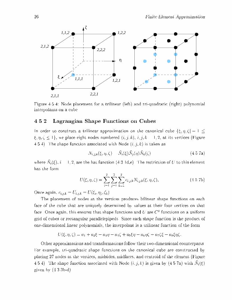
Figure 4.5.4: Node placement for a trilinear (left) and tri-quadratic (right) polynomialinterpolants on a cube.

4.5.2 Lagrangian Shape Functions on Cubes

In order to construct a trilinear approximation on the canonical cube f�; �; �j � 1 ��; �; � � 1g, we place eight nodes numbered (i; j; k), i; j; k = 1; 2, at its vertices (Figure

4.5.4). The shape function associated with Node (i; j; k) is taken as

Ni;j;k(�; �; �) = �Ni(�) �Nj(�) �Nk(�) (4.5.7a)

where �Ni(�), i = 1; 2, are the hat function (4.3.1d,e). The restriction of U to this element

has the form

U(�; �; �) =2X

i=1

2Xj=1

2Xk=1

ci;j;kNi;j;k(�; �; �); (4.5.7b)

Once again, ci;j;k = Ui;j;k = U(�i; �j; �k).

The placement of nodes at the vertices produces bilinear shape functions on each

face of the cube that are uniquely determined by values at their four vertices on that

face. Once again, this ensures that shape functions and U are C0 functions on a uniform

grid of cubes or rectangular parallelepipeds. Since each shape function is the product of

one-dimensional linear polynomials, the interpolant is a trilinear function of the form

U(�; �; �) = a1 + a2� + a3� + a4� + a5�� + a6�� + a7�� + a8��:

Other approximations and transformations follow their two-dimensional counterparts.

For example, tri-quadratic shape functions on the canonical cube are constructed by

placing 27 nodes at the vertices, midsides, midfaces, and centroid of the element (Figure

4.5.4). The shape function associated with Node (i; j; k) is given by (4.5.7a) with �Ni(�)

given by (4.3.3b-d).


4.5.3 Hierarchical Approximations

As with the two-dimensional hierarchical approximations described in Section 4.4, we use

Szab�o and Babu�ska's [7] shape function with the representation of Shephard et al. [6].

The basis for a tetrahedral or a canonical cube begins with the vertex functions (4.5.1)

or (4.5.7), respectively. As noted in Section 4.4, higher-order shape functions are written

as products

Nki (x; y; z) = ��k(�; �; �)�i(�; �; �) (4.5.8)

of an entity function ��k and a blending function �i.

� The entity function is de�ned on a mesh entity (vertex, edge, face, or element) and

varies with the degree k of the approximation. It does not depend on the shapes

of higher-dimensional entities.

� The blending function distributes the entity function over higher-dimensional enti-

ties. It depends on the shapes of the higher-dimensional entities but not on k.

The entity functions that are used to construct shape functions for cubic and tetra-

hedral elements follow.

Edge functions for both cubes and tetrahedra are given by (4.4.6c) and (4.4.2e) as

��k(�) =

p2(2k � 1)

1� �2

Z �

�1

Pk�1(�)d�; k � 2; (4.5.9a)

where � 2 [�1; 1] is a coordinate on the edge. The �rst four edge functions are presented

in (4.4.8).

Face functions for squares are given by (4.4.3) divided by the square face blending

function (4.4.3a)

��k;�;�(�; �) = P�(�)P�(�); �+ � = k � 4; k � 4: (4.5.9b)

Here, (�; �) are canonical coordinates on the face. The �rst six square face functions are

��4;0;0 = 1; ��5;1;0 = �;

��5;0;1 = �; ��6;2;0 =3�2 � 1

2;

��6;1;1 = ��; ��6;0;2 =3�2 � 1

2:

Face functions for triangles are given by (4.4.9) divided the triangular face blending

function (4.4.9a)

��k;�;�(�1; �2; �3) = P�(�2 � �1)P�(2�3 � 1); �+ � = k � 3; k � 3: (4.5.9c)


As with square faces, (�1; �2; �3) form a canonical coordinate system on the face. The

�rst six triangular face functions are

��3;0;0 = 1; ��4;1;0 = �2 � �1;

��4;0;1 = 2�3 � 1; ��5;2;0 =3(�2 � �1)

2 � 1

2;

��5;1;1 = (�2 � �1)(2�3 � 1); ��5;0;2 =3(2�3 � 1)2 � 1

2:

Now, let's turn to the blending functions.

The tetrahedral element blending function for an edge is

�ij(�1; �2; �3; �4) = �i�j (4.5.10a)

when the edge is directed from Vertex i to Vertex j. Using either Figure 4.5.2 or Figure

4.5.3 as references, we see that the blending function ensures that the shape function

vanishes on the two faces not containing the edge to maintain continuity. Thus, if i = 1

and j = 2, the blending function for Edge (1; 2) (which is marked with a 5 on the left of

Figure 4.5.3) vanishes on the faces �1 = 0 (Face A234) and �2 = 0 (Face A134).

The blending function for a face is

�ijk(�1; �2; �3; �4) = �i�j�k (4.5.10b)

when the vertices on the face are i, j, and k. Again, the blending function ensures that

the shape function vanishes on all faces but Aijk. Again referring to Figures 4.5.2 or

4.5.3, the blending function �123 vanishes when �1 = 0 (Face A234), �2 = 0 (Face A134),

and �3 = 0 (Face A124).

The cubic element blending function for an edge is more di�cult to write with our

notation. Instead of writing the general result, let's consider an edge parallel to the �

axis. Then

�1�2;j;k(�; �; �) =1� �2

4�Nj(�) �Nk(�): (4.5.11a)

The factor (1� �2)=4 adjusts the edge function to (4.5.9) as described in the paragraph

following (4.4.9). The one-dimensional shape functions �Nj(�) and �Nk(�) ensure that the

shape function vanishes on all faces not containing the edge. Blending functions for other

edges are obtained by cyclic permutation of �, �, and � and the index. Thus, referring

to Figure 4.5.4, the edge function for the edge connecting vertices 2; 1; 1 and 2; 2; 1 is

�2;1�2;1(�; �; �) =1� �2

4�N2(�) �N1(�):

Since �N2(�1) = 0 (cf. (4.5.7b)), the shape function vanishes on the rear face of the cube

shown in Figure 4.5.4. Since �N1(1) = 0, the shape function vanishes on the top face of


the cube of Figure 4.5.4. Finally, the shape function vanishes at � = �1 and, hence, on

the left and right faces of the cube of Figure 4.5.4. Thus, the blending function (4.5.11a)

has ensured that the shape function vanishes on all but the bottom and front faces of

the cube of Figure 4.5.4.

The cubic face blending function for a face perpendicular to the � axis is

�i;j;k(�; �; �) = �Ni(�)(1� �2)(1� �2): (4.5.11b)

Referring to Figure 4.5.4, the quadratic terms in � and � ensure that the shape func-

tion vanishes on the right, left (� = �1), top, and bottom (� = �1) faces. The one-

dimensional shape function �Ni(�) vanishes on the rear (� = �1) face when i = 1 and on

the front (� = 1) face when i = 2; thus, the shape function vanishes on all faces but the

one to which it is associated.

Finally, there are elemental shape functions. For tetrahedra, there are (p � 1)(p �2)(p� 3)=6 elemental functions for p � 4 that are given by

Nk;�;�;�0 (�1; �2; �3; �4) = �1�2�3�4P�(�2 � �1)P�(2�3 � 1)P�(2�4 � 1);

8 �+ �+ � = k � 4; k = 4; 5; : : : ; p: (4.5.12a)

The subscript 0 is used to identify the element's centroid. The shape functions vanish

on all element faces as indicated by the presence of the multiplier �1�2�3�4. We could

also split this function into the product of an elemental function involving the Legendre

polynomials and the blend involving the product of the tetrahedral coordinates. However,

this is not necessary.

For p � 6 there are the following elemental shape functions for a cube

Nk;�;�;�0 (�; �; �) = (1� �2)(1� �2)(1� �2)P�(�)P�(�)P�(�); 8 �+ �+ � = k � 6:

(4.5.12b)

Again, the shape function vanishes on all faces of the element to maintain continuity.

Adding, we see that there are (p�5)+(p�4)+(p�3)+=6 element modes for a polynomial

of order p.

Shephard et al. [6] also construct blending functions for pyramids, wedges, and prisms.

They display several shape functions and also present entity functions using the basis of

Carnevali et al. [4].

Problems

1. Construct the shape functions associated with a vertex, an edge, and a face node

for a cubic Lagrangian interpolant on the tetrahedron shown on the right of Figure

4.5.3. Express your answer in the tetrahedral coordinates (4.5.3).


��

��

��

��

��

��

��

��

��

��

��

��

1 (x ,y )

y

x

1 1

1 (0,0) 2 (1,0)

3 (0,1)

ξ

η

2 (x ,y )2 2

3 (x ,y )3 3

h

h

h

α

α

α1

1

2

3

2 3

Figure 4.6.1: Nomenclature for a �nite element in the physical (x; y)-plane and for itsmapping to a canonical element in the computational (�; �)-plane.

4.6 Interpolation Error Analysis

We conclude this chapter with a brief discussion of the errors in interpolating a function u

by a piecewise polynomial function U . This work extends our earlier study in Section 2.6

to multi-dimensional situations. Two- and three-dimensional interpolation is, naturally,

more complex. In one dimension, it was su�cient to study limiting processes where mesh

spacings tend to zero. In two and three dimensions, we must also ensure that element

shapes cannot be too distorted. This usually means that elements cannot become too

thin as the mesh is re�ned. We have been using coordinate mappings to construct

bases. Concentrating on two-dimensional problems, the coordinate transformation from

a canonical element in, say, the (�; �)-plane to an actual element in the (x; y)-plane must

be such that no distorted elements are produced.

Let's focus on triangular elements and consider a linear mapping of a canonical unit,

right, 45� triangle in the (�; �)-plane to an element e in the (x; y)-plane (Figure 4.6.1).

More complex mappings will be discussed in Chapter 5. Using the transformation (4.2.8)

to triangular coordinates in combination with the de�nitions (4.2.6) and (4.2.7) of the

canonical variables, we have

24 x

y1

35 =

24 x1 x2 x3

y1 y2 y31 1 1

3524 �1�2�3

35 =

24 x1 x2 x3

y1 y2 y31 1 1

3524 1� � � �

��

35 : (4.6.1)

The Jacobian of this transformation is

Je :=

�x� x�y� y�

�: (4.6.2a)


Di�erentiating (4.6.1), we �nd the determinant of this Jacobian as

det(Je) = (x2 � x1)(y3 � y1)� (x3 � x1)(y2 � y1): (4.6.2b)

Lemma 4.6.1. Let he be the longest edge and �e be the smallest angle of Element e,

then

h2e2sin�e � det(Je) � h2e sin�e: (4.6.3)

Proof. Label the vertices of Element e as 1, 2, and 3; their angles as �1 � �2 � �3; and

the lengths of the edges opposite these angles as h1, h2, and h3 (Figure 4.6.1). With

�1 = �e being the smallest angle of Element e, write the determinant of the Jacobian as

det(Je) = h2h3 sin�e:

Using the law of sines we have h1 � h2 � h3 = he. Replacing h2 by h3 in the above

expression yields the right-hand inequality of (4.6.3). The triangular inequality gives

h3 < h1 + h2. Thus, at least one edge, say, h2 > h3=2. This yields the left-hand

inequality of (4.6.3).

Theorem 4.6.1. Let �(x; y) 2 Hs(e) and ~�(�; �) 2 Hs(0) be such that �(x; y) =~�(�; �) where e is the domain of element e and 0 is the domain of the canonical element.

Under the linear transformation (4.6.1), there exist constants cs and Cs, independent of

�, ~�, he, and �e such that

cs sins�1=2 �eh

s�1e j�js;e

� j~�js;0 � Cs sin�1=2 �eh

s�1e j�js;e

(4.6.4a)

where the Sobolev seminorm is

j�j2s;e=Xj�j=s

ZZe

(D��)2dxdy (4.6.4b)

with D�u being a partial derivative of order j�j = s (cf. Section 3.2).

Proof. Let us begin with s = 0, whereZZe

�2dxdy = det(Je)

ZZ0

~�2d�d�

or

j�j20;e= det(Je)j~�j20;0 :

Dividing by det(Je) and using (4.6.3)

j�j20;e

sin�eh2e� j~�j20;0 �

2j�j20;e

sin�eh2e:


Taking a square root, we see that (4.6.4a) is satis�ed with c0 = 1 and C0 =p2.

With s = 1, we use the chain rule to get

�x = ~��x + ~��x; �y = ~��y + ~��y:

Then,

j�j21;e=

ZZe

(�2x + �2y)dxdy = det(Je)

ZZ0

(g1;e~�2� + 2g2;e~�� ~�� + g3;e~�

2�)d�d�

where

g1;e = �2x + �2y ; g2;e = �x�x + �y�y; g3;e = �2x + �2y:

Applying the inequality ab � (a2 + b2)=2 to the center term on the right yields

j�j21;e � det(Je)

ZZ0

[g1;e~�2� + g2;e(~�

2� +

~�2�) + g3;e~�2�]d�d�:

Letting

� = max(jg1;e + g2;ej; jg3;e + g2;ej)and using (4.6.4b), we have

j�j21;e� det(Je)�j~�j21;0: (4.6.5a)

Either by using the chain rule above with � = x and y or by inverting the mapping

(4.6.1), we may show that

�x =y�

det(Je); �y = � x�

det(Je); �x = � y�

det(Je); �y = � x�

det(Je):

From (4.6.2), jx�j, jx�j, jy�j, jy�j � he; thus, using (4.6.3), we have j�xj, j�yj, j�xj, j�yj �2=(he sin�e). Hence,

� � 16

(he sin�e)2:

Using this result and (4.6.3) with (4.6.5a), we �nd

j�j21;e� 16

sin�ej~�j21;0: (4.6.5b)

Hence, the left-hand inequality of (4.6.4a) is established with c1 = 1=4.

To establish the right inequality, we invert the transformation and proceed from 0

to e to obtain

j~�j21;0 �~�j�j21;e

det(Je)(4.6.6a)


with

~� = max(j~g1;e + ~g2;ej; j~g3;e + ~g2;ej);

~g1;e = x2� + x2�; ~g2;e = x�y� + x�y�; ~g3;e = y2� + y2�:

We've indicated that jx�j, jx�j, jy�j, jy�j � he. Thus, ~� � 4h2e and, using (4.6.3), we �nd

j~�j21;0 �8

sin�e

j�j21;e: (4.6.6b)

Thus, the right inequality of (4.6.4b) is established with C1 = 2p2.

The remainder of the proof follows the same lines and is described in Axelsson and

Barker [2].

With Theorem 4.6.1 established, we can concentrate on estimating interpolation errors

on the canonical triangle. For simplicity, we'll use the Lagrange interpolating polynomial

~U(�; �) =nX

j=1

~u(�j; �j)Nj(�; �); (4.6.7)

with n being the number of nodes on the standard triangle. However, with minor alter-

ations, the results apply to other bases and, indeed, other element shapes. We proceed

with one preliminary theorem and then present the main result.

Theorem 4.6.2. Let p be the largest integer for which the interpolant (4.6.7) is exact

when ~u(�; �) is a polynomial of degree p. Then, there exists a constant C > 0 such that

j~u� ~U js;0 � Cj~ujp+1;0; 8u 2 Hp+1(0); s = 0; 1; : : : ; p+ 1: (4.6.8)

Proof. The proof utilizes the Bramble-Hilbert Lemma and is presented in Axelsson and

Barker [2].

Theorem 4.6.3. Let be a polygonal domain that has been discretized into a net of

triangular elements e, e = 1; 2; : : : ; N�. Let h and � denote the largest element edge

and smallest angle in the mesh, respectively. Let p be the largest integer for which (4.6.7)

is exact when ~u(�; �) is a complete polynomial of degree p. Then, there exists a constant

C > 0, independent of u 2 Hp+1 and the mesh, such that

ju� U js � Chp+1�s

[sin�]sjujp+1; 8u 2 Hp+1(); s = 0; 1: (4.6.9)

Remark 1. The results are restricted s = 0; 1 because, typically, U 2 H1 \Hp+1.


Proof. Consider an element e and use the left inequality of (4.6.4a) with � replaced by

u� U to obtain

ju� U j2s;e� c�2s sin�2s+1 �eh

�2s+2e j~u� ~U j2s;0:

Next, use (4.6.8)


�2s+2e Cj~uj2p+1;0:

Finally, use the right inequality of (4.6.4a) to obtain


�2s+2e CC2

p+1 sin�1 �eh

2pe juj2p+1;e

:

Combining the constants

ju� U j2s;e� C sin�2s �eh

2(p+1�s)e juj2p+1;e

:

Summing over the elements and taking a square root gives (4.6.9).

A similar result for rectangles follows.

Theorem 4.6.4. Let the rectangular domain be discretized into a mesh of rectangular

elements e, e = 1; 2; : : : ; N�. Let h and � denote the largest element edge and smallest

edge ratio in the mesh, respectively. Let p be the largest integer for which (4.6.7) is exact

when ~u(�; �) is a complete polynomial of degree p. Then, there exists a constant C > 0,

independent of u 2 Hp+1 and the mesh, such that

ju� U js � Chp+1�s

�sjujp+1; 8u 2 Hp+1(); s = 0; 1: (4.6.10)

Proof. The proof follows the lines of Theorem 4.6.3 [2].

Thus, small and large (near �) angles in triangular meshes and small aspect ratios

(the minimum to maximum edge ratio of an element) � in a rectangular mesh must be

avoided. If these quantities remain bounded then the mesh is uniform as expressed by

the following de�nition.

De�nition 4.6.1. A family of �nite element meshes �h is uniform if all angles of all

elements are bounded away from 0 and � and all aspect ratios are bounded away from

zero as the element size h! 0.

With such uniform meshes, we can combine Theorems 4.6.2, 4.6.3, and 4.6.4 to obtain

a result that appears more widely in the literature.

Theorem 4.6.5. Let a family of meshes �h be uniform and let the polynomial inter-

polant U of u 2 Hp+1 be exact whenever u is a complete polynomial of degree p. Then

there exists a constant C > 0 such that

ju� U js � Chp+1�sjujp+1; s = 0; 1: (4.6.11)


Proof. Use the bounds on � and � with (4.6.9) and (4.6.10) to rede�ne the constant C

and obtain (4.6.11).

Theorems 4.6.2 - 4.6.5 only apply when u 2 Hp+1. If u has a singularity and belongs

to Hq+1, q < p, then the convergence rate is reduced to

ju� U js � Chq+1�sjujq+1; s = 0; 1: (4.6.12)

Thus, there appears to be little bene�t to using p th-degree piecewise-polynomial inter-

polants in this case. However, in some cases, highly graded nonuniform meshes can be

created to restore a higher convergence rate.

Bibliography

[1] S. Adjerid, M. Ai�a, and J.E. Flaherty. Hierarchical �nite element bases for triangular

and tetrahedral elements. Computer Methods in Applied Mechanics and Engineering,

2000. to appear.

[2] O. Axelsson and V.A. Barker. Finite Element Solution of Boundary Value Problems.

Academic Press, Orlando, 1984.

[3] S.C. Brenner and L.R. Scott. The Mathematical Theory of Finite Element Methods.

Springer-Verlag, New York, 1994.

[4] P. Carnevali, R.V. Morric, Y.Tsuji, and B. Taylor. New basis functions and com-

putational procedures for p-version �nite element analysis. International Journal of

Numerical Methods in Enginneering, 36:3759{3779, 1993.

[5] S. Dey, M.S. Shephard, and J.E. Flaherty. Geometry-based issues associated with

p-version �nite element computations. Computer Methods in Applied Mechanics and

Engineering, 150:39 { 50, 1997.

[6] M.S. Shephard, S. Dey, and J.E. Flaherty. A straightforward structure to construct

shape functions for variable p-order meshes. Computer Methods in Applied Mechanics

and Engineering, 147:209{233, 1997.

[7] B. Szab�o and I. Babu�ska. Finite Element Analysis. John Wiley and Sons, New York,

1991.

[8] O.C. Zienkiewicz. The Finite Element Method. McGraw-Hill, New York, third edition,

1977.

37

chapter · chapter 4 finite elemen t appro ximation 4.1 in tro duction our goal in this c hapter is...

Documents