4 gis methods and considerations - pdana.com · rome as computed in longitude/latitude space and in...

This chapter describes the processes used to estimate the spatial and temporal distribution of settlement sites at Metaponto in a Geographic Information Systems (GIS) environment. An artifact database was linked to layers of spatially referenced information and subjected to various spatial analyses, resulting in a series of displays of settlement patterns by period over the study area. The materials available for analy-sis included a relational artifact database containing almost 11,000 records, a set of point and polygon GIS layers describing the positions of sites and plots, and a set of supporting GIS layers consisting of streams, elevations, geomorphological features, and scanned maps and aerial photographs. The study area in this volume, that part of the chora of Metaponto between the Bradano and Basento Rivers in southern Italy, covers an area of ca. 10,000 hectares at approximately 16° 45′ east longitude and 40° 25′ north latitude.

Microsoft Access and Excel, ESRI’s ArcGIS, Golden Software’s Surfer, The MathWorks’ MatLab, and the SPSS Graduate Pack were used for the analyses. Most processing was done within the Universal Transverse Mercator (UTM) coordinate system. Other coordi-nate systems were tested and used where appropriate. The GIS platform was tested for its ability to handle the coordinate systems and geographic operators. Site locations were dated using fine-ware artifacts. Date periods were established, and a series of dates representing periods of maximum site occupation were computed. Sites were categorized into types, such as farmhouses, tombs, sanctuaries, and others. Error analysis and quality control were monitored throughout the project. The results of this process consist of estimates of spatial and temporal change in settlement patterns based on the ensemble of artifacts for sites identified as farm sites.

4GIS Methods and Considerations

Peter H. Dana

Figure 4.1 Metaponto study area regions for GIS analysis. (PD)

94 Peter H. Dana

Source MaterialsA Microsoft Access database table consisting of 10,995 records, created by the various artifact specialists who contributed to the project, forms the basis for this study. Each record is labeled with the number of the site or survey plot where each artifact was found, with chronological information contained in other fields. The geographic attributes of the sites and plots are derived from several sources. Sites 1–787 were imported into the GIS as an event theme from a data-base of site attributes including northing and easting positions, which were read from the original 1:10,000 topographic sheets employed in the field campaigns. Sites 793–800 were located using a Global Position-ing System receiver with differential correction ca-pability. Plot boundaries were either digitized from scanned field maps (1993–1999) or traced with the GPS receiver (2000–2001). Elevation data is recorded in at least one of four sources: a Digital Elevation Model (DEM) of the Metaponto study area generated from Shuttle Radar Topography Mission (SRTM) data, elevation contour polygons of the study area digitized from the 1:10,000 topographic maps, individual site location elevations read from the 1:10,000 topographic maps, and GPS readings for sites documented in 2000–2001. Hydrology data, consisting of natural streams and man-made canals, were digitized from the 1:10,000 topographic maps and from the Istituto Geografico Militare (IGM)’s 1:50,000 topographic maps (sheets 491/Ferrandina, 492/Ginosa, and 508/Policoro). James T. Abbott’s geomorphological map of the chora pre-pared from aerial photographs was digitized to obtain the geomorphological data.

Study AreaWe defined the study area at its largest extent by the chora of Metaponto. This region contains all the surveyed plots and sites in the Metapontino from the Bradano to Cavone Rivers. For this volume we con-fined the study area to that part of the chora north of the Basento River. We then decided to restrict analysis further through the creation of a 200-m buffer around all the sites and plots north of the Basento that can be dated with fine-ware artifacts. Our most restrictive definition of the study area is defined by a 50-m buffer around dateable locations north of the Basento. These various study area polygons are depicted in Fig. 4.1.

Analysis PlatformsWe began the project with ESRI’s ArcGIS version 8.3 and finished with version 9.3. Most spatial analysis and all graphic display of analysis results were performed in ArcMap, the kernel ArcGIS module. We used The MathWorks’ MatLab programming environment to produce custom data files and to perform cluster analysis using algorithms developed by the author. We employed SPSS as a platform for several statistical analysis procedures that were essentially non-spatial.

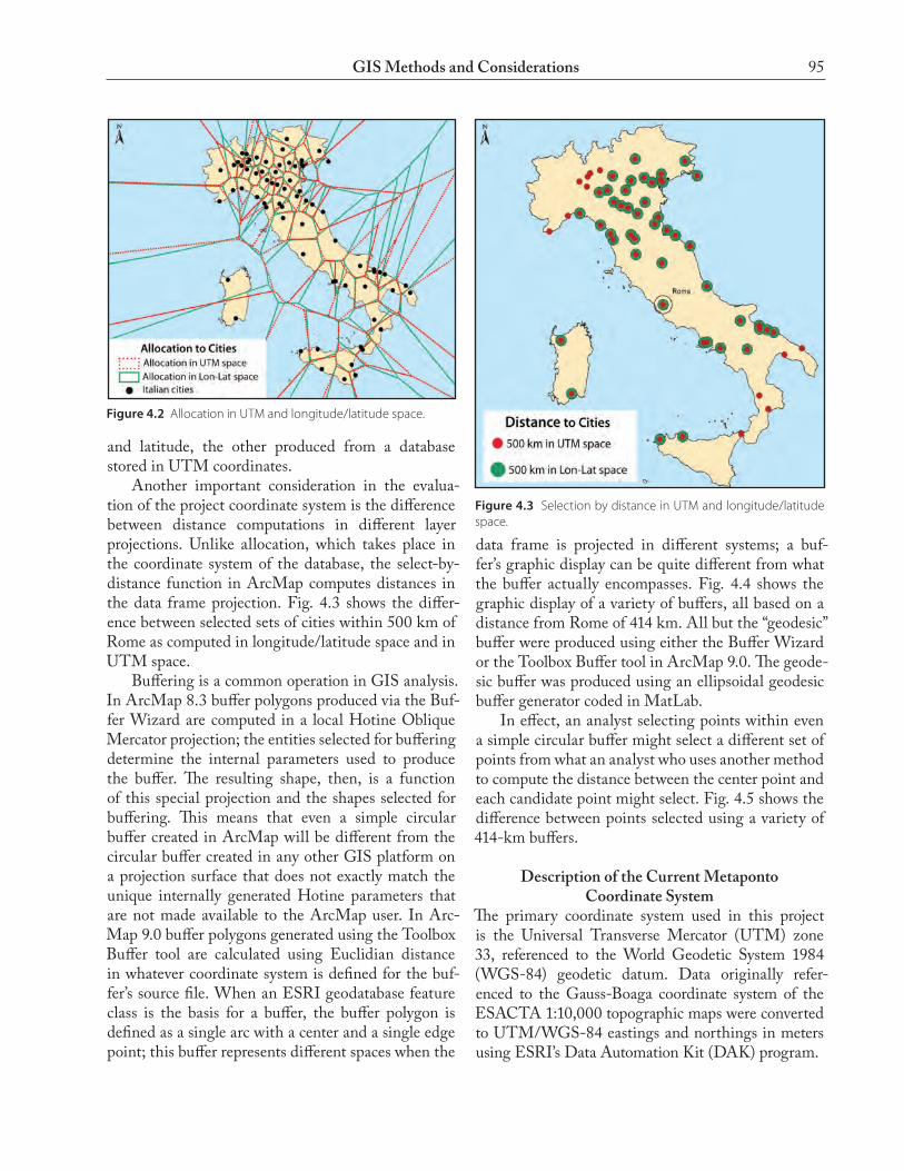
Coordinate Systems and Spatial AnalysisThe coordinate system used for GIS analysis can have profound effects on that analysis. For the definition of single points on the surface of the earth any coor-dinate system that allows for the conversion to and from longitude, latitude, and height with reference to a specific geodetic datum can be used for accurate portrayal of position. Surveyors and geodesists make use of numerical methods for computing distance and azimuths along specified paths between points with reference to an ellipsoidal earth surface. GIS platforms, however, use a variety of methods for the computation of distances and angles. Distances and angles, as well as quantities derived from them such as area, aspect, slope, and stream sinuosity, are often used within GIS spatial analysis processes. GIS platforms rarely use geodetic computational methods (I know of none that do); rather, they use simple and fast operations, often based on Pythagorean methods and simple trigono-metric functions on the surface of a plane. The plane on which these calculations are performed varies between platforms, databases, and specific functions. ESRI’s ArcMap is a typical GIS platform. Under different circumstances ArcMap computes the dis-tance between points and angles from one point to another in significantly different ways. If one takes a database of points such as the major cities of Italy and produces a proximity (allocation) grid, the com-putations take place in the coordinate system of the original database, irrespective of the display projec-tion of the data frame within which the allocation is performed. Allocation assigns to each cell in a grid the value of the point closest to it. Different allocation grids are produced depending on the coordinate sys-tem of the database representing the points. Fig. 4.2 shows two sets of allocation polygons, one produced from a database of Italian cities stored in longitude


Figure 4.2 Allocation in UTM and longitude/latitude space.

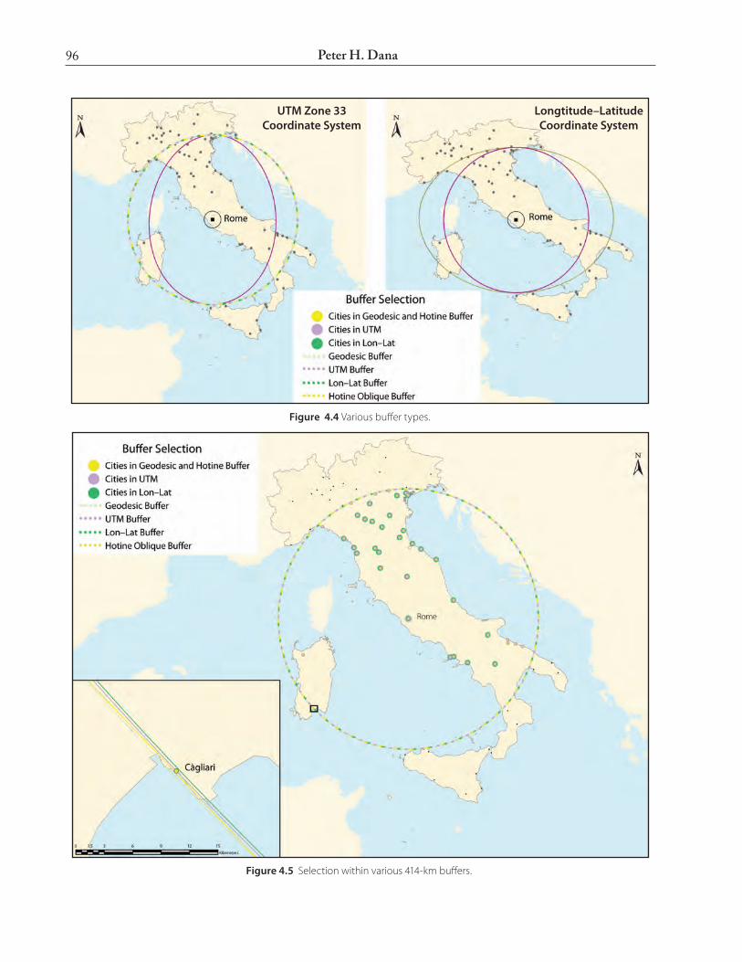
Figure 4.3 Selection by distance in UTM and longitude/latitude space.

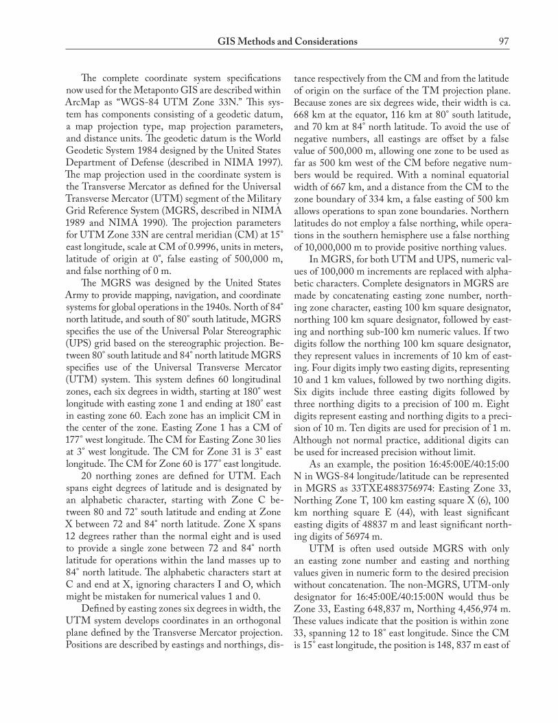
and latitude, the other produced from a database stored in UTM coordinates. Another important consideration in the evalua-tion of the project coordinate system is the difference between distance computations in different layer projections. Unlike allocation, which takes place in the coordinate system of the database, the select-by-distance function in ArcMap computes distances in the data frame projection. Fig. 4.3 shows the differ-ence between selected sets of cities within 500 km of Rome as computed in longitude/latitude space and in UTM space. Buffering is a common operation in GIS analysis. In ArcMap 8.3 buffer polygons produced via the Buf-fer Wizard are computed in a local Hotine Oblique Mercator projection; the entities selected for buffering determine the internal parameters used to produce the buffer. The resulting shape, then, is a function of this special projection and the shapes selected for buffering. This means that even a simple circular buffer created in ArcMap will be different from the circular buffer created in any other GIS platform on a projection surface that does not exactly match the unique internally generated Hotine parameters that are not made available to the ArcMap user. In Arc-Map 9.0 buffer polygons generated using the Toolbox Buffer tool are calculated using Euclidian distance in whatever coordinate system is defined for the buf-fer’s source file. When an ESRI geodatabase feature class is the basis for a buffer, the buffer polygon is defined as a single arc with a center and a single edge point; this buffer represents different spaces when the

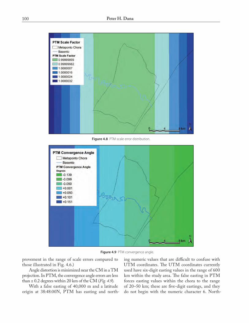
data frame is projected in different systems; a buf-fer’s graphic display can be quite different from what the buffer actually encompasses. Fig. 4.4 shows the graphic display of a variety of buffers, all based on a distance from Rome of 414 km. All but the “geodesic” buffer were produced using either the Buffer Wizard or the Toolbox Buffer tool in ArcMap 9.0. The geode-sic buffer was produced using an ellipsoidal geodesic buffer generator coded in MatLab. In effect, an analyst selecting points within even a simple circular buffer might select a different set of points from what an analyst who uses another method to compute the distance between the center point and each candidate point might select. Fig. 4.5 shows the difference between points selected using a variety of 414-km buffers.

Description of the Current MetapontoCoordinate System

The primary coordinate system used in this project is the Universal Transverse Mercator (UTM) zone 33, referenced to the World Geodetic System 1984 (WGS-84) geodetic datum. Data originally refer-enced to the Gauss-Boaga coordinate system of the ESACTA 1:10,000 topographic maps were converted to UTM/WGS-84 eastings and northings in meters using ESRI’s Data Automation Kit (DAK) program.

96 Peter H. Dana

Figure 4.5 Selection within various 414-km buffers.

Figure 4.4 Various buffer types.

UTM Zone 33 Coordinate System

Longtitude–Latitude Coordinate System


The complete coordinate system specifications now used for the Metaponto GIS are described within ArcMap as “WGS-84 UTM Zone 33N.” This sys-tem has components consisting of a geodetic datum, a map projection type, map projection parameters, and distance units. The geodetic datum is the World Geodetic System 1984 designed by the United States Department of Defense (described in NIMA 1997). The map projection used in the coordinate system is the Transverse Mercator as defined for the Universal Transverse Mercator (UTM) segment of the Military Grid Reference System (MGRS, described in NIMA 1989 and NIMA 1990). The projection parameters for UTM Zone 33N are central meridian (CM) at 15° east longitude, scale at CM of 0.9996, units in meters, latitude of origin at 0°, false easting of 500,000 m, and false northing of 0 m. The MGRS was designed by the United States Army to provide mapping, navigation, and coordinate systems for global operations in the 1940s. North of 84° north latitude, and south of 80° south latitude, MGRS specifies the use of the Universal Polar Stereographic (UPS) grid based on the stereographic projection. Be-tween 80° south latitude and 84° north latitude MGRS specifies use of the Universal Transverse Mercator (UTM) system. This system defines 60 longitudinal zones, each six degrees in width, starting at 180° west longitude with easting zone 1 and ending at 180° east in easting zone 60. Each zone has an implicit CM in the center of the zone. Easting Zone 1 has a CM of 177° west longitude. The CM for Easting Zone 30 lies at 3° west longitude. The CM for Zone 31 is 3° east longitude. The CM for Zone 60 is 177° east longitude. 20 northing zones are defined for UTM. Each spans eight degrees of latitude and is designated by an alphabetic character, starting with Zone C be-tween 80 and 72° south latitude and ending at Zone X between 72 and 84° north latitude. Zone X spans 12 degrees rather than the normal eight and is used to provide a single zone between 72 and 84° north latitude for operations within the land masses up to 84° north latitude. The alphabetic characters start at C and end at X, ignoring characters I and O, which might be mistaken for numerical values 1 and 0. Defined by easting zones six degrees in width, the UTM system develops coordinates in an orthogonal plane defined by the Transverse Mercator projection. Positions are described by eastings and northings, dis-

tance respectively from the CM and from the latitude of origin on the surface of the TM projection plane. Because zones are six degrees wide, their width is ca. 668 km at the equator, 116 km at 80° south latitude, and 70 km at 84° north latitude. To avoid the use of negative numbers, all eastings are offset by a false value of 500,000 m, allowing one zone to be used as far as 500 km west of the CM before negative num-bers would be required. With a nominal equatorial width of 667 km, and a distance from the CM to the zone boundary of 334 km, a false easting of 500 km allows operations to span zone boundaries. Northern latitudes do not employ a false northing, while opera-tions in the southern hemisphere use a false northing of 10,000,000 m to provide positive northing values. In MGRS, for both UTM and UPS, numeric val-ues of 100,000 m increments are replaced with alpha-betic characters. Complete designators in MGRS are made by concatenating easting zone number, north-ing zone character, easting 100 km square designator, northing 100 km square designator, followed by east-ing and northing sub-100 km numeric values. If two digits follow the northing 100 km square designator, they represent values in increments of 10 km of east-ing. Four digits imply two easting digits, representing 10 and 1 km values, followed by two northing digits. Six digits include three easting digits followed by three northing digits to a precision of 100 m. Eight digits represent easting and northing digits to a preci-sion of 10 m. Ten digits are used for precision of 1 m. Although not normal practice, additional digits can be used for increased precision without limit. As an example, the position 16:45:00E/40:15:00 N in WGS-84 longitude/latitude can be represented in MGRS as 33TXE4883756974: Easting Zone 33, Northing Zone T, 100 km easting square X (6), 100 km northing square E (44), with least significant easting digits of 48837 m and least significant north-ing digits of 56974 m. UTM is often used outside MGRS with only an easting zone number and easting and northing values given in numeric form to the desired precision without concatenation. The non-MGRS, UTM-only designator for 16:45:00E/40:15:00N would thus be Zone 33, Easting 648,837 m, Northing 4,456,974 m. These values indicate that the position is within zone 33, spanning 12 to 18° east longitude. Since the CM is 15° east longitude, the position is 148, 837 m east of

98 Peter H. Dana

the CM (the false easting of 500,000 m is subtracted from the easting to yield the distance from the CM on the TM projection plane). The position is 4,456,974 m from the equator on the projection plane. The same values of easting and northing can be found in each of the 60 UTM easting zones, in exactly the same place on the projection plane with respect to the 60 CM values and the equator.

evaluation of the Current MetapontoCoordinate System

The geodetic datum selected for the current coordi-nate system is perfectly valid for GIS analysis. WGS-84 is a global, earth-centered datum that is generally accepted as an estimate for the size and shape of the Earth, as well as a definition for the origin and ori-entation of coordinate systems. Parameters exist for conversion from many local systems to WGS-84, and, while there are local maps referenced to other datums, the Italian national cartographic agency (IGM) pro-duces maps referenced to WGS-84. UTM is perfectly acceptable for defining point positions on the ground in a coordinate system. Conversion between UTM and other georeferenc-ing systems in use such as longitude/latitude can be accomplished in both forward and inverse senses without loss of accuracy, as long as the methods are selected appropriately. However, the UTM projection plane is only moderately useful for accurate distance, area, and azimuth calculations in a GIS environment. Any Transverse Mercator projection is conformal, i.e., it can represent local shapes accurately because local and relative angular relationships are preserved. The projection is not equidistant, equal-angle, or equal-area.1 TM projections have correct scale only along two lines of longitude equidistant from the CM if the scale factor at the CM is defined as less than one (<1.0). If the scale at the CM is set to 1.0, then scale is correct only along the CM. In the UTM version of the TM projection, the scale at the CM is 0.9996, which forces the lines of correct scale to fall along north-south lines approximately 180 km on either side of the CM. While this distributes scale errors nearly equally within the six-degree zones of the UTM pro-jection, distances computed using simple Pythago-rean methods (square root of the sum of the easting distance squared and the northing distance squared)

1 Snyder 1987.

are always incorrect except along paths where the scale factor averages to 1.0. Azimuthal relationships, while locally and relatively faithful to shapes, are not correct except along the CM. Azimuths computed using simple arctangent methods are subject to the local difference between grid north (the direction of UTM easting lines) and true north (the direction of longitudinal lines). Since distance and direction are everywhere incorrect (except as noted), area computa-tions are erroneous everywhere as well. In the UTM version of the Transverse Mercator projection, scale and azimuth errors can be computed at any point. Thus it is possible to estimate the errors in distance, azimuth, and area that will occur in any local region using simple Pythagorean methods for distance or arctangent methods for azimuths. Com-puting distance or azimuth errors, or correcting for them, over long distances on oblique paths is quite difficult (so difficult that accurate results are really possible only by conversion to longitude/latitude fol-lowed by computation of ellipsoidal geodesic path distances and azimuths). The Metaponto study area can be defined as a region including the chora, sites, and related sites within a bounding rectangle with the following lim-its: 16.40–16.92° east longitude, and 40.1–40.7° north latitude. The UTM grid used within the Metaponto study area experiences scale errors ranging from 0.999772 to 0.99993 (Fig. 4.6). Angle differences between true north and grid north (the convergence angle) vary between 0.9 and 1.2 degrees over the study area (Fig. 4.7).

Alternate Metaponto Coordinate System:The Pantanello Transverse Mercator (PTM)

It is relatively easy to design a coordinate system and implement it in ArcMap. A properly designed system can minimize distortions of distance, angle, shape, and area over the study area. The following coordinate system, designated Pantanello Transverse Mercator (PTM), is an attempt to solve distortion problems in GIS analysis. It has the following parameters: CM at 16.733333 degrees (16°:44′:00″) east longitude, scale at CM of 0.9999990, units in meters, latitude of origin at 38.80° degrees (38°:48′:00″), false easting of 40,000 m, and false northing of 0.0 m. The TM projection is appropriate for a number of reasons. It is familiar to most researchers, used in Italy,


Figure 4.6 UTM scale factor.

Figure 4.7 UTM convergence angle.

and based on UTM. It is often used for regions with longer latitudinal extent than longitudinal extent. It can be designed to minimize scale errors over the region of use and is conformal, thus maintaining local shapes. The CM for PTM has been selected to pass near the center of the study area, at 16:44:00 east longi-tude. The scale of 1/1,000,000 (k = 0.999999) places

the eastings of correct scale (k = 1.0) approximately 10 km east and west of the CM; the scale rises to 1.000004 ca. 20 km east and west of the CM. PTM distributes scale errors over the study area with dis-tance errors of better than one part in one million (1 cm in 100 km). Fig. 4.8 illustrates the scale errors in PTM over the study area. (Note the relative im-

100 Peter H. Dana

provement in the range of scale errors compared to those illustrated in Fig. 4.6.) Angle distortion is minimized near the CM in a TM projection. In PTM, the convergence angle errors are less than ± 0.2 degrees within 20 km of the CM (Fig. 4.9). With a false easting of 40,000 m and a latitude origin at 38:48:00N, PTM has easting and north-

ing numeric values that are difficult to confuse with UTM coordinates. The UTM coordinates currently used have six-digit easting values in the range of 600 km within the study area. The false easting in PTM forces easting values within the chora to the range of 20–50 km; these are five-digit eastings, and they do not begin with the numeric character 6. North-

Figure 4.8 PTM scale error distribution.

Figure 4.9 PTM convergence angle.


ing values in UTM zone 33 within the chora are all seven-digit values in the range of 4400–4500 km, while in PTM the northing values in the chora range from 160–190 km. These are six-digit values, none beginning with 44 or 45. Thus PTM eastings and northings are easily differentiated from each other and from UTM values within the study area.

Advantages of PTM for GIS AnalysisThe primary advantage of PTM is the reduction of UTM scale and angle errors. In all cases, point, line and polygon vertices remain the same with respect to the ground and to other layers in PTM or UTM. With changes in map projection, paths between points may change, and so polygon edges may fall more accurately in the PTM projection. It is in spa-tial analysis that the coordinate system of individual layers or the frame projection makes a difference and where PTM is advantageous. Should analysis and mapping of the Metaponto data be combined with survey-quality data sets, the UTM scale and angle errors would be far too large. UTM scale errors of 1 m in 2500 m at the CM would be reduced to 1 m in 6666 m in PTM at the center of the study area, corresponding to second- or third-order land surveys. PTM scale reductions would result in a maximum error of 1 m in 100,000 m at the

extent of current project mapping. In the chora, the scale errors would be better than one part in 500,000, far exceeding first-order land survey specifications.2

Angular distortion would be minimized near the CM: in UTM errors exceed 1.2 degrees within the study area, but PTM has angular distortions of less than 0.2 degrees at the extent of the study area. The implications of these scale and angle dis-tortions for GIS analysis have been outlined above. Three examples of GIS spatial analysis may help dem-onstrate the improvement in PTM. Allocation (sometimes called “proximity”) is the process of creating a raster grid of cells containing a value corresponding to the nearest feature in a point layer to that grid cell. Allocation results in polygonal areas known as Thiessen or Voronoi polygons.3 The point layer of the survey sites in UTM coordinates results in polygonal regions that differ from those created by the same layer converted to PTM. Since the allocation function operates within the coordinate space of the spatial database, the layer projection has no influence on the process in ArcMap. Fig. 4.10 shows the edge differences between two sets of proximity polygons, one in UTM, the other in PTM.

2 Kavanagh and Bird 2000.3 O’Sullivan and Unwin 2003, 43.

Figure 4.10 Allocation in UTM and PTM space.

102 Peter H. Dana

Note the occurrence of edge disparities between these two sets of polygons ranging from 10 to 100 m. Crucial here is that the scale and angle distortions in the UTM-based polygons have rendered them a less accurate representation of nearest neighbor position than polygons formed in PTM space. Another example is the influence of distance and angle distortion on area and perimeter calculations. The chora extent layer in UTM results in an area computation of 194.807 km2. When converted to PTM, it produces a more accurate result of 194.857 km2. The perimeter length changes too, from a UTM estimate of 60.596 km to a more accurate PTM estimate of 60.604 km. A third example illustrates the direction (angle) errors of the UTM grid within the study area. Fig. 4.11 shows the result of the difference between the computed mean direction for division lines (non-transverse) in the study area. The mean angular difference between the two sets of lines, one projected in UTM coordinates, the other in PTM is 1.2 degrees, the UTM grid convergence error in the study area.

RecommendationsA new GIS data set based on PTM could be introduced in place of the current UTM-based one with minimal effort. Conversion of point, line, and polygon layers from UTM to PTM is a task that can be accomplished in just a few hours. If analysis will never require accu-racy better than 10 m in the horizontal plane or five de-grees of azimuth, conversion may not be necessary. The computational risks in conversion are minimal. On the other hand, a new coordinate system would introduce a complexity that does not now exist. Confusion, while minimized by the specific parameters selected for the proposed PTM system, could result between datasets referenced to UTM and those referenced to PTM. If project researchers decide that survey-quality distance and direction analysis will be required of the Metaponto data set, or that results will be combined with first- or second-order survey data, then this pro-posed coordinate system should be implemented before analysis is begun. Once new raster or vector layers are created in spatial analysis based on values derived from distance or directions, it is too late to make any meaningful conversion. The rule of thumb in GIS analysis is that results are never better than the spatial errors in the least accurate layer. Conversion to PTM

Figure 4.11 Direction differences for non-transverse division lines in the study area.


would insure that future layers resulting from spatial analysis will be the most accurate possible.

GIS Platform TestsBefore implementing the proposed PTM coordinate system, we performed tests to ensure that conversions among longitude/latitude, UTM, and PTM could be accomplished within ArcMap with reasonable accuracy.

Description of the Test Data SetIn MatLab we computed the coordinates of nine points: a position near the center of the study area and eight points equally spaced in geodetic azimuth (45 degrees apart) around the center point. Each point was com-puted at a distance of 10,000 m from the center point on the surface of the WGS-84 ellipsoid using Vincenty’s direct method for producing longitude and latitude at a distance and azimuth from a point (Fig. 4.12).

Coordinate Conversion and ResultsThe numeric values in decimal degrees were converted using methods specified in Snyder (1987) into UTM zone 33 and PTM coordinates. The nine points were then imported into ArcMap and converted to point feature layers using the Display XY Events tool with

the coordinate system defined as WGS-84 with UTM and PTM. The Toolbox Project utility was used to convert the longitude/latitude layer into a UTM zone 33N/WGS-84 layer and a PTM layer. Comparison showed that the PTM eastings and northings differ by less than 1 cm from the Snyder/MatLab coordinates, and the UTM eastings and northings differ by less than 1 dm (decimeter). The difference in the values is insignificant for any poten-tial use of ICA’s Metaponto data sets in GIS analysis. Of course, conversion to PTM, as helpful as it may be for accurate spatial analysis, is of little use if results cannot be exported as GIS layers in other formats. To insure that conversion using the Toolbox and the Pro-jection wizard works equally well in both the forward and inverse directions, the point files in UTM and PTM were converted back to longitude/latitude in new layers. In addition, the PTM file was converted to UTM. In all cases the Toolbox conversions match the original longitude/latitude points and the UTM points to better than 1 cm.

Figure 4.12 Nine test points within the study area.

104 Peter H. Dana

Location DatingWe decided to date sites and plots solely by the fine-ware pottery. The first step in the process was to as-sign the dates provided by the artifact specialists to the sites and plots. All records for fine-ware artifacts were extracted from the master artifact database. The survey plots were converted to point features by computing a centroid X/Y value for each polygon, and these centroids were added to the database of site positions to create a new layer containing all locations. The location layer and fine-ware artifact database were then joined in ArcMap to give the artifacts geo-graphic locations.

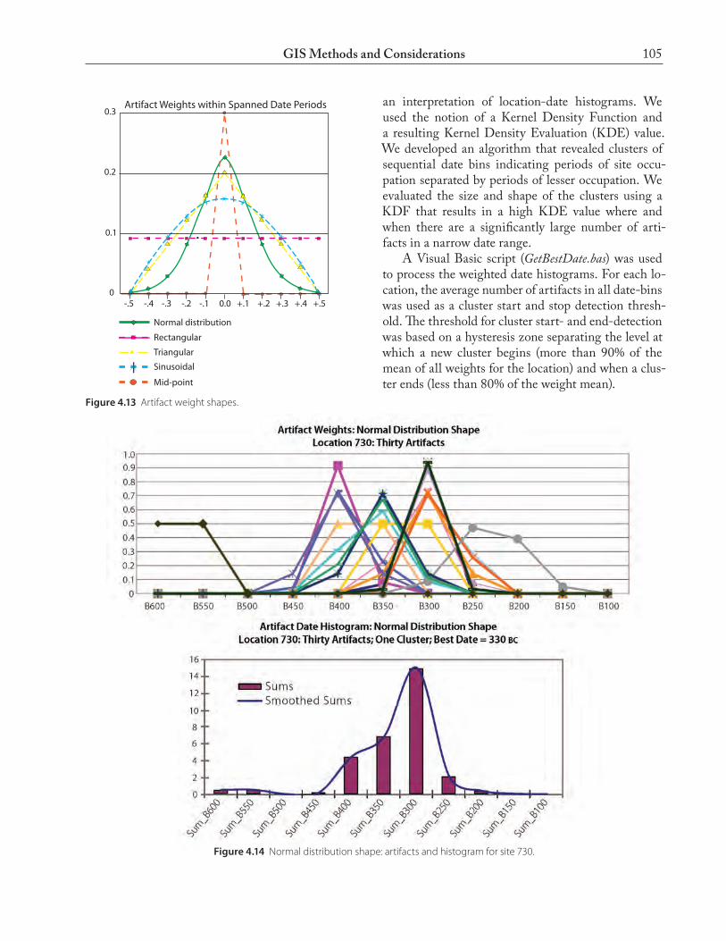
Artifact Date Range ProcessingWe then tested the differences between sites and site revisit polygons and decided that plot polygons and original site locations (not revisit locations) represent the best point locations for all artifacts. We produced date histograms for each location based on the ensemble of dated artifacts found at each site. We computed histogram values for twelve date bins, each spanning fifty years, through the range from 625 BC to 25 BC. For example the 400 BC bin would contain the relative number of artifacts with date ranges falling within years more than or equal to 375 BC to less than 425 BC. We first adjusted each artifact date by adding twenty years to each end of the artifact date span, to account for the uncertainty of artifact dating. We experimented with weighting of individual artifacts in an attempt to allow more weight to the center of an artifact date range without using a simple mid-point date to dominate the histogram for all artifacts at a location. We computed individual artifact weights based on mid-point, rectangular, triangular, sinusoidal, and normal distribution curve shapes. After consultation with experts (see Dana 2004) we settled on the shape of a normal distribution curve that concentrated most of the weight near the mid-point of the assigned date range. We divided each artifact’s extended date range by six and used the normal distribution curve cumulative probability function to assign 68% of the artifact weight in the middle third of the range, 27% to the third of the range beyond the middle third, and 5% to the outer third of the range.

The cumulative probability function we used is a numerical solution to the integral method:4

Public Function pnorm(x) Dim t As Double Dim dblQ As Double Dim pi As Double Dim fx As Double lngFeatureCount = 0 pi=4 * Atn(1)‘ Calculate the value of pi.

t=1# / (1# + Abs(x) * 0.2316419) fx=1 / Sqr(2 * pi) * Exp(-x ^ 2 / 2) dblQ = fx * (0.31938153 * t - 0.356563782 * t ^ 2 + 1.781477937 * t ^ 3 - 1.821255978 * t ^ 4 + 1.330274429 * t ^ 5) If x > 0 Then dblQ = 1# - dblQ End If pnorm = dblQEnd Function

The artifact weights are computed using a Visual Basic for Applications (VBA) script, ProcessDates.bas. The script allows the selection of any of the weighting mechanisms, and results in an artifact list with weights in each of the fifty-year date ranges for each artifact. Fig. 4.13 shows the five different weighting methods. All the dated artifacts found at each location con-tribute to fifty-year date histogram bins for that loca-tion. Each bin is the result of summing the weights for each artifact of which the extended date range spans a date bin. The resulting sums are normalized to equivalent numbers of artifacts because each arti-fact weight is normalized to 1.0 over its date range through the cumulative probability function. Each location date bin represents the equivalent number of artifacts found at a location with a weighted date range within that fifty-year span. Fig. 4.14 shows the artifact weights and the resulting histogram bin sums for location 730.

Location Dating Analysis (“Best Date”)We asked several questions based on dated artifacts and their locations: When was a location occupied? When was the period of maximum occupation? Was the location occupied over a long period or a short period? Was the location occupied at different periods with intervening periods of lesser occupation? To help answer these questions we took an ap-proach that allowed us to weight evidence based on

4 Abramowitz and Stegun 1968; Hewlett Packard 1974


an interpretation of location-date histograms. We used the notion of a Kernel Density Function and a resulting Kernel Density Evaluation (KDE) value. We developed an algorithm that revealed clusters of sequential date bins indicating periods of site occu-pation separated by periods of lesser occupation. We evaluated the size and shape of the clusters using a KDF that results in a high KDE value where and when there are a significantly large number of arti-facts in a narrow date range. A Visual Basic script (GetBestDate.bas) was used to process the weighted date histograms. For each lo-cation, the average number of artifacts in all date-bins was used as a cluster start and stop detection thresh-old. The threshold for cluster start- and end-detection was based on a hysteresis zone separating the level at which a new cluster begins (more than 90% of the mean of all weights for the location) and when a clus-ter ends (less than 80% of the weight mean).

Figure 4.13 Artifact weight shapes.

Figure 4.14 Normal distribution shape: artifacts and histogram for site 730.

Normal distribution

Rectangular

Triangular

Sinusoidal

Mid-point

Artifact Weights within Spanned Date Periods

0.1

0.2

0.3

0-.5 -.4 -.3 -.2 -.1 0.0 +.1 +.2 +.3 +.4 +.5

106 Peter H. Dana

The number of bins and the number of artifacts in each cluster was computed. This process resulted in one to four possible artifact date clusters for each loca-tion. Two weights were computed for each cluster. A number-of-artifacts weight was computed as a value from 0.0 to 1.0 formed by the ratio of artifacts in each cluster to the number of artifacts found at each location. A deviation-weight was computed from the reciprocal of the number of date-bins in each cluster. For each date cluster a cluster-weight (the KDE value) was computed by multiplying the number-of-artifacts weight by the deviation-weight. For a date where all the artifacts fell within a single bin, the resulting weight was 1.0. The date cluster with the highest KDE was selected as the “best date” cluster. The “best date” is the mean date for bins within the

highest KDE cluster. This “best date” is an estimate for the date of maximum site occupation based on all dated artifacts found at the site.

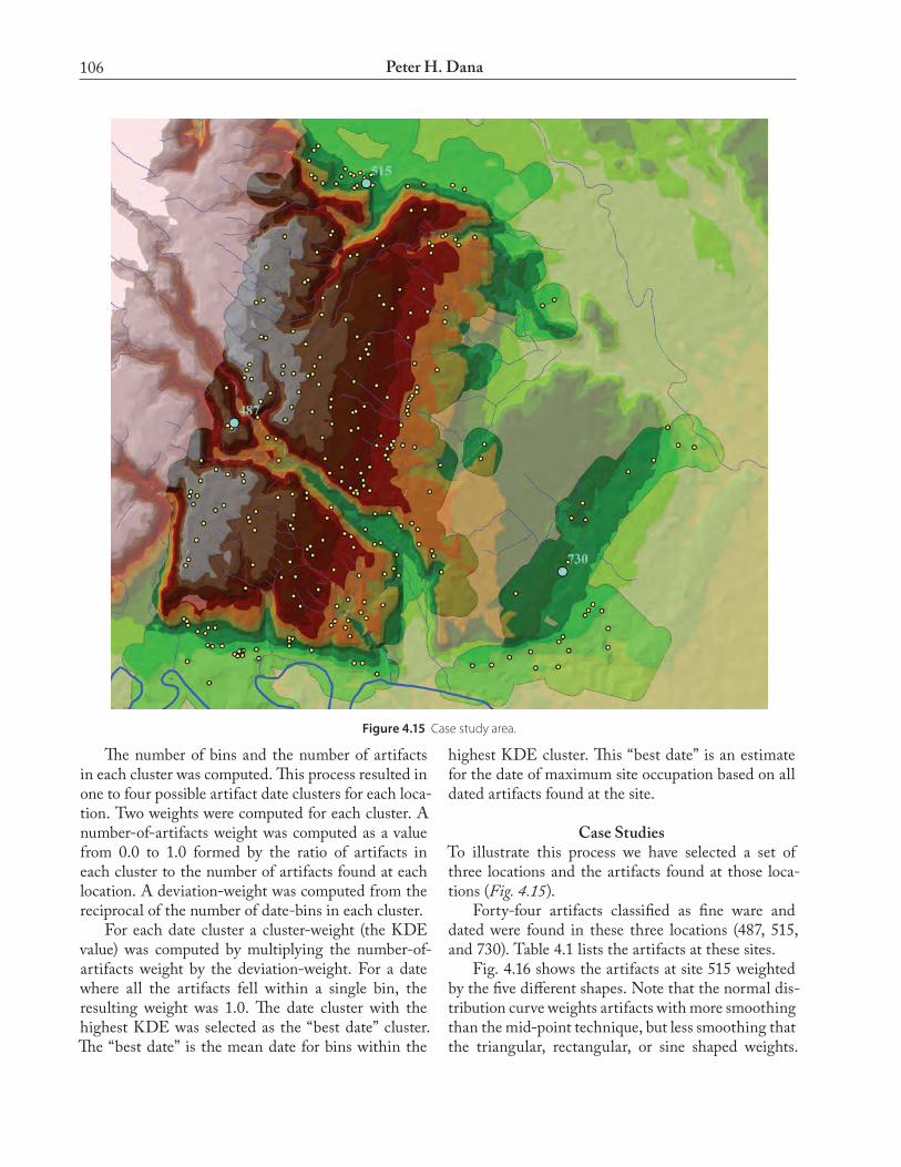
Case StudiesTo illustrate this process we have selected a set of three locations and the artifacts found at those loca-tions (Fig. 4.15). Forty-four artifacts classified as fine ware and dated were found in these three locations (487, 515, and 730). Table 4.1 lists the artifacts at these sites. Fig. 4.16 shows the artifacts at site 515 weighted by the five different shapes. Note that the normal dis-tribution curve weights artifacts with more smoothing than the mid-point technique, but less smoothing that the triangular, rectangular, or sine shaped weights.

Figure 4.15 Case study area.


LOC_ID Form Function Part Type ILL Beg. date End date

487 sk Drinking Sh PSk3b cf. 622-01 550 480

487 sk Drinking R C-S20/28 cf. 043-08 320 280


487 CC Food Serv F CC2 cf. 521-07 420 300

487 C Drinking RSh IC5b cf. 622-02 600 550

515 sk Drinking F ionic cf. 395-19 480 440

515 sk Drinking F C-S25/S33 cf. 523-23 440 400

515 SA Food Serv B SA3a cf. 260-24 350 270

515 C Drinking RSh IC4 cf. 397-47 580 540

515 C Drinking Sh IC6 cf. 477-43 460 430

515 C Drinking R CO6c cf. 454-06 350 250

515 C Drinking FB B6 515-03 200 100

515 C Drinking FB cf. GW_372 200 100

515 B Food Serv R B1 cf. 501-17 300 200

730 large ves Drinking R 730-17 320 300

730 sk Drinking F C-S33/S49 cf. 521-11 410 375

730 sk Drinking F A-S71 cf. 241-07 400 350

730 sk Drinking B ? NO 400 300


730 sk Drinking RH C-S20/28 cf. 521-54 320 280





730 sk Drinking RH C-S20/28 cf. 395-05 320 280

730 sk Drinking R C-S65 cf. 454-08 320 280

730 SB Food Serv R SB6 cf. 354-03 320 250



730 op? ? R NO 400 350

730 op ? F NO 430 350

730 op ? B rb 425 300

730 op ? B rb 400 300

730 op ? F NO 350 300

730 op ? R NO 350 250

730 op ? B rb 325 250

730 Kr? Drinking R NO 450 350

730 Dish Food Serv F D22 cf. 501-16 310 150

730 CC Food Serv R CC1-rb cf. 521-03 400 300

730 C Drinking FB stl cf. 428-01 410 300


730 C Drinking F IC4-5 cf. 397-53 600 550

Table 4.1 Case study site artifacts.

108 Peter H. Dana

Figure 4.16 Location 515 artifacts and “best dates.”


Code Type

GFW Glazed Fine Ware

FFW Fig.d Fine Ware

TWC Coarse Table Ware

COW Cooking Ware

STW Storage Wares

LMW Loom Weights

TCF Terracotta Figurines

TOT Tomb Tiles

Table 4.2 Code definitions.

The normal distribution curve shape tends to be sensi-tive to changes in artifact weights over the range of dates, while not smoothing so much that rises and dips in “occupation” are ignored. The normal curve shape seems to allow the “best date” algorithm to pick out the date of most probable maximum occupation with considerable sensitivity.

Site TypingIn addition to site dating, we attempted to use sta-tistical methods to identify clusters of correlated ratio patterns in all types of ceramics found at sites. We searched for ratio patterns that might represent meaningful signatures of location types such as farm-houses, tombs, or other kinds of sites. We produced a list of survey locations (sites and plots) with counts of artifacts distributed in eight categories (Table 4.2) considered to provide the most discrimination be-tween different types of sites. Correlations between one set of ratios (or artifact counts) and another were determined by computing a simple correlation coefficient from two sets of ratios or counts. The procedure works with ratios or counts in any combination because the correlation coefficient is identical for all cases. As long as the order of the categories is the same for both ratio (or count) sets, the procedure results in the same coefficient. The correlation coefficient, r, is computed from two sets of ratios or counts consisting of pairs of X and Y values:

r = Sum XY / (Sqrt(Sum X^2) * Sqrt(Sum(Y^2)5

The range of r is -1 to +1, with -1 values suggesting negative correlation, zero values indicating no cor-relation, and +1 values suggesting positive correlation. To evaluate r for different numbers of categories, we 5 J.C. Davis 1986, 40, No. 2.24.

computed a t-distribution value from r and the de-grees of freedom. Eight categories yield 6 degrees of freedom (df).

t = r * Sqrt(df) / Sqrt(1-r^2)6

For a 95% probability that X and Y are correlated in eight categories, the critical value for t (CTV) is 2.447. For a 99% significance level, the CTV is 3.707.7 The method is a variation and subset of unsuper-vised classification using the chain method.8 It finds a mean set of category ratios from the best matches to the composite ratio as it passes through the database of ratios or counts of artifacts in each category. The method picks the same clusters and same mean ratios from data sets sorted in arbitrary orders.

Location Artifact Category CorrelationWe computed the correlation coefficients between categories for all locations to see if any categories were so highly correlated with each other that their mutual inclusion was redundant (Table 4.3).

Method DetailsThe method was implemented with a MatLab script. The program flow is illustrated by the following pseudo-code:Set critical t-distribution value for level of significance of correlation LoopPass One: Find mean pattern of all unused locationsPass Two: Find location that is best match to that mean (best match is highest correlation coefficient). Mark that location as used. That location is the start of a group. The pattern for that location is the start for a group signature. Loop to populate a group.

Locations are added to the group (and marked as used) if they are the next best match and their t-scores are over the critical t-value for the level of significance.

The patterns for added locations are incorporated into the composite signature.

6 J.C. Davis 1986, 67, No. 2.35.7 J.C. Davis 1986, 62.8 Jensen 1986, 231–34.

110 Peter H. Dana

GFW FFW TWC COW STW LMW TCF TOT

GFW 1.000 0.217 0.779 0.797 0.636 0.306 0.330 0.027

FFW 0.217 1.000 0.114 0.073 0.133 0.045 0.018 0.182

TWC 0.779 0.114 1.000 0.795 0.620 0.323 0.199 -0.010

COW 0.797 0.073 0.795 1.000 0.646 0.301 0.226 -0.018

STW 0.636 0.133 0.620 0.646 1.000 0.289 0.138 0.083

LMW 0.306 0.045 0.323 0.301 0.289 1.000 0.128 -0.018

TCF 0.330 0.018 0.199 0.226 0.138 0.128 1.000 -0.017

TOT 0.027 0.182 -0.010 -0.018 0.083 -0.018 -0.017 1.000

Table 4.3 Cross correlation between categories (see Table 4.2 for code defintions).

When no more unused locations fit the t-criteria the group is complete.

The composite signature is added to the list of signatures.Pass Three: Each location is matched to the signature that it best matches.Pass Four Locations in each group are used to form a composite signature

Five files are produced:wareclusters.wk1 is a list of groups and the locations

used in the formation of those groups’ signatures.

waregroups.wk1 is a list of locations and the group they best match.

waresignatures.wk1 is a list of the group signatures.groupclusters.wk1 is a list of the groups, the number

in each group and the locations within each group.

groupsignatures.wk1 is a list of the final signatures for each group.

TestsA sample file was produced as a check of the method’s accuracy. The artificial test locations have a SUM value of =INT(RAND()*100)+11. The patterns use that SUM value and the following multipliers to compute artifact

Pattern GFW FFW TWC COW STW LMW TCF TOT Sum

P1 3 1 4 1 5 9 2 6 31.000

P2 6 2 9 5 1 4 1 3 31.000

P3 5 9 2 6 3 1 4 1 31.000

P4 1 4 1 3 6 2 9 5 31.000

P5 4 4 4 4 4 4 4 3 31.000

P6 1 1 2 3 4 5 6 9 31.000

P7 8 0 12 6 5 0 0 0 31.000

P8 14 4 9 2 2 0 0 0 31.000

Table 4.4 Patterns in random location artifact counts (see Table 4.2 for code defintions).

Pattern p1 p2 p3 p4 p5 p6 p7 p8

P1 1.000 0.035 -0.835 -0.191 -0.312 0.489 -0.193 -0.267

P2 0.035 1.000 -0.191 -0.835 0.129 -0.418 0.799 0.663

P3 -0.835 -0.191 1.000 0.035 0.423 -0.645 -0.058 0.224

P4 -0.191 -0.835 0.035 1.000 -0.165 0.546 -0.588 -0.645

P5 -0.312 0.129 0.423 -0.165 1.000 -0.753 0.340 0.308

P6 0.489 -0.418 -0.645 0.546 -0.753 1.000 -0.565 -0.717

P7 -0.193 0.799 -0.058 -0.588 0.340 -0.565 1.000 0.743

P8 -0.267 0.663 0.224 -0.645 0.308 -0.717 0.743 1.000

Table 4.5 Cross correlations for patterns.


counts in each category =INT(SUM/8*(RAND()*M)) with the following multipliers (M): Patterns P1-4 and P6 are variations on the digits 31415926. Pattern P5 is a 44444443 pattern representing almost equal values in each category. Pattern P7 is based on a hypothetical farmhouse sig-nature composited from four excavated farmhouses (Sant’Angelo Grieco, San Biagio, Fattoria Stefan, and Fattoria Fabrizio). Pattern P8 is based on a hypotheti-cal composite tomb/necropolis signature derived from the Pantanello necropolis burials (Tables 4.4 and 4.5). Larger cross correlations (r>.50) exist for P4 and P6, P2 and P7, P2 and P8, and for P7 and P8. This suggests that the farmhouse (P7) and tomb (P8) sig-natures are similar and that P2 is similar to both the tomb/necropolis and the farmhouse. The expected ratio signatures from these groups are shown in Table 4.6. The script was run with a CTV of 5.208 (99.9%) on the test data. The algorithm grouped the test loca-tion patterns into the clusters shown in Table 4.7. The signatures for each group are shown in Table 4.8. Pattern P5 was distributed into 91 different groups with 91 unique signatures.

Signature Analysis of All Location Artifact Counts

The script was run using the list of 912 locations and their artifact counts. 43 signatures resulted (Table 4.9). Of these, 15 were associated with ten or more locations. The detected signatures have correlation coef-ficients with respect to the composite farmhouse and tomb signatures; these are converted to t-values. The groups in bold in Table 4.10 show the detected signatures that correspond to farmhouse and tomb/necropolis signatures with a CTV of more than 5.207 for a 99.9% significance. This suggests that signatures 1 and 4 match a farm-house and that signature 3 matches a tomb/necropolis. Note that signature 1 is very close to matching both a farmhouse and a tomb/necropolis, reflecting the strong cross correlation between the two site-types. Approximately one-third (332) of the locations were classified as farmhouses (in two categories) or tombs/necropoleis. The others were unclassified at this (99.9%) level of significance. We ran similar cluster analysis tests using the Two-Step and K-Means processes in SPSS. Similar signatures resulted, but with differences in the assign-ment of locations to detected signatures.

GFW FFW TWC COW STW LMW TCF TOT

P1 0.097 0.032 0.129 0.032 0.161 0.290 0.065 0.194

P2 0.194 0.065 0.290 0.161 0.032 0.129 0.032 0.097

P3 0.161 0.290 0.065 0.194 0.097 0.032 0.129 0.032

P4 0.032 0.129 0.032 0.097 0.194 0.065 0.290 0.161

P5 0.129 0.129 0.129 0.129 0.129 0.129 0.129 0.097

P6 0.032 0.032 0.065 0.097 0.129 0.161 0.194 0.290

P7 0.258 0.000 0.387 0.194 0.161 0.000 0.000 0.000

P8 0.452 0.129 0.290 0.065 0.065 0.000 0.000 0.000

Table 4.6 Expected signatures from test patterns.

Group Pattern Total Included Excluded Mis_Cat

G1 P7 100 100 0 0

G2 P8 100 100 0 0

G3 P6 100 100 0 0

G37 P2 100 100 0 0

G38 P4 100 100 0 0

G46 P3 100 100 0 0

G47 P1 100 100 0 0

Table 4.7 Detected clusters from algorithm on test data.

112 Peter H. Dana

Pattern GFW FFW TWC COW STW LMW TCF TOT

P1 0.097 0.032 0.129 0.032 0.161 0.290 0.065 0.194

G47 0.094 0.029 0.130 0.031 0.163 0.299 0.062 0.192

P2 0.194 0.065 0.290 0.161 0.032 0.129 0.032 0.097

G37 0.195 0.063 0.294 0.164 0.027 0.131 0.030 0.096

P3 0.161 0.290 0.065 0.194 0.097 0.032 0.129 0.032

G46 0.161 0.295 0.059 0.191 0.097 0.032 0.133 0.031

P4 0.032 0.129 0.032 0.097 0.194 0.065 0.290 0.161

G38 0.033 0.125 0.034 0.093 0.196 0.056 0.305 0.158

P5 0.129 0.129 0.129 0.129 0.129 0.129 0.129 0.097

P6 0.032 0.032 0.065 0.097 0.129 0.161 0.194 0.290

G3 0.031 0.028 0.065 0.095 0.130 0.160 0.195 0.296

P7 0.258 0.000 0.387 0.194 0.161 0.000 0.000 0.000

G1 0.241 0.014 0.369 0.180 0.152 0.015 0.015 0.016

P8 0.452 0.129 0.290 0.065 0.065 0.000 0.000 0.000

G2 0.440 0.123 0.284 0.056 0.057 0.015 0.013 0.012

Table 4.8 Expected and detected signatures from random artifact counts.

Group GFW FFW TWC COW STW LMW TCF TOT

1 0.377 0.005 0.469 0.092 0.047 0.004 0.004 0.001

2 0.117 0.002 0.765 0.064 0.047 0.004 0.002 0.000

3 0.572 0.008 0.265 0.086 0.052 0.004 0.010 0.003

4 0.249 0.000 0.309 0.162 0.278 0.000 0.003 0.000

5 0.318 0.000 0.338 0.295 0.041 0.004 0.003 0.001

6 0.134 0.005 0.495 0.075 0.277 0.012 0.002 0.000

7 0.578 0.000 0.047 0.037 0.336 0.000 0.002 0.000

9 0.380 0.008 0.339 0.017 0.247 0.007 0.000 0.001

10 0.113 0.000 0.456 0.226 0.190 0.014 0.000 0.000

13 0.028 0.008 0.456 0.479 0.030 0.000 0.000 0.000

14 0.092 0.000 0.021 0.004 0.875 0.008 0.000 0.000

15 0.454 0.000 0.130 0.391 0.025 0.000 0.000 0.000

17 0.935 0.010 0.017 0.014 0.021 0.000 0.000 0.003

21 0.107 0.005 0.591 0.288 0.007 0.002 0.000 0.000

29 0.047 0.000 0.423 0.004 0.526 0.000 0.000 0.000

Table 4.9 Signatures detected by algorithm from location data.

error Analysis and Quality Control The estimated spatial resolution for each of the layers used in the farm distribution analysis is pre-sented in Table 4.11. Based on these spatial resolutions, we can expect 32 m of meaningful spatial resolution for analysis that excludes the geomorphology layer and the DEM, 54 m excluding the DEM alone, and 116 m if all layers are used.

Date-bins have a quantization size of fifty years, so we expect date analysis to be meaningful at the 100-year level.

Division Line AnalysisThere are two distinct sets of division lines; those north, and those south of the Basento. The division lines in each set are mostly aligned along one direction. This analysis does not consider the “transverse” division


lines, only those aligned in the principle direction within each set. We focus here on the northern set of lines within the study area north of the Basento.

Proximity of Farms to Division LinesWe attempted to answer the question of whether or not farm sites were near to division lines. We began with a subset of division lines, those within the study area aligned along the primary division line axis. We constructed a set of extended division lines, connecting line segments that were aligned. With a layer containing all sites identified as farms, we performed a spatial join, resulting in a table of perpendicular distances between each farm and the nearest division line. The resulting distribu-tion is multi-modal, with peak at about 35 and 45 m and others at 75 and 95 m (Fig. 4.17). A chi-square test for independence was per-formed that suggested that for 20-m histogram bins

the observed distribution had a 12.9% probability of occurring by chance (Fig. 4.18).

necropoleis and Division LinesWe attempted to answer the question of whether or not necropoleis were near to division lines. We began with a subset of extended division lines, those within the study area aligned along the primary division line axis. With a layer containing all sites identified as necropoleis, we performed a spatial join, resulting in a table of perpendicular distances between each necropolis and the nearest division line. We then selected those 75 necropoleis within 120 m (about half the distance between parallel division lines) of a divi-sion line. The resulting distribution is bi-modal, with a peak at about 5 m and another at 60 m (Fig. 4.19). Fifty necropoleis are within 60 m of a division line and twenty-five between 60 and 120 m from the nearest line. A chi-square test for independence was

Group Count r FH r Tomb t- FH T - Tomb

1 228 0.919 0.898 5.708 5.000

2 290 0.835 0.548 3.715 1.607

3 91 0.703 0.951 2.423 7.503

4 12 0.924 0.678 5.932 2.258

5 32 0.899 0.780 5.029 3.055

6 29 0.884 0.526 4.634 1.517

7 14 0.436 0.685 1.186 2.301

9 12 0.845 0.851 3.870 3.974

10 17 0.931 0.495 6.230 1.396

13 16 0.710 0.266 2.469 0.675

14 15 0.145 -0.065 0.359 -0.159

15 10 0.588 0.678 1.779 2.258

17 42 0.354 0.795 0.928 3.205

21 23 0.860 0.505 4.135 1.433

29 12 0.613 0.225 1.902 0.566

Table 4.10 Detected signatures and correlation with farmhouse and tomb signatures.

Table 4.11 Spatial resolution of layers.

Layer Spatial resolution (m) Source

Site positions 10 GPS or 1:10,000 maps

Survey plots 10 GPS or 1:10,0000 maps

Site elevations 2.5 5 meter elevation contours

Streams 20 Polylines from 1:10,000 maps

Division lines 20 Georegistered aerial photographs

Geomorphology 50 Digitized from aerial photographs

DEM 100 Radar DEM

114 Peter H. Dana

Figure 4.17 Distance from farms to division lines.

Figure 4.18 Significance of distance distribution (farms to division lines).

Figure 4.19 Distance from necropoleis to division lines.

Figure 4.20 Significance of distance distribution (necropoleis to division lines).


performed that suggested that for 20-m histogram bins the observed distribution had a 1.3% probability of occurring by chance (Fig. 4.20).

Division Line Azimuths and SlopesNext we investigated the directions and slopes of the division lines with respect to the terrain surface. This analysis is highly speculative because we only have modern terrain surfaces to work with and our knowledge of those surfaces is derived from aerial photographs used to make topographic maps or digi-tal elevation models derived from modern satellite imagery. Division lines were extracted from the original data set resulting in South and North division line geodatabase feature classes projected in PTM co-ordinates. These contained only those division lines parallel to the primary axes for each region. First we established the directions of the divi-sion lines with respect to true north. Azimuths are angles between 0 and 360° measured clockwise from true north. To avoid the convergence angle errors as-sociated with some map projections we performed all this analysis in the Pantanello Transverse Mercator (PTM) coordinate system described above. This analysis of division line slopes and azimuths and terrain is based on two digital elevation models: A

NASA Advanced Spaceborne Thermal Emission and Reflection Radiometer (ASTER) DEM and a NASA Shuttle Radar Topography Mission (SRTM) DEM. The SRTM DEM in the 3 arc second finished format was downloaded from the USGS Seamless server in June of 2009. The ASTER Global Digital Elevation Model (GDEM) was downloaded from NASA’s EOS data archive in July of 2009. Both original DEM tiles were projected into the PTM coordinate system. These two DEMs come from different sources and methods. The ASTER DEM has cell sizes of about 27 m and the SRTM cell size is about 80 m. Over the region containing division lines they are very similar in their elevation values. The SRTM mean value is about 5 m higher than the ASTER mean. As digitized from the original aerial photographs, projected with the PTM system, and measured using the COGO functions of ArcGIS, the northern set of lines in the principal direction have a mean azimuth of 131.0° (or a back azimuth of 311.0°). The standard de-viation of azimuth is 1.0°. For the southern set of lines the principle axis azimuth is 108.5° (back azimuth 288.5°) with a standard deviation of 1.1°. The two sets of lines then are very much parallel lines within each set, but the mean azimuths of the two sets differ by 22.5°. One of the enduring division line mysteries is this considerable difference in the primary direction of these two sets of parallel lines. Fig. 4.21 shows the orientation of the north and south division lines. Note that the southern set of lines is close to perpendicular to the contour lines while the northern set point at an oblique angle to the contour lines. A line perpendicular to a contour line describes a direction that is the aspect of the terrain at the point of intersection. In trying to make some sense of this we attempted to see what the relationship of the division line azi-muths was to the aspects of the two terrain surfaces on which they lie. The aspect of a terrain surface is the direction that a downhill line faces. Of course for almost any real surface this idea is not so simple. Downhill paths often follow complex paths and so the aspect of a surface is also complex. It is difficult to find the average of cyclical attri-butes such as direction. Simple averaging fails because simple averaging does not take into account the wrap-ping of azimuths between 360 and 0°. For example, a northwestern azimuth of 340° and a northeastern

Figure 4.21 Division lines and elevation contours.

116 Peter H. Dana

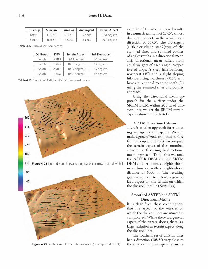
azimuth of 15° when averaged results in a numeric azimuth of 177.5°, almost due south rather than the actual mean direction of 357.5°. The arctangent (a four-quadrant atan2(x,y)) of the summed sines and summed cosines of angles results in a directional mean. This directional mean suffers from equal weights of each angle irrespec-tive of slope. A steep hillside facing northeast (45°) and a slight sloping hillside facing northwest (315°) will have a directional mean of north (0°) using the summed sines and cosines approach. Using the directional mean ap-proach for the surface under the SRTM DEM within 200 m of divi-sion lines we get the SRTM terrain aspects shown in Table 4.12.

SRTMDirectionalMeansThere is another approach for estimat-ing average terrain aspects. We can make a generalized, smoothed surface from a complex one and then compute the terrain aspect of the smoothed elevation surface using the directional mean approach. To do this we took the ASTER DEM and the SRTM DEM and performed a neighborhood mean function with a neighborhood distance of 1000 m. The resulting grids were used to extract a general-ized aspect for the terrain on which the division lines lie (Table 4.13).

Smoothed ASTeR and SRTM Directional Means

It is clear from these computations that the aspect of the terraces on which the division lines are situated is complicated. While there is a general aspect of the terrace slopes, there is a large variation in terrain aspect along the division lines. The southern set of division lines has a direction (108.5°) very close to the southern terrain aspect estimates

DL Group Sum Sin Sum Cos Arctangent Terrain Aspect

North 1282.68 -411.67 -72.206 107.8 degrees

South 1648.57 -829.85 -63.280 116.7 degrees

DL Group DEM Terrain Aspect Std. Deviation

North ASTER 97.8 degrees 60 degrees

North SRTM 100.9 degrees 55 degrees

South ASTER 108.9 degrees 55 degrees

South SRTM 104.8 degrees 62 degrees

Table 4.13 Smoothed ASTER and SRTM directional means.

Table 4.12 SRTM directional means.

Figure 4.23 South division lines and terrain aspect (arrows point downhill).

Figure 4.22 North division lines and terrain aspect (arrows point downhill).


(104.8 to 116.7°), while the northern division lines have a direction (131.0°) that is oblique to the north-ern terrain aspect estimates (97.8 to 107.8°). Figs. 4.22 and 4.23 show the complex relationship between terrain space and slope. The arrows show terrain aspect, their length indicating slope (longer = steeper). It is clear that the northern division lines have a pronounced angle oblique to the terrain aspect. The southern lines are much closer to the terrain aspect angle. Next we looked at the slopes of division lines with respect to the terrain slopes. Fig. 4.24 shows the angle

of the smoothed terrain over the north and south re-gions in degrees. In both regions where we find division lines the ter-rain slopes are gentle and generally less than 2.0° (3.5%). For the ASTER and SRTM DEMs, the terrain slopes (measured downhill) within 200 m of the divi-sion lines are shown in Table 4.14. Golden Software’s Surfer platform was used to com-pute the slope of each division line by producing a terrain

“slice” along each division line. The slices contain X, Y, distance, and elevation for each intersection between the DEM cells and the lines. Using the distance and eleva-tions a linear regression function was used in Excel to

Figure 4.24 Slopes of the smoothed terrain.

DL Group DEM Slope Degrees Slope Percent

North ASTER -0.8223 -1.44

North SRTM -0.9146 -1.59

South ASTER -0.9443 -1.64

South SRTM -0.9905 -1.72

Table 4.14 Terrain slopes within 200 m of division lines.

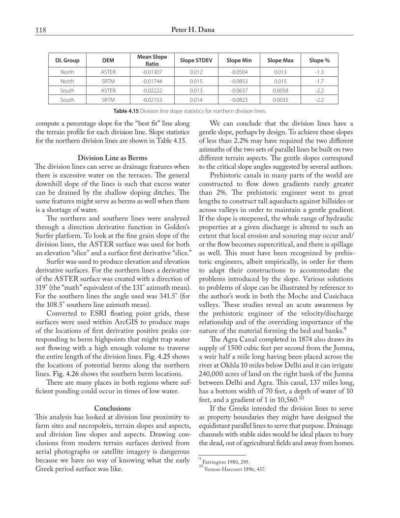
118 Peter H. Dana

compute a percentage slope for the “best fit” line along the terrain profile for each division line. Slope statistics for the northern division lines are shown in Table 4.15.

Division Line as BermsThe division lines can serve as drainage features when there is excessive water on the terraces. The general downhill slope of the lines is such that excess water can be drained by the shallow sloping ditches. The same features might serve as berms as well when there is a shortage of water. The northern and southern lines were analyzed through a direction derivative function in Golden’s Surfer platform. To look at the fine grain slope of the division lines, the ASTER surface was used for both an elevation “slice” and a surface first derivative “slice.” Surfer was used to produce elevation and elevation derivative surfaces. For the northern lines a derivative of the ASTER surface was created with a direction of 319° (the “math” equivalent of the 131° azimuth mean). For the southern lines the angle used was 341.5° (for the 108.5° southern line azimuth mean). Converted to ESRI floating point grids, these surfaces were used within ArcGIS to produce maps of the locations of first derivative positive peaks cor-responding to berm highpoints that might trap water not flowing with a high enough volume to traverse the entire length of the division lines. Fig. 4.25 shows the locations of potential berms along the northern lines. Fig. 4.26 shows the southern berm locations. There are many places in both regions where suf-ficient ponding could occur in times of low water.

ConclusionsThis analysis has looked at division line proximity to farm sites and necropoleis, terrain slopes and aspects, and division line slopes and aspects. Drawing con-clusions from modern terrain surfaces derived from aerial photographs or satellite imagery is dangerous because we have no way of knowing what the early Greek period surface was like.

We can conclude that the division lines have a gentle slope, perhaps by design. To achieve these slopes of less than 2.2% may have required the two different azimuths of the two sets of parallel lines be built on two different terrain aspects. The gentle slopes correspond to the critical slope angles suggested by several authors. Prehistoric canals in many parts of the world are constructed to flow down gradients rarely greater than 2%. The prehistoric engineer went to great lengths to construct tall aqueducts against hillsides or across valleys in order to maintain a gentle gradient. If the slope is steepened, the whole range of hydraulic properties at a given discharge is altered to such an extent that local erosion and scouring may occur and/or the flow becomes supercritical, and there is spillage as well. This must have been recognized by prehis-toric engineers, albeit empirically, in order for them to adapt their constructions to accommodate the problems introduced by the slope. Various solutions to problems of slope can be illustrated by reference to the author’s work in both the Moche and Cusichaca valleys. These studies reveal an acute awareness by the prehistoric engineer of the velocity/discharge relationship and of the overriding importance of the nature of the material forming the bed and banks.9 The Agra Canal completed in 1874 also draws its supply of 1500 cubic feet per second from the Jumna, a weir half a mile long having been placed across the river at Okhla 10 miles below Delhi and it can irrigate 240,000 acres of land on the right bank of the Jumna between Delhi and Agra. This canal, 137 miles long, has a bottom width of 70 feet, a depth of water of 10 feet, and a gradient of 1 in 10,560.10

If the Greeks intended the division lines to serve as property boundaries they might have designed the equidistant parallel lines to serve that purpose. Drainage channels with stable sides would be ideal places to bury the dead, out of agricultural fields and away from homes.

9 Farrington 1980, 295.

10 Vernon-Harcourt 1896, 437.

DL Group DEM Mean Slope Ratio Slope STDEV Slope Min Slope Max Slope %

North ASTER -0.01307 0.012 -0.0504 0.013 -1.3

North SRTM -0.01744 0.015 -0.0853 0.015 -1.7

South ASTER -0.02222 0.013 -0.0637 0.0058 -2.2

South SRTM -0.02153 0.014 -0.0823 0.0035 -2.2

Table 4.15 Division line slope statistics for northern division lines.


Figure 4.25 Locations of ponding berms along northern lines.

Figure 4.26 Locations of ponding berms along southern lines.

120 Peter H. Dana

If they intended the lines to serve as drainage features in times of excess water they might have selected these critical slope angles that allow for runoff without chan-nel scouring while keeping the channels clear of silt. If their intention was to retain water in times of drought, the ponding areas behind the berms along the lines might have been advantageous. Any conclusions must remain speculative without some way of reconstructing the terrain when the lines were constructed.

Farm Site DistributionsWe have based our analysis of farm site distributions and farm importance on sites identified as farms by field investigators, rather than by the statistical meth-ods explained above, because the on-site observations offer a more complete interpretive picture. We employed the idea of Multiple Criteria Evalu-ation (MCE), based on a weighted linear combination of expert opinions, subjective judgments, quantitative measurements, and fuzzy estimation. The basis of this analysis is a layer of farm sites that could be dated by fine-ware artifacts. The layer consists of sites and survey plot centroids described as definite farmhouses, probable farmhouses, and combination farmhouse/tomb sites. Attributes used include best date, date histograms, scatter area, density of tile frag-ments, and density of all other ceramic artifacts.

Farm Significance and Distribution for each Location for All Date Periods

The estimate of farm size or importance is based on the size of the scatter, ceramic density, tile density, number of dated fine-ware artifacts, and the size of scatters in each best date period.

We calculated weights for these fields based on the following fuzzy sets for density (tile and ceramic): Very Heavy = 9 Heavy = 7 Moderate = 5 Light = 3 No Data = 0 <Null> = 0The approximate scatter size (length x width) for all locations was reclassified into values from 1 to 9. The distribution of scatter sizes from 0 to 5000 is almost linear; above 5000 the distribution makes a rapid change to a maximum of 42,000. The threshold for inclusion in category 9 was therefore set to 5000, with the values from 0 to 4999 distributed evenly between 1 and 8.The Area Weight (ARW) =IIF( [AREA_LW] >=5000, 9, IIF ( [AREA_LW] > 0, [AREA_LW] * .0016 +1,0))

The Tile Density Weight (TDW) =IIF( [TILE_DENS]=”Very Heavy”, 9,IIF( [TILE_DENS] =”Heavy”, 7,IIF( [TILE_DENS] =”Moderate”, 5,IIF( [TILE_DENS] =”Light”, 3,IIF( [TILE_DENS] =”None”, 1,0)))))

The Ceramic Density Weight (CDW) =IIF( [CERAM_DENS]=”Very Heavy”, 9,IIF( [CERAM_DENS] =”Heavy”, 7,IIF( [CERAM_DENS] =”Moderate”, 5,IIF( [CERAM_DENS] =”Light”, 3,IIF( [CERAM_DENS] =”No Data”, 0,0)))))]

Farm-Size Weight for each Date PeriodWe computed a maximum weighted-distance (MWD) value for use in a cost-weighted allocation

Best Date Range Number of Sites Mean ARW MWD

250 (275–225) 15 4.2 178

300 (325–275) 92 4.4 184

350 (375–325) 56 3.9 170

400 (425–375) 23 3.6 162

450 (475–425) 21 3.5 158

500 (525–475) 5 3.9 170

550 (575–525) 42 3.2 148

600 (625–575) 2 3.3 152

Table 4.16 Maximum distance weight.


(see below). We selected the farmhouse locations with a best date within the fifty-year period of the date histogram. The MWD value (Table 4.16) is four times the square root of the mean area, or 4* SQT( (Mean ARW-) / 0.016.

Date-Independent Multiple Criteria evaluationfor each Location

A date-independent multiple criteria evaluation (IMCE) value from 0 to 10 was computed for each location based on the following weights (which sum to 1.0) for relative importance of the categories:

ARW= .50 AreaTDW= .25 Tile densityCDW= .25 Ceramic density

We computed the IMCE weight based on tile and ceramic density and scatter size/area. For the five sites where area was not recorded, leaving a value of 0, a value of 1943 was inserted instead, the average area of all farmhouses (except for the two highest values, 42,000 and 22,500). Weights are equally split be-tween ceramic and tile density (50%) and area (50%). The intention of the method is to give area a weight of 1.0 where there are no density values, and to give arti-

fact density a total weight of 0.5 and area a weight of 0.5 where there are both area and tile/ceramic density measurements. Table 4.17 shows the possible cases. The IMCE value is a result of the linear combina-tion of CDW, TDW, and ARW weighted when all are present by TDW * .25 + CDW * .25 + ARW * .5 or when one or more values are not present by the following:( IIF ( [CDW] + [TDW] <1, [ARW], IIF( [ARW] < 1 And ( [CDW] * [TDW] < 1) , [CDW] + [TDW], IIF( [ARW] > 0 And ( [CDW] * [TDW] > 0) , [ARW] * .5 + ( [CDW] + [TDW] ) * .25, [ARW] * .5 + ( [CDW] + [TDW] ) * .5 ))))

This weight is high (10) for farmhouse locations with very heavy tile and ceramic density and large scatter sizes. The value is low (0) for farmhouse loca-tions with light density and small scatter sizes.

Farm Site Locations for each Date PeriodWe formed layers for eight of the twelve date periods based on the date histogram bins. Locations within a date bin were selected where the date bin sum was more than or equal to 0.95, just less than one artifact’s total weight. Table 4.18 shows the date periods and the number of sites estimated to be occupied in that period.

Location Artifact Weight for each Date Period For each location a weight from 0 to 10 was computed for a specific date period based on the ratio of the num-ber of dated artifacts found at that location to the num-ber of artifacts dated within that specific date period.

LAW = Sum of dated artifacts at this location / Sum of all dated artifacts * 10[SUM_Bnnn] / [SUM_NARTS] *10

Case ARW CDW TDW AW CW TW

0 0 0 0 X X X

1 0 0 NZ X X 1

2 0 NZ 0 X 1 X

3 NZ 0 0 1 X X

4 NZ 0 NZ .5 X .5

5 NZ NZ 0 .5 .5 X

6 NZ NZ NZ .5 .25 .25

Table 4.17 Cases for IMCE categories. (NZ = non-zero, X = don’t care).

Date Period Number of Sites

600 23

550 69

500 18

450 79

400 89

350 105

300 143

250 56

Table 4.18 Locations estimated to be occupied in each period.

122 Peter H. Dana

Location Bin Artifact Weight for All Date PeriodsFor each location a weight from 0 to 10 was computed from the ratio of all artifacts within that date period to the number of artifacts at each location (Table 4.19).

BAW = Sum of dated artifacts at this location for this date period / Sum of all dated artifact histo-grams for this date period * 10[SUM_Bnnn] / [n] *10

Location Total Artifact Weight foreach Date Period

For each location a weight from 0 to 10 was computed from the ratio of dated artifacts to the number of all artifacts (dated or not), in the AdjustedCounts.dbf file, in the field ADJSUM.

TAW = Sum of dated artifacts for this date period / Sum of all artifacts found at this location[SUM_Bnnn] / [ADJSUM] *10

Date-Dependent MCe Value foreach Location and each Date Period

A date-dependent MCE value (DMCE) was com-puted for each site. This was based on these notions:

1. A location with many fine-ware artifacts is more significant than a location with fewer fine-ware artifacts.

2. For a particular fifty-year period a location is more significant when the number of fine-ware artifacts dated within that period is high with respect to the number of fine-ware artifacts dated to all periods found at that location.

3. The number of fine-ware artifacts dated to a particular period is further weighted by the number of fine-ware artifacts of that period at all locations.

Weight Criteria Weight

CDW Ceramic Density 0.0625

TDW Tile Density 0.0625

ARW Area 0.1250

LAWRatio of all dated artifacts to each

date bin0.2500

BAWRatio of dated artifacts at this date to

each date bin0.2500

TAW Ratio of all artifacts to each date bin 0.2500

Table 4.20 Weighting for final MCE value.

Date range Histogram sums of dated artifacts

250 187

300 845

350 340

400 275

450 207

500 143

550 280

600 31

Table 4.19 Histogram sums of dated artifacts for each date range

4. The number of fine-ware artifacts dated to a particular period is further modified by the rela-tive number of all artifacts (whether fine-ware or not) found at that location.

The function for the date-dependent MCE value is: DMCE = LAW * .33333 + BAW * .33333 + TAW *.33333

Final MCe Weight for each LocationAfter a period of evaluation we finally settled on the appropriate weighting for the two components of the MCE process, the date-dependent weight (DMCE) and the date-independent weight (IMCE). To keep the date-independent weight based on tile and ceramic density and area from dominating the rela-tive significance region size, we weighted the linear weighted combination so that DMCE accounted for 75% and IMCE for 25% of the final multiple criteria evaluation (FMCE) weight. A final multiple criteria weight (FMCE) was computed for all locations:

FMCE = IMCE * 0.25 + DMCE * 0.75 The resulting value from 0 to 10 is computed from the weighting scheme shown in Table 4.20.

Farm Cost ValueFarm cost (COST) is a value ranging from 0 for a low-cost (large and important) farm site to 1.0 for a high-cost (small and less important) farm site. COST = (10-FMCE) / 10 The COST value is the basis for a weight surface for each date period. The weight surface is used in a cost-weighted allocation, so that a large farmhouse with high density values is a “low-cost” source, claim-ing more grid cells than a small farmhouse site with low tile and ceramic density resulting in “high cost.”


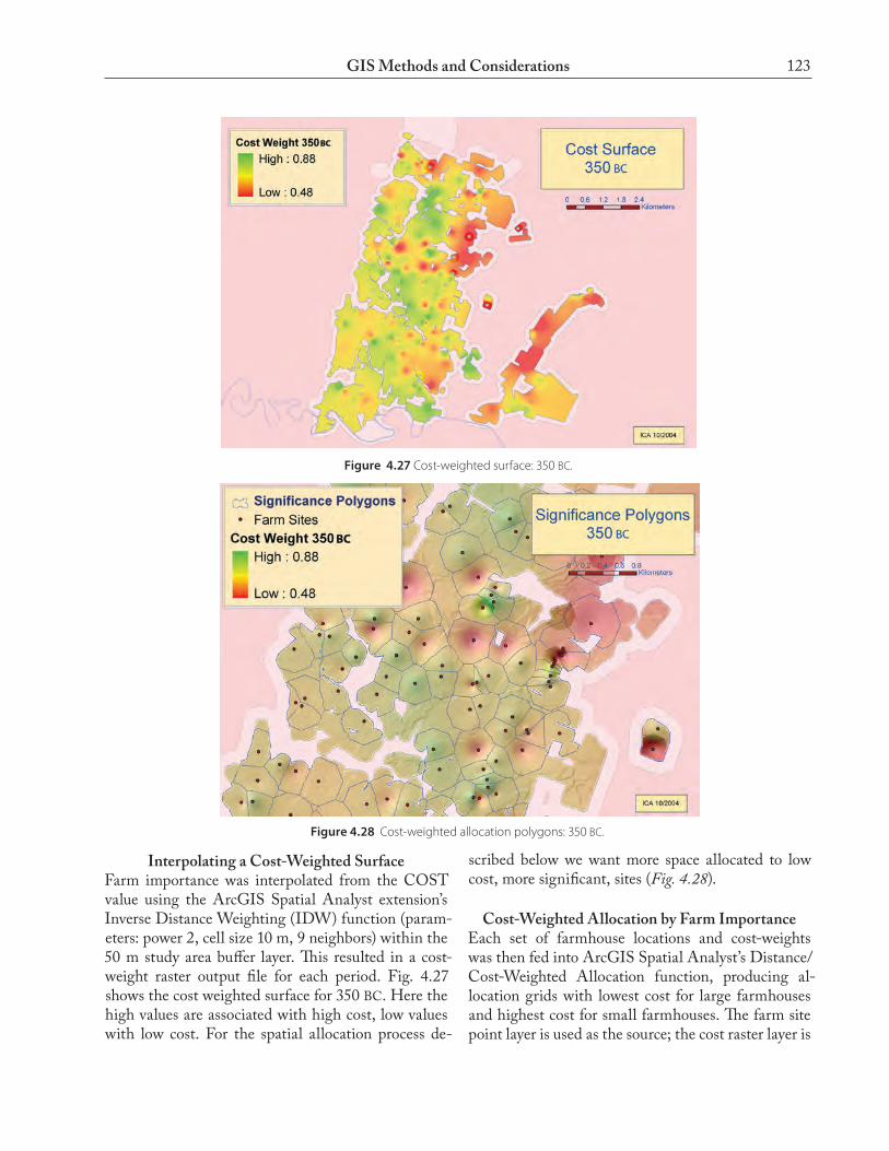
Figure 4.27 Cost-weighted surface: 350 BC.

Figure 4.28 Cost-weighted allocation polygons: 350 BC.

Interpolating a Cost-Weighted SurfaceFarm importance was interpolated from the COST value using the ArcGIS Spatial Analyst extension’s Inverse Distance Weighting (IDW) function (param-eters: power 2, cell size 10 m, 9 neighbors) within the 50 m study area buffer layer. This resulted in a cost-weight raster output file for each period. Fig. 4.27 shows the cost weighted surface for 350 BC. Here the high values are associated with high cost, low values with low cost. For the spatial allocation process de-

scribed below we want more space allocated to low cost, more significant, sites (Fig. 4.28).

Cost-Weighted Allocation by Farm ImportanceEach set of farmhouse locations and cost-weights was then fed into ArcGIS Spatial Analyst’s Distance/Cost-Weighted Allocation function, producing al-location grids with lowest cost for large farmhouses and highest cost for small farmhouses. The farm site point layer is used as the source; the cost raster layer is

124 Peter H. Dana

used as the cost-weighted surface, and the maximum distance is the MWD computed above. The output grids were converted to polygon (vector) features, re-sulting in farm distribution and significance polygon layers. Fig. 4.28 shows the polygons resulting from the cost-weighted allocation process for 350 BC.

Mapping Farm Distribution and SignificanceUsing a gradient fill for the farm polygons, a solid fill for farm site buffers, and small point symbols for farm site centroids, each date period is mapped. Three se-quential date periods are shown in Figs. 4.29–31. A sequence of eight images was used to produce a QuickTime video showing sequential distributions for the periods from 600 to 250 BC (Fig. 4.32). The video allowed researchers to examine change in settlement pattern over time by viewing the entire video or by manually shifting time using the Quick-Time controls.

ConclusionsIn this research GIS was used to assist in the un-derstanding of history by providing a means for

Figure 4.29 Settlement patterns from sinusoidal histograms: 600 BC.

archaeologists to model spatial and temporal dis-tributions through weighted criteria from a variety of archeological evidence. We set up a system with multiple layers and appropriate coordinate systems. We used statistical approaches and multiple criteria evaluation based on the advice of experts. Site types and settlement patterns were considered. Farm sites and the dated artifacts found at them were used to estimate change in space over time. The resulting polygons are not intended to represent the boundaries of farm sites; rather they are the approximate extents of regions of relative spatial significance. They are estimated influence regions, based on weighted evalu-ations of artifacts counts, artifact typology, artifact date ranges, site scatter size and density evaluations, and the weighted opinions of archaeologists. The approach uses an ensemble of sites and arti-facts, not in an attempt to characterize individual sites, but to estimate settlement pattern change over time. The resulting patterns of change within the Metapon-to chora over time and space are intended to provide insights into history through further interpretation by historians, classicists, and archaeologists.

126 Peter H. Dana

Figure 4.32 Video frames, 600 to 250 BC.

4 gis methods and considerations - pdana.com · rome as computed in longitude/latitude space and in...

Documents