4. Lecture

Image enhancement: Filtering

1

• Aims:

– Improvement of image data

– Suppress unwanted distortions

– Highlight interesting features

• Image preprocessing does not increase the

information content

• Best preprocessing is no preprocessing

– better: high quality image acquisition

Image preprocessing

2

Classification of preprocessing

• Point operations – Grayvalue transformations

• Local operations – Spatial filters, look at local

neighbourhoods

• Global operations – Inverse filtering

• Geometric Transformations

3

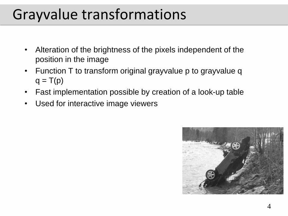
Grayvalue transformations

• Alteration of the brightness of the pixels independent of the

position in the image

• Function T to transform original grayvalue p to grayvalue q

q = T(p)

• Fast implementation possible by creation of a look-up table

• Used for interactive image viewers

4

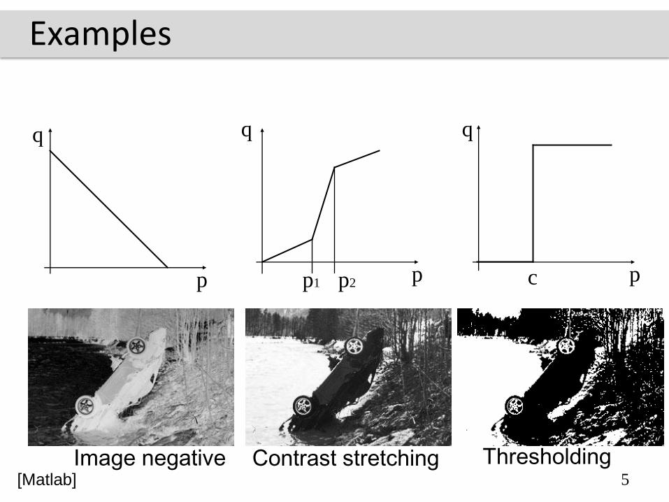
Examples

p

q

p1 p2 c

Image negative Contrast stretching Thresholding

q

p

q

p

5[Matlab]

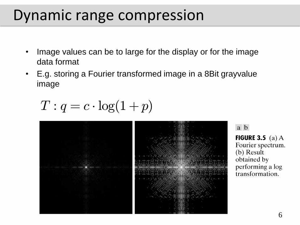
• Image values can be to large for the display or for the image

data format

• E.g. storing a Fourier transformed image in a 8Bit grayvalue

image

T : q = c ¢ log(1+ p)

Dynamic range compression

6

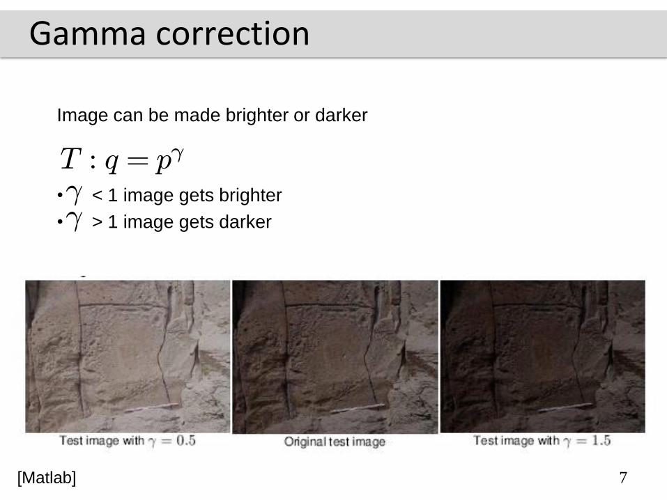
Image can be made brighter or darker

• < 1 image gets brighter

• > 1 image gets darker

Gamma correction

T : q = p°

°°

7[Matlab]

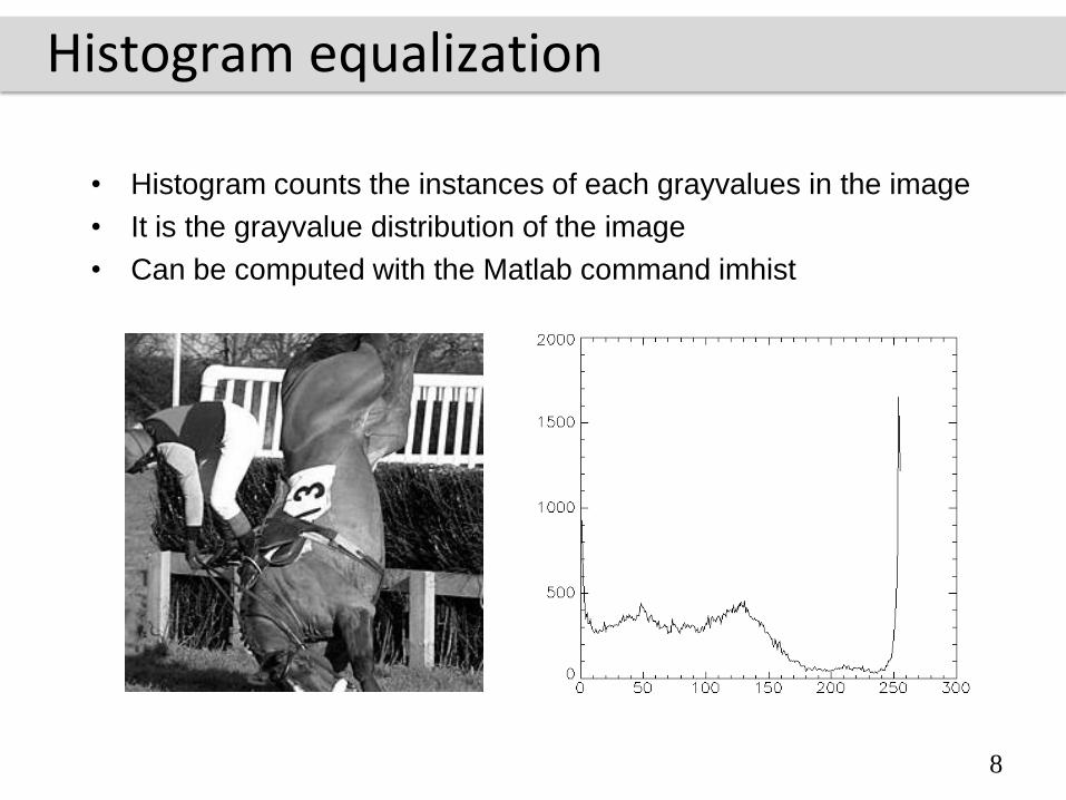
Histogram equalization

• Histogram counts the instances of each grayvalues in the image

• It is the grayvalue distribution of the image

• Can be computed with the Matlab command imhist

8

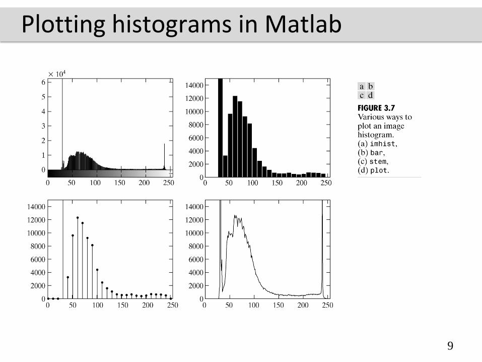
Plotting histograms in Matlab

9

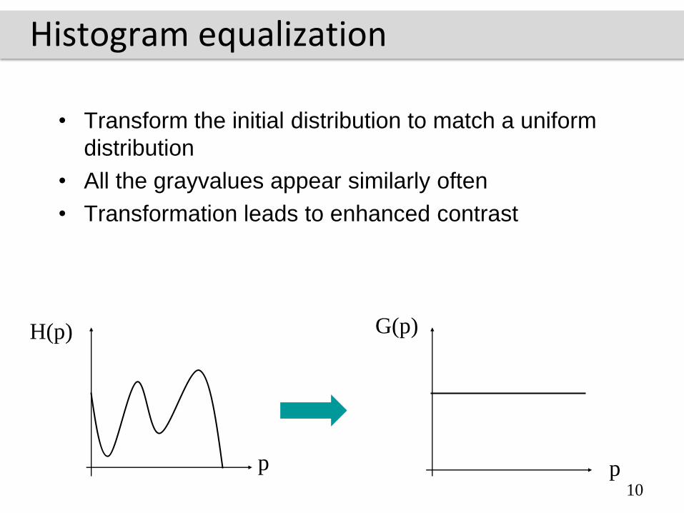
Histogram equalization

• Transform the initial distribution to match a uniform

distribution

• All the grayvalues appear similarly often

• Transformation leads to enhanced contrast

H(p)

p

G(p)

p10

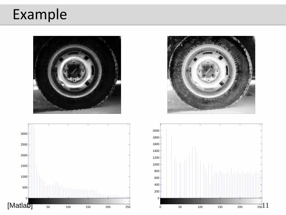
Example

11

0

500

1000

1500

2000

2500

3000

0 50 100 150 200 250

0

200

400

600

800

1000

1200

1400

1600

1800

2000

0 50 100 150 200 250[Matlab]

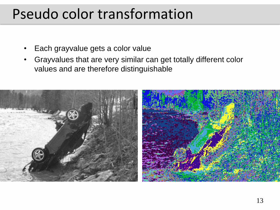
Pseudo color transformation

• Each grayvalue gets a color value

• Grayvalues that are very similar can get totally different color

values and are therefore distinguishable

13

Illumination correction

• When is this necessary?

• Ideally the sensitivity of an image sensor is

independent of the pixel location. This is however not

always true.

• Artificial lighting might lead to non uniform

illumination

• If the deviation is systematic it can be corrected

14

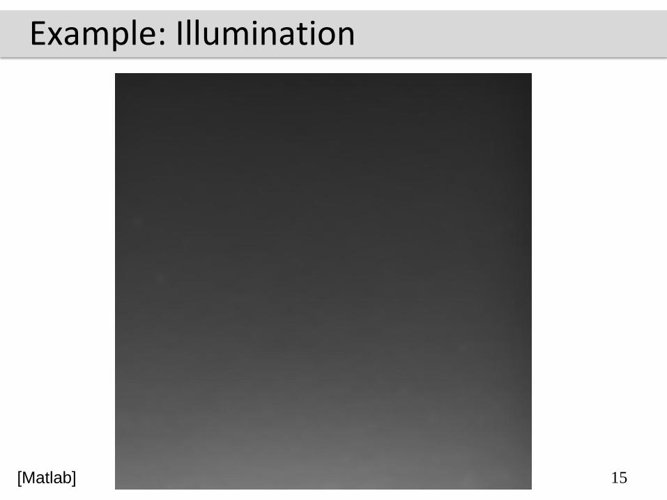
Example: Illumination

15[Matlab]

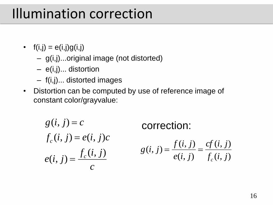
Illumination correction

• f(i,j) = e(i,j)g(i,j)

– g(i,j)...original image (not distorted)

– e(i,j)... distortion

– f(i,j)... distorted images

• Distortion can be computed by use of reference image of

constant color/grayvalue:

c

jifjie

cjiejif

cjig

c

c

),(),(

),(),(

),(

),(

),(

),(

),(),(

jif

jicf

jie

jifjig

c

correction:

16

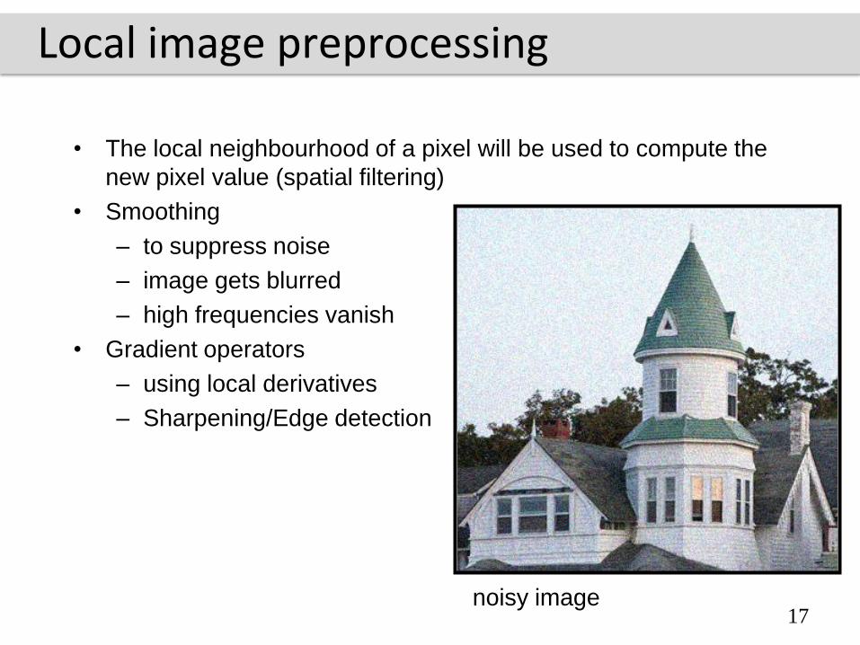
Local image preprocessing

• The local neighbourhood of a pixel will be used to compute the

new pixel value (spatial filtering)

• Smoothing

– to suppress noise

– image gets blurred

– high frequencies vanish

• Gradient operators

– using local derivatives

– Sharpening/Edge detection

17noisy image

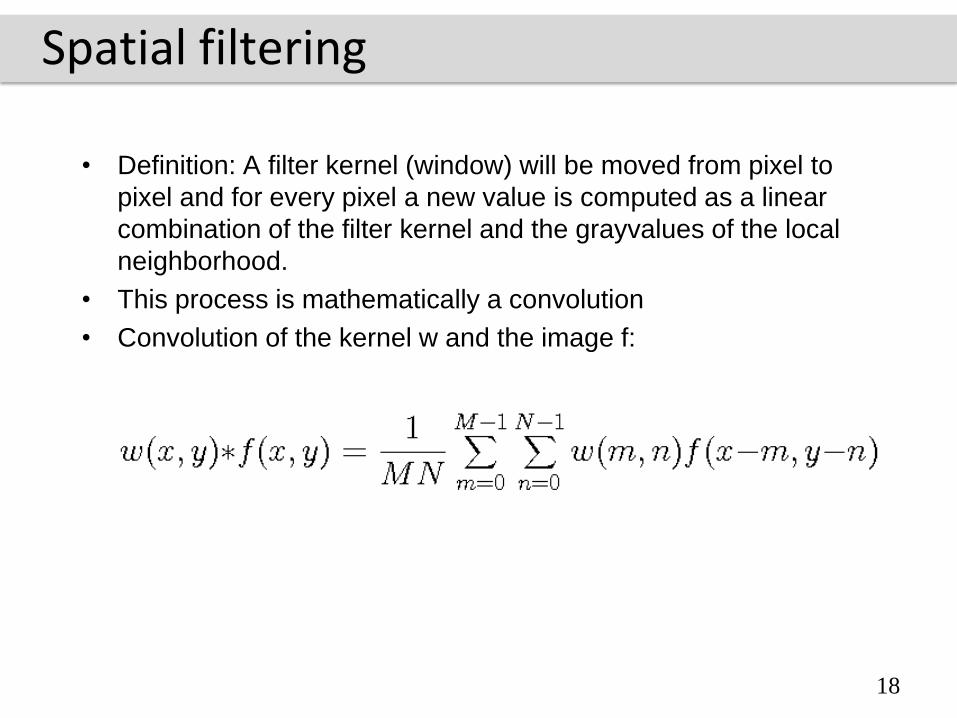
Spatial filtering

• Definition: A filter kernel (window) will be moved from pixel to

pixel and for every pixel a new value is computed as a linear

combination of the filter kernel and the grayvalues of the local

neighborhood.

• This process is mathematically a convolution

• Convolution of the kernel w and the image f:

18

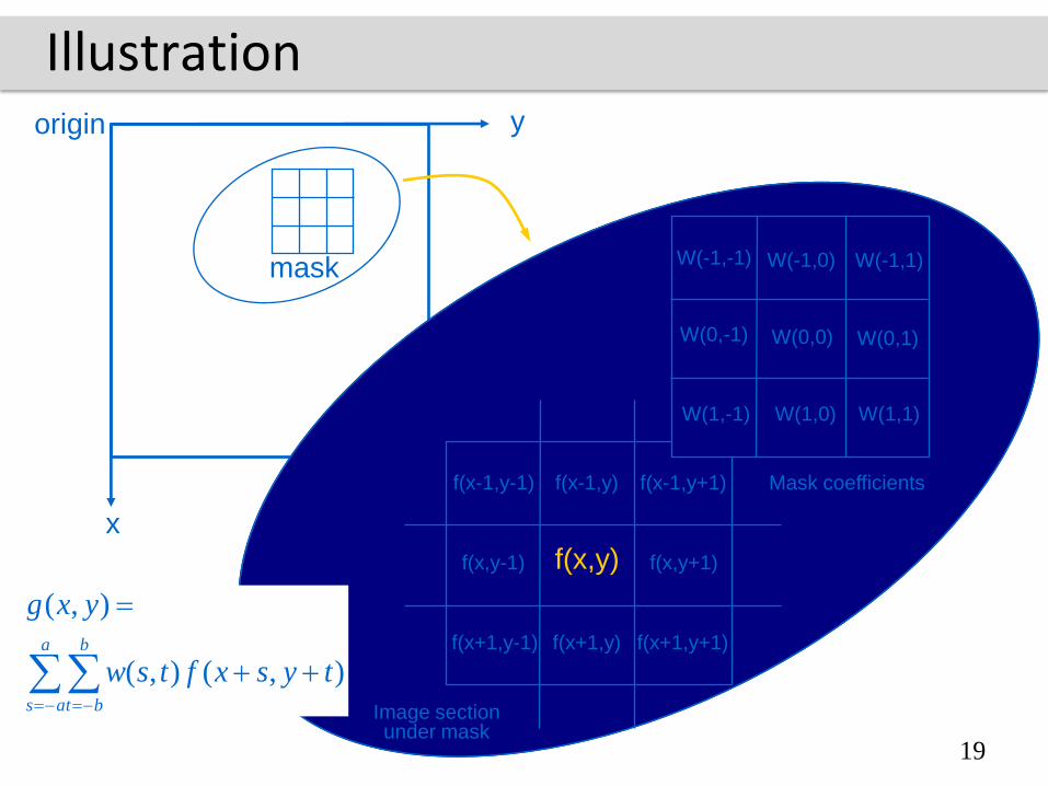
Illustration

W(-1,-1) W(-1,0) W(-1,1)

W(0,-1) W(0,0) W(0,1)

W(1,-1) W(1,0) W(1,1)

f(x-1,y-1) f(x-1,y) f(x-1,y+1)

f(x,y-1) f(x,y) f(x,y+1)

f(x+1,y-1) f(x+1,y) f(x+1,y+1)

x

yorigin

mask

Mask coefficients

Image section under mask

),(),(

),(

tysxftsw

yxg

a

as

b

bt

19

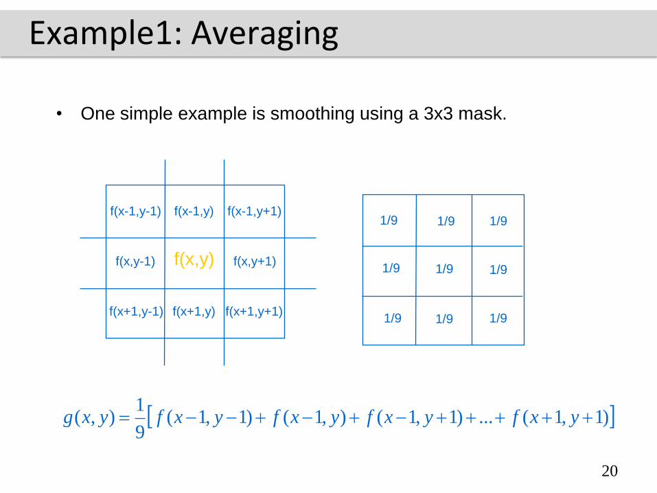
Example1: Averaging

• One simple example is smoothing using a 3x3 mask.

f(x-1,y-1) f(x-1,y) f(x-1,y+1)

f(x,y-1) f(x,y) f(x,y+1)

f(x+1,y-1) f(x+1,y) f(x+1,y+1)

1/9 1/91/9

1/9 1/9 1/9

1/9 1/9 1/9

)1,1(...)1,1(),1()1,1(9

1),( yxfyxfyxfyxfyxg

20

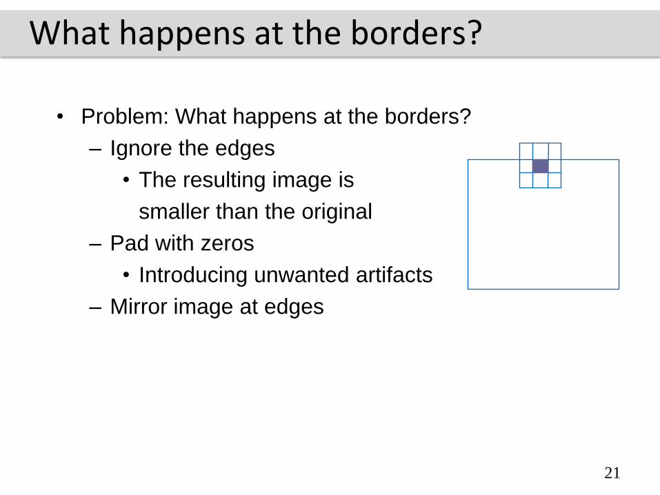
What happens at the borders?

• Problem: What happens at the borders?

– Ignore the edges

• The resulting image is

smaller than the original

– Pad with zeros

• Introducing unwanted artifacts

– Mirror image at edges

21

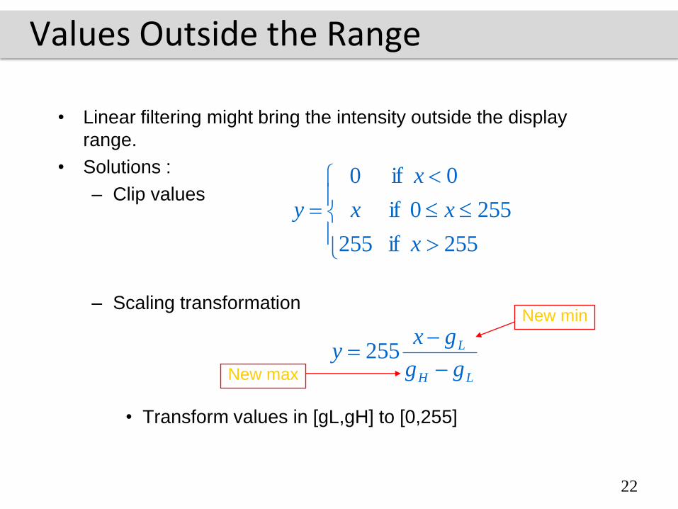
Values Outside the Range

• Linear filtering might bring the intensity outside the display

range.

• Solutions :

– Clip values

– Scaling transformation

• Transform values in [gL,gH] to [0,255]

255 if

2550 if

0 if

255

0

x

x

x

xy

LH

L

gg

gxy

255

New min

New max

22

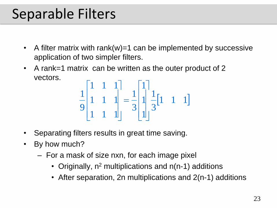
Separable Filters

• A filter matrix with rank(w)=1 can be implemented by successive

application of two simpler filters.

• A rank=1 matrix can be written as the outer product of 2

vectors.

• Separating filters results in great time saving.

• By how much?

– For a mask of size nxn, for each image pixel

• Originally, n2 multiplications and n(n-1) additions

• After separation, 2n multiplications and 2(n-1) additions

1113

1

1

1

1

3

1

111

111

111

9

1

23

Some terminology on Frequency…

• Frequencies: a measure of the amount by which gray values

change with distance.

• High/low-frequency components: large/small changes in gray

values over small distances.

• High/low-pass filter: passing high/low components, and reducing

or eliminating low/high-frequency filter.

24

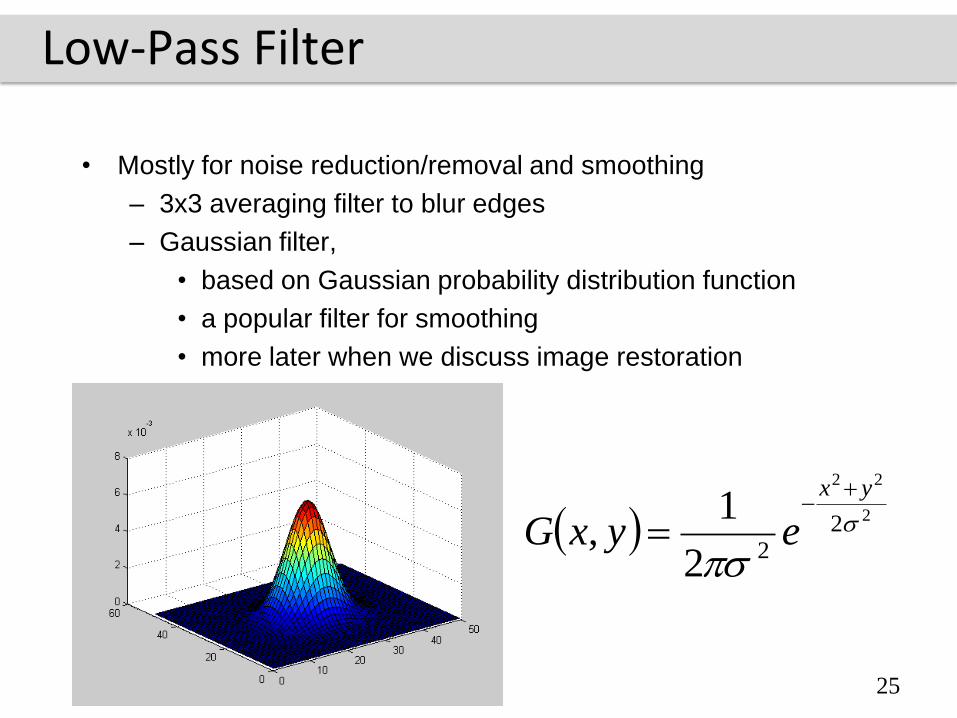
Low-Pass Filter

• Mostly for noise reduction/removal and smoothing

– 3x3 averaging filter to blur edges

– Gaussian filter,

• based on Gaussian probability distribution function

• a popular filter for smoothing

• more later when we discuss image restoration

2

22

222

1,

yx

eyxG

25

Gauss filtering

• A Gaussian filter is a weighted average filter. Pixel in the center

of the filter window are weighted stronger than pixel on the

border (according to the Gaussian distribution).

• The only parameter is (sigma), which is the standard

deviation. This value controls the degree of smoothing.

– as this parameter goes up, more pixels in the neighborhood

are involved in “averaging”,

– the image gets more blurred, and

– noise is more effectively suppressed

26

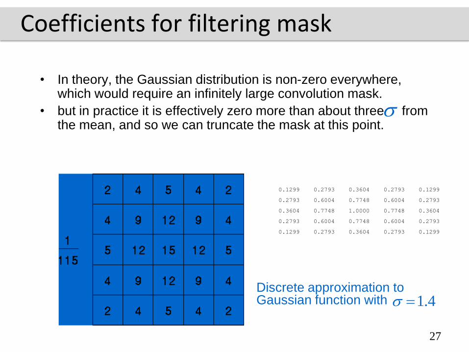
Coefficients for filtering mask

• In theory, the Gaussian distribution is non-zero everywhere, which would require an infinitely large convolution mask.

• but in practice it is effectively zero more than about three from the mean, and so we can truncate the mask at this point.

Discrete approximation to Gaussian function with 4.1

0.1299 0.2793 0.3604 0.2793 0.1299

0.2793 0.6004 0.7748 0.6004 0.2793

0.3604 0.7748 1.0000 0.7748 0.3604

0.2793 0.6004 0.7748 0.6004 0.2793

0.1299 0.2793 0.3604 0.2793 0.1299

1299 0.2793 0.

27

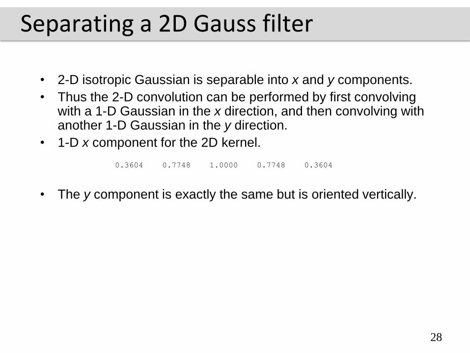
Separating a 2D Gauss filter

• 2-D isotropic Gaussian is separable into x and y components.

• Thus the 2-D convolution can be performed by first convolving with a 1-D Gaussian in the x direction, and then convolving with another 1-D Gaussian in the y direction.

• 1-D x component for the 2D kernel.

• The y component is exactly the same but is oriented vertically.

0.3604 0.7748 1.0000 0.7748 0.3604

1299 0.2793 0.

28

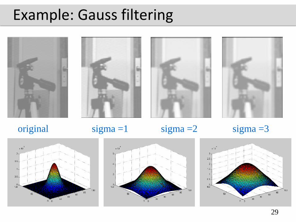
Example: Gauss filtering

sigma =1 sigma =2 sigma =3original

29

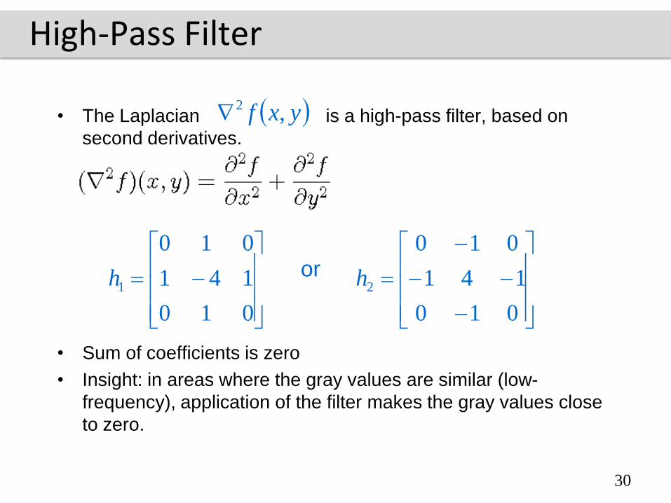
High-Pass Filter

• The Laplacian is a high-pass filter, based on

second derivatives.

• Sum of coefficients is zero

• Insight: in areas where the gray values are similar (low-

frequency), application of the filter makes the gray values close

to zero.

yxf ,2

010

141

010

2h

010

141

010

1h or

30

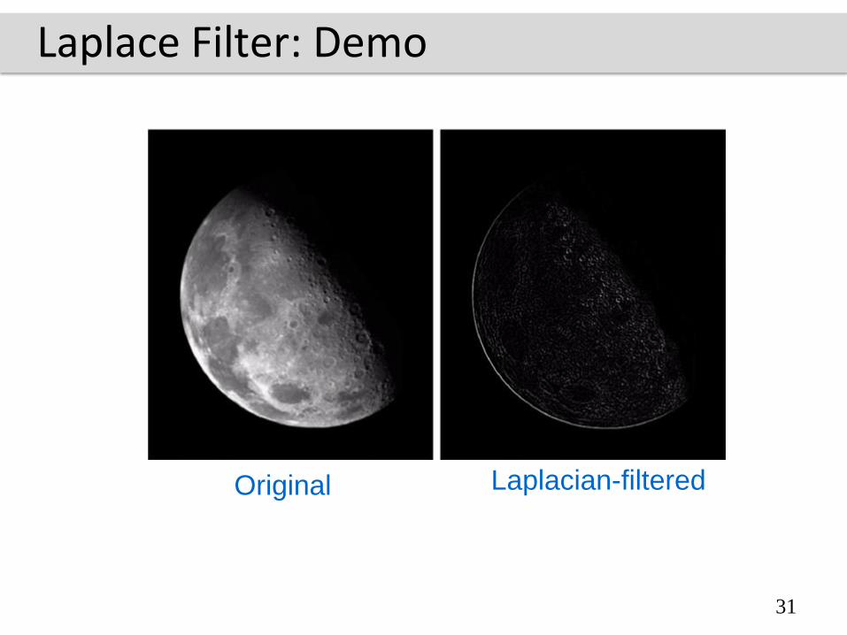
Laplace Filter: Demo

Original Laplacian-filtered

31

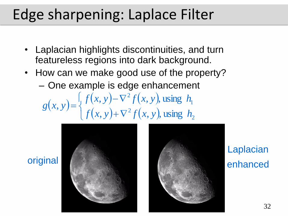
Edge sharpening: Laplace Filter

• Laplacian highlights discontinuities, and turn featureless regions into dark background.

• How can we make good use of the property?

– One example is edge enhancement

2

2

1

2

using ,,,

using ,,,,

hyxfyxf

hyxfyxfyxg

originalLaplacian

enhanced

32

Edge sharpening:Unsharp Masking

• To make edges slightly sharper and crisper.

• This operation is referred to as edge enhancement, edge

crispening or unsharp masking.

• A very popular practice in industry.

• Subtracting a blurred version of an image from the image itself.

, 2 , ,sf x y f x y f x y

Sharpened image

, , , ,sf x y f x y f x y f x y

Blurred imageOriginal image

Edge image

2

1, , ,

2sf x y f x y f x y

33

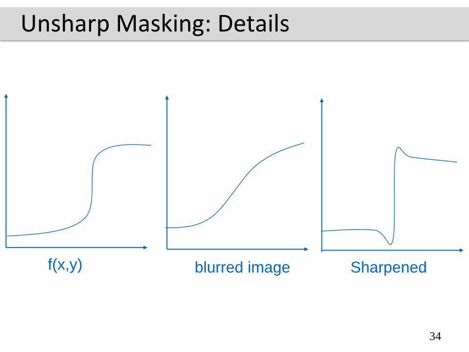
Unsharp Masking: Details

f(x,y) blurred image Sharpened

34

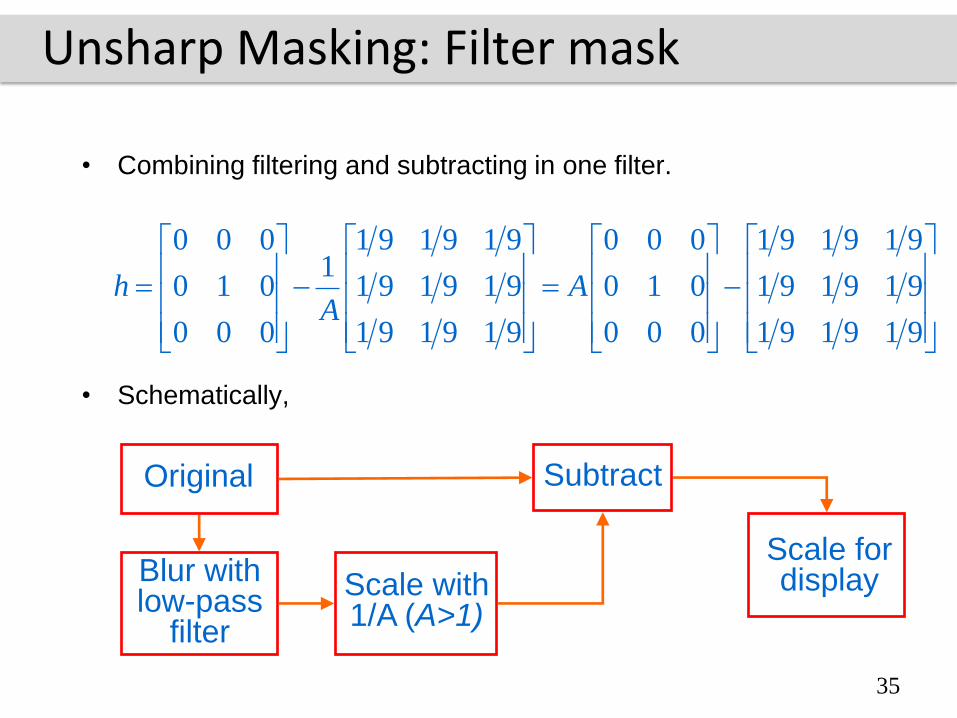
Unsharp Masking: Filter mask

• Combining filtering and subtracting in one filter.

• Schematically,

0 0 0 1 9 1 9 1 9 0 0 0 1 9 1 9 1 91

0 1 0 1 9 1 9 1 9 0 1 0 1 9 1 9 1 9

0 0 0 1 9 1 9 1 9 0 0 0 1 9 1 9 1 9

h AA

Original

Blur with low-pass

filter

Scale with 1/A (A>1)

Subtract

Scale for display

35

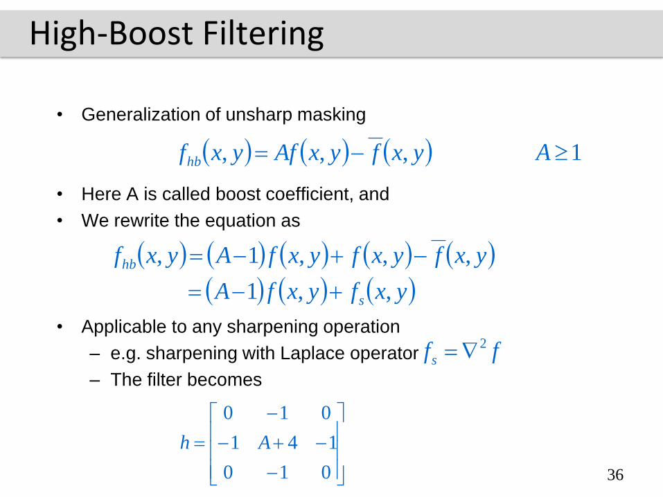
High-Boost Filtering

• Generalization of unsharp masking

• Here A is called boost coefficient, and

• We rewrite the equation as

• Applicable to any sharpening operation

– e.g. sharpening with Laplace operator

– The filter becomes

yxfyxAfyxfhb ,,, 1A

yxfyxfyxfAyxfhb ,,,1,

yxfyxfA s ,,1

2

sf f

010

141

010

Ah

36

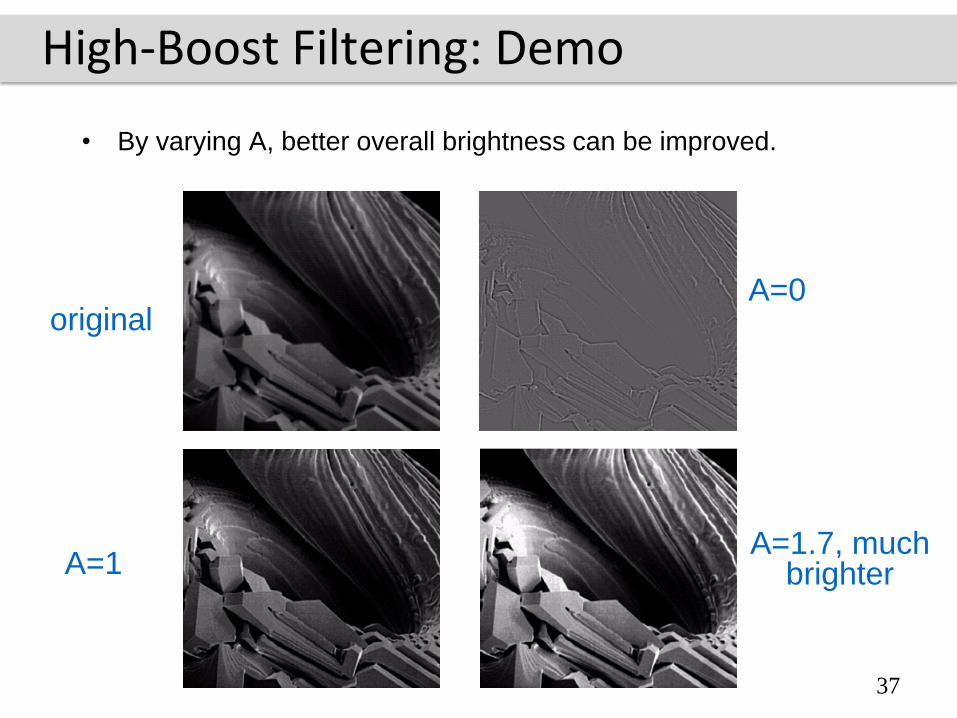
High-Boost Filtering: Demo

• By varying A, better overall brightness can be improved.

originalA=0

A=1A=1.7, much

brighter

37

Image Smoothing

• To suppress noise

• Computing an average of the grayvalues in a local

neighborhood

• Edges get blurred by averaging (high frequencies get

suppressed)

• Filter can be edge-preserving

• Averaging works well when single pixels are wrong

• Large noise regions (blobs) cannot really get removed

38

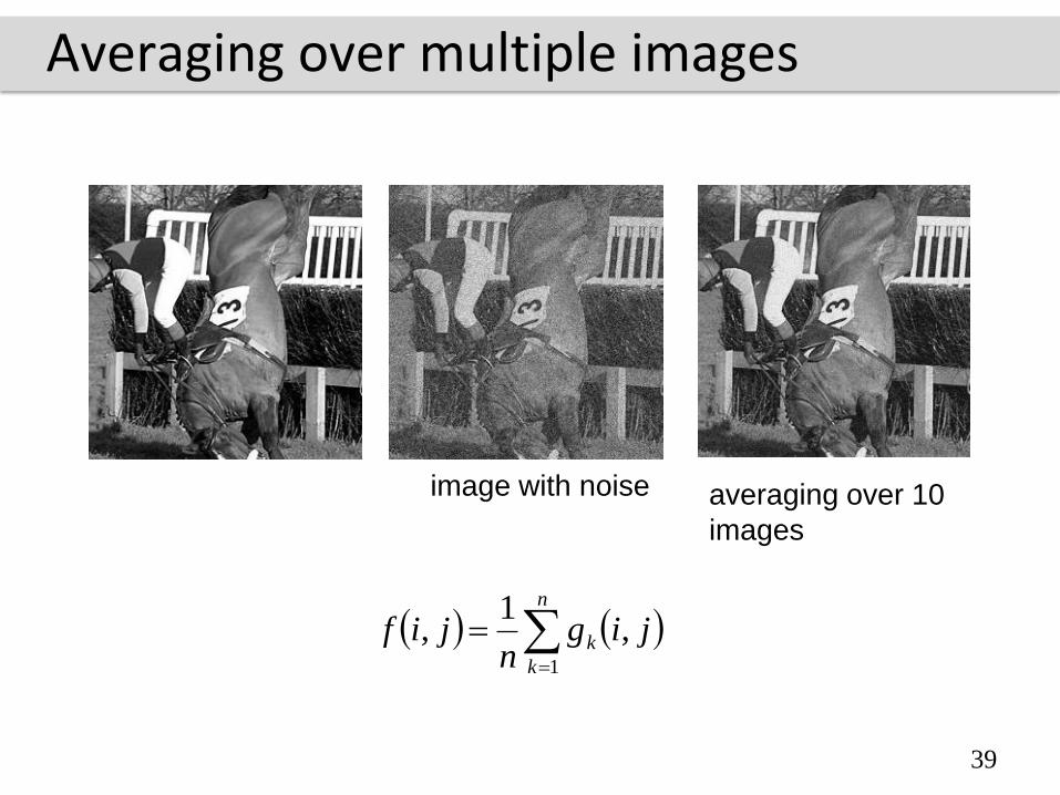
Averaging over multiple images

Original image with noise averaging over 10

images

n

k

k jign

jif1

,1

,

39

Spatial filtering

111

111

111

9

1h

1111111

1111111

1111111

1111111

1111111

1111111

1111111

49

1h

40

Spatial filtering

111

111

111

9

1h

111

121

111

10

1h

121

242

121

16

1h

Approximation of Gauss filtering

41

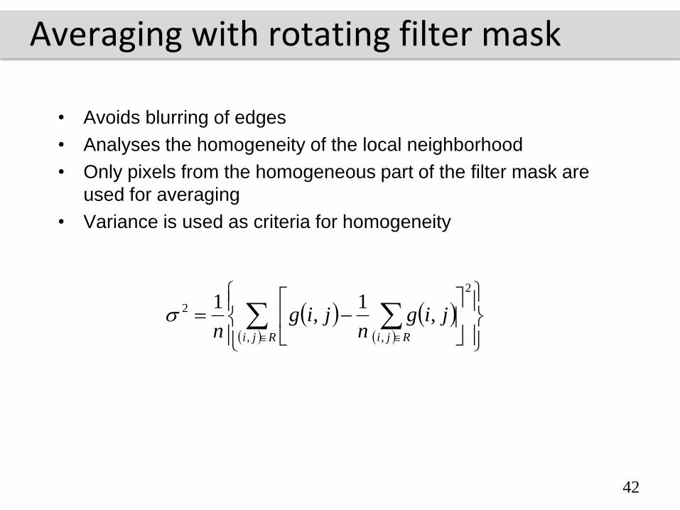
Averaging with rotating filter mask

• Avoids blurring of edges

• Analyses the homogeneity of the local neighborhood

• Only pixels from the homogeneous part of the filter mask are

used for averaging

• Variance is used as criteria for homogeneity

Rji Rji

jign

jign ,

2

,

2 ,1

,1

42

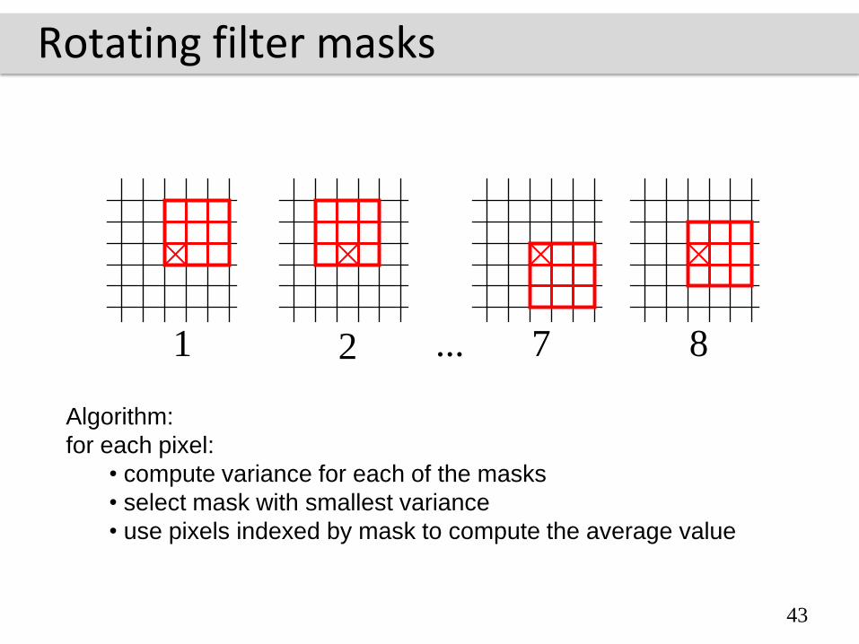
Rotating filter masks

1 2 7 8...

Algorithm:

for each pixel:

• compute variance for each of the masks

• select mask with smallest variance

• use pixels indexed by mask to compute the average value

43

Nonlinear Filters

• Maximum filter: the output the maximum value under

the mask

• Minimum filter: the output the minimum value under

the mask

• Rank-order filter:

– Elements under the mask are ordered, and a

particular value is returned.

– Both maximum and minimum filter are instances

of rank-order

– Another popular instance is median filter

44

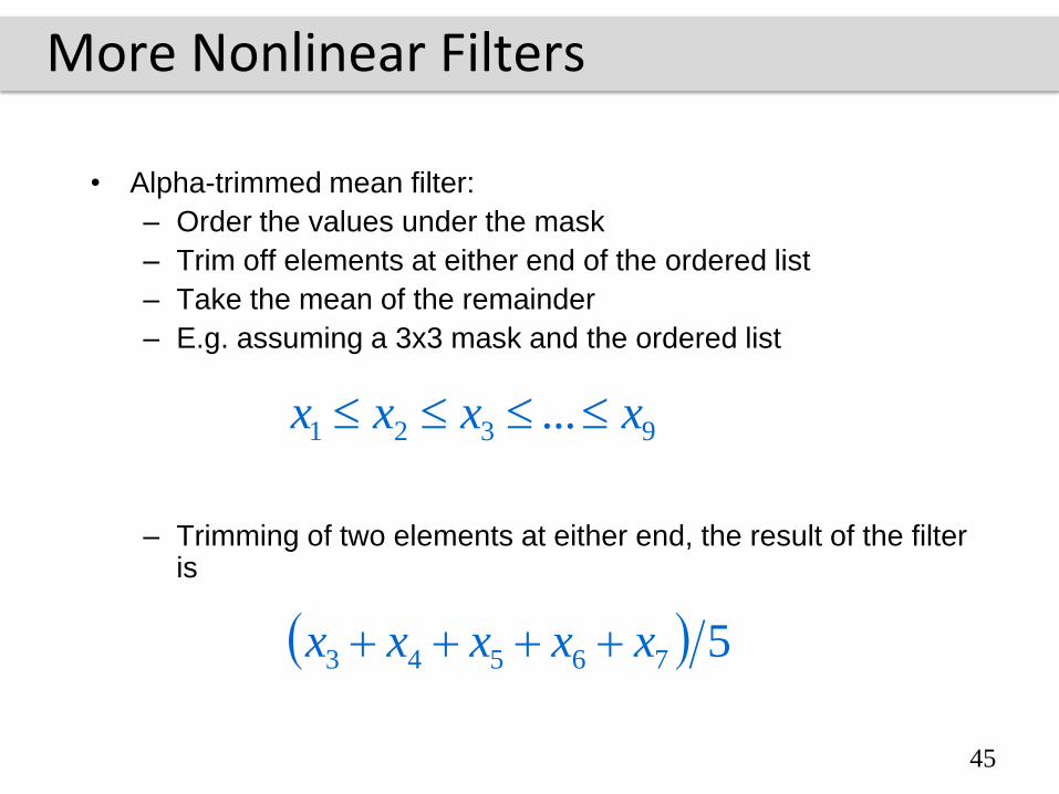
More Nonlinear Filters

• Alpha-trimmed mean filter:

– Order the values under the mask

– Trim off elements at either end of the ordered list

– Take the mean of the remainder

– E.g. assuming a 3x3 mask and the ordered list

– Trimming of two elements at either end, the result of the filter is

9321 ... xxxx

576543 xxxxx

45