1

Two types of t-tests:

Independent Measures (last week) & Repeated Measures

POPULATION

Random factors determine which group

n subjects

Group 1: N1 subject

Group 2: N2 subject

Level 1 of independent variable A given to all subjects (N1)

Level 2 of independent variable A given to all subjects (N2)

Group 1 subjects measured on dependent variable B

Group 2 subjects measured on dependent variable B

Compute ŝ1

!

X 1

!

X 2Compute ŝ2 Test your hypothesis

H0: µ1 – µ2 = 0 H1: µ1 – µ2 ≠ 0

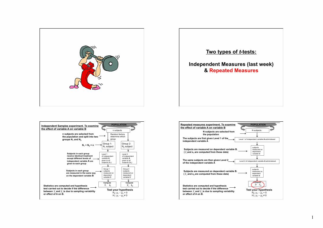
Independent Samples experiment. To examine the effect of variable A on variable B

n subjects are selected from the population and split into two groups N1 and N2

N1 + N2 = n

Subjects in each group receive identical treatment except different levels of independent variable A are given to each group

Subjects in each group are measured in the same way on the dependent variable B

Statistics are computed and hypothesis test carried out to decide if the difference between and is due to sampling variability or effect of A on B.

!

X 1

!

X 2

POPULATION

N subjects

Level 1 of independent variable A administered

subjects measured on dependent variable B

Compute

Test your hypothesis H0: µ1 – µ2 = 0 H1: µ1 – µ2 ≠ 0

Repeated measures experiment. To examine the effect of variable A on variable B N subjects are selected from

the population

Statistics are computed and hypothesis test carried out to decide if the difference between and is due to sampling variability or effect of A on B.

!

X 1

!

X 2

Level 2 of independent variable A administered

subjects measured on dependent variable B

!

D

The subjects are first given Level 1 of the independent variable A

The same subjects are then given Level 2 of the independent variable A

Subjects are measured on dependent variable B. ( and s1 are computed from these data)

!

X 1

Subjects are measured on dependent variable B. ( and s2 are computed from these data)

!

X 2

!

SD

2

Both types of t-test have one independent variable, with two levels (the two different conditions of our experiment). There is one dependent variable (the thing we actually measure). Example 1: Effects of personality type on a memory test. -Independent Variable is “personality type”;

Two levels - introversion and extraversion. -Dependent Variable is memory test score. Use an independent-measures t-test: measure each subject's memory score once, then compare introverts and extraverts. Example 2: Effects of alcohol on reaction-time (RT) performance. -Independent Variable is “alcohol consumption”;

Two levels - drunk and sober. -Dependent Variable is RT. Use a repeated-measures t-test: measure each subject's RT twice, once while drunk and once while sober.

Accuracy of Olympic marksmen/markswomen

Shots fired between heartbeats versus during a heartbeat (repeated measures design)

Rationale behind repeated measures the t-test:

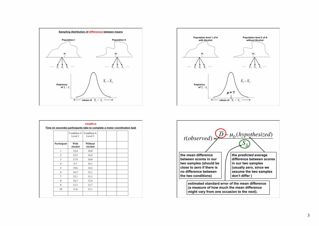
EXAMPLE: Experiment on the effect of alcohol on task performance (time in seconds).

Measure time taken to perform the task for subjects when drunk, and when (same subjects are) sober.

Null hypothesis: alcohol has no effect on time taken: variation between the drunk sample mean and the sober sample mean is due to sampling variation.

i.e. The drunk and sober performance times are samples from the same population.

From the lecture on sampling distribution:

!

"X ="N

µ = 63 in. σ = 2 in.

3

Sampling distribution of differences between means

Population I Population II

!

X 2

!

X 1. . . . . . . . . . . .

!

X 1

!

X 1

!

X 2

!

X 2

µ1 µ2

frequency of

!

X 1

!

X 2values of −

X1 ! X2X1 ! X2

Population level 1 of A with Alcohol

!

X 2

!

X 1. . . . . . . . . . . .

!

X 1

!

X 1

!

X 2

!

X 2

µ1 µ2

!

X 1

!

X 2values of −

Population level 2 of A without Alcohol

µ = ?

X1 ! X2frequency

of X1 ! X2

Condition A Level 1

Condition A Level 2

Participant With Alcohol

Without Alcohol

1 12.4 10.0

2 15.5 14.2

3 17.9 18.0

4 9.7 10.1

5 19.6 14.2

6 16.5 12.1

7 15.1 15.1

8 16.3 12.4

9 13.3 12.7

10 11.6 13.1

Time (in seconds) participants take to complete a motor coordination task EXAMPLE

the mean difference between scores in our two samples (should be close to zero if there is no difference between the two conditions)

the predicted average difference between scores in our two samples (usually zero, since we assume the two samples don’t differ )

estimated standard error of the mean difference (a measure of how much the mean difference might vary from one occasion to the next).

!

t(observed) =D "µD (hypothesized)

SD

4

Condition A Level 1

Condition A Level 2

Participant With Alcohol

Without Alcohol

Diff. (D)

1 12.4 10.0 2.4

2 15.5 14.2 1.3

3 17.9 18.0 -0.1

4 9.7 10.1 -0.4

5 19.6 14.2 5.4

6 16.5 12.1 4.4

7 15.1 15.1 0.0

8 16.3 12.4 3.9

9 13.3 12.7 0.6

10 11.6 13.1 -1.5

16.0

!

D" =

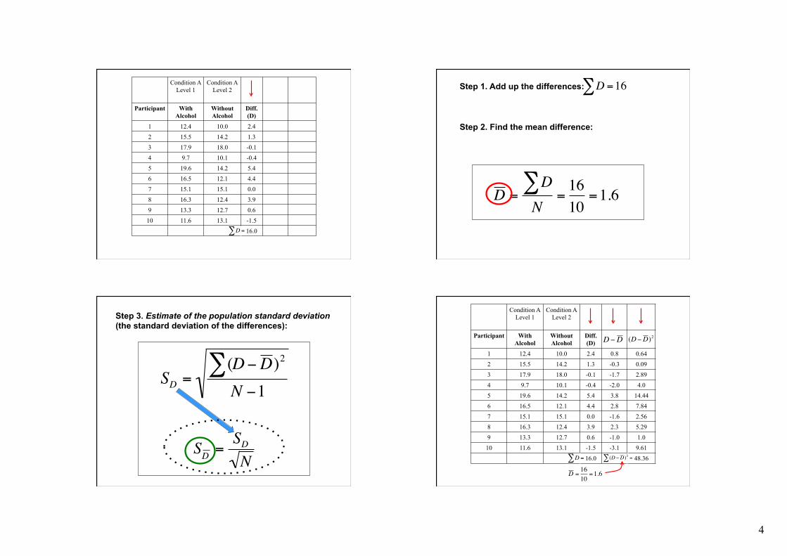
Step 1. Add up the differences:

Step 2. Find the mean difference:

!

D =16"

!

D =D"

N=1610

=1.6

Step 3. Estimate of the population standard deviation (the standard deviation of the differences):

!

SD =(" D#D )2

N #1

!

SD =SD

N

Condition A Level 1

Condition A Level 2

Participant With Alcohol

Without Alcohol

Diff. (D)

1 12.4 10.0 2.4 0.8 0.64

2 15.5 14.2 1.3 -0.3 0.09

3 17.9 18.0 -0.1 -1.7 2.89

4 9.7 10.1 -0.4 -2.0 4.0

5 19.6 14.2 5.4 3.8 14.44

6 16.5 12.1 4.4 2.8 7.84

7 15.1 15.1 0.0 -1.6 2.56

8 16.3 12.4 3.9 2.3 5.29

9 13.3 12.7 0.6 -1.0 1.0

10 11.6 13.1 -1.5 -3.1 9.61

16.0 48.36

!

D"D

!

(D"D )2

!

D" =

!

(D"D )2 =#

!

D = 1610

=1.6

5

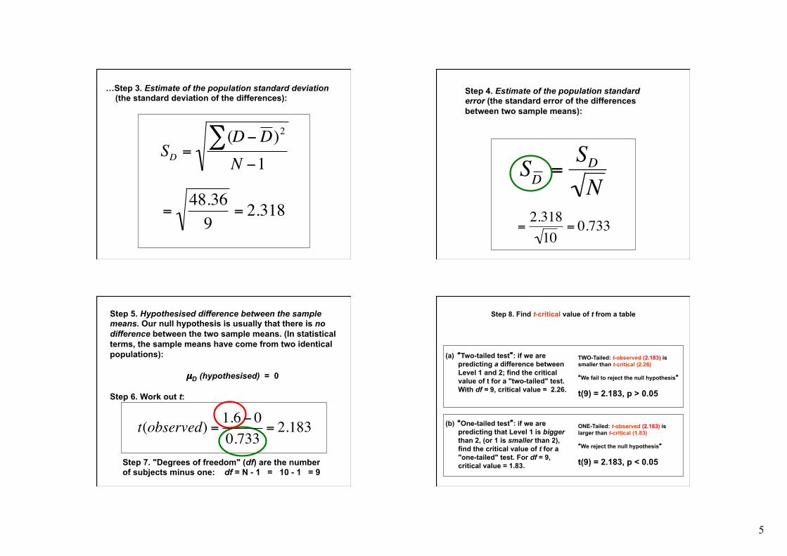
…Step 3. Estimate of the population standard deviation (the standard deviation of the differences):

!

SD =(" D#D )2

N #1

!

=48.369

= 2.318

Step 4. Estimate of the population standard error (the standard error of the differences between two sample means):

!

SD =SD

N

!

=2.31810

= 0.733

Step 5. Hypothesised difference between the sample means. Our null hypothesis is usually that there is no difference between the two sample means. (In statistical terms, the sample means have come from two identical populations):

µD (hypothesised) = 0 Step 6. Work out t:

Step 7. "Degrees of freedom" (df) are the number of subjects minus one: df = N - 1 = 10 - 1 = 9

!

t(observed) =1.6 " 00.733

= 2.183

(a)  “Two-tailed test”: if we are predicting a difference between Level 1 and 2; find the critical value of t for a "two-tailed" test. With df = 9, critical value = 2.26.

(b)   “One-tailed test”: if we are predicting that Level 1 is bigger than 2, (or 1 is smaller than 2), find the critical value of t for a "one-tailed" test. For df = 9, critical value = 1.83.

TWO-Tailed: t-observed (2.183) is smaller than t-critical (2.26) “We fail to reject the null hypothesis”

t(9) = 2.183, p > 0.05

ONE-Tailed: t-observed (2.183) is larger than t-critical (1.83) “We reject the null hypothesis”

t(9) = 2.183, p < 0.05

Step 8. Find t-critical value of t from a table

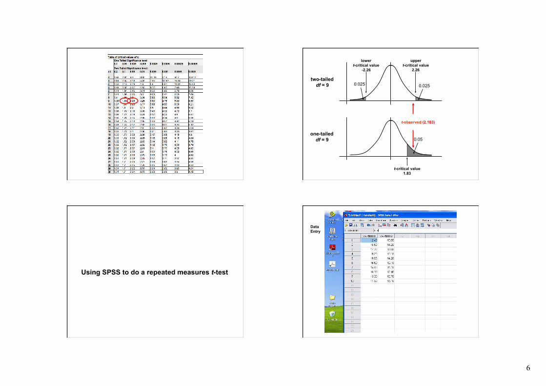
6

0.025 0.025

upper t-critical value

2.26

lower t-critical value

-2.26

two-tailed df = 9

one-tailed df = 9 0.05

t-critical value 1.83

t-observed (2.183)

Using SPSS to do a repeated measures t-test

Data Entry

7

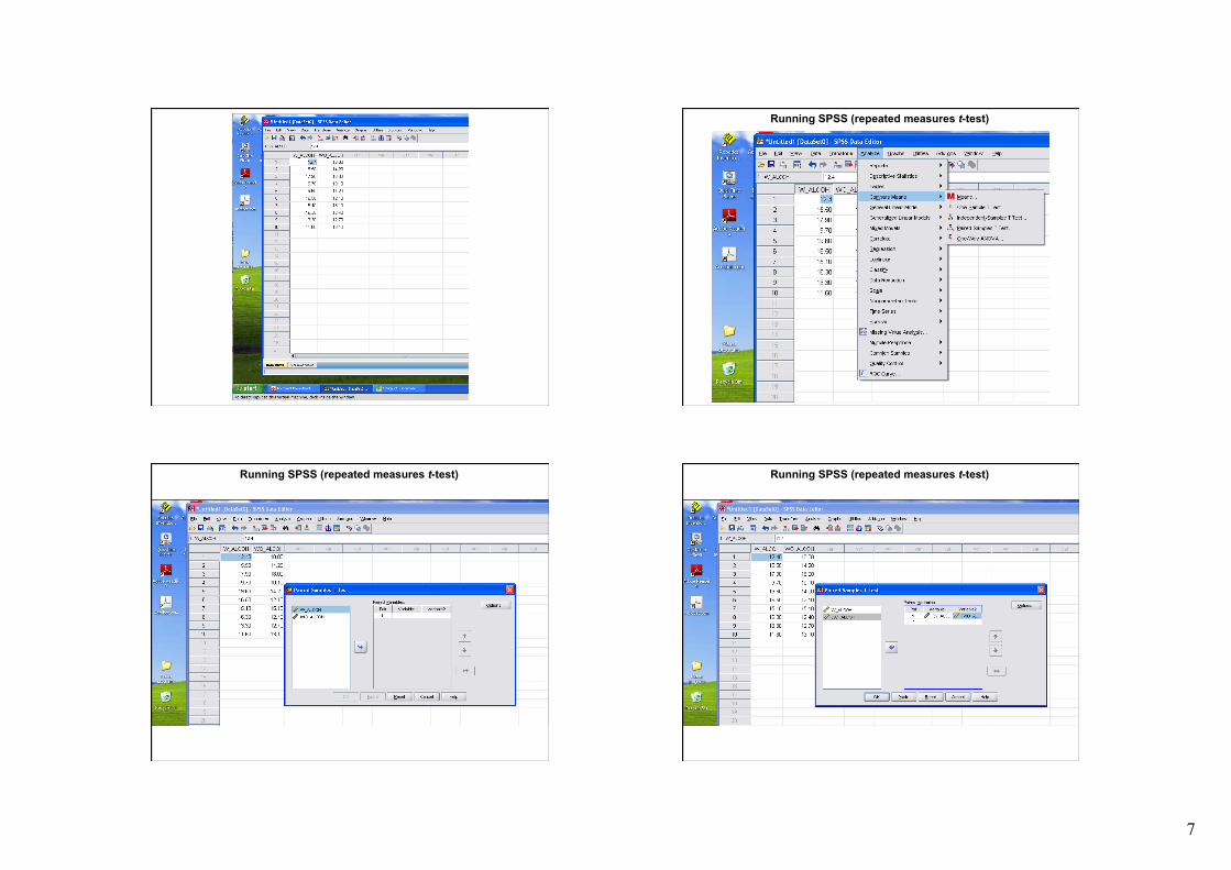
Running SPSS (repeated measures t-test)

Running SPSS (repeated measures t-test) Running SPSS (repeated measures t-test)

8

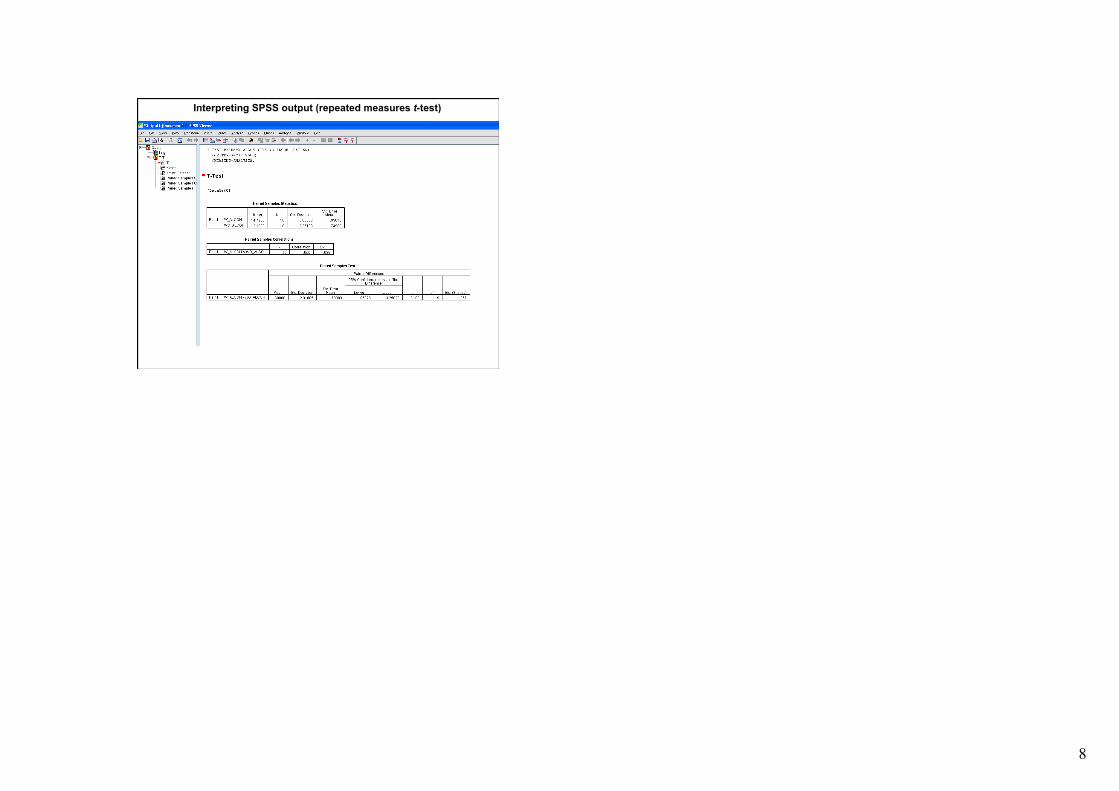
Interpreting SPSS output (repeated measures t-test)