4. three theorems malvino text continued - …wevans/excerpts_malvino_4.pdf · 1 4. three theorems...
TRANSCRIPT

1
4. Three Theorems – Malvino Text Continued A theorem is a mathematically provable statement. In this book, the word “theorem” is used only when something important is said about electrical quantities. This chapter discusses three theorems. The first is a shortcut, not really essential, but useful in many circuits. The next two theorems help us rearrange and simplify circuits. In fact, the second and third theorems of this chapter are so crucial that without them it is impossible to have a deep understanding of circuits. These theorems are so vital we discuss them intensively in this chapter and apply them constantly in later chapters. Furthermore, when you get to electronics, you will find the last two theorems of this chapter are the keys to transistor-circuit analysis. 4-1. Voltage-Divider Theorem The voltage from a source may be more than you need. To reduce voltage, you can use a voltage divider. V is the input voltage and V2 is the output voltage. Since charges lose potential energy passing through R1, the output voltage is less than the input. The two main questions in this section answers are
What is the voltage-divider theorem? How does a potentiometer work?
Formula for output voltage Here is how to derive a formula for V2. In Fig. 4-1a,
V2 = R2I
V= (R1+R2)·I ratio of these two equations is
V2
V=
R2
R1 + R2
or V2
V=
R2
R
where R = R1 + R2, the equivalent resistance between the input terminals. Multiplying both sides of Eq.
(4-1a) by V gives
V2 =R2
RV
2
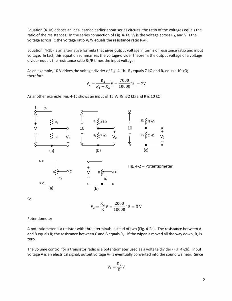
Equation (4-1a) echoes an idea learned earlier about series circuits: the ratio of the voltages equals the ratio of the resistances. In the series connection of Fig. 4-1a, V2 is the voltage across R2, and V is the voltage across R; the voltage ratio V2/V equals the resistance ratio R2/R. Equation (4-1b) is an alternative formula that gives output voltage in terms of resistance ratio and input voltage. In fact, this equation summarizes the voltage-divider theorem; the output voltage of a voltage divider equals the resistance ratio R2/R times the input voltage. As an example, 10 V drives the voltage divider of Fig. 4-1b. R2 equals 7 kΩ and RT equals 10 kΩ; therefore,
V2 =R2
𝑅1 + 𝑅2V =
7000
1000010 = 7V
As another example, Fig. 4-1c shows an input of 15 V. R2 is 2 kΩ and R is 10 kΩ.
I
(a) (b)
R1 3 k +
V
--R2
+
V2
--
+
10
-- +
V2
--
7 k
(c)
8 k +
10
-- +
V2
--
2 k
R1
R2
R1
R2
A
B
R
R2
C
(a)
R
R2
C
(b)
+
V
--
Fig. 4-2 – Potentiometer
So,
V2 =R2
RV =
2000
1000015 = 3 V
Potentiometer A potentiometer is a resistor with three terminals instead of two (Fig. 4-2a). The resistance between A and B equals R; the resistance between C and B equals R2. If the wiper is moved all the way down, R2 is zero. The volume control for a transistor radio is a potentiometer used as a voltage divider (Fig. 4-2b). Input voltage V is an electrical signal; output voltage V2 is eventually converted into the sound we hear. Since
V2 =R2
RV

3
we can control the volume or strength of the sound by moving the wiper. Adjustable voltage dividers like Fig. 4-2b are widely used in radio, TV, measuring instruments, etc. Example 4-1 In Fig. 4-3a, what are the minimum and maximum output voltages? The output voltage when the wiper is in the middle? With the wiper all the way down, we tap off zero resistance and the output voltage equals
V2 =R2
RV =
0
RV = 0 V
When the wiper is at the top, R2 equals R and the output voltage is
V2 =R2
RV =
5,000
10,0002 = 2 V
Example 4-2 What is the equivalent resistance between the input terminals of Fig. 4-3b? The resistances are in series. So, R = 900,000 + 90,000 + 9,000 + 1,000 = 1,000,000 Ω = 1 M Ω
Example 4-3 In Fig. 4-3b, when the switch is moved to different positions, different output voltages result. Calculate the output voltage for each position A through E. Similar to Example 4-1, R1 equals zero means V2 is zero; R2 equals R means V2 is equal to V. Therefore, position A gives a 10 V output and position E gives a zero output.
10 k
(a)
+
2
--
Fig. 4-3
+
V2
--
900 k
+
10 V
--
+
V2
--
90 k
9 k
1 k
A
B
C
D
E
(b)

4
In position D, R2 equals 1 kΩ and
V2 =R2
RV =
1,000
1,000,00010 = 10 mV
For position C, R2 is 10 kΩ and
V2 =10,000
1,000,00010 = 0.1 V = 100 mV
Position B has an R2 of 100 kΩ and
V2 =100,000
1,000,00010 = 1 V
The output voltage changes in decade steps by a factor of 10: 10 mV, 100 mV, 1 V and 10 V. Many electronic instruments use decade-step voltage dividers like Fig. 4-3b. 4-2 Thevenin Quantities When analyzing an electronic circuit, you seldom have to find all voltages and currents in the circuit; most of the time you will be after the voltage or current for a single resistance. When this is the case, Thevenin’s theorem is often the easiest way to a solution. Without doubt, this theorem tops the list for importance; experienced technicians and engineers have used it thousands of times. Section 4-3 states the Thevenin theorem and the conditions that must be satisfied when you apply it. Before you can understand the theorem, you first need to learn the answers to: What is Thevenin voltage? What is Thevenin resistance? What is a Thevenin circuit?

5
(a)(b)
Fig. 4-4 Thevenin quantities
6 k A
+
12 V
--3 k
B
2 k
6 k A
+
12 V
--3 k
B
+
Vth
--
(d)
2 k A
+
4 V
--
B
(c)
6 k A
3 k
B
+
Rth
--
Thevenin voltage The Thevenin voltage between a pair of terminals is defined as the voltage that results when the load between these terminals is opened. For instance, Fig. 4-4a shows a 2-kΩ load between the A-B terminals. If the load is opened (removed), the circuit reduces to Fig. 4-4b. By definition, the voltage appearing between the A-B terminals of this open-load circuit is called the Thevenin voltage Vth. Figure 4-4b is a voltage divider. So, in this particular case, the Thevenin voltage equals
Vth =R2
RV =
3,000
9,00012 = 4 V
Thevenin resistance The Thevenin resistance between a pair of terminals is defined as the resistance between these terminals when the load is open and the source reduced to zero. In Fig. 4-4b, the load is open; if we now visualize the source reduced to zero, the circuit simplifies to Fig. 4-4c. By definition, the resistance between the A-B terminals of this zero-source circuit is called the Thevenin resistance. (Note: reducing a voltage source to zero is the same as replacing it by zero resistance, because R=0 means V=RI = 0.) The 6-kΩ resistor in Fig. 4-4c is in parallel with the 3 kΩ resistor, because both resistors are between the same pair of equipotential points. Therefore, in this particular case, the Thevenin resistance equals
Rth =6000 × 3000
6000 + 3000= 2 kΩ
6
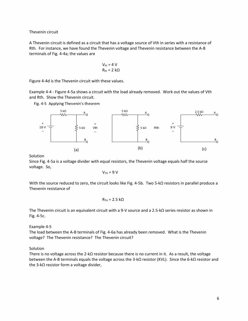
Thevenin circuit A Thevenin circuit is defined as a circuit that has a voltage source of Vth in series with a resistance of Rth. For instance, we have found the Thevenin voltage and Thevenin resistance between the A-B terminals of Fig. 4-4a; the values are Vth = 4 V Rth = 2 kΩ Figure 4-4d is the Thevenin circuit with these values. Example 4-4 - Figure 4-5a shows a circuit with the load already removed. Work out the values of Vth and Rth. Show the Thevenin circuit.
(a) (b)
Fig. 4-5 Applying Thevenin s theorem
5 k A
+
18 V
--5 k
B
+
Vth
--
2.5 k A
+
9 V
--
B
(c)
5 k A
5 k
B
Rth
Solution Since Fig. 4-5a is a voltage divider with equal resistors, the Thevenin voltage equals half the source voltage. So, VTH = 9 V With the source reduced to zero, the circuit looks like Fig. 4-5b. Two 5-kΩ resistors in parallel produce a Thevenin resistance of RTH = 2.5 kΩ The Thevenin circuit is an equivalent circuit with a 9-V source and a 2.5-kΩ series resistor as shown in Fig. 4-5c. Example 4-5 The load between the A-B terminals of Fig. 4-6a has already been removed. What is the Thevenin voltage? The Thevenin resistance? The Thevenin circuit? Solution There is no voltage across the 2-kΩ resistor because there is no current in it. As a result, the voltage between the A-B terminals equals the voltage across the 3-kΩ resistor (KVL). Since the 6-kΩ resistor and the 3-kΩ resistor form a voltage divider,

7
(a) (b)
Fig. 4-6 Another eample of Thevenin s theorem
6 k A
+
15 V
--3 k
B
+
Vth
--
4 k A
+
5 V
--
B
(c)
Rth
2 k 6 k A
3 k
B
2 k
Rth
A
2 k
B
2 k
(d)
Vth =R2
RV =
3,000
9,00015 = 5 V
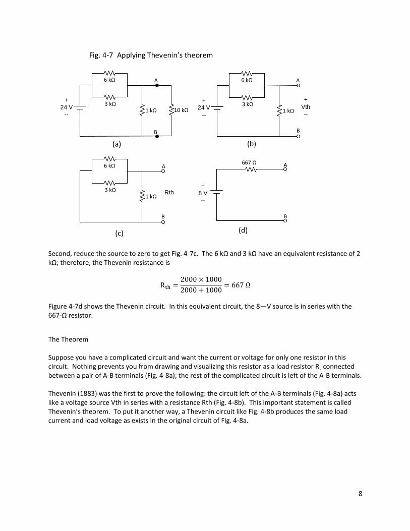
Next, get Rth. Figure 4-6b shows the circuit with the source reduced to zero. The 6-kΩ resistor and the 3-kΩ resistor are in parallel, because they are between the same pair of equipotential points. When these two resistors are combined, the circuit simplifies to Fig. 4-6c. The Thevenin resistance between the A-B terminals is Rth = 2 kΩ + 2 kΩ = 4 kΩ Fig. 4-6d shows the Thevenin circuit; it’s an equivalent circuit with a 5-V source in series with a 4-kΩ resistor. Example 4-6 Figure 4-7 shows a 10-kΩ load between the A-B terminals. Work out the Thevenin voltage, the Thevenin resistance, and show the Thevenin circuit. First, open the 10-kΩ resistor to get Fig. 4-7b. The parallel connection of 6 kΩ and 3 kΩ is equivalent to 2 kΩ. Therefore, the Thevenin voltage is
Vth =R2
RV =
1,000
3,00024 = 8 V
8
(a) (b)
Fig. 4-7 Applying Thevenin s theorem
A
+
24 V
--1 k
B
+
Vth
--
667 A
+
8 V
--
B
(c)
Rth
(d)
3 k
6 k
10 k
A
+
24 V
--1 k
B
3 k
6 k
1 k 3 k
6 k A
B
Second, reduce the source to zero to get Fig. 4-7c. The 6 kΩ and 3 kΩ have an equivalent resistance of 2 kΩ; therefore, the Thevenin resistance is
Rth =2000 × 1000
2000 + 1000= 667 Ω
Figure 4-7d shows the Thevenin circuit. In this equivalent circuit, the 8—V source is in series with the 667-Ω resistor.
The Theorem Suppose you have a complicated circuit and want the current or voltage for only one resistor in this circuit. Nothing prevents you from drawing and visualizing this resistor as a load resistor RL connected between a pair of A-B terminals (Fig. 4-8a); the rest of the complicated circuit is left of the A-B terminals. Thevenin (1883) was the first to prove the following: the circuit left of the A-B terminals (Fig. 4-8a) acts like a voltage source Vth in series with a resistance Rth (Fig. 4-8b). This important statement is called Thevenin’s theorem. To put it another way, a Thevenin circuit like Fig. 4-8b produces the same load current and load voltage as exists in the original circuit of Fig. 4-8a.

9
I
(a)
Fig. 4-8 Thevenin s theorem
A
B
+
Vth
--
Rth
RL
Circuit with sources and linear resistances
+
V
--
A
B
+
V
--
(b)
I
RL
Linearity and independent sources The proof of Thevenin’s theorem is too advanced to reproduce here. In the proof, however, are two critical conditions that must be satisfied when you apply the theorem. First, all resistances left of the A-B terminals in the original circuit (Fig. 4-8a) must be linear. (A 5-kΩ resistor has to have a constant value of 5-kΩ even though its voltage and current vary.) Unless this condition is satisfied, you cannot use Thevenin’s theorem. The linearity condition does not apply to RL; it can be linear or nonlinear. Second, only independent sources are reduced to zero when finding Rth; an independent source is one whose value is independent of any load voltage or load current in the original circuit. This book uses only independent sources; so when you find Rth, reduce all sources to zero. Example 4-7 discusses a dependent source.)
I
(a)
Fig. 4-10 Dependent and Independent sources
5 k
7 k
A
B
(b)
+
10
--9 k
6 k 8 k
+
2
--
2 k
+
10
--
7 k
4 k 6 k
+
10I
--
+
V
--
+
5V
--
Solution The value of an independent source does not depend on any load current or load voltage in the circuit. The sources in Fig. 4-10a have values of 10 V and 2 V; these values are constants and do not depend on voltage or current elsewhere in the circuit. Therefore, the sources are independent sources. In Fig. 4-10b, the source on the left has a value of 10 V, which in no way depends on the other voltages or currents; therefore, the left source is an independent source. But in the middle and right sources of Fig. 4-10b are different. I is the current through the 2-kΩ resistor; therefore, the 10I source has a value that does depend on the current in another part of the circuit. Also, V is the voltage across a 7-kΩ

10
resistor; therefore, the 5V source has a value that depends on another voltage. The 10I and 5V sources are examples of dependent sources. This is the last time you will encounter dependent voltage sources in this book; the rest of the book uses only independent sources, so no problems arise when reducing sources to zero. Later when you get into electronics, you will again see dependent sources; when you apply Thevenin’s theorem to these circuits, remember to reduce only the independent sources to zero; leave the dependent sources alone. Example 4-8 Find the values of V and I in Fig. 4-11a using Thevenin’s theorem. First, remove the load resistance to get the open-load circuit of Fig. 4-11b. In this open-load circuit, no charges flow through the 1-kΩ resistance. Kirchhoff’s voltage law implies Vth equals the voltage across the 3-kΩ resistance. With the voltage-divider theorem,
Vth =R2
RV =
3,000
9,00012 = 4 V
Second, reduce the 12-V source to zero to get the zero-source circuit of Fig. 4-11c. The 6-kΩ resistance is in parallel with the 3-kΩ resistance; these two combine into the equivalent 2- kΩ resistance of Fig. 4-11d. The Thevenin resistance between the terminals is RTH = 3 kΩ Third, draw the Thevenin circuit with the load connected (Fig. 4-11e). In this circuit
I =4
8000= 0.5 mA
The load voltage equals V = RLI = 5000 × 0.0005 = 2.5 V

11
(a)
Fig. 4-11 Example of Thevenin s Theorem
R1
6 k
3 k +
Vth
--
I
+
12
--
5 k
1 k
+
V
--
R2
R3
(b)
R1
6 k
3 k +
12
--
1 k
R2
R3
Rth
(c)
R1
6 k
3 k
1 k
R2
R3
Rth
(d)
2 k
1 k
(e)
3 k
+
4
--
I
5 k
+
V
-- RL
(f)
I
RL
Black box
If you were to analyze the original circuit (Fig. 4-11a), you would get exactly the same load current and load voltage for the 5-kΩ resistor. Example 4-9 A black box has a load resistance of RL connected to its output terminals as shown in Fig. 4-11f. When the load is opened, a voltmeter reads 15 V between the A-B terminals. When all sources inside the black box are reduced to zero, an ohmmeter measures 10 kΩ between the A-B terminals. What is the Thevenin circuit for the black box? Solution No matter what’s inside the black box, it acts the same as a 15-V source in series with a 10-kΩ resistance. In other words, no matter what you connect between the A-B terminals, you get exactly the same value of load current with the black box or the Thevenin circuit. The point is you can measure Vth and Rth in a built-up circuit; some circuits are extremely complicated, and it may be easier to measure the Thevenin quantities than to calculate them.

12
Example 4-10 – Solve for the value of I in Fig 4-12a:
(a)
Fig. 4-12 Applying Thevenin s Theorem more than once
4 k
4 k
I
+
18
--
6 k
1 k
8 k
A
B
C
D
(b)
4 k
4 k +
18
--
C
D
(c)
2 k
+
9
--
6 k
1 k A
B
C
D
3 k
4 k +
9
--
A
B
2 k
4 k
A
B
I
8 k +
6
--
(d)
(e) Solution: The key idea in this example is to apply Thevenin’s theorem more than once. The first application of Thevenin’s theorem is at the C-D terminals. When we open the C-D terminals, we get the open-loop circuit of Fig. 4-12b. The equal resistances give a Vth of 9 V. With a zero source, 4 kΩ gives an Rth of 2 kΩ. Therefore, we can replace the original circuit left of the C-D terminals by the Thevenin circuit shown in Fig. 4-12c. The resulting circuit is still not as simple as it can be. Combining the 2-kΩ and 1-kΩ resistances gives the 3-kΩ resistance of Fig. 4-12d. Applying the voltage-divider theorem to Fig. 4-12d gives
Vth =6,000
9,0009 = 6 V
and the Thevenin resistance is
Rth =3000 × 6000
3000 + 6000= 2 kΩ

13
Figure 4-12e shows the final circuit with the load connected. In this series circuit,
I =6
10,000= 0.6 mA
4-4 Other Ways to Get Thevenin Resistance Opening the load terminals is usually practical. In other words, we can look at a schematic diagram and mentally disconnect the load resistance during the calculation of Vth. Likewise, given a built-up circuit, we usually can disconnect the load and measure Vth with a voltmeter. Measuring Rth is not always straightforward. With some built-up circuits, you cannot reduce the sources to zero. The sources may be inside a sealed box with no way to adjust them to zero. Therefore, you need alternative ways to find Rth. This section is about two other widely used methods for calculating or measuring Thevenin resistances. These two methods are the shorted-load and the matched-load methods. Shorted-load method With any two-terminal black box with sources and linear resistances, we know it acts the same as a voltage source in series with an equivalent resistance. The Thevenin circuit behind the A-B terminals produces exactly the same load current as the original circuit, regardless of what is connected to the A-B terminals. This is the whole point of the Thevenin theorem. We can even connect a short (a load with zero resistance) across the load terminals as shown in Fig. 4-13b. From this, we can call the circuit the shorted-load condition. The resulting current is ISL, where the current is referred to as I-shorted load. In Fig. 4-13b,
ISL =VTH
RTH
If Vth = 10 V and Rth = 2 kΩ, the shorted-load current is
ISL =10
2000= 5 mA

14
Fig. 4-13 Shorted load method
+
Vth
--
ISL
A
B
(a)
+
Vth
--
A
B
(b)
short
RthRth
Or given a VTH of 6 V and an RTH of 20 Ωche shorted-load current is
ISL =6
20= 0.3A
If you have the values of VTH and ISL, you can get RTH by using
RTH =VTH
ISL
This formula is derived from Eq. 4-2. It says the Thevenin resistance equals the ratio of the Thevenin voltage to the shorted-load current. So, if the values of VTH and ISL are measured for a built-up circuit, the value of RTH can be calculated. Here’s an example of the shorted-load method. If you build the circuit of Fig. 4-14a, you can measure the voltage between the A-B terminals; it will equal
VTH = 4 V
Next, you can short the A-B terminals as shown in Fig. 4-14b. If you measure the current through this short, you will find
ISL = 2 mA

15
(a)
Fig. 4-14 Example of Shorted load method
+
12 V
--
ISL
6 k
(b)
A
B
+
Vth
--
A
B
R1
3 k R2
+
12 V
--
6 k
3 k
+
4 V
--
2 k A
B(c)
Once you have VTH and ISL, you can calculate RTH with Eq. (4-3):
Rth =VTH
ISL=
4
0.002= 2 kΩ
Therefore, Fig. 4-14a has a Thevenin circuit like Fig. 4-14c. A word of caution about shorted-load method. This method is usually safe with small loads but with larger sources, it may not be. If not sure of the V or R, don’t mess with the I. Matched-load method A rheostat is a variable resistor. One way to make a rheostat is to connect the wiper to one end of a potentiometer (see Fig. 4-15a). Moving the wiper up or down changes the load resistance; in turn, this changes the load voltage. A matched load is one whose resistance equals the Thevenin resistance:
Rmatch = RTH If the Thevenin resistance of a circuit is 5 kΩ, a matched load has a resistance of 5 kΩ. When the rheostat of Fig. 4-15b is adjusted to Rmatch, the load voltage equals half of the Thevenin voltage
VL = 0.5VTH You can measure the Thevenin resistance as follows: Given a black box, connect a rheostat across its load terminals and adjust the resistance to get load voltage of half the Thevenin voltage. Then

16
disconnect the rheostat and measure its resistance with an ohmmeter. The reading on the ohmmeter equals RTH. As an example, the circuit of Fig. 4-16a has these Thevenin values:
VTH = 4 V RTH = 2 kΩ
(a)
Fig. 4-15 Matched Load method
(b)
A
B
+
VL
--
+
VTH
--
2 k A
B
+
0.5VTH
--
+
VTH
--
2 k
Rmatch
(a)
Fig. 4-16 Example of
matched-load method
(b)
A
B
+
4 V
--
+
12 V
--
6 k
Rmatch
3 k
+
2 V
--
+
12 V
--
6 k
3 k Rmatch
Ohmmeter
reads
2 k
(c)
Suppose the circuit is inside a black box and you have no idea what the circuit is. With a voltmeter between the load terminals of Fig. 4-16a, you would read 4 V; this is the Thevenin voltage. Next, you can connect a rheostat between the load terminal and adjust resistance to get a load voltage of 2 V (Fig.

17
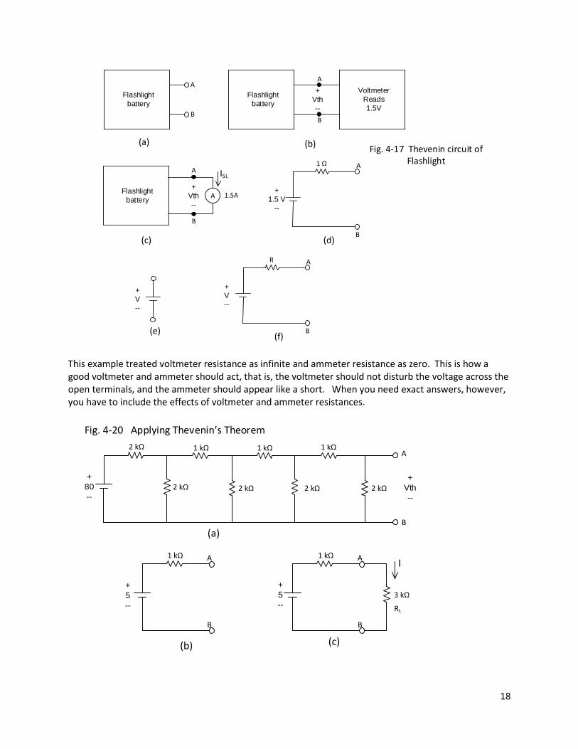
4-16b). When you disconnect the rheostat and measure its resistance (fig. 4-16c), the ohmmeter will read 2 kΩ. In this way, you are finding the Thevenin resistance by measurement rather than calculation. Example 4-11 A flashlight battery is a good example of a sealed box (Fig. 4-17a). When a voltmeter is connected between the terminals, it reads 1.5 V (Fig. 4-17b). When an ammeter is connected between the terminals, it reads 1.5 A (Fig. 4-17c). What is the Thevenin circuit for the flashlight battery? Solution Voltmeters have very high resistances. Because of this, the voltmeter of Fig. 4-17b reads the Thevenin voltage of the battery to a close approximation. As shown in Fig. 4-17b, VTH = 1.5 V. Ammeters have very low resistances. Because of this, the ammeter of Fig. 4-17c reads the shorted-load current to a close approximation. With Eq. (4-3),
RTH =VTH
ISL=
1.5 V
1.5 A= 1Ω
Figure 4-17d shows the Thevenin circuit for a flashlight battery (these are typical values). In earlier discussions, we treated the Thevenin resistance of batteries as zero. This is usually a good approximation because the RTH of the battery is normally much smaller than the load resistances connected to the battery. From now on, whenever we use the symbol of Fig. 4-17e, we mean the source has zero Thevenin resistance. If the Thevenin resistance is important in a discussion or problem, we will draw it separately as shown in Fig. 4-17f.
18
(a)Fig. 4-17 Thevenin circuit of
Flashlight
B
Flashlight
battery
A
(b)
B
Flashlight
battery
A
Voltmeter
Reads
1.5V
+
Vth
--
B
Flashlight
battery
A
+
Vth
--
A
ISL
(c)
+
1.5 V
--
1 A
B(d)
1.5A
+
V
--
+
V
--
R A
B(f)
(e)
This example treated voltmeter resistance as infinite and ammeter resistance as zero. This is how a good voltmeter and ammeter should act, that is, the voltmeter should not disturb the voltage across the open terminals, and the ammeter should appear like a short. When you need exact answers, however, you have to include the effects of voltmeter and ammeter resistances.
2 k
2 k +
80
--
(a)
2 k 2 k 2 k
1 k 1 k 1 k
+
Vth
--
1 k
+
5
--
A
B
A
B
I1 k
+
5
--
A
B
3 k
RL
(b) (c)
Fig. 4-20 Applying Thevenin s Theorem

19
Example 4-14 If you build the circuit of Fig. 4-20a, you will measure a Vth of 5 V. If you also connect a rheostat between the A-B terminals, you will find that a 1-kΩ load resistance drops the voltage to 2.5V. What is the Thevenin circuit to the left of the A-B terminals? Solution This is easy. We are given Vth equal to 5 V. We are also given Rmatch equals 1 kΩ. Therefore, Rth is 1 kΩ. Figure 4-20b summarizes the solution; this is the Thevenin circuit for the original circuit. Example 4-15 If you connect a 3-kΩ load resistance between the A-B terminals of Fig. 4-20a, what is the load current? The load voltage? Solution Figure 4-20c shows the 3-kΩ resistance connected to the Thevenin circuit. The current is
I =5
1000 + 3000= 1.25 mA
and the voltage is
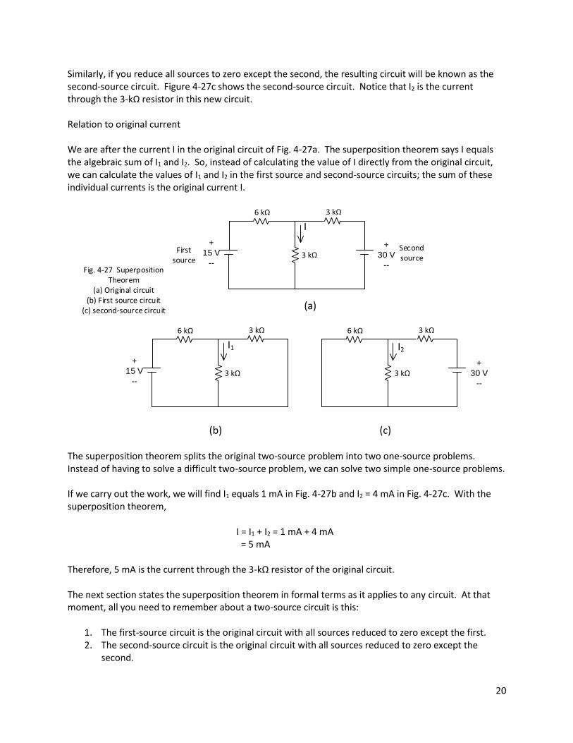
V = RL ∙ I = 3000 × 0.00125 = 3.75 V 4-6 Basic Idea of Superposition Theorem Whenever a circuit has more than one source, the superposition theorem may reduce the work of finding currents and voltages. When you study electronics, you will find the superposition theorem very helpful in understanding how transistor circuits work. This section begins the study of the superposition theorem for a circuit with two sources. In the discussion that follows, dig out the answers to What is a first-source circuit? What is a second-source circuit? How do you apply the superposition theorem? First-source and second-source circuits Figure 4-27a shows a circuit with two voltage sources. To keep the sources distinct, we call the one on the left the first source, and the one on the right the second source. Suppose we are after the current I though the lower 3-kΩ resistor. There are several ways to find the value of I. This section describes the superposition method. The first-source circuit is the new circuit you get when you reduce all sources except the first to zero. Figure 4-27b shows the first-source circuit. I1 is the current through the 3-kΩ resistor in this new circuit.
20
Similarly, if you reduce all sources to zero except the second, the resulting circuit will be known as the second-source circuit. Figure 4-27c shows the second-source circuit. Notice that I2 is the current through the 3-kΩ resistor in this new circuit. Relation to original current We are after the current I in the original circuit of Fig. 4-27a. The superposition theorem says I equals the algebraic sum of I1 and I2. So, instead of calculating the value of I directly from the original circuit, we can calculate the values of I1 and I2 in the first source and second-source circuits; the sum of these individual currents is the original current I.
I
6 k
+
15 V
--3 k
(a)
3 k
+
30 V
--
First source
Second source
I1
6 k
+
15 V
--3 k
(b)
3 k 6 k
3 k
(c)
3 k
+
30 V
--
Fig. 4-27 Superposition Theorem
(a) Original circuit (b) First source circuit
(c) second-source circuit
I2
The superposition theorem splits the original two-source problem into two one-source problems. Instead of having to solve a difficult two-source problem, we can solve two simple one-source problems. If we carry out the work, we will find I1 equals 1 mA in Fig. 4-27b and I2 = 4 mA in Fig. 4-27c. With the superposition theorem,
I = I1 + I2 = 1 mA + 4 mA = 5 mA
Therefore, 5 mA is the current through the 3-kΩ resistor of the original circuit. The next section states the superposition theorem in formal terms as it applies to any circuit. At that moment, all you need to remember about a two-source circuit is this:
1. The first-source circuit is the original circuit with all sources reduced to zero except the first. 2. The second-source circuit is the original circuit with all sources reduced to zero except the
second.

21
Example 4-19 Figure 4-28a shows the equivalent circuit derived in example 4-16. Draw the first-source and second-source circuits.
I
2 k
+
8 V
--
4 k
(a)
2 k
+
4 V
--
I1
2 k
+
8 V
--
4 k
(b)
2 k
I2
2 k 4 k
(c)
2 k
+
4 V
--
Figure 4-28 Example of Superposition
Theorem
Solution When we reduce all sources except the first to zero, we get Fig. 4-28b, the first-source circuit. Note the true direction of I1 must be to the right, because conventional flow is from the positive battery terminal to the negative. To get the second-source circuit, reduce all sources except the second to zero as shown in Fig. 4-28c. Here, the true direction of I2 is to the left because conventional current is from the positive to the negative battery terminal. Example 4-20 Given the circuit of Fig. 4-29a, show the first-source and second-source circuits. Solution Call the upper source the first source, and the lower one the second source. Figure 4-29b is the first-source circuit; Fig. 4-29c is the second-source circuit.
+
6 V
--2 k +
4 V
--
I
(a)
+
6 V
--2 k
I1
(b)
2 k +
4 V
--
(c)
I2
Figure 4-29 Another example of superposition
22
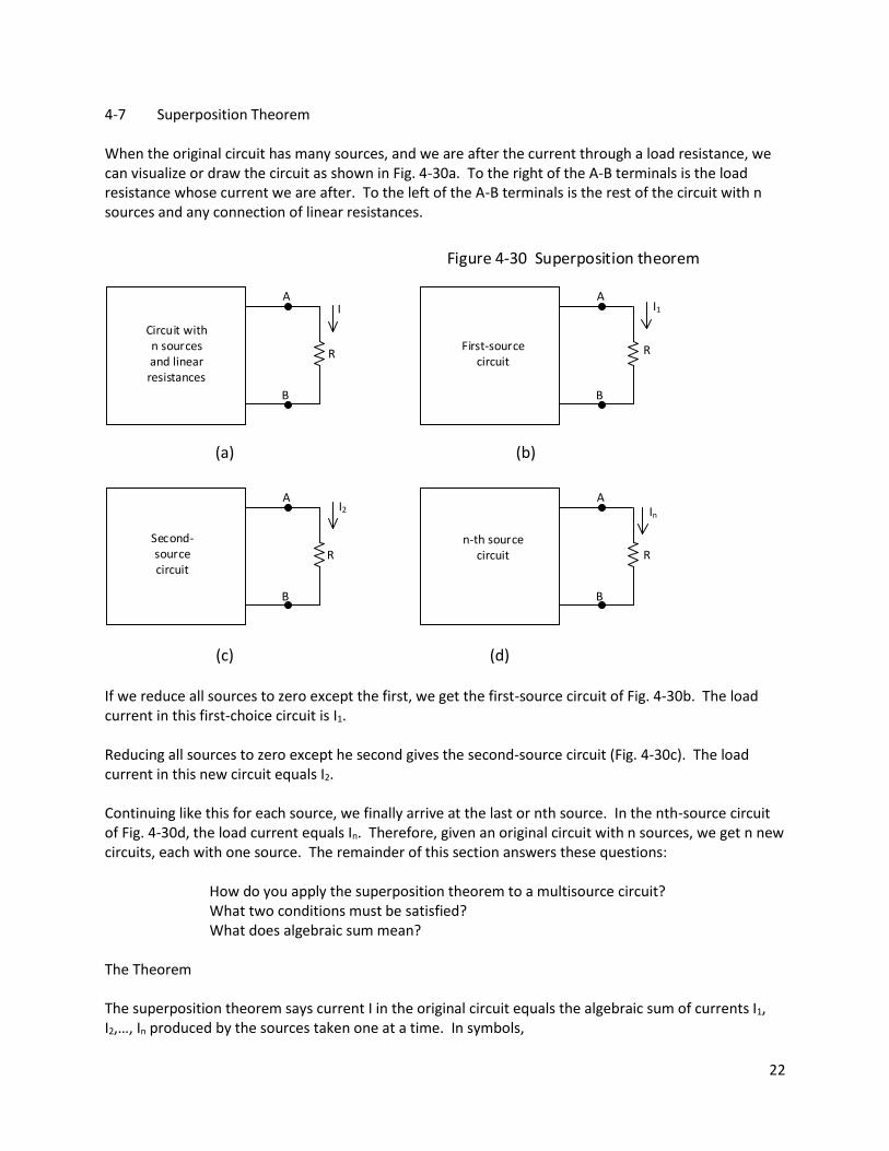
4-7 Superposition Theorem When the original circuit has many sources, and we are after the current through a load resistance, we can visualize or draw the circuit as shown in Fig. 4-30a. To the right of the A-B terminals is the load resistance whose current we are after. To the left of the A-B terminals is the rest of the circuit with n sources and any connection of linear resistances.
Figure 4-30 Superposition theorem
A
B
Circuit with n sources and linear resistances
A
B
A
B
A
B
I I1
First-source circuit
Second-source circuit
n-th source circuit
(a)
R R
R
I2 In
R
(b)
(c) (d) If we reduce all sources to zero except the first, we get the first-source circuit of Fig. 4-30b. The load current in this first-choice circuit is I1. Reducing all sources to zero except he second gives the second-source circuit (Fig. 4-30c). The load current in this new circuit equals I2. Continuing like this for each source, we finally arrive at the last or nth source. In the nth-source circuit of Fig. 4-30d, the load current equals In. Therefore, given an original circuit with n sources, we get n new circuits, each with one source. The remainder of this section answers these questions:
How do you apply the superposition theorem to a multisource circuit? What two conditions must be satisfied? What does algebraic sum mean?
The Theorem The superposition theorem says current I in the original circuit equals the algebraic sum of currents I1, I2,…, In produced by the sources taken one at a time. In symbols,

23
I = I1 + I2 + · · · ·+ In
The superposition theorem reminds us of a divide-and-conquer strategy. We start with an original circuit having n sources. A direct attack means solving for I with all sources in the circuit at the same time. But with the superposition theorem, we divide the original problem into n simpler problems. By solving each simpler problem and summing the individual currents, we get current I in the original circuit. Figure 4-31 summarizes this divide-and-conquer strategy. There are two important conditions that must be satisfied to apply the theorem. They are: All resistances in the circuit including the load must be linear. Otherwise, the superposition theorem is invalid. Also, you can reduce only independent sources to zero. In Eq. 4-10, use the algebraic sum. This means taking the direction of individual currents into account. When an individual current is in the same direction shown for the original current, add the magnitude of the individual current. But when the individual current is opposite the direction shown in the original current, subtract its magnitude.
Figure 4-32 Algebraic summing
A
B
Original circuit
A
B
A
B
I
First-source circuit
Second-source circuit
(a)
R
R
I1 = 5 mA
R
(d)
(b) (c)
(e)
+
V
--
+
V1
--
I2 = 5 mA
+
V2
--
A
B
A
B
First-source circuit
Second-source circuit
R
I1 = 5 mA
R+
V1
--
I2 = 5 mA
+
V2
--

24
Figure 4-32a shows an original circuit with current I down. Suppose the circuit contains two sources. If the first source (Fig. 4-32b) has a downward current of 5 mA and the second-source circuit (Fig 4-32c) has a downward current of 3 mA, the original current is
I = 5 mA + 3 mA = 8 mA On the other hand, if it turns out that I1 is 5 mA downward (Fig. 4-32d) and I2 is 3 mA upward (Fig. 4-32c) then
I = 5 mA - 3 mA = 2 mA I2 opposes or reduces the effect of I1; for this reason, we subtract its magnitude. Voltages We have given the superposition theorem for currents. The same idea applies to voltages. In other words, the voltage across the load resistance in the original circuit equals the algebraic sum of the individual load voltages produced by the sources taken one at a time. In symbols,
V = V1 + V2 + · · · · + Vn
For instance, in Fig. 4-32b, and c, if V1 = 5 V and V2 = 3 V, then V = 8 V. Example 4-21 Calculate the value of I in Fig. 4-33a using the superposition theorem. Check the answer by another method. Solution Figure 4-33b shows the first-source circuit; the current is
I1 = 6
2000= 3 mA
+
6 V
--2 k +
4 V
--
I
(a)
+
6 V
--2 k
I1
(b)
2 k +
4 V
--
(c)
I2
Figure 4-23 Example 4-20
In the second-source circuit of Fig. 4-33c, the current is
I2 = 4
2000= 2 mA
25
Since the individual currents are in the same direction as shown in the original current, add magnitudes to get
I = 3 mA + 2 mA = 5 mA
We can check this answer directly. In Fig. 4-33a, the voltage across the 2-kΩ resistance is the sum of source voltages (Kirchhoff’s voltage law). Therefore, the current equals
I = 10
2000= 5 mA
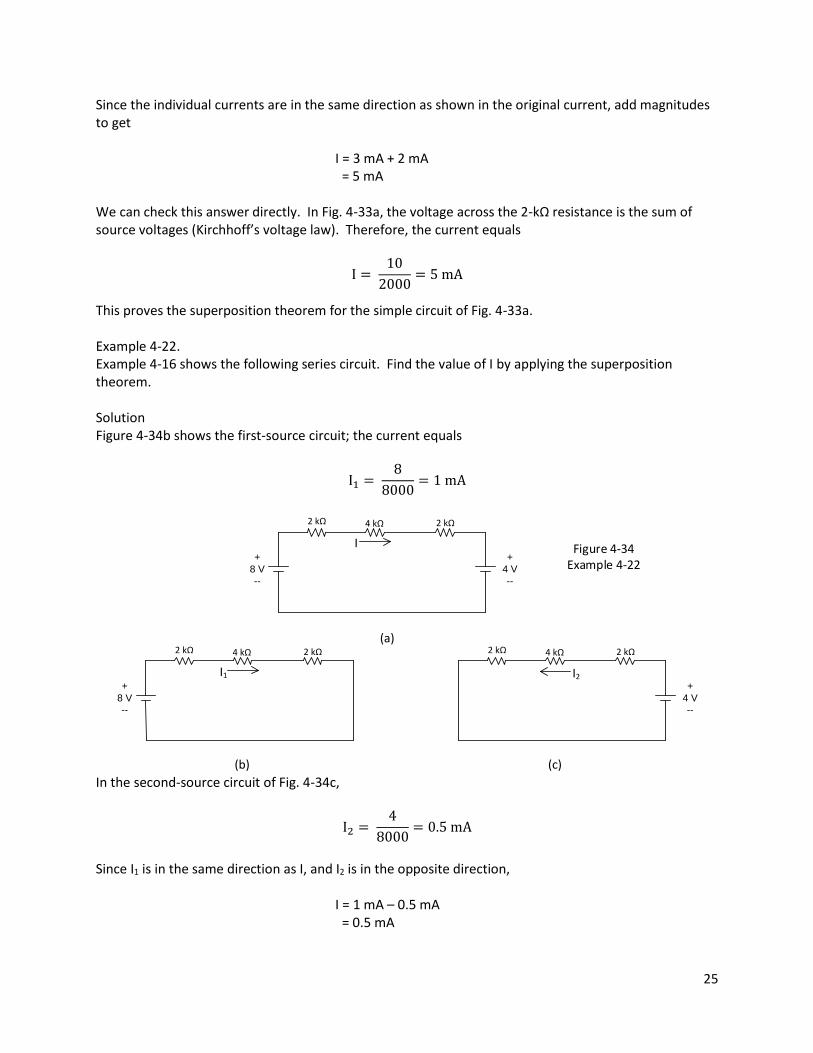
This proves the superposition theorem for the simple circuit of Fig. 4-33a. Example 4-22. Example 4-16 shows the following series circuit. Find the value of I by applying the superposition theorem. Solution Figure 4-34b shows the first-source circuit; the current equals
I1 = 8
8000= 1 mA
I
2 k
+
8 V
--
4 k
(a)
2 k
+
4 V
--
I1
2 k
+
8 V
--
4 k
(b)
2 k
I2
2 k 4 k
(c)
2 k
+
4 V
--
Figure 4-34 Example 4-22
In the second-source circuit of Fig. 4-34c,
I2 = 4
8000= 0.5 mA
Since I1 is in the same direction as I, and I2 is in the opposite direction,
I = 1 mA – 0.5 mA = 0.5 mA

26
This answer found by superposition is the same as the answer found earlier by a different method. Therefore, this proves the superposition theorem for the original circuit of Fig. 4-34a. Example 4-23 Calculate the value of I in Fig. 4-35a.
Figure 4-35 Example 4-23
I
6 k
+
15 V
--3 k
(a)
3 k
+
30 V
--
I1
6 k
+
15 V
--3 k
(b)
3 k
6 k
3 k
(d)
3 k
+
30 V
--
6 k
+
15 V
--
1.5 k
(c)
+
V1
--
2 k
(e)
3 k
+
30 V
--
I2
+
V2
--
Solution Figure 4-35b shows the first-source circuit. Since 3 kΩ are in parallel with 3 kΩ, we get the 1.5 kΩ resistance shown in Fig. 4-35c. With the voltage-divider theorem,
V1 = 1500
6000 + 150015 = 3 V
In Fig. 4-35b, 3 V is across the 3 kΩ resistance; the current through this resistance is
I1 = 3
3000= 1 mA
27
Figure 4-35d shows the second-source circuit; the parallel combination of 6 kΩ and 3 kΩ is the 2 kΩ resistance of Fig. 4-35e. Using the voltage-divider theorem,
V2 = 2000
3000 + 200030 = 12 V
These 12 V are across the middle 3 kΩ resistance of Fig. 4-35d; therefore,
I2 = 12
3000= 4 mA
Currents I1 and I2 are in the same direction as the original current of Fig. 4-35a. So,
I = 1 mA + 4 mA = 5 mA
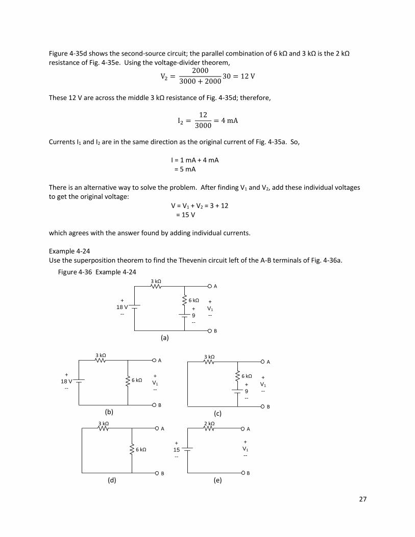
There is an alternative way to solve the problem. After finding V1 and V2, add these individual voltages to get the original voltage: V = V1 + V2 = 3 + 12 = 15 V which agrees with the answer found by adding individual currents. Example 4-24 Use the superposition theorem to find the Thevenin circuit left of the A-B terminals of Fig. 4-36a.
+
V1
--
3 k
+
18 V
--
A
B
6 k
(a)
Figure 4-36 Example 4-24
+
9
--
+
V1
--
3 k
+
18 V
--
A
B
6 k
(b)
+
V1
--
3 k A
B
6 k
(c)
+
9
--
3 k A
B
6 k
(d)
+
V1
--
2 k A
B
(e)
+
15
--

28
Solution This chapter has discussed three theorems: the voltage-divider theorem, Thevenin’s theorem and the superposition theorem. In this example, we use all three theorems. To get the Thevenin circuit for Fig. 36a, we have to work out Vth and Rth. To find Vth, add the voltages produced across the A-B terminals when the sources are taken one at a time. In the first-source circuit of Fig. 4-36b,
V1 = 6000
3000 + 600018 = 12 V
In the second-source circuit of Fig. 4-36c,
V2 = 3000
6000 + 30009 = 3 V
V1 and V2 have the same polarity as Vth; therefore VTH = V1 + V2 = 12 + 3 = 15 V This is the Thevenin voltage for the original circuit. To get RTH, reduce all sources to zero as shown in Fig. 4-36d. The equivalent resistance between the A-B terminals is RTH = 3000 ǁ 6000 Figure 4-36e shows the Thevenin circuit for Fig. 4-36a. Fig. 4-8 Review of the Three Theorems The three theorems of this chapter are among the most practical circuit theorems because they help you solve an enormous range of problems. The voltage-divider theorem is easy to understand and remember. It applies to any one-source series circuit, and says the output voltage across resistance R2 = R2/R times the input voltage. Thevenin’s theorem is outstanding. It reduces a complicated circuit to a series circuit. Because of this, it eliminates all unnecessary information and lets you concentrate on essential part of the problem. The superposition theorem is useful when the original circuit has more than one source. This theorem divides a many-source circuit into simpler one-source circuits.

29
Problems 4-1. In Fig. 4-37a, what is the output voltage when the wiper is all the waya up? All the way down?
At the middle position? 4-2. There are four switch positions in Fig. 4-37b. Calculate the output voltage for each. 4-3. Figure 4-37c shows a step voltage divider used in some voltmeters. What is the value of Vout in
each switch position A through F? 4-4. In the open-load circuit of Fig. 4-38a, what is the vaoue of VTH? RTH? 4-5. Figure 4-38b shows an open-load circuit. What does VTH equal? RTH? 4-6. What is the Thevenin circuit left of the A-B terminals in Fig. 4-38c? 4-7. The wiper of Fig. 4-38d is in the middle of the 20-kΩ potentiometer. What does VTH equal? RTH? 4-8. A 75-kΩ resistance is connected between the A-B terminals of Fig. 4-38a. What is the current
through this resistance? The voltage across it? 4-9. When we connect a 60-kΩ resistance between the A-B terminals of Fig. 4-38b, the voltage
across these terminals decreases. What is the new value of the voltage? 4-10. A 12.5 kΩ resistance is attached to the A-B terminals in Fig. 4-38c. What is the value of the load
current? The load voltage?
Fig. 4-37
+
25 V
--
20 k
(a)
+
15 V
--+
Vout
--
900 k
90 k
10 k
(b)
30 k
+
Vout
--
+
100 V
--
7 M
2 M
700 k
(c)
+
Vout
--
200 k
100 k
A
B
C
D
E
F
4-11. The A-B terminals of Fig. 4-38d are connected to an electronic circuit whose resistance is 10 kΩ:
What is the voltage between the A-B terminals when the wiper is at the middle? At the top? 4-12. In the open-loop circuit of Fig. 4-38e, what does VTH equal? RTH? If a 1-kΩ resistance is
connected between the A-B terminals, what is the current through it? The voltage across it?

30
4-13. A penlight battery has a Thevenin voltage of 1.5 V. When the battery terminals are shorted, the resulting current is 2 A. What is the Thevenin resistance of this battery?
4-14. The battery used in a transistor radio has an open-load voltage of 9 V. When a short is placed between the battery terminals, 1.25 A results. What is the Thevenin resistance of this battery?
20 k
(d)
50 k
50 k +
60 V
--
A
B
30 k
30 k +
20 V
--
A
B
(a)
25 k
(b)
Fig. 4-38
60 k
50 k +
24 V
--
A
B
(c)
2 k
2 k +
4
--
(e)
2 k 2 k 2 k
1 k 1 k 1 k A
B
60 k +
10 V
--A
B
4-15. The voltmeter of Fig. 4-39a has an infinite resistance, and the ammeter of Fig. 4-39b has a zero
resistance. The voltmeter reads 100 mV; the ammeter reads 0.1 mA. What is the Thevenin resistance of the black box?
4-16. In Fig. 4-39a and b, the voltmeter looks like an open and the ammeter like a short. The voltmeter reads 2 V and the ammeter reads 1 mA. If a 3-kΩ resistance is connected between the A-B terminals as shown in Fig. 4-39c, what is the current through it? The voltage across it?
4-17. A black box has an open-load voltage of 10 V and a shorted-load current of 2 mA. If a rheostat is connected between the A-B terminals as shown in Fig. 4-39d, what is the resistance of the rheostat when the load voltage drops to 5 V? What is the resistance if the load voltage equals 7.5 V?
4-20. The open-load voltage of a black box equals 4 V. A load resistance of 8 kΩ results in a load voltage of 2 V. What is the value of the shorted-load current? The through a 32-kΩ load resistance?

31
(a)
Black box
(b)
B
Black box
A
Voltmeter
B
Black box
A
A
(c) (d)
B
Black box
A
A
3 k
B
Figure 4-39
4-21. What is the voltage across the 2-kΩ resistance of Fig. 4-41a? Across the 6 kΩ resistance?
Between the A-B terminals?
(a)
1 k
2 k
3 k
6 k
(b)
(c) (d)
+
48 V
--A B
2 k
1 k
4 k
R
+
24 V
--A B
2 k
4 k
6 k
3 k
+
12 V
--
10 k
30 k
30 k
10 k
+
6 V
-- 6 k
IA
Fig. 4-41
4-22. In Fig. 4-41b, what is the voltage across the 1-kΩ resistance? If R equals 8 kΩ what is the voltage
across R? What value of R balances the bridge? 4-23. Calculate the value of I in Fig. 4-41c.

32
4-24. The ammeter of Fig. 4-41d has such a low resistance that we will approximate it by a zero resistance. What does the ammeter read?
4-25. The tolerance of a resistor is the maximum percent error it can have from its specified value. For instance, a 100-Ω resistor with a tolerance of +/- 5 percent can have a value between 95 Ω and 105 Ω. In Fig. 4-41a, the 1-kΩ resistance has a tolerance of +/- 1 percent. All other resistances have the values shown. What is the maximum voltage that may appear between the A-B terminals?
4-26. Although an ammeter is usually approximated as a zero resistance, it actually has some resistance. Suppose the ammeter of Fig. 4-41d has a resistance of 50 Ω. What is the current through the ammeter? Does the ammeter resistance in this circuit have a small or a large effect on the load current?
4-27. In Fig 4-41b, a short is placed between the A-B terminals. Calculate the current for each of these: a. R = 1 kΩ b. R = 2 kΩ c. R = 3 kΩ
4-28. Draw the first-source and second-source circuits for Fig. 4-42c. 4-29. Draw the first-source, second-source, and third-source circuits of Fig. 4-42d.
4-30. Draw the first-source and second-source circuits of Fig. 4-42e. Do the same for Fig. 4-42f. 4-31. Calculate the value of I in Fig. 4-42a using the superposition theorem. Check the answer by
another method.
Fig. 4-42
+
10 V
--5 k
(a)
+
20 V
--
I
+
10 V
--
5 k
(b)
+
20 V
--
I
12 k
+
72 V
--
6 k
(c)
12 k
+
24 V
--
+
25 V
-- 10 k
(d)
+
5 V
--
I
+
15 V
--
30 k
+
40 V
--
A
B
(e)
10 k
+
20
--
30 k
+
40 V
--
A
B
(f)
10 k
--
20
+
I

33
4-32. What is the value of I in Fig. 4-42b? The value of I1 and I2 in the first-source and second-source circuits?
4-33. Use the superposition theorem to find the value of I in Fig. 4-42c. 4-34. In Fig. 4-42d, work out the value of I with the superposition theorem. What is the voltage across
the 10-kΩ resistance? 4-35. Work out the Thevenin voltage across the A-B terminals of Fig. 4-42e by using the superposition
theorem. 4-36. The 20-V source of Fig. 4-42f has the opposite polarity from the 20-V source of Fig. 4-42e. What
is the Thevenin voltage between the A-B terminals of Fig. 4-42e? Of Fig. 4-42f? 4-37. A 12.5 kΩ resistance is connected between the A-B terminals of Fig. 4-42e. What is the current
through this resistance? The voltage across it?