1

4.13-aGCOM-C/SGLI progress

Hiroshi Murakami

Earth Observation Research Center,

Japan Aerospace Exploration Agency

IOCCG#15 Jan. 19 2009

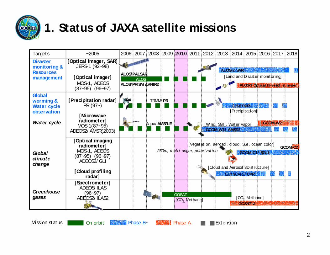
Targets ~2005 2006 2007 2008 2009 2010 2011 2012 2013 2014 2015 2016 2017 2018

Disaster monitoring & Resources management

[Optical imager, SAR]JERS-1 (92~98)

[Optical imager]MOS-1, ADEOS

(87~95) (96~97)Global worming & Water cycle observation

Water cycle

[Precipitation radar]PR (97~)

[Microwave radiometer]MOS-1(87~95)

ADEOS2/AMSR(2003)

Global climate change

[Optical imaging radiometer]

MOS-1, ADEOS(87~95) (96~97)

ADEOS2/GLI

[Cloud profiling radar]

Greenhouse gases

[Spectrometer]ADEOS/ILAS

(96~97)ADEOS2/ILAS2

2

Phase AOn orbit ExtensionMission status

[Land and Disaster monitoring]

GPM/DPR

Aqua/AMSR-E

GCOM-C1/ SGLI

[Vegetation, aerosol, cloud, SST, ocean color]

[Cloud and Aerosol 3D structure]

GOSAT[CO2, Methane]

TRMM/PR

GCOM-W1/ AMSR2[Wind, SST , Water vapor]

Phase B~

[Precipitation]

[CO2, Methane]

GCOM-W2

GOSAT-2

ALOS-3 Optical hi-resol. & hyper

ALOS-2 SARALOS/PALSAR

ALOS/PRISM AVNIR2ALOS

EarthCARE/CPR

250m, multi-angle, polarizationGCOM-C2

1. Status of JAXA satellite missions

3

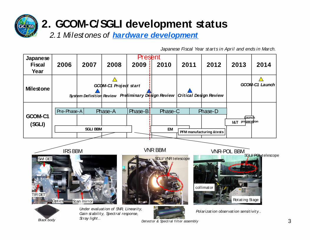
2. GCOM-C/SGLI development status2.1 Milestones of hardware development

Japanese Fiscal Year

2006 2007 2008 2009 2010 2011 2012 2013 2014

Milestone

GCOM-C1(SGLI)

Present

Phase-B Phase-CPhase-A Phase-D

GCOM-C1 Launch

Pre-Phase-A

Preliminary Design Review Critical Design ReviewSystem Definition Review

GCOM-C1 Project start

Japanese Fiscal Year starts in April and ends in March.

SGLI BBM EMPFM manufacturing &tests

Optics

SWI DET

TIR DET

Scan mirror

IRS BBM VNR BBM

Under evaluation of SNR, Linearity,Gain stability, Spectral response, Stray light..

I&TLaunch

preparation

collimator

Rotating Stage

VNR-POL BBM

Polarization observation sensitivity..

SGLI/POL telescopeSGLI/VNR telescope

Black body Detector & Spectral filter assembly

4

Japanese Fiscal Year Apr~ 2008 2009 2010 2011 2012 2013 2014 2015 2016 2017 2018 2019

Sensor development &

calibration

1. Design and trial manufacturing

2. Sensor manufacturing & tests 3. Initial calibration

4. Operation phase

Research Announcement RA#1 RA#2 RA#3

Product version ups & Software implementation

Algorithm development & improvement •Preparation

study•Investigation of candidates

•Theoretical performance and applicability

•Selection & development of operational algorithm

•Product validation and improvement•Achievement of GCOM-C science targets•New algorithm and usage•Succession to the GCOM-C2

BBM EMPFM

Phase-B Phase-C Phase-D

Inplementation-1Performance test

Imple. -2Operation test

Intensive Cal/Val phase

Improvement with product version up

Implement for C2

Version-ups & improvement

1. Initial development

2.Performance development

3. Operational algorithm

4. Post-launch development and improvement phase

GCOM-C1

LaunchGCOM-C2

GCOM-C3

Analysis usingexisting satellite data

Project start

System PDR

System CDR

GCOM-C1 launch Data Release

C2 Launch

Mission result evaluation

5 years~13 years

Development of algorithm performance and operational code

Selection

Phase-A

Ver.1 Ver.0 Ver.2 Ver.2.5 Ver.3for C-1&2

2. GCOM-C/SGLI development status2.2 Milestones of Product development

Area PI name Organization

Land

Y. Honda (land reflectance val) Chiba Univ.

K. Nasahara (NPP, LAI, Flux..) Tsukuba Univ.

K. Kajiwara (biomass by BRF) Chiba Univ.

Q-X. Wang (evapotranspiration) NIES

A. Ono (water stress, shadow index) JAXA/EORC

S. Furuumi (UPDM index) Narasaho college

K. Fukue (land cover) Tokai Univ.

N. Soyama (land cover) Tenri Univ.

M. Moriyama (LST, fire detection) Nagasaki Univ.

M. Tasumi (Crop Coefficient) Miyazaki Univ.

K. Ichii (model) Fukushima Univ.

T. Kaneko (volcano) Tokyo Univ. ERI

R. Suzuki (LAI, time series) JAMSTEC

A. Huete (Vegetation index) The University of Arizona

T. Miura (Vegetation time series) University of Hawaii at Manoa

M. Takagi (local land cover, GCP) Kochi Univ. of Technology

K. Mabuchi (model) Meteorological Research Institute

K. Nakau (fire detect., burned area) JAXA/EORC

Area PI name Organization

Atmosphere

Takashi Nakajima (cloud) Tokai Univ.

M. Kuji (Cloud thickness) Nara Women's Univ.

N. Schutgens (aerosol, SKYNET) Tokyo Univ.

I. Sano (Pol aerosol, Atm Corr.) Kinki Univ

Y. Mano (non spherical) Meteorological Research Institute

J. Riedi (Pol cloud) LOV, Lille UnivO

cean

M. Toratani (Atmos. Corr) Tokai Univ.

R. Frouin (Atmos. Corr. function) Scripps Institution of Oceanography

T. Hirawake (NPP/PFT) Hokkaido Univ.

T. Hirata (IOP, PFT, model) Plymouth Marine Laboratory

J. Ishizaka (redtide) Nagoya Univ.

F. Sakaida (SST) Tohoku Univ.

S. Saitoh (fishery) Hokkaido Univ.

H. Kawamura (coastal monitoring) Tohoku Univ.

T. Iida (polar area biology) National Institute of Polar Research

Criosphere

T. Aoki (snow size impurity) Meteorological Research Institute

K. Stamnes (snow size temperature) Stevens Institute of Technology

5

• The first research opportunity for GCOM-C was announced in January 2009

• The science team, including international participation, has been organized in July 2009 (35 Principal Investigators including 6 foreign PIs from US, France, and UK).

• Algorithm development, in-situ data acquisition, and application research using other satellite data are conducted by collaboration among JAXA/EORC and the PI members

2. GCOM-C/SGLI development status2.3 GCOM-C Principal Investigators

Red: PI team leaderBlue: Group leaders

6

• Sensor operation Regular yearly pattern will be prepared considering intensive areas and seasonality before launch Irregular tilt angles of polarimetry, 1km/250m resolution, and calibration modes will be planned

more than three months before the operation All data will be received at the Svalbard station; near-real time data at a station in Japan

• Free of charge for internet acquisition The standard products (including Levels 1, 2 and 3) will be distributed with free of charge from

EORC information system which is a common system for several other missions (Search & download, and FTP directory: TBD)

Re-distribution by users is limited to pre-defined users (to identify users by JAXA)

SGLI basic operation* modesBasic modes VN1‐8,10‐11 VN9, SW1‐2 SW3 SW4 T1‐2 P1‐2

Day‐land/coast 250m 1km 250m  1km500m

1km +45

250m** 45

Day‐offshore/polar 1km 1km 1km 1km 1km 1km +4545

Night‐land OFF OFF 250m 1km500m

OFF250m**

Night‐coast OFF OFF OFF OFF500m

OFF250m**

Night‐offshore/polar OFF OFF OFF OFF 1km OFF

*: Other modes for cal/val and special requests will be planned more than three months before the operation**:  250m mode is limited by downlink data volume per a path

2. GCOM-C/SGLI development status2.4 Sensor operation and data distribution policy

Band cVN1 380nmVN2 412nmVN3 443nmVN4 490nmVN5 530nmVN6 565nmVN7 673.5nmVN8 673.5nmVN9 763nmVN10 868.5nmVN11 868.5nm

P1 673.5nmP2 868.5nm

SW1 1050nmSW2 1380nmSW3 1630nmSW4 2210nmT1 10.8umT2 12.0um

7

3. Summary• GCOM-C targets

• Improvement of knowledge and future prediction of the climate system through long-term observations regarding radiation budget and carbon cycle

• GCOM-C/SGLI characteristics• 250-m resolution and 1150-km swath for the land and coast observations• Near-UV and polarization observation for the land aerosol estimation• Multi-angle observation for the biomass and land cover classification

• Schedule• Satellite, sensor (finished the first component studies), and algorithm are developing

for the launch in 2014• Governmental mission evaluation has been done (Nov.-Dec. 2009), but..• GCOM-C PI team (2009-2012) has organized in summer 2009 through the first research

announcement• The first PI workshop was held in Tokyo Jan. 12-14 2010

• Science challenges• Integrated use of GCOM-C and other data (in-situ and other satellites) for the global

estimation and model improvement• Optical connection between satellite and (bio/)physical parameters for the optimum

use of the multi-spectral, multi-angle, and polarization observations• Others• International collaboration (JAXA-CNES, GCOM-NOAA..) are discussed

8

Backup

9

Solar calibration window

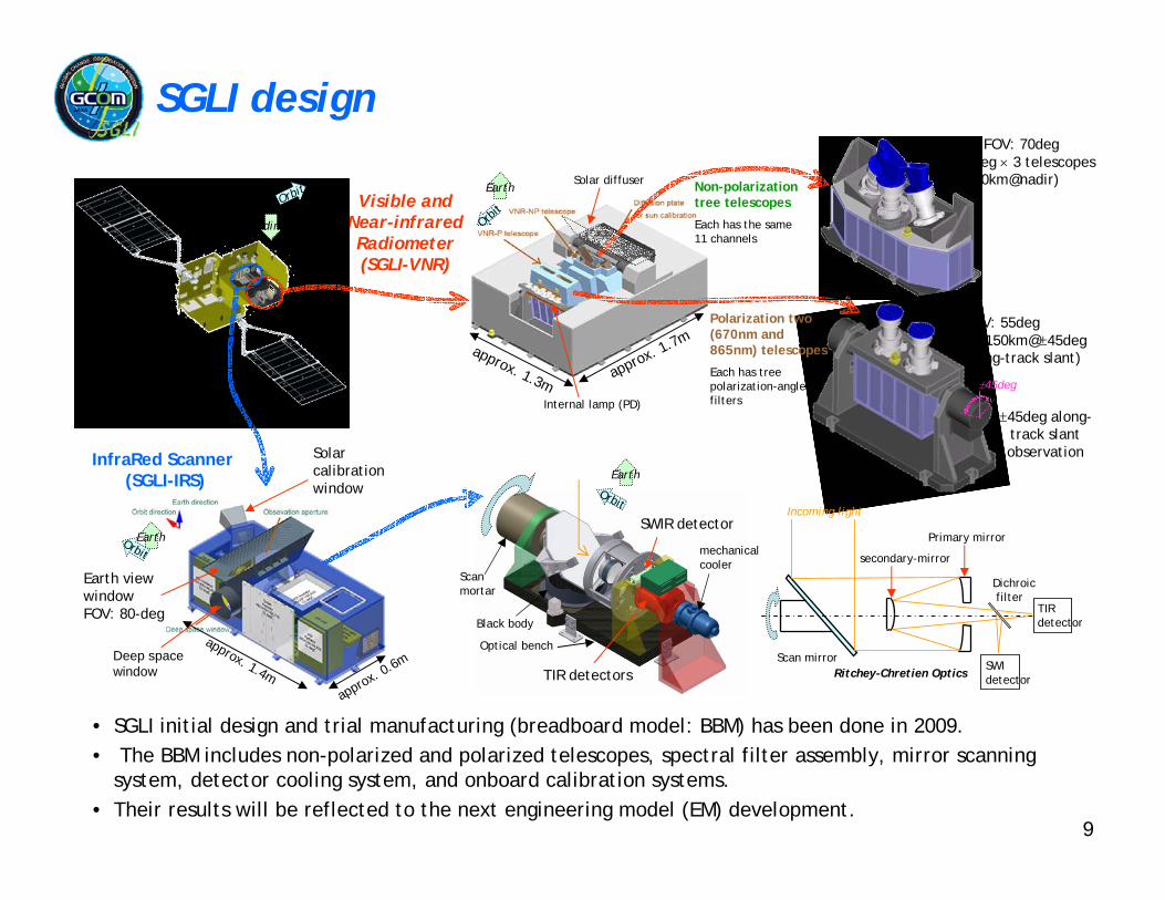
Earth view windowFOV: 80-deg

Deep space window

approx. 1.4m

approx. 0.6m

Visible and Near-infraredRadiometer(SGLI-VNR)

Non-polarization tree telescopes

Each has the same 11 channels

Solar diffuser

approx. 1.7m

approx. 1.3m

GCOM-Csatellite

Total FOV: 70deg = 24deg 3 telescopes(~1150km@nadir)

Earth direction

Earth

Earth

45deg along-track slant observation

Polarization two (670nm and 865nm) telescopes

Each has tree polarization-angle filters

Scan mortar

Black body

SWIR detector

TIR detectors

Optical bench

Earth

mechanical cooler

Dichroicfilter

TIR detector

SWI detector

Primary mirror

secondary-mirror

Ritchey-Chretien Optics Scan mirror

Incoming light

FOV: 55deg(~1150km@45deg along-track slant)

Orbit

Orbit

Orbit

Orbit

InfraRed Scanner (SGLI-IRS)

45deg

SGLI design

Internal lamp (PD)

• SGLI initial design and trial manufacturing (breadboard model: BBM) has been done in 2009.• The BBM includes non-polarized and polarized telescopes, spectral filter assembly, mirror scanning

system, detector cooling system, and onboard calibration systems. • Their results will be reflected to the next engineering model (EM) development.

10

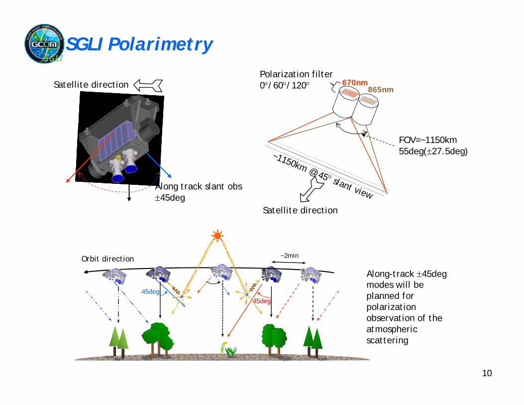
Along-track 45deg modes will be planned for polarization observation of the atmospheric scattering

SGLI Polarimetry

Along track slant obs45deg

Satellite directionPolarization filter0/60/120

Satellite direction

670nm865nm

FOV=~1150km55deg(27.5deg)~1150km @ 45 slant view

Orbit direction

45deg

~2min

45deg

11

SGLI channels

CH

Lstd Lmax SNR at Lstd IFOV

VN, P, SW: nmT: m

VN, P: W/m2/sr/m

T: Kelvin

VN, P, SW: -T: NET

m

VN1 380 10 60 210 250 250VN2 412 10 75 250 400 250VN3 443 10 64 400 300 250VN4 490 10 53 120 400 250VN5 530 20 41 350 250 250VN6 565 20 33 90 400 250VN7 673.5 20 23 62 400 250VN8 673.5 20 25 210 250 250VN9 763 12 40 350 1200 1000VN10 868.5 20 8 30 400 250VN11 868.5 20 30 300 200 250P1 673.5 20 25 250 250 1000P2 868.5 20 30 300 250 1000

SW1 1050 20 57 248 500 1000SW2 1380 20 8 103 150 1000SW3 1630 200 3 50 57 250SW4 2210 50 1.9 20 211 1000T1 10.8 0.7 300 340 0.2 500T2 12.0 0.7 300 340 0.2 500

• The SGLI features are finer spatial resolution (250m (VNI) and 500m (T)) and polarization/along-track slant view channels (P), which will improve land, coastal, and aerosol observations.

GCOM-C SGLI characteristics (Current baseline)

OrbitSun-synchronous (descending local time: 10:30)Altitude: 798km, Inclination: 98.6deg

Launch Date Jan. 2014 (HII-A)Mission Life 5 years (3 satellites; total 13 years)

ScanPush-broom electric scan (VNR: VN & P)Wisk-broom mechanical scan (IRS: SW & T)

Scan width1150km cross track (VNR: VN & P)1400km cross track (IRS: SW & T)

Digitalization 12bitPolarization 3 polarization angles for PAlong track direction

Nadir for VN, SW and T, +45 deg and -45 deg for P

On-board calibration

VN: Solar diffuser, Internal lamp (PD), Lunar by pitch maneuvers, and dark current by masked pixels and nighttime obs.

SW: Solar diffuser, Internal lamp, Lunar, and dark current by deep space window

T: Black body and dark current by deep space window

All: Electric calibration

Multi-angle obs. for 674nm and 869nm

GCOM-C development statusSatellite orbit and SGLI specification

250m over the Land or coastal area, and 1km over offshore

250m-mode possibility ~15min /path (TBC)

12

Land

Surface reflectance

Precise geometric correction both 250m <1pixel*6 <0.5pixel*6 <0.25pixel*6

Atmospheric corrected reflectance (incl. cloud detection)

Daytime

250m 0.3 (<=443nm), 0.2 (>443nm) (scene) *7

0.1 (<=443nm), 0.05 (>443nm) (scene) *7

0.05 (<=443nm), 0.025 (>443nm) (scene)*7

Vegetation and carbon cycle

Vegetation index 250m Grass:25%(scene), forest:20%(scene)

Grass:20%(scene), forest:15%(scene)

Grass:10%(scene), forest:10%(scene)

Above-ground biomass 1km Grass:50%, forest: 100% Grass:30%, forest:50% Grass:10%, forest:20%

Vegetation roughness index 1km Grass&forest: 40% (scene) Grass& forest:20% (scene) Grass&forest:10% (scene)

Shadow index 250m, 1km Grass&forest: 30% (scene) Grass& forest:20% (scene) Grass&forest:10% (scene)

fAPAR 250m Grass:50%, forest: 50% Grass:30%, forest:20% Grass:20%, forest:10%

Leaf area index 250m Grass:50%, forest: 50% Grass:30%, forest:30% Grass:20%, forest:20%

temperature Surface temperature Both 500m <3.0K (scene) <2.5K (scene) <1.5K (scene)

Common note:*1: The “release threshold” is minimum levels for the first data release at one year from launch. The "standard" and "research" accuracies

correspond to full- and extra success criteria of the mission respectively. Accuracies are shown by RMSE basically.

Radiance data note:*2: TOA radiance is derived from sensor output with the sensor characteristics, and other products are physical parameters estimated using

algorithms including knowledge of physical, biological and optical processes *3: absolute error is defined as offset + noise*4: relative error is defined as relative errors among channels, FOV, and so on. *5: Release threshold of radiance is defined as estimated errors from vicarious, onboard solar diffuser, and onboard blackbody calibration because

of lack of long-term moon samples

Land data note:*6: Defined as RMSD from GCP*7: Defined with land reflectance~0.2, solar zenith<30deg, and flat surface. Release threshold is defined with AOT@500nm<0.25

GCOM-C products (1/3)GCOM-C products accuracy targets (Standard-1)

Area group Product Day/night Grid size Release threshold*1 Standard accuracy*1 Target accuracy*1

Comm

on

radiance

TOA radiance(including system geometric correction)

TIR and land 2.2m: both

Other VNR,SWI: daytime (+special operation)

VNR,SWILand/coast: 250m, offshore: 1km, polarimetory:1kmTIRLand/coast: 500m, offshore: 1km

Radiometric 5% (absolute*3)*5

Geometric<1pixel

VNR,SWI: 5% (absolute*3), 1% (relative*4)

TIR: 0.5K (@300K)Geometric<0.5pixel

VNR,SWI: 3% (absolute*3), 0.5% (relative*4)

TIR: 0.5K (@300K) Geometric<0.3pixel

13

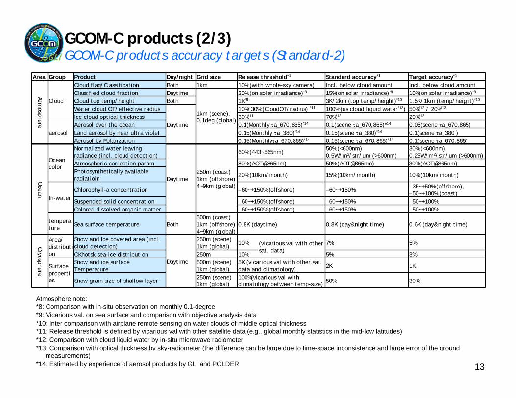
Area Group Product Day/night Grid size Release threshold*1 Standard accuracy*1 Target accuracy*1

Atmosphere

Cloud

Cloud flag/Classification Both 1km 10% (with whole-sky camera) Incl. below cloud amount Incl. below cloud amountClassified cloud fraction Daytime

1km (scene),0.1deg (global)

20% (on solar irradiance)*8 15%(on solar irradiance)*8 10%(on solar irradiance)*8

Cloud top temp/height Both 1K*9 3K/2km (top temp/height)*10 1.5K/1km (temp/height)*10

Water cloud OT/effective radius

Daytime

10%/30% (CloudOT/radius) *11 100% (as cloud liquid water*13) 50%*12 / 20%*13

Ice cloud optical thickness 30%*11 70%*13 20%*13

aerosolAerosol over the ocean 0.1(Monthly a_670,865)*14 0.1(scene a_670,865)*14 0.05(scene a_670,865)Land aerosol by near ultra violet 0.15(Monthly a_380)*14 0.15(scene a_380)*14 0.1(scene a_380 )Aerosol by Polarization 0.15(Monthlya_670,865)*14 0.15(scene a_670,865)*14 0.1(scene a_670,865)

Ocean

Ocean color

Normalized water leaving radiance (incl. cloud detection)

Daytime250m (coast)1km (offshore)4~9km (global)

60% (443~565nm) 50% (<600nm)0.5W/m2/str/um (>600nm)

30% (<600nm)0.25W/m2/str/um (>600nm)

Atmospheric correction param 80% (AOT@865nm) 50% (AOT@865nm) 30% (AOT@865nm)Photosynthetically available radiatioin 20% (10km/month) 15% (10km/month) 10% (10km/month)

In-waterChlorophyll-a concentration 60~+150% (offshore) 60~+150% 35~+50% (offshore),

50~+100% (coast)Suspended solid concentration 60~+150% (offshore) 60~+150% 50~+100%Colored dissolved organic matter 60~+150% (offshore) 60~+150% 50~+100%

temperature Sea surface temperature Both

500m (coast)1km (offshore)4~9km (global)

0.8K (daytime) 0.8K (day&night time) 0.6K (day&night time)

Cryosphere

Area/ distribution

Snow and Ice covered area (incl. cloud detection)

Daytime

250m (scene) 1km (global) 10% (vicarious val with other

sat. data)7% 5%

OKhotsk sea-ice distribution 250m 10% 5% 3%

Surface properties

Snow and ice surface Temperature

500m (scene) 1km (global)

5K (vicarious val with other sat. data and climatology) 2K 1K

Snow grain size of shallow layer 250m (scene) 1km (global)

100%(vicarious val with climatology between temp-size) 50% 30%

Atmosphere note:*8: Comparison with in-situ observation on monthly 0.1-degree*9: Vicarious val. on sea surface and comparison with objective analysis data*10: Inter comparison with airplane remote sensing on water clouds of middle optical thickness*11: Release threshold is defined by vicarious val with other satellite data (e.g., global monthly statistics in the mid-low latitudes)*12: Comparison with cloud liquid water by in-situ microwave radiometer*13: Comparison with optical thickness by sky-radiometer (the difference can be large due to time-space inconsistence and large error of the ground

measurements)*14: Estimated by experience of aerosol products by GLI and POLDER

GCOM-C products (2/3)GCOM-C products accuracy targets (Standard-2)

14

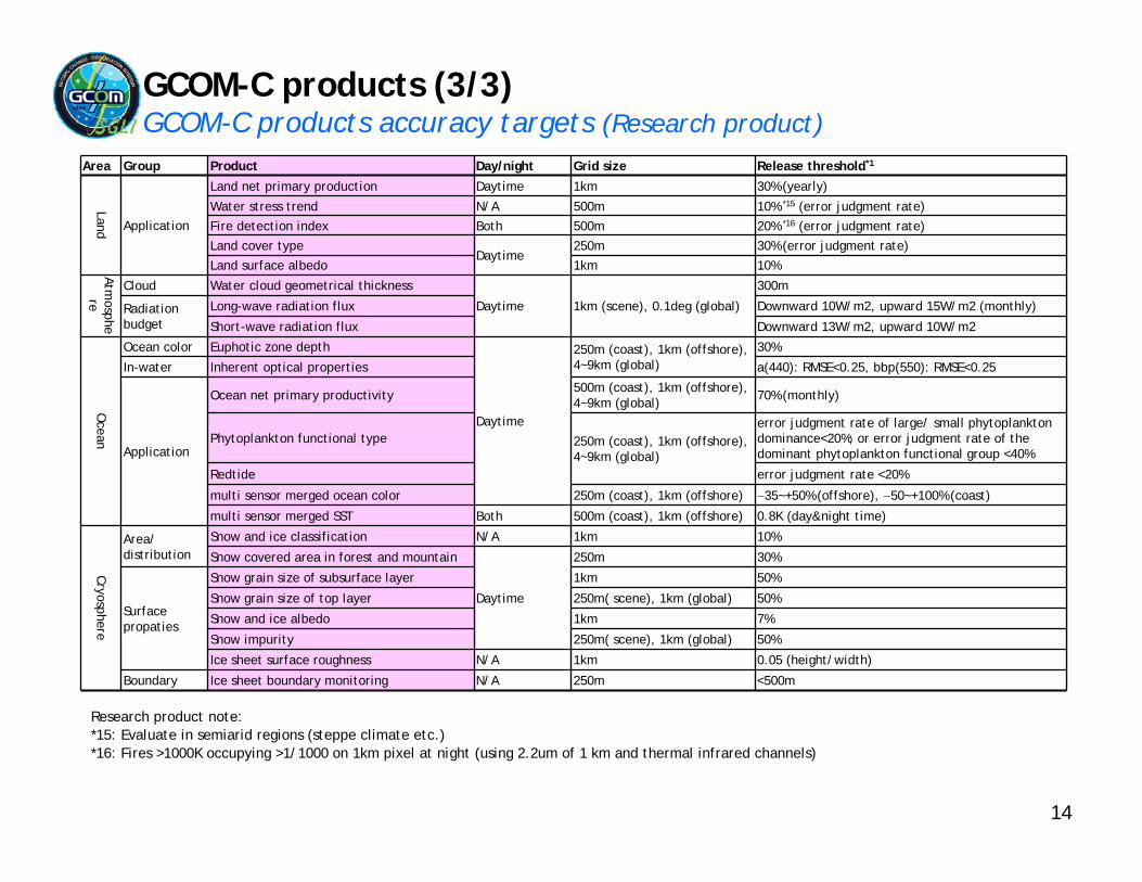
Research product note:*15: Evaluate in semiarid regions (steppe climate etc.)*16: Fires >1000K occupying >1/1000 on 1km pixel at night (using 2.2um of 1 km and thermal infrared channels)

Area Group Product Day/night Grid size Release threshold*1

Land Application

Land net primary production Daytime 1km 30% (yearly)

Water stress trend N/A 500m 10% *15 (error judgment rate)

Fire detection index Both 500m 20% *16 (error judgment rate)

Land cover typeDaytime

250m 30% (error judgment rate)

Land surface albedo 1km 10%Atmosphere

Cloud Water cloud geometrical thickness

Daytime 1km (scene), 0.1deg (global)

300m

Radiation budget

Long-wave radiation flux Downward 10W/m2, upward 15W/m2 (monthly)

Short-wave radiation flux Downward 13W/m2, upward 10W/m2

Ocean

Ocean color Euphotic zone depth

Daytime

250m (coast), 1km (offshore), 4~9km (global)

30%

In-water Inherent optical properties a(440): RMSE<0.25, bbp(550): RMSE<0.25

Application

Ocean net primary productivity 500m (coast), 1km (offshore), 4~9km (global) 70% (monthly)

Phytoplankton functional type 250m (coast), 1km (offshore), 4~9km (global)

error judgment rate of large/ small phytoplankton dominance<20%; or error judgment rate of the dominant phytoplankton functional group <40%

Redtide error judgment rate <20%

multi sensor merged ocean color 250m (coast), 1km (offshore) 35~+50% (offshore), 50~+100% (coast)

multi sensor merged SST Both 500m (coast), 1km (offshore) 0.8K (day&night time)

Cryosphere

Area/ distribution

Snow and ice classification N/A 1km 10%

Snow covered area in forest and mountain

Daytime

250m 30%

Surface propaties

Snow grain size of subsurface layer 1km 50%

Snow grain size of top layer 250m( scene), 1km (global) 50%

Snow and ice albedo 1km 7%

Snow impurity 250m( scene), 1km (global) 50%

Ice sheet surface roughness N/A 1km 0.05 (height/width)

Boundary Ice sheet boundary monitoring N/A 250m <500m

GCOM-C products (3/3)GCOM-C products accuracy targets (Research product)