46 - california institute of technology

Chapter 4

Point Estimation

Frank Porter May 2, 2018

A major theme in statistics is what we call data reduction. We may haveacquired data in a highly multi-dimensional sample space, but are interested inanswering questions of low dimensionality. For example, we may be interested inwhether CP violation in the decay B → JψK0

S is consistent with the constraintsof the Cabibbo-Kobayshi-Maskawa matrix description in the standard model.To answer this question may require looking at the results of 100 million particlecollision events or more, where each event involves the recording of order 104

datums from the apparatus. That is a lot of random variables to answer aone-dimensional question.

In this example, we take the measured data for each event (largely pulseheights and times from different elements of the detector) and turn it into moreintuitive information, such as momenta, directions, energy deposits, and parti-cle types. This reduces the information in a single event from 104 to order 102

dimensions. This information may then be used to decide whether the event isof interest to the question or not. If not, it is dropped from the remaining anal-ysis. The data in the events that pass this selection are then used to addressthe question at hand. This is done by forming some function of the randomvariables for each event that contains the relevant information, and then com-bining the information from all of the events. In this way, our many-dimensionalsample space is reduced to one or a few dimensions. This is the process of datareduction.

Experiments are generally expensive, both in money and time. So, we wantthis data reduction process to make effective use of our resources. For example,we would prefer not to waste relevant information as we reduce the data. We’llintroduce a variety of criteria for “effectiveness” in our discussion of “pointestimation” in this chapter.

47

48 CHAPTER 4. POINT ESTIMATION

4.1 Parametric Statistics

Making a measurement corresponds to taking a sample from some probabilitydistribution, or sampling distribution. The goal of the measurement process isto learn something about this distribution.

Often we know (or assume) something about the form of the sampling dis-tribution. For example, we may know that the mean of the distribution is aquantity of physical interest. In this case, the sampling gives a direct estimateof the quantity we are interested in. We say “estimate” because of the fluctu-ations – any given measurement will typically have some deviation, or error,from the correct value. The quantity of interest is a parameter of the dis-tribution. The branch of statistics that deals with estimation of parameters ofdistributions is called parametric statistics.

It may also happen that we do not know, or do not wish to assume, anythingabout the form of the sampling distribution. It may be the distribution itselfthat we are trying to measure, for example a spectrum. In such a case, we aredealing with non-parameteric statistics. We will concentrate on parametricstatistics for now, returning to the non-parametric case in later chapters.

We will develop the subject of hypothesis testing in a later chapter. However,it is a ubiquitous concept, and it is useful to introduce the concept in the presentcontext. We may regard each guess for the true sampling distribution as ahypothesis. In the context of parameteric statistics, the possible points inparameter space correspond to hypotheses. That is, the parameter space is thespace of possible hypotheses.

We suppose that θ is a physically-interesting parameter, or possibly a vectorof parameters. In parametric statistics, we assume that the sampling distribu-tion (PDF) is of the form:

f(x) = f(x; θ), (4.1)

where f is a function of x and θ known to whatever level we require in ourdiscussion. Our goal is to estimate θ. This is the problem of Point Estimation.We’ll introduce the notation of a “hat” accent mark to indicate an estimator.For example, θ is an estimator for the unknown parameter θ. An estimator is afunction of our sampled data θ = θ(x), thus an estimator is a random variablewith its own sampling distribution, derived from the sampling distribution forx.

A particularly simple form of parameterization is a location parameter:

Definition 4.1 If the probability density function is of the form:

f(x; θ) = f(x− θ),

then θ is called a location parameter for x.

If f(x) is plotted as a function of x, then changes in θ will shift f(x) by anamount equal to the change in θ, but the shape of the function is not changed.For example, in the normal distribution:

f(x) =1

2πexp

[− (x− θ)2

2

],

4.1. PARAMETRIC STATISTICS 49

θ is a location parameter for random variable X.Of course, we would like to get the best estimate possible with the data

we have. Defining what “best” means, however, is not entirely straightforward.There are several properties we might wish to have in defining what we meanby best:

• An unbiased estimator is one that “gets it right on the average”:

Definition 4.2 The bias, b, of an estimator θ for θ is

b(θ) ≡ 〈θ〉 − θ. (4.2)

Note that the bias is in general a function of θ. An unbiased estimatoris one for which b = 0, independent of θ.

Given a biased estimator, it is sometimes possible to modify it to “correct”for the bias and obtain an unbiased estimator. Note that bias is oftenthought of as a “systematic error”, particularly when we know a bias mayexist but don’t attempt to correct for it.

Example: Given an IID sample of size n from some distribution withfinite variance s, we wish to use our data to estimate s. Consider thesample variance (There are differing definitions of sample variance, in-cluding the quantity s′ in Eq. 4.7. We’ll adopt the definition given here,but the possible confusion can be avoided by the description “sample sec-ond central moment”.):

s =1

n

n∑i=1

(xi −m)2, (4.3)

where m is the sample mean, m = 1n

∑ni=1 xi.

We compute the bias of the sample variance as an estimator for s. We’llshow this in detail, as an instructive sample of such computations. Let θbe the mean of the distribution.

b(s) = 〈s〉 − s

= 〈 1n

n∑i=1

(xi −m)2〉 − s

=1

n

n∑i=1

〈(xi −m)2〉 − s

= 〈(x1 −m)2〉 − s, since IID

= 〈(x1 − θ + θ −m)2〉 − s= 〈(x1 − θ)2〉+ 〈(θ −m)2〉+ 2〈(x1 − θ)(θ −m)〉 − s

= s+ 〈

[1

n

n∑i=1

(θ − xi)

]2〉+ 2〈(x1 − θ)(θ −

x1n− 1

n

n∑i=2

xi)〉 − s


=1

n2

n∑i=1

〈(θ − xi)2〉+2

n2

∑i<j

〈(θ − xi)(θ − xj)〉

+2

n〈(x1 − θ)(θ − x1)〉+ 2〈(x1 − θ)

1

n

n∑i=2

(θ − xi)〉

=s

n− 2s

n+ 2〈(x1 − θ)〉〈(

1

n

n∑i=2

xi)〉, since independent

=s

n− 2s

n. (4.4)

(4.5)

Thus, the bias of this estimator is − sn .

In this case, we can make a simple modification to obtain an unbiasedestimator for s. We note that

〈s〉 = s

(1− 1

n

). (4.6)

This, we will have an unbiased estimator for s if we simply multiply s byn/(n− 1). That is,

s′ =1

n− 1

n∑i=1

(xi −m)2 (4.7)

is an unbiased estimator for the variance.

• A consistent estimator gets it right for large statistics:

Definition 4.3 An estimator, θ, is consistent if

limn→∞

θ(x1, x2, . . . , xn) = θ. (4.8)

That is, an estimator is consistent if it converges to the parameter in thelimit of large statistics.

Note the distinction between consistency and bias. For example, our sam-ple variance,

s =1

n

n∑i=1

(xi −m)2, (4.9)

is a consistent estimator for the variance, as is s′.

• A sufficient estimator uses all of the relevant information:

Definition 4.4 A statistic S = S(X) is sufficient for parameter θ if theconditional probability for X, given a value of S, is independent of θ:

∂p(X|S)

∂θ= 0.

4.1. PARAMETRIC STATISTICS 51

Intuition: A sufficient statistic contains all of the information in the dataconcerning the parameter of interest. Once S is specified, there is noadditional information in X concerning θ.

For example, consider sampling n times from the normal distributionN(θ, 1), with result x = (x1, x2, . . . , xn). Our sampling distribution is:

f(x; θ) =

n∏i=1

1√2πe−

12 (xi−θ)2 . (4.10)

Let m be the sample mean, and consider:

n∑i=1

(xi − θ)2 =

n∑i=1

(xi −m+m− θ)2

=

n∑i=1

[(xi −m)2 + (m− θ)2 + 2(xi −m)(m− θ)

]=

n∑i=1

(xi −m)2 + n(m− θ)2. (4.11)

Thus, we can rewrite our PDF in the form:

f(x; θ) =

(1√2π

)ne−

12

∑n

i=1(xi−m)2e−

n2 (m−θ)2 . (4.12)

Then, given the sample mean, we have

f(x|m; θ) =

(1√2π

)n−1e−

12

∑n

i=1(xi−m)2 , (4.13)

which is independent of θ. Hence, the sample mean is a sufficient statisticfor the mean of this normal distribution.

• A robust estimator is insensitive to large fluctuations.

In general, we don’t know exactly the probability distribution from whichwe are sampling when we do an experiment. In particular, there are oftenextended “tails” above our approximate forms (e.g., non-Gaussian tails onan approximately Gaussian distribution). A robust statistic is one whichis relatively insensitive to the existence of these tails.

It may be remarked that there is another sense in which the word robustmakes sense. Besides controlling sensitivity to errors in the model, it maybe desirable to control for fluctuations within the model itself. While“robust” is usually used in the context of model errors, we’ll adopt thebroader meaning here and also not attempt a formal definition.

The median of a distribution is typically a more robust estimator for alocation parameter than the mean. For example, the Cauchy distribution


Sample Mean

Freq

uenc

y

−300 −100 100

0100

200

300

400

Center estimator

−0.5 0.0 0.5

050

100

150

200

250

300

Figure 4.1: Distributions of estimators for the center of a Cauchy distribution.Each estimation (“experiment”) is based on 1000 draws from a Cauchy dis-tribution with center at zero and FWHM equal to two. There are 1000 suchexperiments simulated. Left: Distribution of the sample mean. Right: Thebroad histogram (in orange) is the distribution of a “trimmed mean”, in whichthe upper and lower 1% of samplings are discarded in each experiment. Thenarrow histogram (blue) is the distribution of the sample median.

is particularly problematic with its long tails. Figure 4.1 shows the per-formance of three different estimators for the symmetry point (“center”)of a Cauchy distribution. The sample mean may be very far off, due tothe high probability of large fluctuations. The trimmed mean, in whichsome of the lowest and highest samplings are discarded before forming asample mean with the remaining values does much better. However, thesample median does still better.

• An efficient estimator has a small variance. Estimator θa, is said to bemore efficient than another estimator θb, if its variance is smaller.

Note that the goal of good efficiency, by itself, is readily achieved withuseless estimators. For example, we spend millions of dollars to measureCP -violation parameter sin 2β. The estimator we use has a non-zero vari-ance, improving as the data size increases. However, we could avoid all

4.2. INFORMATION 53

this if we only want an efficient estimator. Forget the experiment, and usesin 2β = 0.5. You can’t get more efficient than zero variance!

Later we’ll give a useful theorem for how well we can do as a function ofbias. As we’ll be able to prove, the sample mean is an optimally efficientunbiased estimator for the mean of a normal distribution.

• It might be deemed important to have a “physical” estimator. Here, I sim-ply mean that it may be desirable to have an estimator which is guaranteedto be in some restricted range, corresponding to theoretically allowed val-ues for the parameter of interest. However, if all you are trying to dois summarize the information content of a measurement, as opposed tomaking some statement about the true value of a parameter, this is notan interesting property to require. This gets back to the discussion inChapter 3.

• Often an important consideration is “tractableness”, that is an estimatorthat is practical to obtain given available resources and other constraints.We may be willing to sacrifice other goals to get an answer at all, as longas we can get something “good enough”.

4.2 Information

When we make measurements relevant to some question of interest, such as thevalue of a physical parameter, we are acquiring relevant information. We mayformulate a statistical measure for information.

Definition 4.5 If L(θ;x) is a likelihood function depending on parameter θ, theFisher Information Number, corresponding to θ, is:

I(θ) =⟨(∂ lnL

∂θ

)2 ⟩.

An intuitive view is that if L varies rapidly with θ, the experimental samplingdistribution will be very sensitive to θ. Hence, a measurement will contain a lotof “information” relevant to θ. It will be useful to note that (exercise for thereader): ⟨(∂ lnL

∂θ

)2 ⟩= −

⟨∂2 lnL

∂θ2

⟩.

The quantity ∂θ lnL is known as the Score Function.There is a great deal of controversy and confusion over the properties of the

likelihood function. We will gradually address the issues, starting here with the“likelihood theorem”:

Theorem 4.1 Let H be the space of all possible hypotheses, including the truth.Note that we needn’t restrict to parameteric statistics. Denote a possible hy-pothesis by Hi ∈ H. For any given hypothesis Hi, let P (x|Hi) be the probabil-ity of event x, and let P (x′|Hi) be the probability of some other event x′. If


θ

θ)L(x;

Figure 4.2: A possible likelihood function, used in computing information.

P (x|Hi) = cP (x′|Hi) for all Hi ∈ H, where c > 0 is a constant, then

L(Hi|x) = L(Hi|x′) ∀Hi ∈ H. (4.14)

The proof of this theorem relies on Bayes theorem, as used in the first andlast lines below. Suppose Hk ∈ H. Then:

L(Hk|x) =P (x|Hk)P (Hk)

P (x)∀Hk ∈ H (4.15)

=P (x|Hk)P (Hk)∑i P (x|Hi)P (Hi)

(4.16)

=cP (x′|Hk)P (Hk)∑i cP (x′|Hi)P (Hi)

(4.17)

= L(Hk|x′) ∀Hk ∈ H. (4.18)

Note in this proof that we use the concept of the “probability of a hypothesis”,which may be the “degree of belief” interpretation of Bayesian statistics. How-ever, as long as the probability measure on H is properly defined, the theoremdoes not rely on any particular interpretation.

The likelihood theorem tells us that if the probability of two outcomes, xand x′, is in a fixed ratio, independent of model, then both outcomes providethe same likelihood function.

4.2.1 Rao-Cramer-Frechet Inequality

We are ready for an important result which gives us a bound on the best possibleefficiency for a given bias. We suppose that we have an estimator θ = θ(x) fora parameter θ, where x = (x1, x2, . . . , xn), with a bias function b(θ). Let thelikelihood function be L(θ, other parameters;x).

With this understanding, we have the theorem:

Theorem 4.2 Rao-Cramer-Frechet (RCF) Assume:

1. The range of x is independent of θ.

4.3. MAXIMUM LIKELIHOOD METHOD 55

2. The variance of θ is finite, for any θ.

3. ∂θ∫∞−∞ f(x)L(θ;x)dx =

∫∞−∞ f(x)∂θL(θ;x)dx, where f(x) is any statistic

of finite variance.

Then:

σ2

θ≥ [1 + ∂θb(θ)]

2

I(θ).

The proof is left as an exercise, but here is a sketch: First, show that

I(θ) = Var (∂θ lnL) .

Next, find the linear correlation parameter, ρ, between the score function andθ. Finally, note that ρ2 ≤ 1.

4.2.2 Efficient Estimators

This leads to an interesting question: Under what (if any) circumstances canthe minimum variance bound be achieved? If an unbiased estimator achievesthe minimum variance bound, it is called “efficient”. We have the following:

Theorem 4.3 An efficient (perhaps biased) estimator for θ exists iff:

∂ lnL(θ;x)

∂θ= [f(x)− h(θ)]g(θ).

An unbiased efficient estimator exists iff we further have:

h(θ) = θ.

That is, an efficient estimator exists for members of the exponential family.

The proof is again left to an exercise, but here is a hint: The RCF bound madeuse of the linear correlation coefficient, in which equality holds iff there is alinear relation:

∂θ lnL(θ;x) = a(θ)θ + b(θ).

4.3 Maximum Likelihood Method

A popular method for parameter estimation with many desirable properties isthe Maximum Likelihood Method:

Definition 4.6 Given measurements x, the Maximum Likelihood Estima-tor (MLE), θ, for a parameter θ, is the value of the parameter for which thelikelihood function, L(θ;x), is maximized:

L(θ;x) = maxθL(θ;x).


The intuition behind this is that the MLE is that value of the parameterwhich would make the actual observed data values the most likely observation(compared with other possible parameter values). This isn’t the same as sayingthat it is somehow the “most likely” value of θ. This would be a statementoutside of classical (frequentist) statistics, but is in fact the statement we wouldmake in Bayesian statistics. A complete Bayesian analysis would also multiplyby a prior distribution to obtain a posterior distribution. The vlue of θ for whichthe posterior is maximal is then the Bayesian estimator for θ.

It is interesting, and not a little confusing, that the likelihood function maybe used in both frequentist and Bayesian methodologies. Its suitability forBayesian analysis is clear, given its role in the use of Bayes theorem for suchan analysis. In fact, the maximum likelihood estimator has a number of usefulproperties making it attractive for a frequentist analysis as well. We shall exam-ine some of these properties, after looking at an example of the MLE method.

4.3.1 MLE – Poisson example

Let us imagine that we are trying to measure the rate for some signal process.We count signal-like events for a period of time. Unfortunately, there is also abackground process that is indistinguishable from signal. However, the back-ground rate is known, so we should be able to subtract it off of the total rate.The distribution of background counts in our time interval is Poisson:

fb(nb; b) =bnbe−b

nb!, (4.19)

where b is the expected number of background events according to the knownbackground rate. Likewise, the distribution of signal events in our time intervalis Poisson:

fs(ns; θ) =θnse−θ

ns!, (4.20)

where θ is the unknown expected number of signal events, the parameter wewish to estimate using our data. Unfortunately, we cannot distinguish signaland background, hence we cannot separately measure nb and ns. We can onlymeasure the sum, n ≡ ns + nb.

Let us determine the distribution of the sum. Make a transformation from(ns, nb) to (n, nb):

f(n, nb; θ, b) =bnbe−b

nb!

θn−nbe−θ

(n− nb)!(4.21)

Now sum over all possible nb consistent with a given value of n:

f(n; θ, b) =

n∑nb=0

bnbe−b

nb!

θn−nbe−θ

(n− nb)!(4.22)

=

n∑nb=0

e−b−θ

nb!(n− nb)!θn−nbbnb (4.23)


=e−b−θ

n!

n∑nb=0

n!

nb!(n− nb)!θn−nbbnb (4.24)

=(θ + b)ne−θ−b

n!. (4.25)

We have just demonstrated that the Poisson distribution possesses the repro-ductive property – the sum of two Poisson-distributed random variables isalso Poisson-distributed.

Suppose that we do the experiment and observe n events. The likelihoodfunction is:

L(θ;n) =e−θ−b(θ + b)n

n!,

The MLE for θ is conveniently found by taking:

∂θ logL = ∂θ[−θ − b+ n log(θ + b)− log n!]

= −1 + n/(θ + b). (4.26)

Setting this to zero gives the MLE:

θ = n− b,

which is intuitive! (You consider n = 0 case. . .)Note that:

〈θ〉 = 〈n− b〉 = (θ + b)− b = θ,

so this estimator is unbiased. Furthermore,

−〈∂2 logL

∂θ2〉 = 〈 n

(θ + b)2〉 (4.27)

= 1/(θ + b). (4.28)

Hence, the minimum variance bound is θ + b.What is the variance of our MLE? It is:

σ2

θ= 〈(n− b)2〉 − 〈n− b〉2.

Noting that〈n(n− 1) · · · (n− k)〉 = (θ + b)k+1,

we obtain:σ2

θ= θ + b,

which is the minimum bound. Thus, this MLE estimator is unbiased and effi-cient, even for small Poisson samples.

Let us examine some of the properties of the oft-misunderstood maximumlikelihood estimator.

Theorem 4.4 The MLE will be unbiased and efficient, if an unbiased efficientestimator exists.


Proof: The maximum likelihood prescription (assuming no “endpoint” troubles)corresponds to:

∂ lnL(x; θ)

∂θ

∣∣∣∣θ=θ

= 0.

Suppose an efficient, unbiased estimator exists. Then

∂ lnL

∂θ= [f(x)− θ]g(θ),

and, hence:∂ lnL

∂θ

∣∣∣∣θ

= [f(x)− θ]g(θ) = 0.

Thus θ = f(x) is the maximum likelihood estimator. The remainder, to showthat it is unbiased and efficient, is left as an exercise. But note that the MLE isotherwise not unbiased and efficient. However, the MLE has very nice asymp-totic properties:

Theorem 4.5 The MLE is asymptotically (i.e., as the sample size n → ∞)efficient, unbiased, consistent, and normal (assuming the sampling space doesnot depend on the parameter value).

To prove this, make a Taylor series expansion of the maximum likelihoodcondition in terms of logL about the true parameter value. Use the CentralLimit Theorem.

We conclude with a few other remarks about the maximum likelihood esti-mator:

1. The MLE is parameterization-independent. Given function α(θ),

αML = α(θML).

Note that, since 〈f(x)〉 6= f(〈x〉) in general, this means that MLE are“typically” biased.

2. The MLE is sufficient, if a sufficient statistic exists.

3. The MLE may not be robust.

4. Watch out for multiple maxima!

5. This method typically requires a numerical search to find the maximum.

4.3.2 Case Study – Analysis of Bias in mτ

The BES experiment made a precision measurement of mτ , by measuring thee+e− → τ+τ− cross section near threshold [ J. Z. Bai et al. [BES Collaboration],“Measurement of the Mass of the τ Lepton” Phys. Rev. Lett. 69 (1992) 3021;J. Z. Bai et al. [BES Collaboration], “Measurement of the Mass of the Tau


Figure 4.3: The theoretical cross section for e+e− → τ+τ− near threshold.

Lepton Phys. Rev. D 53 (1996) 20]. To optimize running time, they used a“data-driven” algorithm to update the energy setting of the storage ring in realtime, to try to run at the energy where the cross section is most sensitive to themass, roughly where the derivative is greatest in Fig. 4.3.

The final mass value is obtained by a maximum likelihood fit to the observedcross section as a function of energy. The likelihood function used is:

L(m;n) =

k∏i=1

e−θi(m)θi(m)ni

ni!,

where k is the number of energy points, ni is the number of events observed atenergy point i, and θi(m) is the expected number of events at scan point i if theτ mass is m. Thus, this likelihhod is maximized as a function of m to obtainthe MLE for the tau mass.

There is an important question in this analysis: Is this method of measure-ment biased? Since it is a precision measurement, even a small bias may besignificant. Indeed, the method is in general biased, and it is important to esti-mate this bias. In order to estimate the bias, we simulate the experiment withMonte Carlo. In the Monte Carlo, we know what mass we put in, so we cancompute the bias once we determine the maximum likelihood mass. The biasis determined to desired precision by avergaing together the results of manysimulated experiments.

The choice of energy is based on the cleanest channel, e+e− → τ+τ− →e±µ∓+ neutrinos, referred to as the “driving channel”. Other tau decay modesare included later to improve precision. The algorithm to determine the energysetting is, roughly:

1. Start at the best previous measurement of the tau mass.


Figure 4.4: Distribution of the number of e+e− → τ+τ− → e±µ∓ + neutrinosevents in a set of simulated experiments.

2. Run for a fixed amount of integrated luminosity and measure the crosssection for the driving channel.

3. Use the measured information to revise the estimate of the tau mass andadjust the energy accordingly.

4. Repeat (2) and (3) until the end of the data-taking run period.

In fact, there are some additional features to ensure some robustness againstlarge fluctuations. For example, the change in energy is limited for any singlestep.

The distribution of the total number of events in the experiment, accordingto the simulation, is shown in Fig. 4.4. It may be noted that it is not a prioriknown how close the starting point is to the true mass, so the simulation hasto be performed for different starting energies to determine the effect of thisuncertainty.


Figure 4.5: The result of the actual experiment. The insert at the upper rightshows the likelihood function; the insert at the lower right shows an expandedview of the threshold region.

The result from the real experiment is shown in Fig. 4.5. The small upperinset shows the likelihood as a function of tau mass; the peak position providesthe MLE for the tau mass. The other parts show the measured cross sectionas a function of center-of-mass energy, with curves overlaid for the cross sectionaccording to the MLE mass. We will discuss the displayed error bars in thechapter on interval estimation; they are only for display purposes, and are notused in the MLE evaluation.

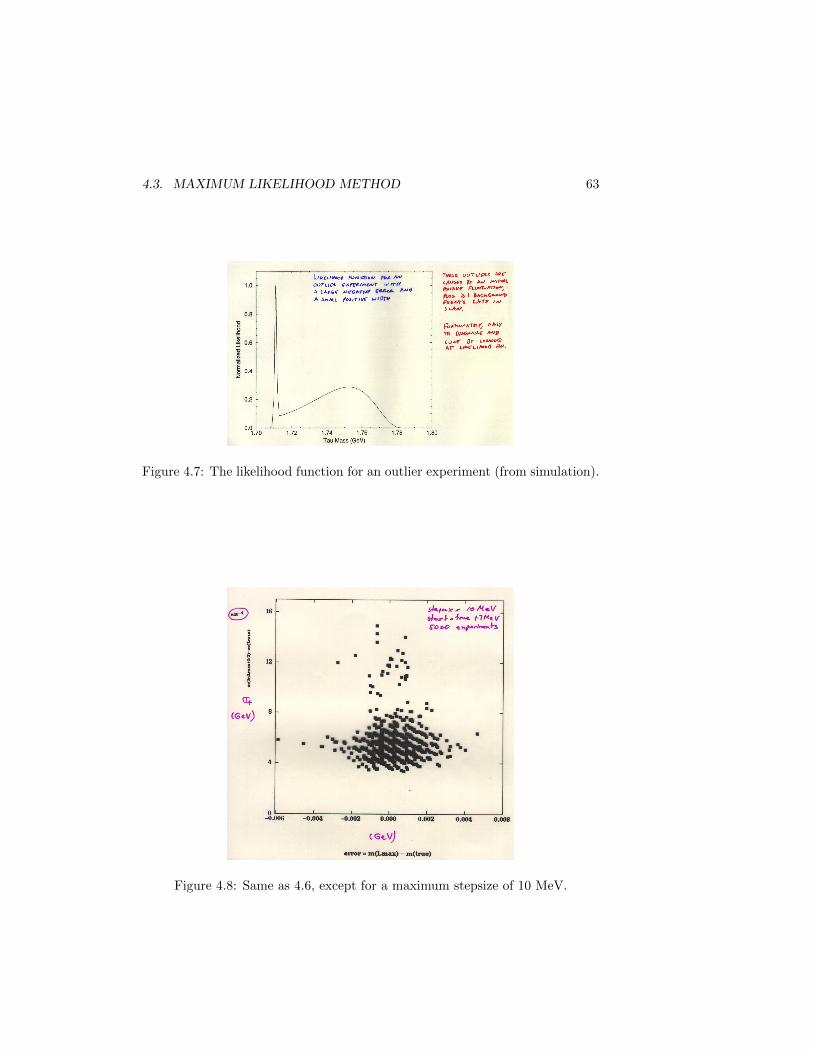
Figure 4.6 shows results from 5000 simulated experiments, in which thefirst energy step was 7 MeV above the true mass (as happened in the actualexperiment). The vertical axis shows an estimate for the size of the positiveerror bar. This estimate is based on the likeliood function and will be discussedin the chapter on interval estimation. Here it will suffice to note that this isan estimate for the size of the fluctuatoins to be expected in the measurement.The horizontal axis shows the error of the measurement, that is, the MLE massminus the true mass. Most of the 5000 simulated experiments are in the tightclump of points around zero on the horizontal axis. However, there are longtails in the plot, and these are worrisome as they indicate the possibility oflarge errors in a measurement that is supposed to be precise at the level oftenths of an MeV. We’ll refer to experiments falling in these tails as outliers. Ofmost concern are those with a large deviation from the true value, but a smallestimated error, since in these cases the error estimate does not reflect the trueerror made.

Figure 4.7 shows the likelihood function for one of the outlier experimentswith a small estimated error. These outliers have this characteristic likelihood


Figure 4.6: Graph of the estimated upper uncertainty on mass vs. the error inthe measured mass, from simulations of the experiment. The maximum stepsizeis here 100 MeV.

function, with a sharp peak at a low mass, and a broad peak at higher mass.The source of these outliers is traceable to an initial positive fluctuation causinga large step to low mass, then a background event occurring late in the scan.Fortunately, this situation is easily recognized by the form of the likelihoodfunction, and did not occur in the actual experiment. In fact, the maximumstepsize allowed in this simulation is 100 MeV, practically no constraint onthe step size. A more realistic maximum step size (the actual maximum issomewhat unclear) is 10 MeV. Figure 4.8 is the same as Fig. 4.6, except for a10 MeV maximum energy step (note that there is a multiplier of 10−4 on thevertical axis. The outlier problem is now essentially gone.

Finally, we can look at the expected bias in the measurement. Figure 4.9shows the bias as a function of the maximum stepsize. Two curves are shown,one for the driving channel alone, and the other for the measurement combiningall channels. For resonable step sizes, the bias is of the order of a tenth of anMeV, which is small compared with the other uncertainties in the measurement.


Figure 4.7: The likelihood function for an outlier experiment (from simulation).

Figure 4.8: Same as 4.6, except for a maximum stepsize of 10 MeV.


Figure 4.9: Measurement bias as a function of maximum step size.

4.4 Substitution (Moment) Method

Suppose we have PDF f(x; θ) for random variable X, depending on unknownparameter θ. Any statistic U(X) computed from X has expectation value:

〈U〉 =

∫u(x)f(x; θ)dx = φU (θ).

If φU is invertible, we have:θ = φ−1U [〈U〉].

Thus, we can define a plausible estimator for θ if we substitute the sampleaverage mu = 1

n

∑ni u(xi) for the expectation value of U :

θ = φ−1u [mu].

This method is often very easy to apply (and is sometimes applied withouteven thinking about it), but there is no reason to expect it to be efficient.

A common application of the moment method is in the estimation of parentangular distributions as in a scattering experiment. For example, suppose wewant to estimate a in an assumed angular distribution of the form:

dσ

dΩ= A(1 + a cosϑ), (4.29)

where our measurement consists of the n IID samplings, x1, . . . , xn of x =cosϑ.

Taking U(X) = X, we have

〈X〉 =

∫x(1 + ax)dx/2 = a/3 = φx(a).

This is readily inverted, and we obtain the estimator for a:

a =3

n

n∑i=1

xi. (4.30)

4.4. SUBSTITUTION (MOMENT) METHOD 65

Case study: CP violation via mixing

For a more involved example, consider the measurement of CP violation viamixing at the Υ(4S). This measurement involves measuring the time differencebetween two B meson decays. The PDF for this time random variable may bewritten:

f(t;A) =1

2e−|t|(1 +A sinxt),

where t ∈ (−∞,∞), x = ∆m/Γ is known, and A is the CP asymmetry param-eter of interest.

In the early days, when the experiment was being designed, there wassome small dispute concerning the importance of the “dilution factor” in whatamounts to a moment method. We have the tools to analyze this now.

The simplified analysis under discussion was to simply count the number oftimes t < 0, n−, and the number of times t > 0, n+. The expectation value ofthe difference between these, for a total sample size n = n− + n+, is:

〈n+ − n−〉 = nxA

1 + x2.

This is readily inverted, leading to the estimator:

A = d−1n+ − n−

n,

where d = x/(1 + x2) is known as the “dilution factor”. We note that A is bydefinition an unbiased estimator for A. The question is, how efficient is it? Inparticular, we are throwing away detailed time information – does that mattervery much, assuming our time resolution isn’t too bad?

First, what is the variance of A? For a given n, we may treat the samplingof n± as a binomial process, giving:

δA = d−1√

(1− d2A2)/n.

Second, how well can we do, at least in principle, if we do our best? Let’suse the RCF bound to estimate this (and argue that, at least asymptotically,we can achieve this bound, e.g., with the maximum likelihood estimator):

For n independent time samplings, the RCF bound on the variance of anyunbiased estimator for A is:

δ2A ≥ 1/〈

[∂

∂A

n∑1

log f(ti;A)

]2〉 (4.31)

≥ 1/n〈(

sinxt

1 +A sinxt

)2

〉. (4.32)

Performing the integral gives:

δ2A =1

n

∞∑k=1

A2(k−1) x2k(2k)!

[1 + (2x)2][1 + (4x)2] · · · [1 + (2kx)2].


Figure 4.10: RCF bound on error in asymmetry parameter estimators.

This function is graphed as a function of the asymmetry, for selected valuesof x, in Fig. 4.10. The value of closest to the true value is 1/

√2. Figure 4.11

provides a comparison of this bound with the variance from the moment method.We may conclude that, especially for large asymmetries, significant gains maybe obtained by using the detailed time information. The actual measured valuefor A is about 0.7.

4.5 Least Squares Method

A third popular method is the method of Least Squares Estimation [A nicediscussion of this subject appears in: F. T. Solmitz, Ann. Rev. Nucl. Sci., vol14, 375-402 (1964)]:

Definition 4.7 Given a set of observations x1, . . . , xn, with expectation val-ues g1(θ) = 〈x1〉, . . . , gn(θ) = 〈xn〉 and covariance (moment) matrix M , then

the set of parameter values θ that minimizes the quantity:

S = (x− g)TM−1(x− g) (4.33)

is called the Least Squares Estimate (LSE) for θ.

The intuition behind this method is that the best “fit” to the data is thatset of parameter values that minimizes a measure of the deviations betweenthe “model” (g(θ)) and the data. In this case, the measure of a deviationis the squared difference, weighted according to the moment matrix, so thatimprecise data with large variances carries less weight than precise data withsmall variances.

4.5. LEAST SQUARES METHOD 67

Figure 4.11: The variance according to the moment method divided by the RCFbound on the variance in the asymmetry parameter estimates.

If the xi are sampled from a multi-variate normal distribution with knownmoment matrix, then the LSE is the same as the MLE. This is clear since S iswhat appears in the exponential of the normal PDF, with a factor of −1/2. Wealso have that S is distributed according to a χ2 distribution with n− r degreesof freedom, where r is the number of independent parameters being estimated.We will later see that this provides us with a test for “Goodness of fit”, althoughthis is already intuitive – smaller values of S mean that the agreement betweenthe data and the model is better than for large values of S.

Even if the observations are not normally distributed, the LSE may be useful,for example, if the distribution is approximately normal.

4.5.1 LSE - Sample Application

Suppose our data consists of a histogram which we wish to fit to some model,including the estimation of some parameters.

In general, the histogram bin contents are described by Poisson distribu-tions, rather than normal distributions. However, if the contents are large, thenormal approximation may suffice. In this case, the bins are independent, sothe moment matrix is diagonal. The moment matrix is not actually known, soit must be estimated in order to apply this method. There are two commonapproaches to estimating these variances to be used in the fit:

1. Use the value of gi as the estimated variance for the ith bin. In this case,the variance estimate changes as the parameters are varied. In principlethis approaches correct estimates as the fit approaches correct parameter


values, but allowing the variances to change as the minimum is searchedfor may result in an unstable fit.

2. Use the value of xi (observed bin contents) as the estimated variance forthe ith bin. This approach is likely to be more stable, but has the dangerthat downward fluctuations in bin contents will carry more weight thanupward fluctuations, introducing a downward bias on the estimated model.

One rule-of-thumb is that the normal approximation is typically reasonable(and the χ2 goodness of fit valid) if each bin has at least 7 counts, althoughhigher values are also used for this minimum. Note that it is quite permissibleto combine bins until this is satisfied. The bin width need not be constant.

4.5.2 Linear Least Squares Methodology

Suppose the expectation values gi for xi are n linear functions of the r param-eters θ:

〈x〉 = g = g0 + Fθ,

where F is a matrix with n rows and r columns. It is convenient to translatethe measurement vector by the constant vector g0:

y = x− g0. (4.34)

Then

S = (y − Fθ)TM−1(y − Fθ). (4.35)

It is readily demonstrated that 〈y〉 = Fθ, and that Var(y) = M .

We obtain θ, the values that minimize S by:

∂S

∂θi

∣∣∣θ

= 0. (4.36)

Or, with

∇θ ≡

∂∂θ1· · ·∂∂θr

, (4.37)

we have (noting that taking the transpose of a scalar does nothing)

0 =[∇θ(y − Fθ)T

]M−1(y − Fθ) +

[(y − Fθ)TM−1∇Tθ (y − Fθ)

]T ∣∣∣θ

= 2[∇θ(y − Fθ)T

]M−1(y − Fθ)

∣∣∣θ

(4.38)

= −2FTM−1(y − F θ). (4.39)

Let H ≡ FTM−1F ; this is an r × r matrix. Then we may write

FTM−1F θ = FTM−1y, (4.40)


or Hθ = FTM−1y. Assuming H is non-singular, we solve for estimator θ:

θ = H−1FTM−1y. (4.41)

Let us check the expectation value of this estimator:

〈θ〉 = 〈H−1FTM−1y〉 (4.42)

= H−1FTM−1〈y〉 (4.43)

= H−1FTM−1Fθ (4.44)

= H−1Hθ (4.45)

= θ. (4.46)

Our estimator is unbiased. We leave it as an exercise to demonstrate that

cov(θ) = H−1, (4.47)

and that we may write:

S = (y − F θ)TM−1(y − F θ) + (θ − θ)TH(θ − θ) (4.48)

Notice the similarity between Eq. 4.48 and Eq. 4.11. Suppose that oursampling distribution is in fact multivariate normal:

f(y; θ) = A exp

[−1

2(y − Fθ)TM−1(y − Fθ)

], (4.49)

where we leave the determination of the normalization A as an exercise. Theconditions giving θ are r linear functions of the observations x. Imagine thatwe “complete” this linear transformation with a transformation that takes then variables y to the r variables θ and n − r variables z, constructed to beindependent of the θ. We thus conclude that the likelihood function must be ofthe form:

L(θ; θ, z) = exp

[−1

2(y − F θ)TM−1(y − F θ)

]exp

[−1

2(θ − θ)TH(θ − θ)

].

(4.50)

This is just the original PDF, with θ replaced by the estimators θ, times a“correction term”, taking into account that θ may differ from θ. We have splitthe likelihood into two independent probabilities, the probability that we willobserve θ, given θ, times the probability that we will observe y given a PDF withparameters θ. The second exponential is the PDF for θ. The first exponentialcompares y with the predictions based on θ. But the θ are r linear functions ofthe y’s, so there are really only n− r variables left. Thus, the first exponentialexpresses the probability distribution in the remaining n − r variables z, andthe quadratic form:

χ2(θ) = (y − F θ)TM−1(y − F θ) (4.51)

is distributed according to the χ2 distribution with n − r degrees of freedom[we’ll demonstrate this connection in class]. We will find this useful in testingwhether the data are consistent with the “model” expressed by 4.49.


4.5.3 Non-linear Least Squares

In general, we are not lucky enough to have a linear problem. In this case:

1. First, see whether it is equivalent to a linear problem.

2. Second, if you don’t need to do it often, plug it into a general-purposeminimizer. This is usually very compute intensive compared with othermethods, so should only be done if you won’t need to do it very manytimes.

3. Or, third, especially if you need to do it many times (e.g., track fitting orkinematic fitting) it may be a good approximation to linearize the problemvia a Taylor series expansion about some starting value for the parameters.The process is iterated until convergence is (hopefully) attained.

The procedure in the third option is as follows: Make a Taylor series expan-sion of the function giving the expectation values about some initial guess forthe parameter values:

gi(θ) = gi(θ0) +

r∑j=1

(θj − θ0j )∂gi∂θj

∣∣∣θ0

+ . . . (4.52)

It is desirable to pick a starting θ0 that is near the value that minimizes S, inorder for the fit to converge well. Neglecting the higher order terms, we have aproblem of the form:

g(θ) = g0 + Fθ, (4.53)

where

g0 = g(θ0)− Fθ0, (4.54)

Fij =∂gi∂θj

∣∣∣θ0. (4.55)

We then solve this linear problem as discussed already. Often the first solutionwill not be close enough to the desired minimum. In this case, we re-expandabout the new estimate and iterate for a new solution. We may continue toiterate until convergence is achieved, as may be determined by small differencesbetween iterations.

4.5.4 Constraints

When we find the minimum of

S = (x− g)TM−1(x− g) (4.56)

we are attempting to find those functions g which give a “best fit”. The g aren functions of r parameters. Thus, there are n − r equations relating the gi’s,that is, we have constrained the possible values of g by using these equations.


We may approach the problem differently: Let us take g themselves as n “inde-pendent” parameters, and use the method of Lagrange multipliers to introducethe constraints on the allowed values for g.

Thus, we may write:

S = (x− g)TM−1(x− g) + 2λT c(g, u), (4.57)

where the factor of two is introduced for convenience, and c are k equations ofconstraint. That is, they are equations of the form c = 0. These constraintequations could, perhaps, depend not only on g, but also on some m additionalunknowns u. The λ is a vector of k Lagrange multipliers. The desired “best fit”is obtained by minimizing S with respect to g, u, and the Lagrange multipliers.

If we are lucky, c is linear in g and u, otherwise we may perform a linearapproximation and iterate. Thus, assume:

c(g, u) = c0 +GT g + UTu, (4.58)

where G is a k × n matrix:

Gij =∂cj∂gi

∣∣∣g0,u0

, (4.59)

and U is a k ×m matrix:

Uij =∂cj∂ui

∣∣∣g0,u0

. (4.60)

Then

S = (x− g)TM−1(x− g) + 2λT c0 + 2λTGT g + 2λTUTu. (4.61)

Setting the derivatives equal to zero with respect to g, u, and λ yields theequations:

0 = −M−1(x− g) +Gλ (4.62)

0 = Uλ (4.63)

0 = c0 +GT g + UT u. (4.64)

To solve these equations, we may first eliminate g and then λ to obtain

u = −K−1UH−1(c0 +GTx), (4.65)

where H is the k × k matrix H ≡ GTMG, and K is the m ×m matrix K ≡UH−1UT . Then we back-substitute to find the estimators for g and λ:

λ = H−1(c0 +GTx+ UT u (4.66)

g = x−MGλ. (4.67)

Letting E ≡MG and J ≡ UH−1, we may express our estimators as:

u = −K−1J(c0 +GTx) (4.68)

λ = H−1(c0 +GTx+ UT u) (4.69)

g = x− Eλ. (4.70)


4.5.5 Explicit case of two dimensions

Consider the case of sampling from a bivariate normal distribution with commonmean and known moment matrix.

χ2 = (x− ϑ)TM−1(x− ϑ), (4.71)

where

x =

(x1x2

), ϑ =

(θθ

), (4.72)

and

M =

(σ21 ρσ1σ2

ρσ1σ2 σ22

). (4.73)

We form the least-squares estimator, θ, for θ according to

∂χ2

∂θ

∣∣∣∣∣θ=θ

= 0. (4.74)

The result is

θ =

x1

σ21

+ x2

σ22− (x1 + x2) ρ

σ1σ2

1σ21

+ 1σ22− 2ρ

σ1σ2

. (4.75)

4.6 Gauss-Markov

We introduce some additional terms at this point:

1. The term error is used to describe the difference between a datum and itsexpectation value, or between an estimator for a parameter and the truevalue of the parameter. We have already used this notion in our statementof the Gauss-Markov theorem.

2. The term residual is used to describe the difference between a datum andthe “fitted” value.

It is readily demonstrated that the LSE is efficient and unbiased if the obser-vations are normal and the parameter functions are linear. However, the LSEhas some favorable properties beyond this, as implied in the following theorem:

Theorem 4.6 Gauss-Markov Consider the linear model for our observa-tions:

yi =

r∑j=1

θjsji + εi, (4.76)

where sji is given, and the “error” εi is sampled from some distribution, notnecessarily normal. If 〈εi〉 = 0 and Var(εi) <∞, then the LSE estimator for θis unbiased and of minimum variances among all linear unbiased estimators.

4.7. BAYES ESTIMATION 73

This property of the LSE is sometimes denoted “BLUE”, for “Best Linear Un-biased Estimator”.

We’ll save the proof of this as an exercise.The “pulls” (or standardized residuals), are a handy way to tell whether the

fit assumptions (e.g., M) are reasonable:

pulli =xi − gi(θ)√

Mii − (FH−1FT )ii.

If all is well, the pulls should be N(0, 1) distributed for normal sampling. (Ex-ercise)

Note that there is another term in common use, which is easily confused.The “normalized residuals” are given by:

xi − gi(θ)√Mii

.

4.7 Bayes Estimation

The Bayesian approach to parameter estimation is very similar in method tomaximum likelihood estimation, with one important difference: In Bayesianestimation, the likelihood function is multiplied by a prior distribution to obtainthe “posterior distribution”. The maximum of this posterior distribution is thentaken to be the estimate of the parameter. Often in practice, the posterior istaken as a constant, in which case the Bayesian estimator is the same as theMLE.

4.8 Exercises

1. Prove the theorem that an efficient (perhaps biased) estimator for θ existsiff:

∂ lnL(x; θ)

∂θ= [f(x)− h(θ)]g(θ)

. An unbiased efficient estimator exists iff we further have:

h(θ) = θ.

Hint: The RCF bound made use of the linear correlation coefficient, inwhich equality holds iff there is a linear relation:

∂θ lnL(x; θ) = a(θ)θ + b(θ).

2. Show that θ = D(x) is an efficient estimator for θ, if x is sampled fromthe exponential family:

L(x; θ) = exp[A(θ)D(x) +B(θ) + C(x)].


3. If x is a sample from a normal distribution of known variance, show thatx is an unbiased efficient estimator for the mean.

4. What is the bias of the estimator for a in 4.30? Compare its efficiencywith the minimum bound.

5. Generalize the moment method example to an estimator for the strengthof an arbitrary Y`m moment.

6. Is the moment method always consistent?

7. Consider the simple angular distribution problem we have discussed interms of the moment method already, with pdf:

dσ

dΩ= A(1 + a cosϑ),

where our measurement consists of the n samplings, x1, . . . , xn of x =cosϑ.

Find the LSE for a, and compare its properties with the estimator fromthe other methods.

8. Consider the simple angular distribution problem we have discussed interms of the moment method already, with pdf:

dσ

dΩ= A(1 + a cosϑ),

where our measurement consists of the n samplings, x1, . . . , xn of x =cosϑ.

Find the MLE for a, and compare its properties with the estimator fromthe moment method.

46 - california institute of technology

Documents