(47) on the analysis of multidimensional contingency table...

(47)

ON THE ANALYSIS OF MULTIDIMENSIONAL CONTINGENCY TABLE DATA USING LOG LINEAR MODELS

Geoffrey A. Clark

Introduction

Department of Anthropology, Arizona State University, Tetipe, Arizona öSüöl, U.S.A.

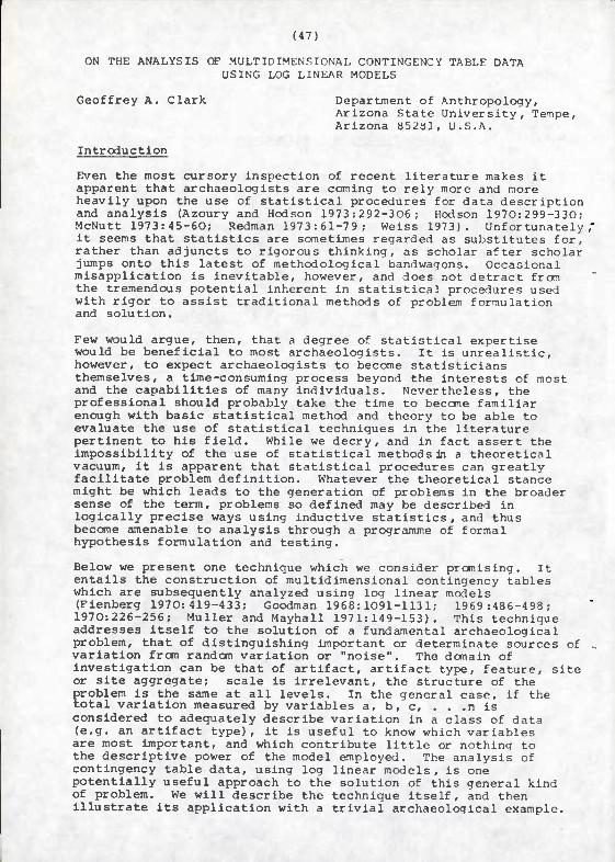
Even the most cursory inspection of recent literature makes it apparent that archaeologists are coming to rely more and more heavily upon the use of statistical procedures for data description and analysis (Azoury and Hodson 1973:292-306; Hodson 1970:299-330; McNutt 1973:45-60; Redman 1973:61-79; Weiss 1973). Unfortunately,' it seems that statistics are sometimes regarded as substitutes for, rather than adjuncts to rigorous thinking, as scholar after scholar jumps onto this latest of methodological bandwagons. Occasional misapplication is inevitable, however, and does not detract fron the tremendous potential inherent in statistical procedures used with rigor to assist traditional methods of problem formulation and solution.

Few would argue, then, that a degree of statistical expertise would be beneficial to most archaeologists. It is unrealistic, however, to expect archaeologists to become statisticians themselves, a time-consuming process beyond the interests of most and the capabilities of many individuals. Nevertheless, the professional should probably take the time to beccme familiar enough with basic statistical method and theory to be able to evaluate the use of statistical techniques in the literature pertinent to his field. While we decry, and in fact assert the impossibility of the use of statistical methods In a theoretical vacuum, it is apparent that statistical procedures can greatly facilitate problem definition. Whatever the theoretical stance might be which leads to the generation of problems in the broader sense of the term, problems so defined may be described in logically precise ways using inductive statistics , and thus become amenable to analysis through a programme of formal hypothesis formulation and testing.

Below we present one technique which we consider promising. It entails the construction of multidimensional contingency tables which are subsequently analyzed using log linear models (Fienberg 1970:419-433; Goodman 1968:1091-1131; 1969:486-493; 1970:226-256; Muller and Mayhall 1971:149-153). This technique addresses itself to the solution of a fundamental archaeological problem, that of distinguishing important or determinate sources of variation fron random variation or "noise". The domain of investigation can be that of artifact, artifact type, feature, site or site aggregate; scale is irrelevant, the structure of the problem is the same at all levels. In the general case, if the total variation measured by variables a, b, c, . . .n is considered to adequately describe variation in a class of data (e.g. an artifact type), it is useful to know which variables are most important, and which contribute little or nothing to the descriptive power of the model employed. The analysis of contingency table data, using log linear models, is one potentially useful approach to the solution of this general kind of problem. We will describe the technique itself, and then illustrate its application with a trivial archaeological example.

(48)

Multidimensional Contingency Table Analysis

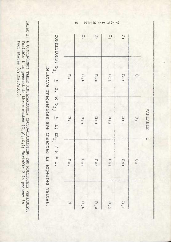
A contingency table may be defined as a matrix or an array of counts or observations which simultaneously cross-classify objects as belonging to one or more variables , which themselves are present in two or more mutually exclusive states.

A simple two-way contingency table is presented in Table 1. Note that objects are classified according to two multistate variables: Variable 1 is present in three states (C.,C ,C ); Variable 2 Is present in four states (C ,C ,C ,C ). A ^ ccrimon approach to this kind of classification p?oblem is to Insert raw counts in all cells and convert these data to relative frequencies. This, of course, is done by using the marginal totals as estimators; that is, one can convert to percentages using row totals, column totals or N (the table total) as estimators.

By converting to percentages, one obtains an empirical estimate of the probabilities of obtaining an observation with a given value on Vciriable 1 and a given value on Variable 2. Counts are thus converted to expressions of probability:

(1) n,. / N = p..

The constraints are those which apply to all probability statements: no given probability can be less than zero (i.e. negative), nor can any given probability exceed one. All probabilities must sum to one.

(2) Pij>0 p^. ^

(3) P^.4 1 '• ^Pij =_^VL ij N

The contingency table format is usually applied to non-metric data; however, it can be used with metrical data (i.e. data which have a continuous underlying distribution) by establishina class intervals and Inserting counts in them.

Conventionally, data of this sort are analyzed by using a Chl- Squared Test (Slegal 1956:42-47, 104-111, 175-179). One might ask whether the horizontal distribution is the same for one state within a variable as it is for another, or, generally, how do the relative cell frequencies vary from cell to cell? Are the distributions homogenous or not? Those familiar with X , however, will recognise that two constraints limit its usefulness. The first is that expected cell counts must be greater than or equal to some number (usually 5 , sometimes 3) ;

(4) e^.. >, 5; e. j > 3

Failure to meet this constraint usually leads to the collapsing of the table, which in turn results in lost information. Second, one cannot analyze above 2-way Interactions using X .

(49)

Contingency table analysis allows for expected cell counts to be zero, and permits the examination of higher order (i.e. greater than 2-way) interactions. It also allows for zero raw cell counts, whereas an unmodified X does not. The method2is not, however, completely free of constraints. As with X , a multinomial distribution is assumed for the data tabulated as a prerequisite for obtaining cell estimates. One consequence of a multinomial distribution is that cells are theoretically independent; thus marginal totals can be used as estimators. A second constraint is that, for obvious reasons, no marginal total used in calculations can contain a zero.

2 In contingency table analysis , as in X , one generates expected counts using the marginal totals derived from a model designed by the investigator. The expected values are the compared with the observed values. The principle difficulty lies in casting investigator-generated hypotheses into explicit statements of relationship between variables. If these hypotheses are properly defined, they can be expressed in the form of a linear equation. It is in the sense of an equation that we use the term "model" here. It is more convenient to express the model in terms of the natural logarithms of the cell probabilities than it is to try to deal with the cell probabilities themselves. For this reason, the model is said to be a "log linear" one.

Those readers familiar with statistical applications will note the similarity between the model described above and the analysis of variance (ANOVA) model. It is useful to consider the case of the ANOVA model in order to explicate and define the terms in the CTAB equation.

Consider the case of a 2-way ANOVA with no replications (the number of replications simply refers to the number of observations taken in each cell). The equation is of the form:

(5) Y^.^ =/'+ <<i * /?j + /i^ + E ijn

where y^j_ specifies the row, column and individual within the cell,^ Is a constant (the grand mean of the expected cell counts), ^ . is the row effect,^ . is the column effect,Y.. is the row/column interaction ternl, and E.. is the error tirm. If n = 1 (i.e. if only one observation is iSken per cell), then it is not possible to estimate the interation between the two variables and the formula collapses to:

(6) Vij =7^ + '^i + /^j + Eij

'der to cast the Two-Way ANOVA equa y replace the above terms with the

(7) log p^. = [l] + [A]^ + [B],

îcii 5 si

logs of the expected counts, [Aj is the main effect due to A.

In order to cast the Two-Way ANOVA equation into CTAB form, we simply replace the above terms with the relative cell frequencies:

where log p.. specifies the natural logarithm of an observation identified By its subscript, where £l] is the grand mean of the

0) M-H C O. O

</) <D Vt

LU Ö - m m m -H

^ a ai

C) Ä 0)

X 1- .H +J

gâ-

OJ EH

g O M

IV) Mt-'Cd>MS)><î

o w

iv>

O O 3 O H H M O 3 W ••

w •o fD H- M C-l.

P3 et- H- 1 V < fD

O i-b V*

4 fD 3 ^ O C fD •ö t3 H- O C_i.

h^ fD M |v

(U 4 M (D \*i

H- M ri 13 w H- fD C-l.

4 et \ fD & 3

P II M

M fD • X •Ö fD Cl et fD P-



O CU

3 • 13 • <41

3 • 3 •

> H > CO

M

(50)

and fß]. is the main effect due to B.. The main effects refer ta a specified set of marginal"'totals selected by the model to be fit. The method will generate expected cell values, on the basis of this particular subset of marginal totals. These expected values are referred to as maximum likelihood estimates; they express the most probable values for the observed cell counts to take on IF THE MODEL CHOSEN IS CORRECT.

The technique then compares the maximum likelihood estimates with the original observed cell counts. If the main effects fit by themselves, then it can be assumed that the interaction terms are negligible (i.e. they approximate zero). If the expected values generated by the model do not agree with the observed values, then a non-zero interaction exists. The marginals used to generate the expected values are the highest order interactions in the model. The Importance of zero marginals becomes clear: if any marginal total sums to zero, then no estimates can be obtained frcxn it. Zero marginals are usually eliminated by adding a small constant (e.g. .01) to all tabulated values.

Given the similarity of this method to analysis of variance, it is pertinent to ask what advantages CTAB might have over ANOVA. The main reason contingency table analysis is to be preferred is that it is not characterized by the strong underlying assumption of normality which is a feature of analysis of variance. Also, zero cell counts are possible in CTAB analysis; they must be corrected for in ANOVA.

Model Formulation

We turn now to the question of model formulation. It is obvious that given even a few primary variables, a comparatively large number of models can be generated; 2 models will result for n primary variables. Two major approaches have been developed to generate and evaluate models of the form described above. They can be labelled the Fienberg and the Goodman approaches, although those authors are not unique in their contributions to the problem.

The Fienberg Approach

Stephen Fienberg (1970:419-433), a statistician at the University of Chicago, has developed a method which takes a series of models, each one of which represents a set of explicit hypotheses about the data, orders these models into a hierarchy and evaluates that hierarchy on the criteria of adequacy and parsimony. Hierarchical models are models (in this case equations) ordered from simple to complex, such that any given model contains all of the terms in the model which precedes it. In the context of a contingency table analysis, this means that if an interaction term (AB) occurs in the model, then the primary variables (A) and (B) must also be included. It might be the case that the investigator regards the primary variables (A) and (B) by themselves as meaningless; nevertheless, they

(51)

must be included in the erruation.

The Fienberg approach has the arlvantaqe of qreater precision, but assumes considerable forehand knowledae of the behaviour of the data. Considerable thought about the hypotheses to be tested is a prerequisite, but the technioue is more "elegant" in the mathematical usage of the word. It has the disadvantage that it might not always prove to be adequate if the behaviour of the data is completely unknown, or if its behaviour is "masked" by unforeseen and complex interactions.

The Goodman Approach

The second approach, outlined in a series of papers by Leo Goodman (1968:1091-1131; 1969:486-4 98; 1970:226-256), fits the most complex (most complete possible) model to the data, and then tests whether the effects due to each term are zero or not. In this way the terms in the model are successively reduced until all zero terms are eliminated, resulting in the simplest, adequate model.

The Goodman approach has the advantage that it cannot fail to produce a model which adequately describes the pattern of variation in the data. The variables isolated, however, might be so complex that they defy interpretation. No previous knowledge of the data is required under the Goodman approach; there is no necessity to formulate explicit hypotheses. By comparison with Fienberg's approach, this method is "sloppy" in the sense that a lot of extraneous information goes into the construction of the "most complete" model. In either case, the final objective is to isolate the simplest and most comprehensive model.

Decision Making Criteria

Given that a number of models will be generated by the analysis, one must face the problem of how these models are to be compared if the isolation of a single "best" model is the objective.

The obvious first step is to determine whether a model "fits" the data or not; that is, whether the expected cell counts are good predictors of the observed cell counts. It will probably be the case that a number of models "fit" the data in the sense defined above; the second step is to make a choice among them. The only constraint for comparison is that the models be of a hierarchical nature (i.e. ordered from simple to complex); if they are not, the tests used to compare them cannot assume independence.

2 The two models most frequently used to compare models are X and the log likelihood ratio (log^). Chi-squared tests are widely known and used; they require no further comment. The lc3g likelihood ratio also makes use of the X distribution. If X = the likelihood ratio, the expression

(8) - 2 log A approximates the X distribution.

The log likelihood ratio is obtained by taking the log of each quotient (observed / expected) cellwise, summing the logs, and multiplying by two:

(52)

(9) - 2 log A = 2 2_ ( loq O/E).

The values for the X distribution are well tabulatod. 2

Although both X and log ?» are suitable methods for testing the difference between models, log ^ has the advantage that it can be partitioned into independent parts such thit each partition is an independent test of a particular model. Chi-squared cannot be so partitioned. Log ^ is also more stable for small values (4. 5) than is X .

The steps discussed so far are simple but tedious i" done by hand. There is, however, a computer progra-n (CTAB) in the SNAP series (University of Chicago) which provides output specifying cell estimates, log li)<elihood ratio and degrees of freedom fit for each model tested. All that it is necessary to do,is to draw up a table showina the loa lil'.elihood ratios and degrees of freedom fit for each model. Since the models are hierarchical, one can use these statistics to tost differences between them. Evaluation proceeds pairwisp frm the most complex model to the simplest. Two stopnina criteria are employed: (1) when Model X adeouately descril^es the data and Model Y does not, choose Model X; (2) when Model X and Model Y both describe the data, and there is a statistically significant difference between them choose Model X. Because of the hierarchy and the evaluation procedure used. Model X will always be the simpler of the two.

An Archaeological Example

An illustration of the method using a concrete archaeological example is presented below. Data come from an assemblage Vcnown as the Asturian of Cantabria (Vega del Sella 1923; Clark 1971a; 1971b), found in the provinces of Asturias and Santander, on the north coast of Spain. Sites consist of semi-brecciated midden deposits located in cave mouths along the Cantabrian littoral. Large, crude quartzite tools form an important component of the lithic industry. The assemblaae dates to the early Holocene (8,900-6,000 BP)(Claris 1971b:1245-12b7).

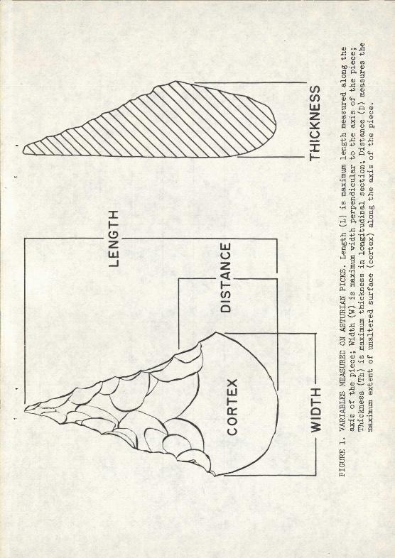
The sample selected for analysis consisted of 92 pointed, uni-facial quartzite core tools called "Asturian Pic^;s". These Implements are the so-called "guide fossil" for the industry. Each pick was classified by site and by a series of four rather trivial dimensions: length (L), width (W), thickness (Th) and distance (D)(Fig. 1). Dimensions were trivial because little confidence can be placed in provenience data, owing to inadequate cataloging procedures. The high probability of mixed collections did not justify more elaborate recording of attribute data. Nevertheless, the data selected are adequate to illustrate the method outlined above; however, no attempt will be made to draw culturally relevant conclusions from the analysis.

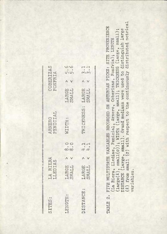
The five variables used are listed in Table 2; the variable "site" was present in six states and each of the four dimensions was subdivided into "large" il) and "small" (r). Subdivisions

(53)

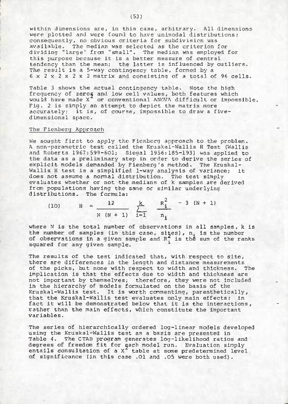
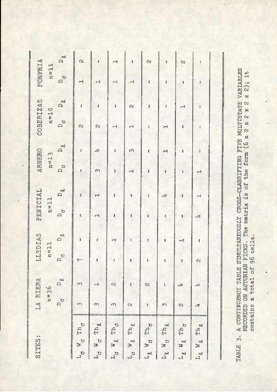
within dimensions are, in this case, arbitrary. All dimensions were plotted and were found to have unLTiodal distributions; consequently, no obvious criteria for subdivision was available. The median was selected as the criterion for dividing "large" from "small". The median was employed for this purpose because it is a better measure of central tendency than the mean; the latter is influenced by outliers. The result is a 5-way contingency table, formed by a 6x2x2x2x2 matrix and consisting of a total of 96 cells.

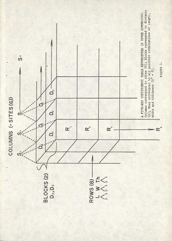
Table 3 shows the actual contingency table. Note the high frequency of zeros and low cell values, both features which would have made X or conventional ANOVA difficult or impossible. Fig. 2 is simply an attempt to depict the matrix more accurately; it is, of course, impossible to draw a five- dimensional space.

The Fienberq Approach

We sought first to apply the Fienberg approach to the problem. A non-parametric test called the Kruskal-Wallis H Test (Wallis and Roberts 1967:599-601; Siegal 1956:185-193) was applied to the data as a preliminary step in order to derive the series of explicit models demanded by Fienberg's method. The Kruskal- Wallis H test is a simplified 1-way analysis of variance; it does not assume a normal distribution. The test simply evaluates whether or not the medians of k samples are derived from populations having the same or similar underlying distributions. The formula:

(10) H = ^^ ^ _RJ_ - 3 (N + 1)

N (N + 1) i=l n^

where N is the total number of observations in all samples, k is the number of samples (in this case, sites), n. is the number of observations in a given sample and P. is the sum of the ranks squared for any given sample. ^

The results of the test indicated that, with respect to site, there are differences in the length and distance measurements of the picks, but none with respect to width and thickness. The implication is that the effects due to width and thickness are not important by themselves; therefore, they were not included in the hierarchy of models formulated on the basis of the Kruskal-Wallis test. It is worth ccnmenting, parenthetically, that the Kruskal-Wallis test evaluates only main effects; in fact it will be demonstrated below that it is the interactions, rather than the main effects, which constitute the important variables.

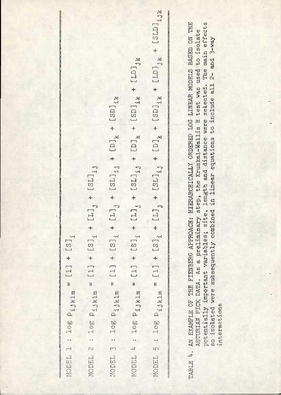
The series of hierarchically ordered log-linear models developed using the Kruskal-Wallis test as a basis are presented in Table 4. The CTAB progrcim generates log-likelihood ratios and degrees of freedom fit for each model run. Evaluation simply entails consultation of a X table at some predetermined level of significance (in this case .01 and .05 were both used).

CO UDMD rH iH < . • • ISI < Lmn 0OCY-) H H (T; K W PH A V A V P3 s o o o fe W J W 1-3

C3 HJ CO HJ « < (E; < <C S < S 1-1 CO »-5 CO

CO K:I CO <: w

o M • • s « o m 1^ W H EH o s s Q H cc; w M K < PM :3 EH

o O H H

oo co ^T ^3-

< A V A V te CO W < M M W tJ W J K Q C5 i-q o >-:i

W K < K < < J <C S < S J i-q i-q CO h^ CO

co w EH H CO

EH

S W

O

< &H CO

H nJ

W Ü O •»< lU -H a ^- bÛ ^^ W H fn -P M rH oj 0) S W Cd H e w &H a > CJ tn Ä T) OS W (U (« W «^-H -P fX, h^ 0) 3 S

bû bD ^ W ••« ;H C -H EH '-^ cd -H !-i M cd H +J -p CQ -H —- W M

U 'H TH • • <H CQ "0 T:)

CQ Ö CQ W O W O >3 O ÜH S -p H M W W Pk •> U Ti 3

10 M <D O fe td W m p! 5 N tH pi Ö M -H -H K ^ ..» 0) 4J S (U-— ^^ Ö ÈH ^ H 0) O en O H > Ü <î O Cd

â u^ dl s " CO Ö Ä o o cd 4^

^1 "-H Q 0) <D T) o W Ö tjÛ (U 4^

K 

<^ to D CO --^ > cd--' Ö

•H H '--' W 'Ö H (U EH cd cd CQ '— ^1 M H:] H M o« cd (k^ ^-w- Q^- t»

OJ

H ^q

< O M H CC H Un II S e n Ü a fe

CO o* •a; Q CNI o M H K II W C n m O o o

oj o O K m w H 2 II K S D •a; O

CO w M CO

CM

^q o? < O M r-t O iH M II S c D W Q Pi<

00 =.« < O M H Ü H W II .J S r> •-1 a

< o< K o U4 VD M 00 œ II

d n < o u

Xi E-i

eu

J3 EH EH EH

Xi EH

a « CM i« W CVJ

S" to OJ M

D CM

X >\o

a o H «H

h «J M Ä CQ +3

S <»H iJ o Ü

I to 03 -H 03 O « œ -ri O U

+J >H OJ j a

O ß

iJ s <U

M pL, VO m c^

'M o

en co <;

o ü H w C

a §

CD

<n UJ

CO It

(0

o o <f)t'

CO q >

O 4J -p

m -H c a TJ * -P OJ

B +J -0 M cm o -0 o w B C p. 01 M o w q B w ^t o o OJ M -H CJ ^. o J3

^^ o -p !« o Cr, rH'-^ T)

O CM 'H << O^ U

Q CO

CO

I I

+

CO

•H •H

a

a

Q CO

Q I—I

+

CO

1—1

+

a H

Q

CO

Q

Q CO

+

CO

I I

+

CO 1 1

CO 1—1

CO 1 p

CO 1—t

CO 1—1

+ + + + + 1—1

1—1

1—1

1—1

1—1

H 1—1

(—t i-i 1—1

m

1 t

a H X "-3 •H

fciO hO bO b3 W o O O O O

r-i M r-t H fH

J i-q HJ ^ ^J W U w w w (J Q Q Q Ü O O O O o s S S S s:

m ta

4J o a a) <*H >. O i-l <M efl

O -P a o (u w -p 4) "0 !Si 01 •( 3 M 0) 0) H t-3 +J n o

Ö C5 K -P

w H H 03 -0 CJ« J 13 D » Ä Ä O O +> -p -H

< » ß K P< (U ß S 4) H -K M -P «03 •• "d

,

h 0) -P Ü ft-H ß

S cfl aJ 3 m ï> a< ^03 V w <; -p 03

E .§•§ «J! -p 03

w EH »H M < o (U H P ft ^(

a o o 03

H ^j'd Ö w a, rH <U O 1-5 H -p •H Oj ;^ ai aJ +J S «3, 'H rH C < M -p O ai X K ß 03 M t3 4) -H

U (U

H +J +J B ra O O ß a < P< 03 •H

1-5

ta CO 0 ß C TJ 0) 'd 'H

H ci -H 0) ß +3 0 Q o a (0 ^^ 0) 0) s ß w • m w CO CO CO CO CO CO CO M 3 aJ 0 0 ß tt II B a a a ùi T) -H 0) -H OJ

<c a <; t>> ta 0) "0 -pu • SoHf>ß-»ff!>ai

cö Cl fn -H m -H +j 4J Of ai^Tao) OJ^HiiaJ co Oo*otoco:3cb,Q'd

1 LTX M 0) Ö ^ a H > CO TS 0 a) ta 0) M O

w 03 CO CO CO CO CO CO CO M aJ ß . t> i« 0) Ä 0 (U ß (d 0 Ü +J

U II a s s s W Ot>>(UoJa)ßaitn

P<,Û (U 0) (l)+JtH-H

0 (U 11 0 ft TJ ta ,„—^ 0 ta CJ 0 -p (U

fc M O fo

Ma)ßß-H'Ö(L>-»<'Ö

<; uu 3 +3 4) s pä ^ 0) OJ 4J -p H

Sw^ otHtHOtiiDßa) w Q<H<iHt|-( ß (D X> <U-P

w o VD vo C\J VO 00 H 0\ u^ -d- 0 -H •r^ +J -H ta 0) O'titi'oiacjfHiu^à W 4) (1) U't^^r-^-H(ü

1 1 (U -iH -H • O •H ^ tn ta ß ß -p O • • <H -H d) (1) +5 0 ß

-^(UrH-PrH^HO 3 tJ 1 td (U 0) <ii t>i 0

M O w hOOtStHli-IrH-H hJ M iH ^ l/^ VD C7\ ir\ -a- ir\ CJ\ iJHO-HO"« ß<i-l

H L/N lA 00 V£) H ir\ t— t— m (UH-ti s-H ß o-H <j^ T* ß -cl 'H ß

-* O ro J- 00 CM VD H -=t EH 0 "Ö -H 0) •• W) g 0) +3 m ta -H

Pt, +JtO'''ß(u+Jta i-:i CO iH t— VO VD VD 1 0 Ä pi ta cd 0 H

CJ u ,a • ß ^ WX oßOi-dH W EH 0 0) 0 13 m

H H W W M -3

EH

o o M 0 M 0 H 0 M 0 s s 0 2 0 S Q S 0 S

S 3 o O O o M M t-i t-i

M

tr" O o t^

ro ftl M • > W H 1-3 M \o H tri

O H W O O O

•^

w a M m M a o w

ON o M 2 W

M ^-^ •flO M >x| »^

P B Il O CO • œ

o H \j\

M O a

ß >

CO ."g o o H

s

M

M

<+ 1^

0 (î

ro o 1 o < 3 P> V

«<! H CD

M- c+ a f!> c+ 0» 0

n- H H- o H- [0

3 3

I H. *! 0 is n '< o

3 O

n (B 4 et p H- O 3 et«

S O O M

O m n

H- C-J.

w H B

II

(—1 J 1 r—1 1—1

O 1—1 1—1

M t-" a t-i E: ö 1 1

Ö •^ 1-3 1 1 1 1

•^ 1—1 ! 1 !V H* + 1—J Ç-i. H- H W-

h"' tv C_ta r—1 C_i. B B + + M P!- 1 1

B + + 1—1

O 1—1 H-

+ 1—1 (—1 •^ s: -1- f M 1—1 1—1

1 1 s: O pr H- (—1

M H3 « B (-• t- f 1 1 1 1 1 1

s: Cl. H- + + C^

•^ H !^ 1—1 B M 1—1 1—1 -1-

H- s: M tj. + + •^ H3 1—1

H 1—1 1—1 a B 1—I 1—1 H H- 1—1

o M B B pr + s: O

1-3 1-3 + + + 1—1 t 1 1 1

GQ W* H' (—1 1—1 1—1

o M fS* CO f s: E: B B t^ o 1—1

H3 o 1—1 H 1—( + -t- 1—1 C_i-

H' H- pf + W 1—1 1—1 C-i.

H W 00 W + 1 1

B t-i s: 1^

O 1^ + 1—t 1 t

+ s: i—( f B 1—j H- 1 1 s:

1—1 H- M w 1—1 + tr' C_t. B f CA

O X s: H r—1

H + 1—1 M t-9 H- -t- f

1 1 + 1—1 C_» 1—I c^ f H 1—1 H-

?!• o t-l Cl.

H « -(- ^3 B 1 1 1—1 +

co

a t-q hJ J EH H :ï :s. > Q Q tH 1^

CO ' w EH < S M EH 00 l-q h^ :s W Q :ï 1^ EH

^ CO CQ :ï Q

fo O

2 ,o M EH O hj h^ w :s • • E^ > a. Q 1^ ^ EH Bi O EH CO CQ P « CO S CQ CQ s < M EH

œ X o (G CU

Q H W EH >H <C J S PQ & iJ M i-:i H :ï :S H « EH S H o CO EH CO CO CO M CO J O W P-,

CO CO CO W CO w W J w u ij m œ K B m < H œ w «a; < M Ü H U EH M K a o M CO œ EH < W M W M < J P > 1^ tS: EH Q > CO CO

FH i-:i a :* H 1-1 W H H S EH M CO l^ [xJ U

CO W ^-l m < H W ce EH < M > CO

•S s (U +5

O) m U m 0) (U Ü H

o 4J

« C\J .a .

•p o d

o -p -p o

o 2 3 0) o< 0)

h •• O cq

CO 0] to Ä O) p H

^H

Ä ß -P O

•H ^H -P 

ai

I

EH CQ W

I

(X. o

o M

(U u CO (U

H

w

^ a P4 o o fn

'M CO EH -d iJ 0) ^ -S CO cd

• n •P +5

S S -p

+J ;H >H O (> ft

S •S !>,

>>H H (U .û +> •H •H

CO ä EO •H O <iH p< 0) -rt to CIJ -0

0) Tl ^ i) Q) T) T) U •H 01 to M C (Ü O Vi Ü

g

H (-:)

I

U u (U > o o

+ I—I

I I

+ r—I IS

+ I—I

I I

+ I—I

i—I

+ I—I

Q I I

+

E-i CO

+ I—I

I I

+ I—1

+

EH Q

+

EH Q

+

CQ U Q W

EH I I

+

+ I—I

+

IS EH CO

(—1 f—1 1—1

J J j r—1 ^ B EH ^ ^ Q Q IS CO CO CO ü 1 1 1 t I 1

CO 1—1 + + +

EH I 1

+ t—1 1—1 (—I

^ J ^ IS IS IS « Q Q CO CO CO 1—1 1—1 1 1

+ r—I

1 I

+ r—I is

+

Q

+ r—1

CO Ll_l

1—1

CO 1 1

1—1

CO 1 i

1—1

CO 1 F

1—1

CO 1—1

1—1

CO 1 1

1 1

m 1—1

+ + + + + + + ( 1

1 1

t—I

1—1

1—1

1—1

1—1

rH 1—1

1—1

rH 1—1

1—1

rH 1—I rH

1 1

e 0 a a a a i iH rH H H H •-\ r- AÎ X M M M M ^ •'-D •rj •TJ •rj "-3 •ra 'T

•H •H •H •H •ri •H T

a a a a a a a M bO w 60 bû bû bO O o o o o o o i-l r-{ <-{ •-{ rH rH H

C3

hJ ij hJ hJ hJ J J w w w td w w w Q o Q Q Q Q (U O o O O O O C) S s S S S S s

1 •H

VI a -d s». 01 •p T) •H

ä 0) tlû H CJ o ^

fH Ul o

g <M

(U 'Ö +J ai

-p (U cd m Ö fi •H X a •p •H

H >. (U H a 4) o h

oj 0) +j en et) +J U ft () •H PI ^ ;H CJ O m () ," a ?l

•H crj

(d . rH w i) T) •p O 01 a a

•H C) +J Ä m -p (U

-p t) ai Ä (U •P Ä

+J Ht

•p Vi o « fe c • o «1 •H

1-J -p w CJ H 0) O ft >; [Q

Ö ^ •H

w (U H Ä

-P « W !>. t) ," D W •P

ss -P

s U O

IrH ft

0\

w 1-1

(54)

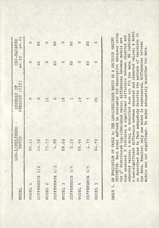
Models which are SIGNIFICANTLY DIFFERENT (S) for specifiedod are those which DO NOT fit the data; these are eliminated. Models which are NOT SIGNIFICANTLY DIFFERENT (NS) adequately describe the pattern of variation in the data; these are retained and further evaluated. Differences between models retained are also tested by the log-likelihood ratio.

Table 5 presents the evaluation of the models formulated on the basis of the Kruskal-Wallis H test. The result is clearcut; no model adequately describes the observed data. It is possible, then, to eliminate Models 1-5 from further consideration; terms expressing main effects are not adequate in themselves to explain or describe variation in the data.

The Goodman Approach

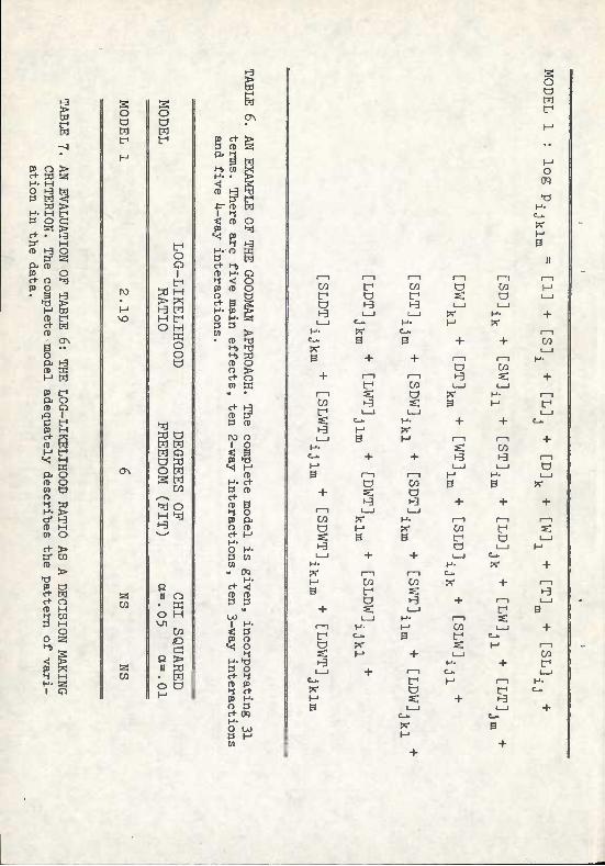
Given the failure of one set of explicit hypotheses, the investigator has the option of defining other sets, on the basis of different criteria, or resorting to the Goodman approach to isolate important variables. As noted, the Goodman approach defines a single model incorporating all main effects and all possible interaction terms (Table 6). In this case, the model contains a total of 31 terms, including the main effects, 10 2-way interactions, 10 3-way interactions and 5 4-way Interactions. As expected, the model fits the data in that it adequately describes them (Table 7); however, no distinction can be made between those variables which are important and those vrfiich are not. The results are, at this stage, uninterpretable. As in analysis of variance, however, relative estimates of the effects in the model can be obtained.

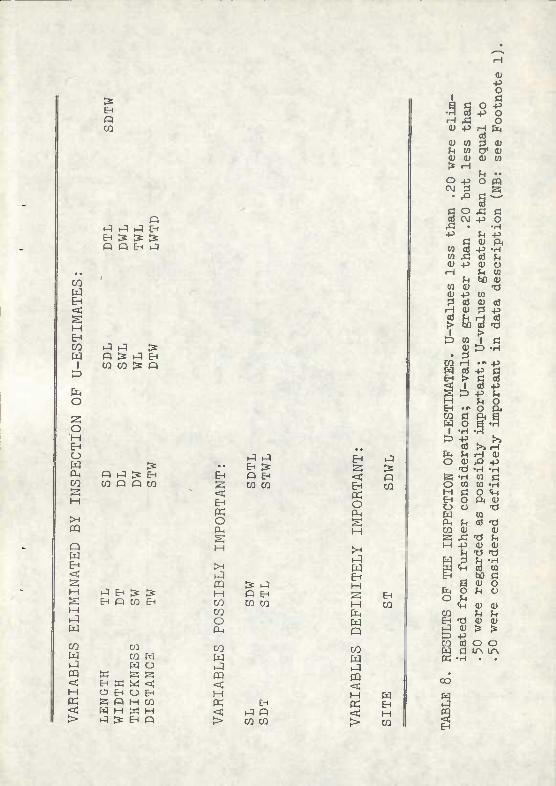
For each model tested, the CTAB output produces statistics called estimated U-values. These assess the influence of each term in the equation against the total descriptive power of the equation. VcLriabJ.es with low U-values (4-.20) probably do not play an Important role in data description and may be eliminated. Models can be made ever more explicit by successive runs, systematically eliminating terms with low U-values.

An examination of U-values in the most complete model permitted the elimination of 21 terms (Table 8). U-values less than .20 were regarded as insignificant; associated terms were consequently deleted. * The result is immense simplification; only three terms are regarded as definitely important variables (U-values >.50); six terms are possibly important (U-values >.20 but < .50).

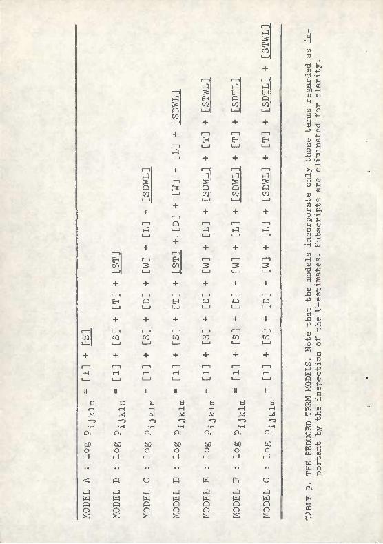
The final step is to construct a set of models using only those terms regarded as important variables. These models are

* It should be noted that this elimination procedure is a practical and useful, but essentially impressionistic approach to the deletion of unimportant terms. Goodman (1969:486-498) advocates a more rigorous evaluation procedure; each term is tested to determine wether a non- zero Interaction exists. Only zero interactions are eliminated.

(55)

presented in Table 9. Inspection of the models reveals three important points. Note first that no 2- and 3-way interaction terms appear to be included. These terns are actually included in any model which contains a 4-way interaction term; because of the program format used, it is not necessary to specify them. Second, note that all of the terms regarded as important are underlined. Other terms are incorporated into the models because of a constraint of contingency table analysis mentioned earlier: all interactions must have their terms defined (i.e. if (AB) is in the equation, (A) and (B) must also be specified). Finally, note that the models are not entirely hierarchical. Inspection reveals that Model A is a subset of B and C; B and C are subsets of D (but not of each other); D is a subset of E and F; and E and F are subsets of G (but not of each other).

The models are ordered from simple to complex, and the partial hierarchy is represented graphically in Fiq. 3. Employing the two stopping criteria defined above, evaluation proceeds from the most ccmplex model (G) to the simplest model (^). Models D, E, F and G all adequately describe the data, moreover, there are no statistically significant differences between them. Model C also describes the data, but is significantly different from Model D. While adequate in terms of the arbitrarily selected levels of significance, it explains the data less completely than does Model D. Models A and B do not adequately describe the data; they can be eliminated from further consideration.

The first stopping criterion {X describes the data, Y does not) is applied to select Model D over Model B. The second stopping criterion (X and Y describe the data, but there is a significant difference between them) results in the selection of Model D over Model C. The application of the stopping criteria both result in the selection of Model D. Model D consists of the 2-way interaction (ST) and the 4-way interaction (SDWL).

The conclusion is that these two variables are the most important in describing variation among samples of picJts from Asturian sites (at least insofar as that variation is measured by the trivial variables selected for this example). One might speculate, however, that the variables (T) and (DVVTJ) are behaving in different ways with respect to the variable (S). It might be argued that the (ST) interaction still reflects the original dimension of the flattened, oval cobbles on which the picks are manufactured. Quartzite cobbles occur in the streeim beds and estuciries along which Asturian sites are distributed. If raw materical adjacent to the site was utilized, one would expect sites and thicltnesses to vary together. The difficulty with this is that the cobbles in a stream gravel vary greatly in size according to extremely localized conditions (e.g. gradient). Therefore, one would expect a range of cobbles of differing sizes to be available in the immediate vicinity of a site. However, if thickness was important to the site occupants, and if they were selecting cobbles of certain dimensions, this selection might be reflected in the (ST) interaction. It seems probable that the original thicknesses of the cobbles selected were not altered much by the manufacturing process. The (SDWL) interaction, on the other hand, might reflect variation due to the manufacturing process. Distance, width and length measure

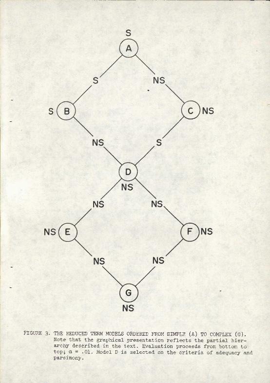
FIGURE 3. THE REDUCED TERM MODELS ORDERED FROM SIMPLE (A) TO COMPLEX (G). Note that the graphical presentation reflects the partial hierarchy described in the text. Evaluation proceeds from bottom to top; a = .01. Model D is selected on the criteria of adequacy and parsimony.

(56)

the extent to which the original cobble was modified to conform to a culturally-defined ideal. One would expect these variables to be correlated with sites as the manufacturinq process for picks was essentially the same across all Asturian sites (Clark 1971a:268,269). In short, the (ST) interaction might reflect human selection for a natural dimension; the (SDWL) interaction might reflect the imposition of technological attributes on a natural object. Taken toqcther, the two interactions adequately describe variation a'^ong the Asturian picks used in this example. Whether these same interactions would be isolated using different samples re-iains to be determined.

Summary

A method for analyzing data cast into continaency table format is presented. A series of models in the form of linear equations ordered in a hierarchy express relationships suspected eunong the variables selected for evaluation. Marginal totals corresponding to terms in the models are used to generate expected cell values; expected and observed cell values are ccmpared using a X distributed statistic called the loo likelihood ratio (log > ). Models are evaluated on the criteria of adequacy and parsimony; a "best" model is isolated. The "best" model is the simplest model which adequately describes the pattern of variation in the data. A simple example using archaeological data is presented to illustrate the approach.

Acknowledgements

I wish to express my sincere gratitude to Mr. T.P. Muller, the statistical consultant for the Department of Anthropology, University of Chicago, for invaluable assistance rendered during the planning and execution phases of the various techniques described in this paper. Without his help, and direction to pertinent source material, this paper would probably never have been written. The author, however, is solely responsible for overall content and for any factual or conceptual errors which the manuscript might contain. I also acknowledqe the assistance of various members of the Department of Anthropoloqy, Arizona State University, who read and criticized the manuscript at various stages in its development. Especially helpful were P.R. Fish, L.D. Smith, B. Domeier, B.L. Stark and J.D. Cadien.

(57)

REFERENCES CITED

Azoury, I. & Hodson, F.R.

1973

Comparing Paleolithic Assemblages: K'sar Akil, a case study. WORLD ARCHAEOLOGY 4:292-306.

Clark, G.A. 1971a-

1971b-

The Asturian of Cantabria: A re-evaluation. Unpublished Ph.D. Dissertation, Department of Anthropology, University of Chicago.

The Asturian of Cantabria: Subsistence Base and the Evidence for Post-Pleistocene Climatic Shifts. AMERICAN ANTHROPOLOGIST 73 (5): 1244-1257.

Fienberg, S. 1970

Goodman, L.A. 1968

1969

1970

The Analysis of Multidimensional Contingency Tables. ECOLOGY 51: 419-433.

The Analysis of Cross-classified Data: Independence, Quasi-Independence and Interactions in contingency tables with or without missing entries. JOURNAL OF THE AMERICAN STATISTICAL ASSOCIATION 63:1091-1131.

2 On Partitioning X and Detecting Partial Association in Three-way contingency tables. JOURNAL OF THE ROYAL STATISTICAL SOCIETY 31:486-498.

The Multivariate Analysis of Quantitative Data: Interactions among multiple classifications. JOURNAL OF THE AMERICAN STATISTICAL ASSOCIATION 65: 226-256.

Hodson, F.R. Cluster Analysis and Archaeology: some New 1970 Developments and Applications. WORLD ARCHAEOLOGY

299-320.

McNutt, C.H. On the Methodological Validity of Frequency 1973 Seriation. AMERICAN ANTIQUITY 38:45-60.

Muller, T.P. & Analysis of Contingency Table Data on Torus Mayhall, J. mandibularis using a Log Linear Model. AMERICAN

1971 JOURNAL OF PHYSICAL ANTHROPOLOGY 34:149-153.

Redman, C.L. Multistage Fieldwork and Analytical Techniques. 1973 AMERICAN ANTIQUITY 38:61-7 9.

Siegal, S. NON-PARAMETRIC STATISTICS FOR THE BEHAVIORAL 1956 SCIENCES. International Student Edition, pp. 42-47,

104-111, 175-179. McGraw Hill and Kogakusha. New York and Tokyo.

Vega del Sella,El Asturiense: Nueva Industria pre-neolitica. el Conde de la.COMISION DE INVESTIGACIONES PALEONTOLOGICAS Y

1923 PREHISTORICAS, MEMORIA NUM. 3 2 (Serie prehistorica Num. 27). Museo Nacional de Ciencias Naturales, Madrid.

(58)

Wallis. W.A. & STATISTICS: A NEW APPROACH. The Free Press, Roberts, H.V. New York.

1967

Weiss, K.A. Demographic Models for Anthropology. MEMOIRS 1973 OF THE SOCIETY FOR AMERICAN ARCHAEOLOGY No. 27.

Washington.

(47) on the analysis of multidimensional contingency table...

Documents