Local Volatility &

Heston Model

Master Dissertation By : Nishi Kanta Barnwal

2

Acknowledgement I would like to give my sincere thanks to all my colleagues at Natixis Asset Management, the company where I carried my internship to complete my studies, for their availability, support and confidence they have given me. I want to thank my Manager Samir Nait-Bachir, for giving me this great opportunity of working in this department. I would particularly like to thank Olivier Furet , structurer and quantitative analyst, for giving his invaluable time, assistance and knowledge to me in everyday work . Also a big thanks to him for his patience for me while teaching theory and application of various models and tools. I want to thank Laurent Eisenzimmer, Stephanie Ridon, Oumar Diawara, Ronan Juhé, Xie Yufeng for their availability and explanation of my doubts.

3

Contents Introduction 4 I Natixis Asset Management Company 4 II Structured products & shareholder funds department 6 1.Structuring team 6 2.Shareholder team 7 3.Portfolio team 7 Structuring Equation 8 III Quantitative Team 9 1.Lexifi 9 2.Bloomberg 10 3.Price-IT 10 IV Dividend Yield 11 1.From put/call parity 11 2.From Bloomberg and BNP Forward Curve 12 3.Seasonality Impact on Dividend 13 V BRIC 15 Introduction 15 Volatility Calculation 15 VI Equity Model in Lexifi 17 1.Local Volatility 17 2.Heston Model 18 VII Product 20 1.Vanilla Option 20 2.Exotic Options 20 2.1.Barrier Options 20 2.2.Forward –Start Option 21 2.3.Napoleon Option 22 VIII Monte Carlo Simulation 24 Conclusion 25

4

Introduction I spent 6 month working for two departments of Natixis Asset Management, Structured products & shareholder funds department where I realized quantitative analysis and the Marketing department , where I did statistical analysis on performance of old and closed Formula Funds.

I. NATIXIS Asset Management Company

Natixis Asset Management is one of Europe’s leading asset managers with 304 billion euros in assets under management. It offers a wide range of effective management solutions, based on extensive expertise in european and specialized asset management. Natixis Asset Management provides services to a diverse client base:

• Institutional investors, • Large companies, • Distributors, • Banque Populaire and Caisse d’Epargne clients.

Structured Products With euro11,67 billion in assets under management, Natixis Asset Management is the second-largest player in France in structured funds distributed to retail investors and ranks 6th in Europe in terms of assets managed. Its offer of structured products includes structuring and management of formula funds and actively managed capital-protected funds, or CPPI (constant Proportion Portfolio Insurance). !

!

!

!

!

!

!

5

!

!

!

"#$%&'()*!(+!,-.!/0!%11$2!34%11!!!

!

!!

!

!

!

"#$%&'()*!(+!,-.!/0!345$*2!3%2$6(#0!!!

!

!

6

Flexible and innovative Solutions Drawing on their experience with the Group’s distribution networks (Banques Populaires, Caisses d’Epargne) and external distributors, the investment teams have developed a wide range of formula funds. Numerous parameters are applied in designing these offers: structure engineering, level of protection (total/partial), leverage, asset selection, optimization of derivatives.

Furthermore, Natixis Asset Management also proposes active management with protected capital (or CPPI investment management) which has several advantages:

• indexation to virtually all the performance drivers available in the markets ; • partial and constant capital guarantee ; • gradual lock-in of gains ; • And the possibility for the investor to enter or exit the fund at any time.

Support that extends beyond product design

Natixis Asset Management’s Structured Products team (investment and support teams) supports distributors and investors throughout the product’s life:

• “ready-to-use solutions”: tailor-made design, legal and regulatory assistance, relations with counterparties ;

• research for best market conditions at launch of the fund (price, market understanding, transparency) and rigorous daily monitoring throughout the fund’s life ;

• Assistance in designing marketing tools.

II. Structured products & shareholder funds department:

The department consists of three teams. I worked for Quantitative team of structuring team.

1. Structuring team:

• The main task of the Structurer is to design the formula funds for retail customer which is the main and big business along with Developing private banking customer (funds).

• Developing automatable algorithm for managing funds. • Manage structured EMTN (Euro Medium Term Note) funds for Institutional

investor. Natixis Assurance is the main clients for this.

7

Insurance has to invest mainly in bonds but structured notes are good way of diversifying there investment and it allows to obtain alternative exposure like volatility or emerging markets without too much risk

2. Shareholder Team:

• Shareholder funds are design to promote investment of employees of a company in the shares of their own company. In these funds employees get the benefit of additional free shares.

• The majority of funds constitute the shares of the company • The company gives the benefit to the employee in the form of money and to avoid

the taxes on this money employee has to keep it in the funds for minimum 5 years in PEE (plan d’epargne enterprise)

• Developing a task to minimize the downside of the shares using put option or investing in volatility product ( variance swap or future on volatility index like eurostoxx volatility index V2X)

3. Portfolio team:

• Formula fund structuring: Formula fund is a fund in which you have a fixed maturity and based on the evolution of market and a defined formula it gives a contractual return. In retail funds the majority of formula funds have guaranteed capital and capital appreciation. For structuring these kind of funds NAM buy performance swap from investment banks. These performance swap contain three legs: Option, which gives capital appreciation to the fund; fees, which is asset manager wage; funding leg, which finance the two previous legs and has to be paid to investment bank. For paying this funding leg the fund has to invest in assets which produce sufficient return and obey to predefined constraints.

• Assurance Vie: It is a life insurance which present as a virtual product savings with tax benefits of insurance. In this case funding leg is Euribor and the assets are certificates(floating rate notes) or traditional bonds which are lend in exchange of lending fees. (Repurchase agreement).

• PEA (Plan d’epargne en actions): The PEA is a kind of security account in French law which enjoys certain tax benefits. To be eligible for PEA 75% of fund value has to be invested in European shares for minimum 5 years. Historically the constraint was only imposed in French shares. This is the reason why most of the PEA formula funds are structured with assets invested in CAC40.

8

Structuring Equation:

Life insurance

Buy a performance swap + Buy certificates

=

Long Option (The formula)

Long Fees

Short Funding Euribor Leg

+

Long Capital

Long Euribor Leg

=

At maturity

Long Option + Long Capital

PEA

Buy a performance swap + Buy CAC40 shares

=

Long Option (The formula)

Long Fees

Short Total returns CAC 40

(Short Call +Long Put +Short dividend swap)

+

CAC40 shares

=

Long Option + Long Capital

9

The portfolio manages the assets, to replicate the CAC40 performance or manage bond for paying the funding leg. Bonds for life insurance either hold to maturity or pension. It is a passive investment process without needing a market view.

III. Quantitative Team:

The tasks of quantitative team are:

• Price the derivative hold by the funds and produced by the department (particularly the performance swap). This help to negotiate the trading price.

• Every time the NAV (Daily or weekly or biweekly) has to be published, we have to calculate the performance swap value for challenging the prices sent by the counterparty (The one used in the NAV valuation process). If we disagree, we ask an audit of the counterparty price and revaluation.

• Define best practices of pricing according to pay off. • Check model implementation. • To develop analysis tool for choosing investment in structured product through

Risk return analysis

1. Backtesting of formulas 2. Monte Carlo simulation

• To check that the formula can be bought. • Performance swap value has to be zero according to the level of fees and

funding. It means that if the funding and the fees are fixed we have to solve an equation on option parameter definition

For this purpose (pricing and analysis) the quantitative team uses the following softwares:

1. Lexifi: It is the booking reference system for derivative products of the department. A system developed by a French company but because of its importance, the structuring department participates actively in its designing. It is a generic booking system (allow to book a very wide range of payoff) based on a language which is dedicated for describing financial contracts. This flexibility is very important for the structuring team because of the investment process which is focused on exotic products.

Core business of the system is booking flexibility. Pricing functionalities mainly for equity and interest rate derivatives have been developed recently. The quantitative team is focusing on improvement of the pricing models of this systems; Proposals from NAM (and other clients as well) are analysed by Lexifi Company and very often followed with new release which includes the suitable models.

A part of my job was to validate that the pricing models in Lexifi were well implemented. For this purpose I used the 2 pricing system described below.

10

2. Bloomberg: This software is used to get the market data and also for Vanilla pricing.

3. Price IT: Price-IT is Excel based software that provides powerful tools for quantitative financial analysis. The pricing process is decomposed into 4 independent components:

1. Generic payoff with a cash flow based description language using a simple and intuitive syntax to describe virtually any payoff from the most vanilla to the most complex financial product.

2. A set of plug and play models that can price any payoff described with our generic pricing technology.

3. A set of generic numerical methods that encompasses Monte Carlo, American Monte Carlo, tree engine and PDE. These numerical methods can be used by any compatible model to make a numerical model.

4. Last, a generic calibration component that enables to describe the model parameters estimation procedure in a unified and generic way.

The pricing methodology is synthetically presented in the following figure:

Price-IT is used as a benchmark for testing Lexifi pricer.

11

IV. Dividend Yield Dividend yield is one of the important parameters used in pricing equity derivatives. Earlier the structuring team was using constant dividend for pricing options in Lexifi. This dividend yield was obtained through Bloomberg field. The main aim is to improve the pricing process by adding term structure on dividend yield. So we have three possibilities to obtain the term structure dividend yield:

1. From Put/Call Parity based on option Price from Bloomberg 2. Forward curve from Bloomberg or other contributor (like BNP) 3. From dividend future

The first 2 methods give good results contrary to the last one. This is caused by funding (repo) costs includes in the implied dividend yield estimated in the first 2 methods. On account of this funding cost, the dividend future is bias.

1. From Put/Call Parity: put-call parity defines a relationship between the

price of a call option and a put option, both with the identical strike price and expiry. To derive the put-call parity relationship, the assumption is that the options are not exercised before expiration day, which necessarily applies to European options. Good estimation of this parameter depends upon the quality of option price source (synchronisation of put and call price, liquidity of the option). This is not guaranteed for the long dated maturity.

The formula for dividend yield is given by: Ln[S/(C-P+K*DF)]/(t-T)/365 Where, S is the spot value C is the call price P is the put price K is the strike DF is the discount Factor t is the different maturity T is the start date

12

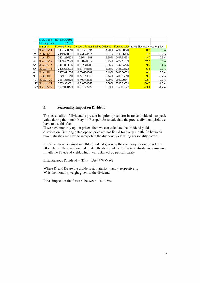
2. From Bloomberg and BNP Forward Curve: Using Bloomberg Future curve we have calculated implied dividend. The formula is given by:

Ln(S/Forward Value*DF)/(t-T)/365 In case of forward curve from Bloomberg and BNP, option price used in the forward calculation are supposed to be controlled. So there is no problem of long maturity option dividend yield estimation. Also we have compared Forward values obtained using different method, which includes Bloomberg forward curve, forward value using Future Dividend, BNP forward curve

13

3. Seasonality Impact on Dividend: The seasonality of dividend is present in option prices (for instance dividend has peak value during the month May, in Europe). So to calculate the precise dividend yield we have to use this fact. If we have monthly option prices, then we can calculate the dividend yield distribution. But long dated option price are not liquid for every month. So between two maturities we have to interpolate the dividend yield using seasonality pattern. In this we have obtained monthly dividend given by the company for one year from Bloomberg. Then we have calculated the dividend for different maturity and compared it with the Dividend yield, which was obtained by put call parity. Instantaneous Dividend = (D2t2 – D1t1)* Wi/!Wi

Where D2 and D1 are the dividend at maturity t2 and t1 respectively. Wi is the monthly weight given to the dividend. It has impact on the forward between 1% to 2%.

14

15

V. BRIC (Brazil Russia India China) Introduction The S&P BRIC 40 index is a basket of 40 leading securities, representing the largest and most liquid companies in Brazil, Russia, India and China (BRIC). All constituent companies are members of the S&P/IFC Investable index series that meet the requirements of all securities with a float adjusted market capitalization of US$ 1 billion and a minimum US$ 5 million average 3 month daily value traded prior to the selection date. Finally, the remaining securities are sorted in decreasing order of their float adjusted market cap and the top 40 become index members. The index is reviewed and rebalanced once a year, at which time new constituents may be added or deleted. In addition, a mid-year review is carried out to ensure the index’s representation is current and up to date. A full rebalance will be effective only if 3 of the biggest 30 stocks from the eligible universe are not in the index at the mid-year review. Through the year, companies may be deleted due to corporate events such as mergers, !acquisitions, takeovers, or delisting. Volatility calculation The list of 40 companies is obtained from S&P. Market caps and volatilities of these companies are obtained from Bloomberg to calculate the final volatility of the Index. The ticker used to obtain the volatility from Bloomberg is “Volatility_360_d_calc”(v), which is defined as the standard deviation of day to day logarithmic price changes. Previous day 360-day price volatility equals the annualized standard deviation of relative price change of the 360 most recent trading day’s closing price, expressed in a percentage for the day prior to the current. The Stock weight in Index is defined as the market cap of each company divide by the total market cap of the 40 companies. i.e. W = Market Cap (i)/ !Market Cap (i) i = 1 to 40 The Volatility is given by V = "((W*v)Transpose*Correlation Matrix*(W*v)) Correlation matrix is a matrix whose element in the i,j position is the correlation between ith and jth elements of a vector ( Here the vector is the list of companies).

16

The volatility obtained is 23.25%. and this volatility was matched with the short term volatility obtained from the contributor.

17

VI. Equity Model in Lexifi I have to validate the implementation of 2 equity pricing models in Lexifi, Local volatility model and Heston model. This validation is done through challenging Lexifi Valuation by Bloomberg and Pricing Partners.

1. Local Volatility:

B. Dupire extended the the Black Scholes model in order to fit the smile observed on the market. In this model, the stock price follows the equation:

where # is the stock volatility. While in the Black Scholes setting the volatility was constant, observe that now the volatility is a surface: # is a function depending on the time t and St the instantaneous price of the stock at time t. Due to this dependency, this kind of models are also called local volatility models. In essence, B. Dupire has shown that the local volatility was almost an observable in the market, and that it verifies:

Calibration The only parameter to calibrate is the local volatility, which is obtained using the above formula. This formula can be handled numerically using finite difference method, or using some kind of smoothed interpolation. Advantages: It fits the smile observed on the market, and for that reason this model is widely used in the financial industry. Another remarkable characteristic is that it maintains the completeness of market, which is the property that an option can be replicated via a self-financing trading strategy; a complete model has a unique equivalent martingale measure under which options can be priced. Stated more intuitively, within a complete market, for every possible state of the world (or outcome) there exist a security on the market. Limitations: Even if the local volatility model was designed to fit the smile, it fails to model accurately the forward volatility and is inappropriate for very short dated options, where the underlying can jump. Lexifi has various way of calculating local volatility. The analysis is limited to the Direct fitting and Gatheral direct smile:

18

Direct Fitting: The implied volatility surface is directly obtained by fitting market data quotes. In this setting, the surface is polynomial with degree in both maturity and strike. Recommended degrees are 2. This parameterization allows being very precise in retrieving vanilla option prices, But it is poor for extrapolating the smile. This model is called forward PDE in price IT. Direct Smile: For each maturity where multiple quotes are available, the implied volatility function is on a Gatheral function. A Gatheral function is defined as [sigma(k)2 = A + B * (Rho * (k - M) + sqrt{(k - M)2 + Sigma2}]. Quasi-explicit calibration is used which makes it quite fast and robust. Local volatility is then obtained by applying Dupire's formula with a linear interpolation of variance for maturity. This parameterization has a very good match to vanilla option price and allows an extrapolation of the smile which is consistent with stochastic volatility model. In Lexifi and price IT, it is possible to obtain the local volatility surface according to strike and maturity. Also it is possible to obtain the implied volatility matrix corresponding to the local volatility surface and compare it with initial volatility surface. An additional feature is the option price according to Black& Scholes formula versus the Monte Carlo pricing according to the local volatility model. (There could be convergence issues of Monte Carlo numerical methods).

2. Heston Model:

The first stochastic volatility model was proposed by Heston in 1993, who introduced an intuitive extension of the well known Black and Scholes modelization. He assumed that the spot price follows the diffusion:

that is, a process resembling geometric Brownian motion with a non-constant instantaneous variance V (t). Furthermore, he proposed that the variance is a CIR process, that is a mean reverting stochastic process of the form:

and allowed the two Brownian motions to be correlated with each other:

19

However, using the forward price of the underlying, the model becomes:

where F(t) is the forward at time t, and the five model’s parameters are:

1. the initial volatility:"V (0) 2. the long term variance: $ 3. the mean reversion of volatility: k 4. the volatility of volatility: % 5. the correlation & between the two Brownian processes W1 and W2

All these parameters can be calibrated.

Advantages: The model intuitively extends the Black and Scholes model, including it as a special case. The model is better used to price derivatives whose underlying is the spot itself, as it directly models St. Heston’s setting take into account non-lognormal distribution of the assets returns, leverage effect, important mean-reverting property of volatility and it remains analytically tractable. Limitations: The model has five parameters to calibrate. The volatility does not depend on the level of the spot, which may a drawback when the model is used to price products sensitive with respect to the spot of the underlying. Lexifi has Heston model without term structure. The 5 parameters estimation is done with a global optimization. Price IT has terms structure model but it is possible to use it with constant parameters. In Lexifi, the short term smile (1W option maturity) generates regularly a calibration problem. This is a limitation of Heston model to fit very steep smile corresponding to a premium against jump. So the short term smile has been suppressed of the calibration process.

20

VII. PRODUCT

1. Vanilla Option: An option contract with no special characteristics. It is either a call or a put, and has a standard expiry date and strike price. The contract contains no unusual provisions.

We did the pricing of this option in PriceIt and Lexifi softwares using local volatility model and Heston model calibration. For smoothning of volatility surface we used both forward PDE and Gatheral . But the results with the gatheral were better.

2. Exotic Options:

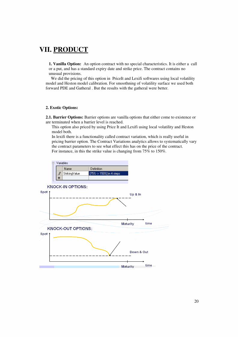
2.1. Barrier Options: Barrier options are vanilla options that either come to existence or are terminated when a barrier level is reached.

This option also priced by using Price It and Lexifi using local volatility and Heston model both. In lexifi there is a functionality called contract variation, which is really useful in pricing barrier option. The Contract Variations analytics allows to systematically vary the contract parameters to see what effect this has on the price of the contract. For instance, in this the strike value is changing from 75% to 150%. !!

21

2.2. Forward-start Option: Here we consider a one period forward call option that pays:

call Max(0, ST/St0 – K)

t : Today t0 : Forward start date t+ delta0 T : Maturity t+delta0+delta1 K Forward Strike

The forward smiles are more convex than today’s smile: since the price of a call option is an increasing and convex function of its implied volatility, uncertainty in the value of future implied volatility increases the option price.

22

2.3. Napoleon Option: Napoleon options are OTC-traded financial instruments that give their traders the opportunity to play with the volatility of a market. The main factors of the payoff of a Napoleon option are a fixed coupon and the worst returns of an index or equity over specified time periods.

23

24

VIII. Monte Carlo Simulation:

Monte Carlo methods are a class of computational algorithms that rely on repeated random sampling to compute their results. The main aim of this project is to find the best quadratic error and the best parameters of the Heston model. The algorithm begins with the assigning of number of iteration. We choose 10000 numbers of simulations. Then some initial and valid values are given to the parameters of Heston model along with the lower and upper boundary.

Then we enter in a loop of simulation in which every time all the parameters value are calculated using random number generator, within the boundary. After calculating a set of value of parameter of Heston model, we calculate the price of vanilla option using Addin of PriceIt software for different maturity and strike. Then we find the difference between this Heston model prices and vanilla option prices using Dupire model (which we calculated just once). Every time we compare the sum of differences with previous one and if it is smaller then we store the current parameters value in the best parameters cells otherwise the previous parameters value remain in the best parameters cells. At the end of this process we find the best quadratic error and best parameters of Heston model which gave this quadratic error. The formula for difference is defined as: (Option Price(using Heston Model) – Option Price(using Dupire model))2 *vega/ (Spotvalue)3 1%

After running the macro in excel, results obtained are:

25

Conclusion: Our main focus of study was pricing different options using local volatility and Heston model and then comparing it in Lexifi and Price-IT software’s. Advantage of Price-IT is there is Term Structure pricing where as there is no term structure option in Lexifi. But if we use a good calibrated model in Lexifi, then it gives good results. Stochastic Volatility models are useful because they explain in a self-Consistent way why it is that options with different strikes and expirations have different Black-Scholes implied volatilities- the “Volatility Smile”. But also, given the computational complexity of stochastic volatility models and the extreme difficulty of fitting parameters to the current prices of vanilla options, Local volatility is better and more consistent option for pricing.