5 mapping critical loads - · pdf filecalculating critical loads is to link, ... so-called...

The purpose of a model-based approach tocalculating critical loads is to link, via math-ematical equations, a chemical criterion(critical limit) with the maximumdeposition(s) ‘below which significant harm-ful effects on specified sensitive elements ofthe environment do not occur’, i.e. for whichthe criterion is not violated. In most casesthe ‘sensitive element of the environment’will be of a biological nature (e.g., the vitalityof a tree, the species composition of aheather ecosystem) and thus the criterionshould be a biological one. However, there isa dearth of simple yet reliable models thatadequately describe the whole chain fromdeposition to biological impact. Therefore,chemical criteria are used instead, and sim-ple chemical models are used to derive crit-ical loads. This simplifies the modellingprocess somewhat, but shifts the burden tofind, or derive, appropriate (soil) chemicalcriteria (and critical limits) with proven(empirical) relationships to biological effects.The choice of the critical limit is an importantstep in deriving a critical load, and much ofthe uncertainty in critical load calculationsstems from the uncertainty in the linkbetween (soil) chemistry and biologicalimpact.

In the following we consider only steady-state models, and concentrate on the so-called Simple Mass Balance (SMB) modelas the standard model for calculating criticalloads for terrestrial ecosystems under theLRTAP Convention (Sverdrup et al. 1990,Sverdrup and De Vries 1994). The SMBmodel is a single-layer model, i.e., the soil istreated as a single homogeneous compart-ment. Furthermore, it is assumed that thesoil depth is (at least) the depth of the rooting zone, which allows us to neglect thenutrient cycle and to deal with net growthuptake only. Additional simplifying assump-tions include:

• all evapotranspiration occurs on the topof the soil profile

• percolation is constant through the soil profile and occurs only vertically

• physico-chemical constants are assumed uniform throughout the whole soil profile

• internal fluxes (such as the weatheringrates, nitrogen immobilisation etc.) are independent of soil chemical conditions(such as pH)

Since the SMB model describes steady-state conditions, it requires long-term averages for input fluxes. Short-term variations – e.g., episodic, seasonal, inter-annual, due to harvest and as a resultof short-term natural perturbations – are notconsidered, but are assumed to be includedin the calculation of the long-term mean. Inthis context ‘long-term’ is defined as about100 years, i.e. at least one rotation period forforests. Ecosystem interactions andprocesses like competition, pests, herbivoreinfluences etc. are not considered in theSMB model. Although the SMB model is formulated for undisturbed (semi-natural)ecosystems, the effects of extensive management, such as grazing and the burning of moor, could be included.

Besides the single-layer SMB model, thereexist multi-layer steady-state models for calculating critical loads. Examples are theMACAL model (De Vries 1988) and the widely-used PROFILE model (Warfvinge andSverdrup 1992), which has at its core amodel for calculating weathering rates fromtotal mineral analyses. These models will notbe discussed here, and the interested readeris referred to the literature.

In the following sections we will derive theSMB model for critical loads of nutrientnitrogen (eutrophication) and critical loads of acidifying sulphur and nitrogen.

5 Mapping Critical Loads

Mapping Manual 2004 • Chapter V Mapping Critical Loads Page V - 10

5.3 Modelling Critical Loads for Terrestrial Ecosystems

5.3.1 Critical loads of nutrient nitrogen (eutrophication)

5.3.1.1 Model derivation

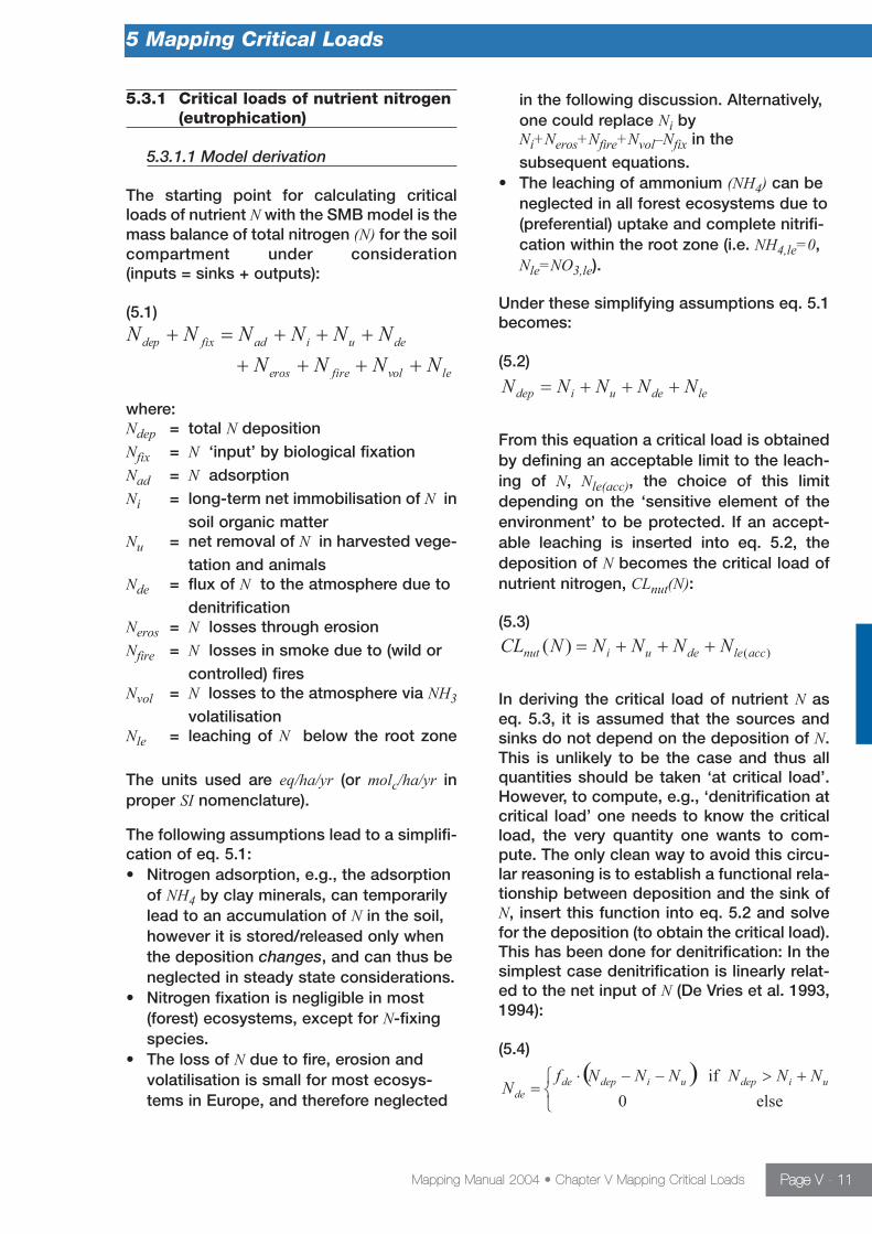
The starting point for calculating criticalloads of nutrient N with the SMB model is themass balance of total nitrogen (N) for the soilcompartment under consideration (inputs = sinks + outputs):

(5.1)

where:Ndep = total N depositionNfix = N ‘input’ by biological fixationNad = N adsorptionNi = long-term net immobilisation of N in

soil organic matterNu = net removal of N in harvested vege-

tation and animalsNde = flux of N to the atmosphere due to

denitrificationNeros = N losses through erosionNfire = N losses in smoke due to (wild or

controlled) firesNvol = N losses to the atmosphere via NH3

volatilisationNle = leaching of N below the root zone

The units used are eq/ha/yr (or molc/ha/yr inproper SI nomenclature).

The following assumptions lead to a simplifi-cation of eq. 5.1:• Nitrogen adsorption, e.g., the adsorption

of NH4 by clay minerals, can temporarily lead to an accumulation of N in the soil, however it is stored/released only when the deposition changes, and can thus be neglected in steady state considerations.

• Nitrogen fixation is negligible in most (forest) ecosystems, except for N-fixing species.

• The loss of N due to fire, erosion and volatilisation is small for most ecosys-tems in Europe, and therefore neglected

in the following discussion. Alternatively, one could replace Ni by Ni+Neros+Nfire+Nvol–Nfix in the subsequent equations.

• The leaching of ammonium (NH4) can be neglected in all forest ecosystems due to (preferential) uptake and complete nitrifi-cation within the root zone (i.e. NH4,le=0,Nle=NO3,le).

Under these simplifying assumptions eq. 5.1becomes:

(5.2)

From this equation a critical load is obtainedby defining an acceptable limit to the leach-ing of N, Nle(acc), the choice of this limitdepending on the ‘sensitive element of theenvironment’ to be protected. If an accept-able leaching is inserted into eq. 5.2, thedeposition of N becomes the critical load ofnutrient nitrogen, CLnut(N):

(5.3)

In deriving the critical load of nutrient N aseq. 5.3, it is assumed that the sources andsinks do not depend on the deposition of N.This is unlikely to be the case and thus allquantities should be taken ‘at critical load’.However, to compute, e.g., ‘denitrification atcritical load’ one needs to know the criticalload, the very quantity one wants to com-pute. The only clean way to avoid this circu-lar reasoning is to establish a functional rela-tionship between deposition and the sink ofN, insert this function into eq. 5.2 and solvefor the deposition (to obtain the critical load).This has been done for denitrification: In thesimplest case denitrification is linearly relat-ed to the net input of N (De Vries et al. 1993,1994):

(5.4)



where fde (0£ f de<1) is the so-called denitrifi-cation fraction, a site-specific quantity. Thisformulation implicitly assumes that immobil-isation and uptake are faster processes thandenitrification. Inserting this expression forNde into eq. 5.2 and solving for the depositionleads to the following expression for the critical load of nutrient N:

(5.5)

An alternative, non-linear, equation for thedeposition-dependence of denitrificationhas been proposed by Sverdrup and Ineson(1993) based on the Michaelis-Menten reaction mechanism and includes a depend-ence on soil moisture, pH and temperature.Also in this case CLnut(N) can be calculatedexplicitly, and for details the reader isreferred to Posch et al. (1993).

More generally, it would be desirable to havedeposition-dependent equations (models)for all N fluxes in the critical load equation.However, these either do not exist or are soinvolved that no (simple) explicit expressionfor CLnut(N) can be found. Although this doesnot matter in principle, it would reduce theappeal and widespread use of the criticalload concept. Therefore, when calculatingcritical loads from eq. 5.3 or eq. 5.5, the Nfluxes should be estimated as long-termaverages derived from conditions not influ-enced by elevated anthropogenic N inputs.

5.3.1.2 The acceptable leaching of nitrogen

The value set for the acceptable N leachingdepends on the ‘harmful effects’ that shouldbe avoided. In general, it is not the N leach-ing flux itself that is ‘harmful’, but the con-centration of N in the leaching flux. Theacceptable N leaching (in eq/ha/yr) is calcu-lated as:

(5.6)

where [N]acc is the acceptable N concentra-tion (eq/m3) and Q is the precipitation surplus(in m3/ha/yr). Values for acceptable Nconcentrations are given in Table 5.7.

To convert the values in Table 5.7 to eq/m3

divide them by 14. In general, the lowleaching values from the above table lead tocritical loads that are lower than empiricaldata on vegetation changes (e.g. Bobbink etal. 1998). It is the increase in N availabilitythrough enhanced N cycling that triggerschanges (Berendse et al. 1987).

An acceptable N leaching could also bederived with the objective to avoid N pollu-tion of groundwater using, e.g., the EC targetor limit value (25 and 50 mgN/L, resp.) asacceptable (but high!) concentration.



Table 5.7: Critical (acceptable) N concentrations in soil solution for calculating CLnut(N) updated 12.07.2007, see next page

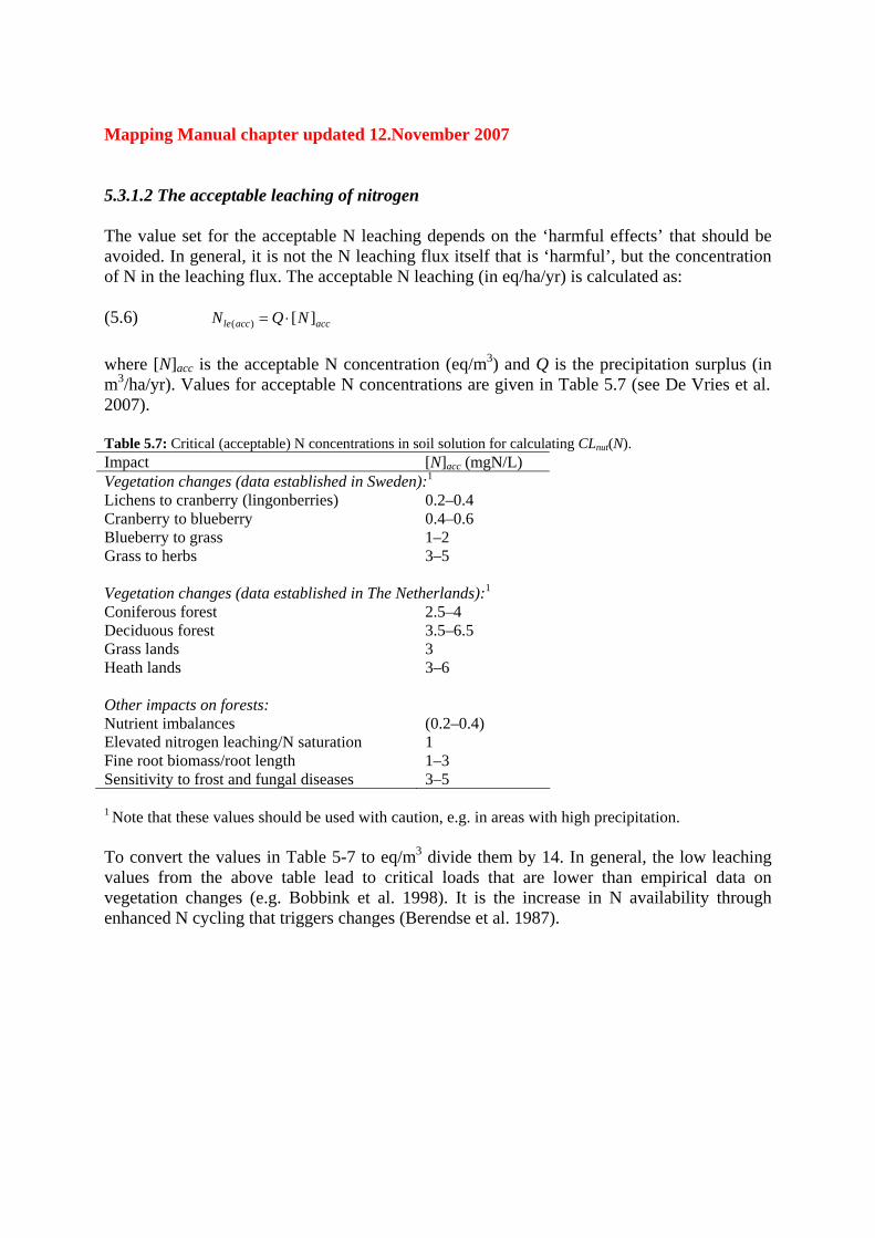
Mapping Manual chapter updated 12.November 2007 5.3.1.2 The acceptable leaching of nitrogen The value set for the acceptable N leaching depends on the ‘harmful effects’ that should be avoided. In general, it is not the N leaching flux itself that is ‘harmful’, but the concentration of N in the leaching flux. The acceptable N leaching (in eq/ha/yr) is calculated as: (5.6) accaccle NQN ][)( ⋅= where [N]acc is the acceptable N concentration (eq/m3) and Q is the precipitation surplus (in m3/ha/yr). Values for acceptable N concentrations are given in Table 5.7 (see De Vries et al. 2007). Table 5.7: Critical (acceptable) N concentrations in soil solution for calculating CLnut(N). Impact [N]acc (mgN/L) Vegetation changes (data established in Sweden):1

Lichens to cranberry (lingonberries) 0.2–0.4 Cranberry to blueberry 0.4–0.6 Blueberry to grass 1–2 Grass to herbs 3–5 Vegetation changes (data established in The Netherlands):1

Coniferous forest 2.5–4 Deciduous forest 3.5–6.5 Grass lands 3 Heath lands 3–6 Other impacts on forests: Nutrient imbalances (0.2–0.4) Elevated nitrogen leaching/N saturation 1 Fine root biomass/root length 1–3 Sensitivity to frost and fungal diseases 3–5

1 Note that these values should be used with caution, e.g. in areas with high precipitation. To convert the values in Table 5-7 to eq/m3 divide them by 14. In general, the low leaching values from the above table lead to critical loads that are lower than empirical data on vegetation changes (e.g. Bobbink et al. 1998). It is the increase in N availability through enhanced N cycling that triggers changes (Berendse et al. 1987).

5.3.1.3 Sources and derivation of input data

The obvious sources of input data for calcu-lating critical loads are measurements at thesite under consideration. However, in manycases these will not be available. A discus-sion on N sources and sinks can be found inHornung et al. (1995) and UNECE (1995).Some data sources and default values andprocedures to derive them are summarisedbelow.

Nitrogen immobilisation:Ni refers to the long-term net immobilisation(accumulation) of N in the root zone, i.e., thecontinuous build-up of stable C-N-com-pounds in (forest) soils. In other words, thisimmobilisation of N should not lead to signif-icant changes in the prevailing C/N ratio.This has to be distinguished from the highamounts of N accumulated in the soils over many years (decades) due to the increaseddeposition of N, leading to a decrease in theC/N ratio in the topsoil.

Using data from Swedish forest soil plots,Rosén et al. (1992) estimated the annual Nimmobilisation since the last glaciation at0.2–0.5 kgN/ha/yr (14.286–35714 eq/ha/yr).Considering that the immobilisation of N isprobably higher in warmer climates, valuesof up to 1 kgN/ha/yr (71.428 eq/ha/yr) could beused for Ni, without causing unsustainableaccumulation of N in the soil. It should bepointed out, however, that even higher values (closer to present-day immobilisationrates) have been used in critical load cal-culations. Although studies on the capacityof forests to absorb nitrogen have been carried out (see, e.g., Sogn et al. 1999), thereis no consensus yet on long-term sus-tainable immobilisation rates.

Nitrogen uptake:The uptake flux Nu equals the long-termaverage removal of N from the ecosystem.For unmanaged ecosystems (e.g., nationalparks) the long-term (steady-state) netuptake is basically zero whereas for managed forests it is the long-term netgrowth uptake. The harvesting practice is of

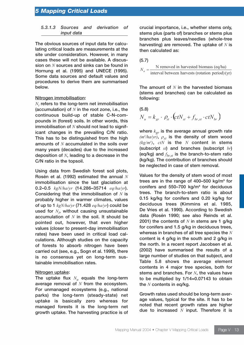
crucial importance, i.e., whether stems only,stems plus (parts of) branches or stems plusbranches plus leaves/needles (whole-treeharvesting) are removed. The uptake of N isthen calculated as:

(5.7)

The amount of N in the harvested biomass(stems and branches) can be calculated asfollowing:

(5.8)

where kgr is the average annual growth rate(m3/ha/yr), rst is the density of stem wood(kg/m3), ctN is the N content in stems (subscript st) and branches (subscript br)(eq/kg) and fbr,st is the branch-to-stem ratio(kg/kg). The contribution of branches shouldbe neglected in case of stem removal.

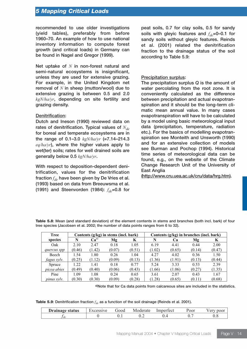
Values for the density of stem wood of mosttrees are in the range of 400–500 kg/m3 forconifers and 550–700 kg/m3 for deciduoustrees. The branch-to-stem ratio is about 0.15 kg/kg for conifers and 0.20 kg/kg fordeciduous trees (Kimmins et al. 1985, De Vries et al. 1990). According to Swedishdata (Rosén 1990; see also Reinds et al.2001) the contents of N in stems are 1 g/kgfor conifers and 1.5 g/kg in deciduous trees,whereas in branches of all tree species the Ncontent is 4 g/kg in the south and 2 g/kg inthe north. In a recent report Jacobsen et al.(2002) have summarised the results of alarge number of studies on that subject, andTable 5.8 shows the average element contents in 4 major tree species, both forstems and branches. For N, the values haveto be multiplied by 1/14=0.07143 to obtainthe N contents in eq/kg.

Growth rates used should be long-term aver-age values, typical for the site. It has to benoted that recent growth rates are higherdue to increased N input. Therefore it is



recommended to use older investigations(yield tables), preferably from before1960–70. An example of how to use nationalinventory information to compute forestgrowth (and critical loads) in Germany canbe found in Nagel and Gregor (1999).

Net uptake of N in non-forest natural andsemi-natural ecosystems is insignificant,unless they are used for extensive grazing.For example, in the United Kingdom netremoval of N in sheep (mutton/wool) due toextensive grazing is between 0.5 and 2.0kgN/ha/yr, depending on site fertility andgrazing density.

Denitrification:Dutch and Ineson (1990) reviewed data onrates of denitrification. Typical values of Ndefor boreal and temperate ecosystems are inthe range of 0.1–3.0 kgN/ha/yr (=7.14–214.3eq/ha/yr), where the higher values apply towet(ter) soils; rates for well drained soils aregenerally below 0.5 kgN/ha/yr.

With respect to deposition-dependent deni-trification, values for the denitrification fraction fde have been given by De Vries et al.(1993) based on data from Breeuwsma et al.(1991) and Steenvorden (1984): fde=0.8 for

peat soils, 0.7 for clay soils, 0.5 for sandysoils with gleyic features and fde=0–0.1 forsandy soils without gleyic features. Reindset al. (2001) related the denitrification fraction to the drainage status of the soilaccording to Table 5.9:

Precipitation surplus:The precipitation surplus Q is the amount ofwater percolating from the root zone. It isconveniently calculated as the differencebetween precipitation and actual evapotran-spiration and it should be the long-term cli-matic mean annual value. In many casesevapotranspiration will have to be calculatedby a model using basic meteorological inputdata (precipitation, temperature, radiationetc.). For the basics of modelling evapotran-spiration see Monteith and Unsworth (1990)and for an extensive collection of modelssee Burman and Pochop (1994). Historicaltime series of meteorological data can befound, e.g., on the website of the ClimateChange Research Unit of the University ofEast Anglia (http://www.cru.uea.ac.uk/cru/data/hrg.htm).



Table 5.9: Denitrification fraction fde as a function of the soil drainage (Reinds et al. 2001).

a)Note that for Ca data points from calcareous sites are included in the statistics.

Table 5.8: Mean (and standard deviation) of the element contents in stems and branches (both incl. bark) of fourtree species (Jacobsen et al. 2002; the number of data points ranges from 6 to 32).

Contents (g/kg) in stems (incl. bark) Contents (g/kg) in branches (incl. bark) Tree

species N Caa)

Mg K N Ca Mg K

2.10 2.47 0.18 1.05 6.19 4.41 0.44 2.00 Oak

quercus spp (0.46) (1.42) (0.07) (0.51) (1.02) (0.65) (0.14) (0.47)

Beech 1.54 1.80 0.26 1.04 4.27 4.02 0.36 1.50

fagus sylv. (0.25) (1.12) (0.09) (0.13) (1.36) (1.91) (0.13) (0.44)

Spruce 1.22 1.41 0.18 0.77 5.24 3.33 0.53 2.39

picea abies (0.49) (0.40) (0.06) (0.43) (1.66) (1.06) (0.27) (1.35)

Pine 1.09 1.08 0.24 0.65 3.61 2.07 0.43 1.67

pinus sylv. (0.30) (0.30) (0.09) (0.28) (1.28) (0.65) (0.11) (0.68)

5.3.2 Critical loads of acidity

5.3.2.1 Model derivation: the Simple Mass Balance (SMB) model

The starting point for deriving critical loadsof acidifying S and N for soils is the chargebalance of the ions in the soil leaching flux(De Vries 1991):

(5.9)

where the subscript le stands for leaching, Alstands for the sum of all positively chargedaluminium species, BC is the sum of basecations (BC=Ca+Mg+K+Na) and RCOO is thesum of organic anions. A leaching term isgiven by Xle=Q·[X], where [X] is the soil solu-tion concentration of ion X and Q is the precipitation surplus. All fluxes areexpressed in equivalents (moles of charge)per unit area and time (eq/ha/yr). The concen-trations of OH and CO3 are assumed zero,which is a reasonable assumption even forcalcareous soils. The leaching of AcidNeutralising Capacity (ANC) is defined as:

(5.10)

Combination with eq. 5.9 yields:

(5.11)

This shows the alternative definition of ANCas ‘sum of (base) cations minus strong acidanions’. For more detailed discussions onthe processes and concepts of (soil) chem-istry encountered in the context of acidifica-tion see, e.g., the books by Reuss andJohnson (1986) or Ulrich and Sumner (1991).

Chloride is assumed to be a tracer, i.e., thereare no sources or sinks of Cl within the soilcompartment, and chloride leaching is there-fore equal to the Cl deposition (subscriptdep):

(5.12)

In a steady-state situation the leaching ofbase cations has to be balanced by the netinput of base cations. Consequently the fol-lowing equation holds:

(5.13)

where the subscripts w and u stand forweathering and net growth uptake, i.e. thenet uptake by vegetation that is needed forlong-term average growth; Bc=Ca+Mg+K,reflecting the fact that Na is not taken up byvegetation. Base cation input by litterfall andBc removal by maintenance uptake (neededto re-supply base cations in leaves) is notconsidered here, assuming that both fluxesare equal (in a steady-state situation). Alsothe finite pool of base cations at theexchange sites (cation exchange capacity,CEC) is not considered. Although cationexchange might buffer incoming acidity fordecades, its influence is only a temporaryphenomenon, which cannot be taken intoaccount when considering long-termsteady-state conditions.

The leaching of sulphate and nitrate can belinked to the deposition of these compoundsby means of mass balances for S and N. ForS this reads (De Vries 1991):

(5.14)

where the subscripts ad, i, re and pr refer toadsorption, immobilisation, reduction andprecipitation, respectively. An overview ofsulphur cycling in forests by Johnson (1984)suggests that uptake, immobilisation andreduction of S have generally insignificant.Adsorption (and in some cases precipitationwith Al complexes) can temporarily lead to astrong accumulation of sulphate (Johnson et al. 1979, 1982). However, sulphate is onlystored or released at the adsorption complex when the input (deposition)changes, since the adsorbed S is assumed in



equilibrium with the soil solution S. Onlydynamic models can describe the time pattern of ad- and desorption of sulphate,but under steady-state conditions S ad- anddesorption and precipitation/mobilisationare not considered. Since sulphur is com-pletely oxidised in the soil profile, SO4,leequals Sle, and consequently:

(5.15)

For nitrogen, the mass balance in soil is (seeSection 5.3.1):

(5.16)

where the subscripts fix refers to fixation ofN, de to denitrification, and eros, fire and volto the loss of N due to erosion, forest firesand volatilisation, respectively. Ni is the long-term immobilisation of N in the root zone,and Nu the net growth uptake (see above).Furthermore, the leaching of NH4 can beneglected in almost all forest ecosystemsdue to (preferential) uptake and completenitrification within the root zone, i.e. NH4,le=0.Under these various assumptions eq. 5.16simplifies to:

(5.17)

Inserting eqs. 5.12, 5.13, 5.15 and 5.17 intoeq. 5.11 leads to the following simplifiedcharge balance for the soil compartment:

(5.18)

Strictly speaking, we should replace NO3,le inthe charge balance not by the right-handside of eq. 5.17, but bymax{Ndep–Ni–Nu–Nde,0}, since leaching cannot

become negative; and the same holds truefor base cations. However, this would lead tounwieldy critical load expressions; thereforewe go ahead with eq. 5.18, keeping this constraint in mind.

Since the aim of the LRTAP Convention is toreduce anthropogenic emissions of S and N,sea-salt derived sulphate should not be considered in the balance. To retain chargebalance, this is achieved by applying a sea-salt correction to sulphate, chloride andbase cations, using either Cl or Na as a tracer, whichever can be (safer) assumed tooriginale from sea-salts only. Denoting sea-salt corrected depositions with an asterisk, one has either Cl*

dep=0 or Na*dep=0

(and BC*dep=Bc*

dep), respectively. For procedures to compute sea-salt correcteddepositions, see Chapter 2.

For given values for the sources and sinks ofS, N and Bc, eq. 5.18 allows the calculation ofthe leaching of ANC, and thus assessment ofthe acidification status of the soil.Conversely, critical loads of S, CL(S), and N,CL(N), can be computed by defining a criticalANC leaching, ANCle,crit:

(5.19)

A so-called critical load of potential acidityhas earlier been defined (see Sverdrup et al.1990) as:

(5.20)

with Acpot = Sdep+Ndep–BC*dep+Cl*

dep. The term‘potential’ is used since NH3 is treated as(potential) acid due to the assumed complete nitrification. CL(Acpot) has beendefined to have no deposition terms in itsdefinition, since Bc and Cl deposition are notreally an ecosystem property and can (andoften do) change over time. However, sincethese depositions are partly of non-anthro-



pogenic origin (e.g., Saharan dust) and sincethey are not subject to emission reductionnegotiations, they are kept in the critical loaddefinition for convenience.

A further distinction has been made earlier(see, e.g., Sverdrup and De Vries 1994)between ‘land use acidity’ Bcu–Ni–Nu–Nde and‘soil acidity’ which is used to define a so-called critical load of (actual) acidity as:

(5.21)

The reason for making this distinction was toexclude all variables that may change in thelong term such as uptake of Bc and N, whichare influenced by forest management, and Nimmobilisation and denitrification, whichmay change due to changes in the hydrolog-ical regime. There are two problems with thisreasoning: (a) the remaining terms in eq. 5.21are also liable to change (e.g. ANC leachingdepends on precipitation surplus, see

below), and (b) uptake and other N process-es are a defining part of the ecosystem (veg-etation) itself. In other words, CL(A) may be acritical load of soil acidity, but it is rarely thesoil as such that is the ‘sensitive element’ tobe protected, but the vegetation growing onthat soil! Nevertheless, quantities such asCL(A) are computed and reported, and theycan have a role as useful short-hand notation for the variables involved.

Note that eq. 5.19 does not give a uniquecritical load for S or N. However, nitrogensinks cannot compensate incoming sulphuracidity, and therefore the maximum criticalload for sulphur is given by:

(5.22)

as long as N deposition is lower than all theN sinks, termed the minimum critical load ofN, i.e. as long as



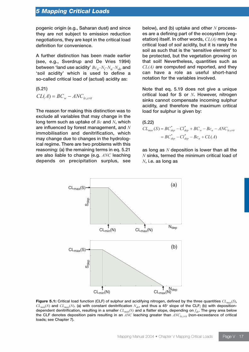
Figure 5.1: Critical load function (CLF) of sulphur and acidifying nitrogen, defined by the three quantities CLmax(S),CLmin(N) and CLmax(N). (a) with constant denitrification Nde, and thus a 45o slope of the CLF; (b) with deposition-dependent denitrification, resulting in a smaller CLmin(N) and a flatter slope, depending on fde. The grey area belowthe CLF denotes deposition pairs resulting in an ANC leaching greater than ANCle,crit (non-exceedance of criticalloads; see Chapter 7).

(5.23)

Finally, the maximum critical load of nitrogen(in the case of zero S deposition) is given by:

(5.24)

The three quantities CLmax(S), CLmin(N) andCLmax(N) define the critical load function(CLF; depicted in Figure 5.1a). Every deposi-tion pair (Ndep,Sdep) lying on the CLF are critical loads of acidifying S and N.

Deriving critical loads as above assumesthat the sources and sinks of N do notdepend on the N deposition. This is unlikelyto be true; and as in Section 5.3.1 we con-sider also the case of denitrification beinglinearly related to the net input of N.Substituting eq. 5.4 for Nde into the equationsabove results in the following expressionsfor CLmin(N) and CLmax(N):

(5.25)

and

(5.26)

where fde (0£ f de<1) is the denitrification fraction; CLmax(S) remains the same (eq.5.22). An example of a critical load functionwith fde>0 is shown in Figure 5.1b.

5.3.2.2 Chemical criteria and thecritical leaching of Acid Neutralising Capacity

The leaching of Acid Neutralising Capacity(ANC) is defined in eq. 5.10. In the simplestcase bicarbonate (HCO3) and organic anions(RCOO) are neglected since in general theydo not contribute significantly at low pH values. In this case the ANC leaching is givenby:

(5.27)

where Q is the precipitation surplus inm3/ha/yr (see Section 5.3.1.3 for data).

It is within the calculation of ANCle that thecritical chemical criterion for effects on thereceptor is set. Selecting the most appro-priate method of calculating ANCle is impor-tant, since the different methods may resultin very different critical loads. If, for the sameecosystem, critical loads are calculatedusing different criteria, the final critical loadis the minimum of all those calculated. Themain decision in setting the criterion willdepend on whether the receptor consideredis more sensitive to unfavourable pH condi-tions or to the toxic effects of aluminium.ANCle can then be calculated by either set-ting a hydrogen ion criterion (i.e., a criticalsoil solution pH) and calculating the criticalaluminium concentration, or vice versa.

The relationship between [H] and [Al] isdescribed by an (apparent) gibbsite equilib-rium:

(5.28)

where Kgibb is the gibbsite equilibrium constant (see below). Eq. 5.28 is used to calculate the (critical) Al concentration froma given proton concentration, or vice versa.

Different critical chemical criteria are listedbelow together with the equations for calcu-



lating ANCle,crit. In this context the readercould also consult the minutes of an ExpertWorkshop on ‘Chemical Criteria and CriticalLimits’ (UNECE 2001, Hall et al. 2001).

Aluminium criteria:Aluminium criteria are generally consideredmost appropriate for mineral soils with a loworganic matter content. Three commonlyused criteria are listed below.

(a) Critical aluminium concentration:Critical limits for Al have been suggested forforest soils, e.g., [Al]crit=0.2 eq/m3. These areespecially useful for drinking water (groundwater) protection, e.g., the EC drinking waterstandard for [Al] of maximally 0.2 mg/L(about 0.02 eq/m3). ANCle,crit can then be calculated as:

(5.29)

(b) Critical base cation to aluminium ratio:Most widely used for soils is the connectionbetween soil chemical status and plantresponse (damage to fine root) via a criticalmolar ratio of the concentrations of basecations (Bc=Ca+Mg+K) and Al in soil solution, denoted as (Bc/Al)crit. Values for alarge variety of plant species can be found inSverdrup and Warfvinge (1993). The mostcommonly used value is (Bc/Al)crit=1, thevalue for coniferous forests.

The critical Al leaching is calculated from theleaching of Bc (compare eq. 5.13):

(5.30)

The factor 1.5 arises from the conversion ofmols to equivalents (assuming K as divalent).Using eqs. 5.27 and 5.28, this yields for thecritical ANC leaching:

(5.31)

Note that the expression Bcle=Bcdep+Bcw–Bcuhas to be non-negative. In fact, it has beensuggested that it should be above a minimum leaching or, more precisely, there isa minimum concentration of base cations inthe leacheate, below which they cannot betaken up by vegetation, i.e., Bcle is set equalto max{0,Bcdep+Bcw–Bcu–Q·[Bc]min}, with[Bc]min in the order of 0.01eq/m3.

Alternatively, if considered more appropriate,a critical molar ratio of calcium to aluminiumin soil solution can be used, by replacing allthe Bc-terms in eq. 5.31 with Ca-terms.

(c) Critical aluminium mobilisation rate:Critical ANC leaching can also be calculatedusing a criterion to prevent the depletion ofsecondary Al phases and complexes whichmay cause structural changes in soils and afurther pH decline. Aluminium depletionoccurs when the acid deposition leads to anAl leaching in excess of the Al produced bythe weathering of primary minerals. Thus thecritical leaching of Al is given by:

(5.32)

where Alw is the weathering of Al from primary minerals (eq/ha/yr). The weatheringof Al can be related to the Bc weathering via:

(5.33)

where p is the stoichiometric ratio of Al to BCweathering in primary minerals (eq/eq), witha default value of p=2 for typical mineralogyof Northern European soils (range: 1.5–3.0).The critical leaching of ANC becomes then:



(5.34)

Hydrogen ion criteria:A proton criterion is generally recommendedfor soils with a high organic matter content.Two such criteria are listed below.

(a) Critical pH:A critical pH limit is set at a pH below whichthe receptor is adversely affected. Criticallimits have been suggested for forest soils,for example, pHcrit=4.0 (corresponding to[H]crit=0.1 eq/m3). ANCle,crit can then be calcu-lated as:

(5.35)

(b) Critical base cation to proton ratio:For organic soils which do not contain Al-(hydr)oxides (such as peat lands), it issuggested to use a critical molar basecation to proton ratio (Bc/H)crit. The criticalANC leaching is then given by (no Al leach-ing!):

(5.36)

where the factor 0.5 comes from convertingmols to equivalents. For organic soils theweathering in eq. 5.36 will probably be negligible (Bcw=0). Values suggested for(Bc/H)crit are expressed as multiples of(Bc/Al)crit, these multiples ranging from 0.3for deciduous trees and ground vegetationto 1 for spruce and pine (Sverdrup and Warfvinge 1993).

Critical base saturationBase saturation, i.e., the fraction of basecations at the cation exchange complex, isan indicator of the acidity status of a soil,and one may want to keep this pool above acertain level to avoid nutrient deficiencies.Thus a critical (acceptable, minimum) basesaturation could be chosen as a criterion forcalculating critical loads of acidity (see Hallet al. 2001, UNECE 2001).

To relate base saturation to ANC requires thedescription of the exchange of cationsbetween the exchange complex and the soilsolution. Two descriptions are the mostcommonly used in dynamic soil models: theGapon and the Gaines-Thomas exchangemodel. For a comparison between differentexchange models and the implications forthe relationship between base saturationand soil solution concentrations see Reuss(1983).As an example, we consider the descriptionof the exchange between H, Al andBc=Ca+Mg+K as implemented in the VerySimple Dynamic (VSD) as well as the SAFEmodel (see Posch et al. 2003a or Chapter 6on dynamic modelling). For both models thecritical concentration [H]crit can be found asa solution of an equation of the type:

(5.37)

where the coefficients A, B and the exponentp are given in Table 5.10.



Note: The generalised relationship [Al]=KAlox [H]a has been used (see below).

Table 5.10: Coefficients in eq. 5.37 for the Gapon and Gaines-Thomas exchange model.

In general, eq. 5.37 is non-linear and willhave to be solved numerically. Only for theGapon model and the gibbsite equilibrium(a=3, KAlox=Kgibb) it becomes a linear equa-tion with the solution:

(5.38)

where kHBc and kAlBc are the two (site-spe-cific) selectivity coefficients describingcation exchange and [Bc]=Bcle/Q as above.[Al]crit is then computed from the gibbsiteequilibrium (eq. 5.28) and from that the critical ANC leaching can be obtained via eq. 5.29. Values of selectivity coefficients fora range of (Dutch) soil types and combina-tions of exchangeable ions are given by De Vries and Posch (2003).

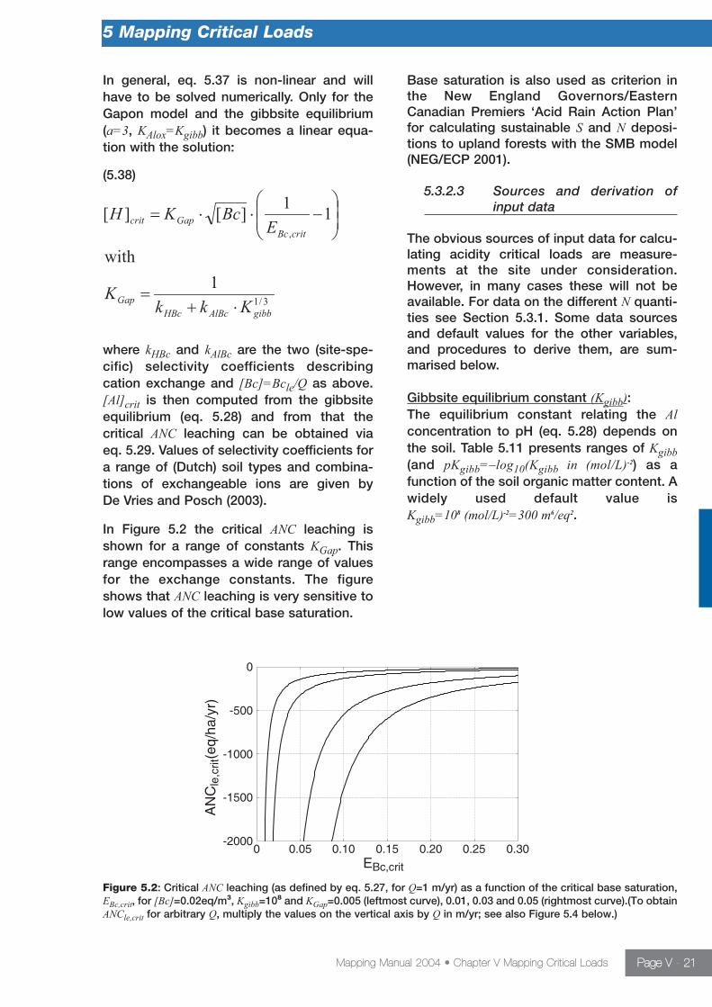
In Figure 5.2 the critical ANC leaching isshown for a range of constants KGap. Thisrange encompasses a wide range of valuesfor the exchange constants. The figureshows that ANC leaching is very sensitive tolow values of the critical base saturation.

Base saturation is also used as criterion inthe New England Governors/EasternCanadian Premiers ‘Acid Rain Action Plan’for calculating sustainable S and N deposi-tions to upland forests with the SMB model(NEG/ECP 2001).

5.3.2.3 Sources and derivation of input data

The obvious sources of input data for calcu-lating acidity critical loads are measure-ments at the site under consideration.However, in many cases these will not beavailable. For data on the different N quanti-ties see Section 5.3.1. Some data sourcesand default values for the other variables,and procedures to derive them, are sum-marised below.

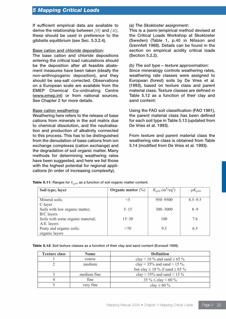
Gibbsite equilibrium constant (Kgibb):The equilibrium constant relating the Alconcentration to pH (eq. 5.28) depends onthe soil. Table 5.11 presents ranges of Kgibb(and pKgibb=–log10(Kgibb in (mol/L)-2) as a function of the soil organic matter content. Awidely used default value is Kgibb=108 (mol/L)-2=300 m6/eq2.



Figure 5.2: Critical ANC leaching (as defined by eq. 5.27, for Q=1 m/yr) as a function of the critical base saturation,EBc,crit, for [Bc]=0.02eq/m3, Kgibb=108 and KGap=0.005 (leftmost curve), 0.01, 0.03 and 0.05 (rightmost curve).(To obtainANCle,crit for arbitrary Q, multiply the values on the vertical axis by Q in m/yr; see also Figure 5.4 below.)

If sufficient empirical data are available toderive the relationship between [H] and [Al],these should be used in preference to thegibbsite equilibrium (see Sec. 5.3.2.4).

Base cation and chloride deposition:The base cation and chloride depositionsentering the critical load calculations shouldbe the deposition after all feasible abate-ment measures have been taken (ideally thenon-anthropogenic deposition), and theyshould be sea-salt corrected. Observationson a European scale are available from theEMEP Chemical Co-ordinating Centre(www.emep.int) or from national sources.See Chapter 2 for more details.

Base cation weathering:Weathering here refers to the release of basecations from minerals in the soil matrix dueto chemical dissolution, and the neutralisa-tion and production of alkalinity connectedto this process. This has to be distinguishedfrom the denudation of base cations from ionexchange complexes (cation exchange) andthe degradation of soil organic matter. Manymethods for determining weathering rateshave been suggested, and here we list thosewith the highest potential for regional appli-cations (in order of increasing complexity).

(a) The Skokloster assignment:This is a (semi-)empirical method devised atthe Critical Loads Workshop at Skokloster(Sweden) (Table 1, p.40 in Nilsson andGrennfelt 1988). Details can be found in thesection on empirical acidity critical loads(Section 5.2.2).

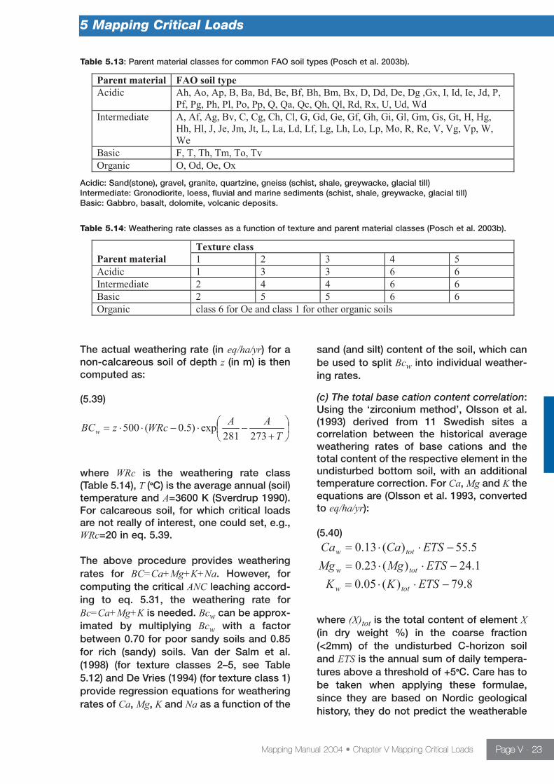
(b) The soil type – texture approximation:Since mineralogy controls weathering rates,weathering rate classes were assigned toEuropean (forest) soils by De Vries et al.(1993), based on texture class and parentmaterial class. Texture classes are defined inTable 5.12 as a function of their clay andsand content:

Using the FAO soil classification (FAO 1981),the parent material class has been definedfor each soil type in Table 5.13 (updated fromDe Vries et al. 1993).

From texture and parent material class theweathering rate class is obtained from Table5.14 (modified from De Vries et al. 1993).



Table 5.11: Ranges for Kgibb as a function of soil organic matter content.

Table 5.12: Soil texture classes as a function of their clay and sand content (Eurosoil 1999).

The actual weathering rate (in eq/ha/yr) for anon-calcareous soil of depth z (in m) is thencomputed as:

(5.39)

where WRc is the weathering rate class(Table 5.14), T (oC) is the average annual (soil)temperature and A=3600 K (Sverdrup 1990).For calcareous soil, for which critical loadsare not really of interest, one could set, e.g.,WRc=20 in eq. 5.39.

The above procedure provides weatheringrates for BC=Ca+Mg+K+Na. However, forcomputing the critical ANC leaching accord-ing to eq. 5.31, the weathering rate forBc=Ca+Mg+K is needed. Bcw can be approx-imated by multiplying Bcw with a factorbetween 0.70 for poor sandy soils and 0.85for rich (sandy) soils. Van der Salm et al.(1998) (for texture classes 2–5, see Table5.12) and De Vries (1994) (for texture class 1)provide regression equations for weatheringrates of Ca, Mg, K and Na as a function of the

sand (and silt) content of the soil, which canbe used to split Bcw into individual weather-ing rates.

(c) The total base cation content correlation:Using the ‘zirconium method’, Olsson et al.(1993) derived from 11 Swedish sites a correlation between the historical averageweathering rates of base cations and thetotal content of the respective element in theundisturbed bottom soil, with an additionaltemperature correction. For Ca, Mg and K theequations are (Olsson et al. 1993, convertedto eq/ha/yr):

(5.40)

where (X)tot is the total content of element X(in dry weight %) in the coarse fraction(<2mm) of the undisturbed C-horizon soiland ETS is the annual sum of daily tempera-tures above a threshold of +5oC. Care has tobe taken when applying these formulae,since they are based on Nordic geologicalhistory, they do not predict the weatherable



Table 5.13: Parent material classes for common FAO soil types (Posch et al. 2003b).

Acidic: Sand(stone), gravel, granite, quartzine, gneiss (schist, shale, greywacke, glacial till)Intermediate: Gronodiorite, loess, fluvial and marine sediments (schist, shale, greywacke, glacial till)Basic: Gabbro, basalt, dolomite, volcanic deposits.

Table 5.14: Weathering rate classes as a function of texture and parent material classes (Posch et al. 2003b).

soil depth, which was found to vary between20 and 200 cm in the field data, and theydon’t cover many soil types (mostly pod-zols).Using the part of the Swedish data (7-8 sitesdepending on the element, covering aweatherable depth of 20–100 cm), thismethod was adapted in Finland for estimat-ing weathering rates on a national scale(Johansson and Tarvainen 1997, Joki-Heiskala et al. 2003).

(d) The calculation of weathering rates withthe PROFILE model:Weathering rates can be computed with themulti-layer steady-state model PROFILE(Warfvinge and Sverdrup 1992 and 1995).Basic input data are the mineralogy of thesite or a total element analysis, from whichthe mineralogy is derived by a normativeprocedure. Generic weathering rates of eachmineral are modified by the concentration ofprotons, base cations, aluminium and organ-ic anions as well as the partial pressure ofCO2 and temperature. The total weatheringrate is proportional to soil depth and thewetted surface area of all minerals present.For the theoretical foundations of the weath-ering rate model see Sverdrup (1990). Forfurther information on the PROFILE modelsee www2.chemeng.lth.se.

(e) Other methods:Weathering rates can also be estimated frombudget studies of small catchments (see,e.g., Paces 1983). Be aware, however, thatbudget studies can easily overestimateweathering rates where there is significantcation release due to weathering of thebedrock. Other methods are listed anddescribed in Sverdrup et al. (1990).

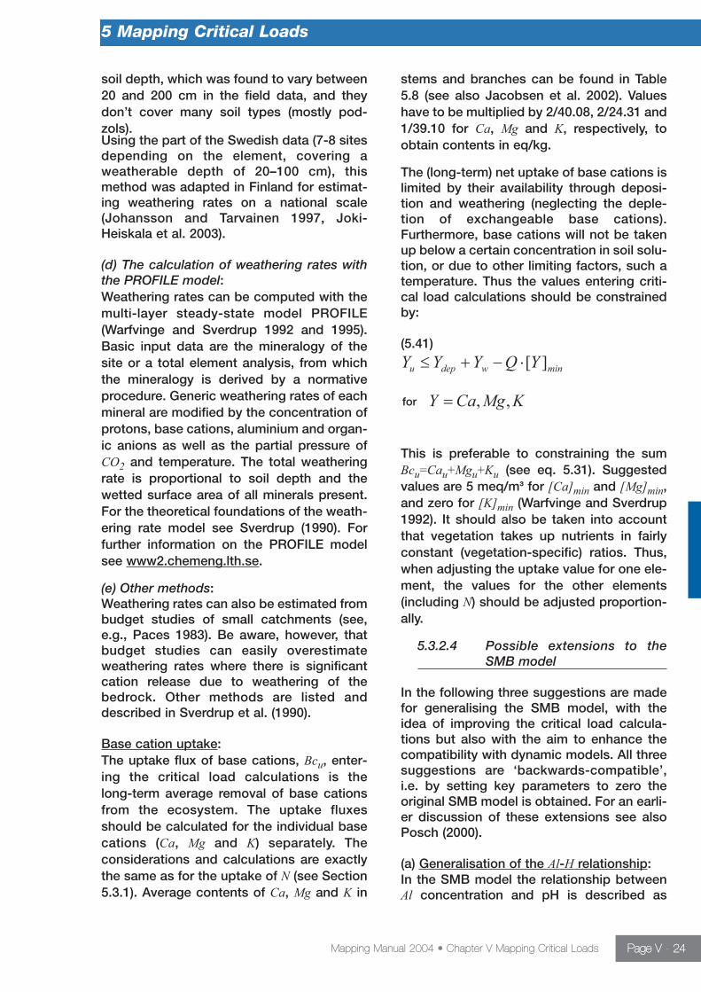
Base cation uptake:The uptake flux of base cations, Bcu, enter-ing the critical load calculations is the long-term average removal of base cationsfrom the ecosystem. The uptake fluxesshould be calculated for the individual basecations (Ca, Mg and K) separately. The considerations and calculations are exactlythe same as for the uptake of N (see Section5.3.1). Average contents of Ca, Mg and K in

stems and branches can be found in Table5.8 (see also Jacobsen et al. 2002). Valueshave to be multiplied by 2/40.08, 2/24.31 and1/39.10 for Ca, Mg and K, respectively, toobtain contents in eq/kg.

The (long-term) net uptake of base cations islimited by their availability through deposi-tion and weathering (neglecting the deple-tion of exchangeable base cations).Furthermore, base cations will not be takenup below a certain concentration in soil solu-tion, or due to other limiting factors, such atemperature. Thus the values entering criti-cal load calculations should be constrainedby:

(5.41)

This is preferable to constraining the sumBcu=Cau+Mgu+Ku (see eq. 5.31). Suggestedvalues are 5 meq/m3 for [Ca]min and [Mg]min,and zero for [K]min (Warfvinge and Sverdrup1992). It should also be taken into accountthat vegetation takes up nutrients in fairlyconstant (vegetation-specific) ratios. Thus,when adjusting the uptake value for one ele-ment, the values for the other elements(including N) should be adjusted proportion-ally.

5.3.2.4 Possible extensions to the SMB model

In the following three suggestions are madefor generalising the SMB model, with theidea of improving the critical load calcula-tions but also with the aim to enhance thecompatibility with dynamic models. All threesuggestions are ‘backwards-compatible’,i.e. by setting key parameters to zero theoriginal SMB model is obtained. For an earli-er discussion of these extensions see alsoPosch (2000).

(a) Generalisation of the Al-H relationship:In the SMB model the relationship betweenAl concentration and pH is described as



gibbsite equilibrium (see eq. 5.21). However,Al concentrations, especially in the topsoil,can be influenced by the complexation of Alwith organic matter (Cronan et al. 1986,Mulder and Stein 1994). Therefore, the gibb-site equilibrium in the SMB model could begeneralised by:

(5.42)

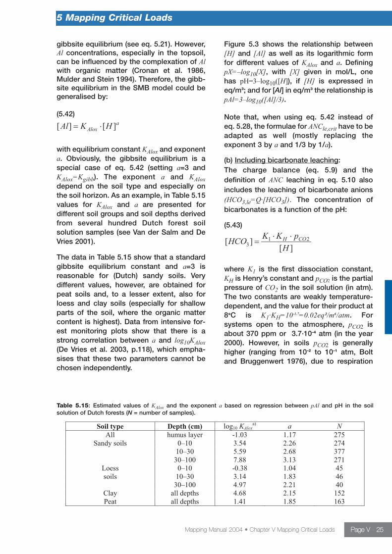
with equilibrium constant KAlox and exponenta. Obviously, the gibbsite equilibrium is aspecial case of eq. 5.42 (setting a=3 andKAlox=Kgibb). The exponent a and KAloxdepend on the soil type and especially onthe soil horizon. As an example, in Table 5.15values for KAlox and a are presented for different soil groups and soil depths derivedfrom several hundred Dutch forest soil solution samples (see Van der Salm and DeVries 2001).

The data in Table 5.15 show that a standardgibbsite equilibrium constant and a=3 is reasonable for (Dutch) sandy soils. Very different values, however, are obtained forpeat soils and, to a lesser extent, also forloess and clay soils (especially for shallowparts of the soil, where the organic mattercontent is highest). Data from intensive for-est monitoring plots show that there is astrong correlation between a and log10KAlox(De Vries et al. 2003, p.118), which empha-sises that these two parameters cannot bechosen independently.

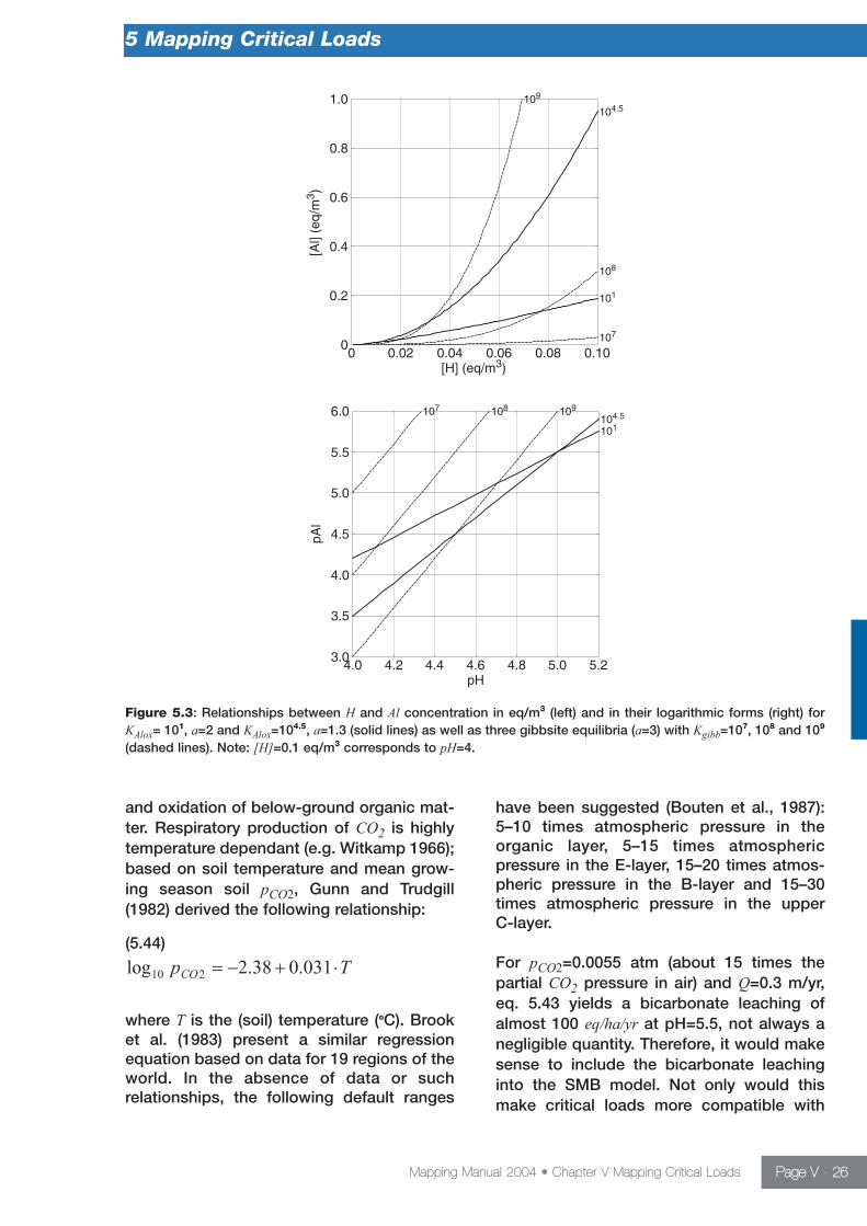
Figure 5.3 shows the relationship between[H] and [Al] as well as its logarithmic formfor different values of KAlox and a. DefiningpX=–log10[X], with [X] given in mol/L, onehas pH=3–log10([H]), if [H] is expressed ineq/m3; and for [Al] in eq/m3 the relationship ispAl=3–log10([Al]/3).

Note that, when using eq. 5.42 instead of eq. 5.28, the formulae for ANCle,crit have to beadapted as well (mostly replacing the exponent 3 by a and 1/3 by 1/a).

(b) Including bicarbonate leaching:The charge balance (eq. 5.9) and the definition of ANC leaching in eq. 5.10 alsoincludes the leaching of bicarbonate anions(HCO3,le=Q·[HCO3]). The concentration ofbicarbonates is a function of the pH:

(5.43)

where K1 is the first dissociation constant,KH is Henry’s constant and pCO2 is the partialpressure of CO2 in the soil solution (in atm).The two constants are weakly temperature-dependent, and the value for their product at8oC is K1·KH=10-1.7=0.02eq²/m6/atm. For systems open to the atmosphere, pCO2 isabout 370 ppm or 3.7·10–4 atm (in the year2000). However, in soils pCO2 is generallyhigher (ranging from 10–2 to 10–1 atm, Boltand Bruggenwert 1976), due to respiration



Table 5.15: Estimated values of KAlox and the exponent a based on regression between pAl and pH in the soil solution of Dutch forests (N = number of samples).

and oxidation of below-ground organic mat-ter. Respiratory production of CO2 is highlytemperature dependant (e.g. Witkamp 1966);based on soil temperature and mean grow-ing season soil pCO2, Gunn and Trudgill(1982) derived the following relationship:

(5.44)

where T is the (soil) temperature (oC). Brooket al. (1983) present a similar regressionequation based on data for 19 regions of theworld. In the absence of data or such relationships, the following default ranges

have been suggested (Bouten et al., 1987):5–10 times atmospheric pressure in theorganic layer, 5–15 times atmospheric pressure in the E-layer, 15–20 times atmos-pheric pressure in the B-layer and 15–30times atmospheric pressure in the upper C-layer.

For pCO2=0.0055 atm (about 15 times thepartial CO2 pressure in air) and Q=0.3 m/yr,eq. 5.43 yields a bicarbonate leaching ofalmost 100 eq/ha/yr at pH=5.5, not always anegligible quantity. Therefore, it would makesense to include the bicarbonate leachinginto the SMB model. Not only would thismake critical loads more compatible with



Figure 5.3: Relationships between H and Al concentration in eq/m3 (left) and in their logarithmic forms (right) forKAlox= 101, a=2 and KAlox=104.5, a=1.3 (solid lines) as well as three gibbsite equilibria (a=3) with Kgibb=107, 108 and 109

(dashed lines). Note: [H]=0.1 eq/m3 corresponds to pH=4.

steady-state solutions of dynamic models,but it is also the only way to allow the ANCleaching to obtain positive values! Eq. 5.27would than read:

(5.45)

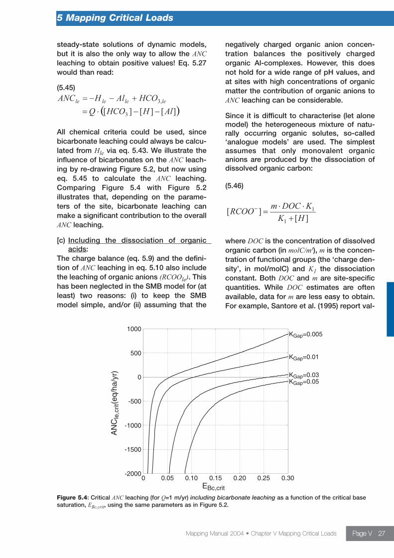
All chemical criteria could be used, sincebicarbonate leaching could always be calcu-lated from Hle via eq. 5.43. We illustrate theinfluence of bicarbonates on the ANC leach-ing by re-drawing Figure 5.2, but now usingeq. 5.45 to calculate the ANC leaching.Comparing Figure 5.4 with Figure 5.2 illustrates that, depending on the parame-ters of the site, bicarbonate leaching canmake a significant contribution to the overallANC leaching.

[c) Including the dissociation of organic acids:

The charge balance (eq. 5.9) and the defini-tion of ANC leaching in eq. 5.10 also includethe leaching of organic anions (RCOOle). Thishas been neglected in the SMB model for (atleast) two reasons: (i) to keep the SMBmodel simple, and/or (ii) assuming that the

negatively charged organic anion concen-tration balances the positively chargedorganic Al-complexes. However, this doesnot hold for a wide range of pH values, andat sites with high concentrations of organicmatter the contribution of organic anions toANC leaching can be considerable.

Since it is difficult to characterise (let alonemodel) the heterogeneous mixture of natu-rally occurring organic solutes, so-called‘analogue models’ are used. The simplestassumes that only monovalent organicanions are produced by the dissociation ofdissolved organic carbon:

(5.46)

where DOC is the concentration of dissolvedorganic carbon (in molC/m3), m is the concen-tration of functional groups (the ‘charge den-sity’, in mol/molC) and K1 the dissociationconstant. Both DOC and m are site-specificquantities. While DOC estimates are oftenavailable, data for m are less easy to obtain.For example, Santore et al. (1995) report val-



Figure 5.4: Critical ANC leaching (for Q=1 m/yr) including bicarbonate leaching as a function of the critical basesaturation, EBc,crit, using the same parameters as in Figure 5.2.

ues of m between 0.014 for topsoil samplesand 0.044 mol/molC for a B-horizon in theHubbard Brook experimental forest in NewHampshire.

Since a single value of K1 does not alwaysmodel the dissociation of organic acids satisfactorily, Oliver et al. (1983) havederived an empirical relationship between K1and pH:

(5.47)

with a=0.96, b=0.90 and c=0.039 (andm=0.120 mol/molC). Note that eq. 5.47 givesK1 in mol/L. In Figure 5.5 the fraction ofm·DOC dissociated as a function of pH isshown for the Oliver model and a mono-protic acid with a ‘widely-used’ valueof pK1=4.5.

Figure 5.5 shows that, depending on theamount of DOC, the contribution of organicanions to the ANC leaching, even at fairly lowpH, can be considerable.

Other models for the dissociation of organicacids have been suggested and are in use indynamic models, such as di- and tri-proticanalogue models (see, e.g., Driscoll et al.1994), or more detailed models of the speci-ation of humic substances, such as the

WHAM model (Tipping 1994). Any modelcould be used for the calculation of criticalloads as long as the dissociation dependsonly on [H], so that a critical leaching oforganic anions can be derived from [H]crit (or[Al]crit).



Figure 5.5: Fraction of organic acids (m DOC) dissociated as a function of pH for the Oliver model (solid line) andthe mono-protic model (eq.5.46) with pK1=4.5 (dashed line).

5 mapping critical loads - · pdf filecalculating critical loads is to link, ... so-called...

Documents