5. openness in goods and financial markets: the current ... · openness in goods and financial...

Fletcher School of Law and Diplomacy, Tufts University

5. Openness in Goods and Financial Markets: The Current Account, Exchange Rates and the International Monetary System

Macroeconomics

Prof. George Alogoskoufis

George Alogoskoufis, Macroeconomics, 2017-18

Open versus Closed EconomiesNational economies are interconnected through trade in goods and services, through migration flows and through international capital markets. We refer to such economies as open economies. In fact all economies are open to a significant degree. The only truly closed economy is the global economy.

Openness has three important dimensions:

1. Openness in goods markets—the ability of consumers and firms to choose between domestic goods and foreign goods. In no country is this choice completely free of restrictions: Even the countries most committed to free trade have tariffs—taxes on imported goods—and quotas— restrictions on the quantity of goods that can be imported—on at least some foreign goods. At the same time, in most countries, average tariffs are low and getting lower.

2. Openness in financial markets—the ability of financial investors to choose between domestic assets and foreign assets. Until relatively recently even some of the richest countries in the world, such as France and Italy, had capital controls—restrictions on the foreign assets their domestic residents could hold and the domestic assets foreigners could hold. These restrictions have largely disappeared, with the exception of China and other emerging economies. As a result, world financial markets are becoming more and more closely integrated.

3. Openness in factor markets—the ability of firms to choose where to locate production, and of workers to choose where to work. Here trends are also clear. Multinational companies operate plants in many countries and move their operations around the world to take advantage of low costs. Much of the debate about the North American Free Trade Agreement (NAFTA) signed in 1993 by the United States, Canada, and Mexico centered on how it would affect the relocation of U.S. firms to Mexico. Similar fears now center around China. In addition, immigration from low-wage countries, is a hot political issue in countries from Germany, France, the United Kingdom and other countries in the European Union, to the United States.

2


Openness, the Balance of Payments and Exchange Rates

An open economy can borrow or lend resources to the rest of the world. In contrast to a closed economy, domestic investment may thus differ from national savings. The difference determines the balance of payments.

In addition, transactions among open economies are in many currencies. The relative prices of those currencies, exchange rates, are constantly changing in the current system of floating exchange rates. However, many countries have adopted regimes of fixed or managed exchange rates.

The largest part of international transactions among open economies takes place through international financial and capital markets. These markets allow households and firms to exchange cash and securities (promises of future payment) in different currencies, allow countries to finance deficits in their balance of payments and firms to engage in foreign direct investment.

3


Openness in the Industrial EconomiesThe industrial economies are becoming increasingly open.

For example, in the United States, the average of imports and exports, which is a widely used measure of opennesss, was about 5% in 1960, versus about 15% now. Exports and imports have more than tripled relative to GDP not only in the USA but in almost all the industrial economies.

A better index of openness is the share of tradable goods and services to GDP. Tradable goods and services are those which compete with foreign goods and services in either domestic markets or foreign markets. Estimates for the share of tradable goods to GDP in the United States put it at around 60% of GDP.

In any case, the USA is a large and highly diversified economy, and this is the main reason behind its relatively low import and export ratio. Smaller and less diversified economies have higher openness ratios. In 2014, exports in the USA amounted to 13.5% of GDP, versus 17.7% in Japan, 28.3% in the United Kingdom and 45.7% in Germany. The Netherlands, a small open European economy, had an export ratio of 82.9% of GDP.

4


Imports and Exports in the United States

5

0.0%

2.0%

4.0%

6.0%

8.0%

10.0%

12.0%

14.0%

16.0%

18.0%

20.0% 19

48.01

1949

.02

1950

.03

1951

.04

1953

.01

1954

.02

1955

.03

1956

.04

1958

.01

1959

.02

1960

.03

1961

.04

1963

.01

1964

.02

1965

.03

1966

.04

1968

.01

1969

.02

1970

.03

1971

.04

1973

.01

1974

.02

1975

.03

1976

.04

1978

.01

1979

.02

1980

.03

1981

.04

1983

.01

1984

.02

1985

.03

1986

.04

1988

.01

1989

.02

1990

.03

1991

.04

1993

.01

1994

.02

1995

.03

1996

.04

1998

.01

1999

.02

2000

.03

2001

.04

2003

.01

2004

.02

2005

.03

2006

.04

2008

.01

2009

.02

2010

.03

2011

.04

2013

.01

2014

.02

2015

.03

2016

.04

Recessions ExportsofGoodsandServices(%ofGDP) ImportsofGoodsandServices(%ofGDP)


National Income Accounting in an Open Economy

❖ There are three main points that need to be clearly understood is relation to open economies:

❖ First, in an open economy domestic expenditure can differ from domestic output. Their difference determines the trade balance.

❖ Second, the relationship between the trade balance, the fiscal balance and the balance of private savings and investment.

❖ Thirdly, the important distinction between Gross Domestic Product (GDP) and Gross National Income (GNI or GNP).

6


The Relationship between Domestic Income and Expenditure in an Open Economy, and the Determination of the Trade Balance

Aggregate demand (D) for the Gross Domestic Product (Y) in an open economy is equal to the sum of private consumption (C), private investment (I), government expenditure (G) and exports (X), minus imports (M). This identity takes the form,

Y = D = C + I + G + ( X – M )

Aggregate Gross Domestic Expenditure, sometimes called absorption, which we shall now denote by Z, may differ from Gross Domestic Product (Y), as it is equal to

Z = C + I + G

It follows that,

Υ = Z + ( Χ – Μ )

The trade balance (or net exports NX), defined as exports minus exports, is thus equal to the difference between Gross Domestic Product and Gross Domestic Expenditure and is given by,

NX = X – M = Y – Z

7


The Trade Balance is a Macroeconomic Phenomenon

❖ The trade balance is merely the difference of gross domestic product and expenditure.

❖ This is a very important observation because it directs our attention to the macroeconomic nature of external imbalances.

❖ The adjustment of external imbalances requires measures to restore the relationship between domestic output and income and domestic expenditure.

❖ One can analyze this connection to an even greater depth by subtracting from both sides of the income and expenditure identity total taxes (net of transfers) T, and adding on both sides net income from the rest of the world R, defined as the income of domestic residents generated outside the country.

8


The Current Account of the Balance of Payments

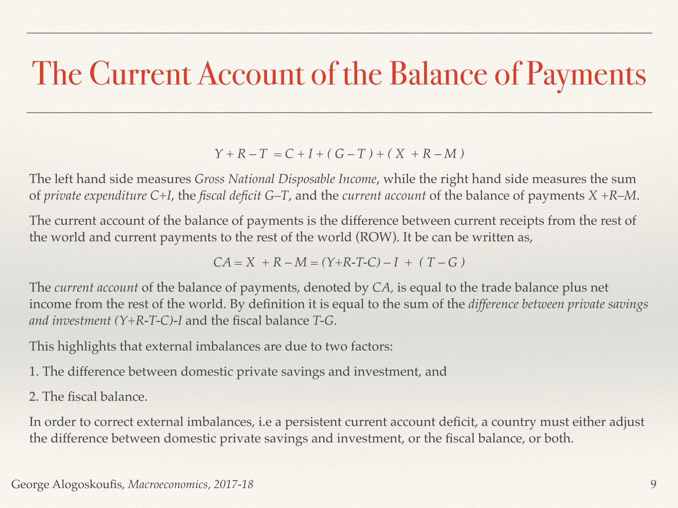
Y + R – T = C + I + ( G – T ) + ( X + R – M )

The left hand side measures Gross National Disposable Income, while the right hand side measures the sum of private expenditure C+I, the fiscal deficit G–T, and the current account of the balance of payments X +R–M.

The current account of the balance of payments is the difference between current receipts from the rest of the world and current payments to the rest of the world (ROW). It be can be written as,

CA = X + R – M = (Y+R-T-C) – I + ( T – G )

The current account of the balance of payments, denoted by CA, is equal to the trade balance plus net income from the rest of the world. By definition it is equal to the sum of the difference between private savings and investment (Y+R-T-C)-I and the fiscal balance T-G.

This highlights that external imbalances are due to two factors:

1. The difference between domestic private savings and investment, and

2. The fiscal balance.

In order to correct external imbalances, i.e a persistent current account deficit, a country must either adjust the difference between domestic private savings and investment, or the fiscal balance, or both.

9


The Current Account and the Capital Account

In absolute terms, the current account is equal to the capital account, i.e the net flows of assets, including money, in and out of the country.

When the current account is in surplus, the country spends less on goods and services from the rest of the world than the sum of its receipts from exports and its net income from the rest of the world. Thus, it accumulates assets vis-a-vis the rest of the world, and the capital account is in deficit.

If the current account is in deficit, the country spends more on goods and services from the rest of the world than the sum of its receipts from exports and its net income from the rest of the world. Therefore, the country has to import capital from the rest of the world, in order to finance this deficit. The capital account is thus in surplus, as there is a decumulation of assets vis-a-vis the rest of the world, or a buildup of external debt.

As we shall see soon, the method of financing current account imbalances has significant short term and long term implications.

10


The Current Account of the USA 1960-2016

11

-7.00

-6.00

-5.00

-4.00

-3.00

-2.00

-1.00

0.00

1.00

2.001960.01

1961.02

1962.03

1963.04

1965.01

1966.02

1967.03

1968.04

1970.01

1971.02

1972.03

1973.04

1975.01

1976.02

1977.03

1978.04

1980.01

1981.02

1982.03

1983.04

1985.01

1986.02

1987.03

1988.04

1990.01

1991.02

1992.03

1993.04

1995.01

1996.02

1997.03

1998.04

2000.01

2001.02

2002.03

2003.04

2005.01

2006.02

2007.03

2008.04

2010.01

2011.02

2012.03

2013.04

2015.01

2016.02

Current Account oftheUSA(%ofGDP)


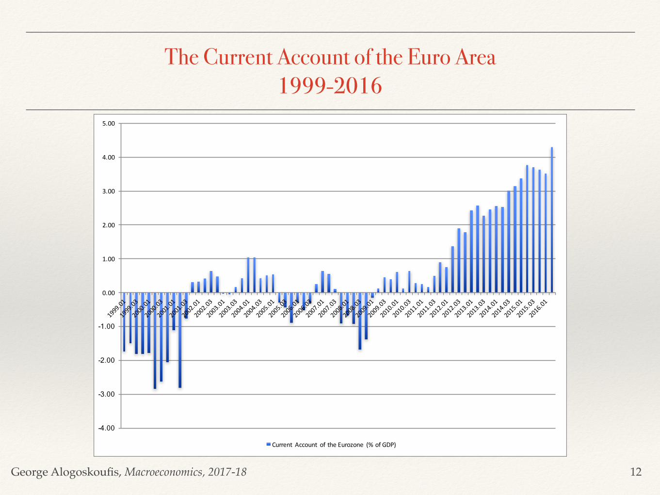
The Current Account of the Euro Area 1999-2016

12

-4.00

-3.00

-2.00

-1.00

0.00

1.00

2.00

3.00

4.00

5.00

Current Account oftheEurozone (%ofGDP)


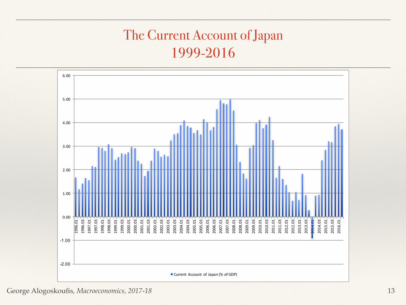
The Current Account of Japan 1999-2016

13

-2.00

-1.00

0.00

1.00

2.00

3.00

4.00

5.00

6.001996.01

1996.03

1997.01

1997.03

1998.01

1998.03

1999.01

1999.03

2000.01

2000.03

2001.01

2001.03

2002.01

2002.03

2003.01

2003.03

2004.01

2004.03

2005.01

2005.03

2006.01

2006.03

2007.01

2007.03

2008.01

2008.03

2009.01

2009.03

2010.01

2010.03

2011.01

2011.03

2012.01

2012.03

2013.01

2013.03

2014.01

2014.03

2015.01

2015.03

2016.01

Current Account ofJapan(%ofGDP)


Relationship between Gross Domestic Product (GDP) and Gross National Product (GNP)

❖ To the extent that a country has non zero net income from the rest of the world, we distinguish between Gross Domestic Product (GDP) and Gross National Product (GNP) or, equivalently, Gross National Income (GNI).

❖ GDP is the value of domestic production and income, and GNP (GNI) is the the total income of the country's inhabitants (domestic residents).

❖ Net income from the rest of the world can be either net income from capital (interest and dividends), or net income from labor (labor supply of domestic residents to the rest of the world).

❖ When we come to issues of asset or debt accumulation from the rest of the world, this distinction becomes central.

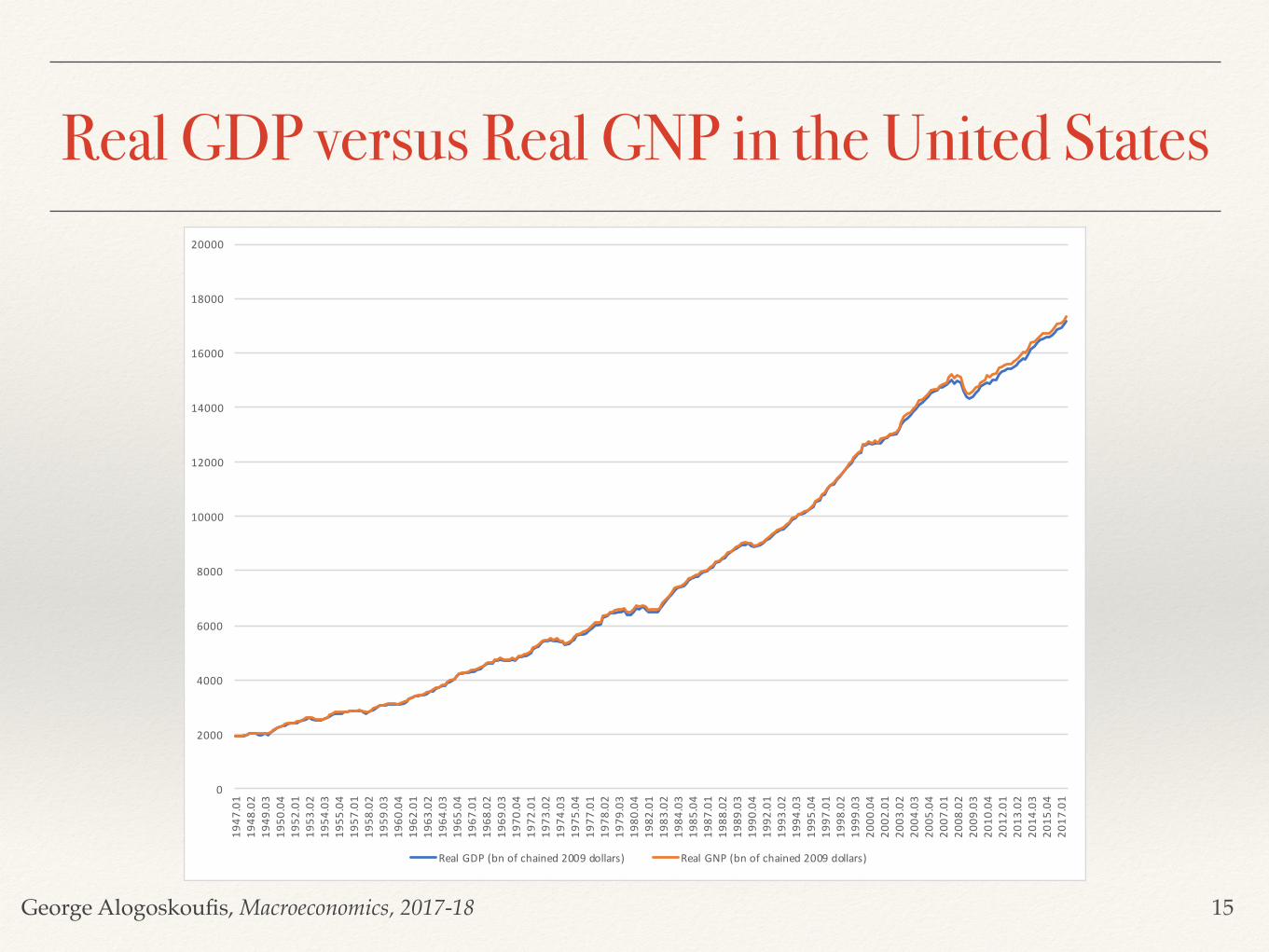
❖ The difference between real GDP and real GNP in the United States is about 1% of GDP. GNP is 1% higher than GDP because of the net income from US investments in the rest of the world.

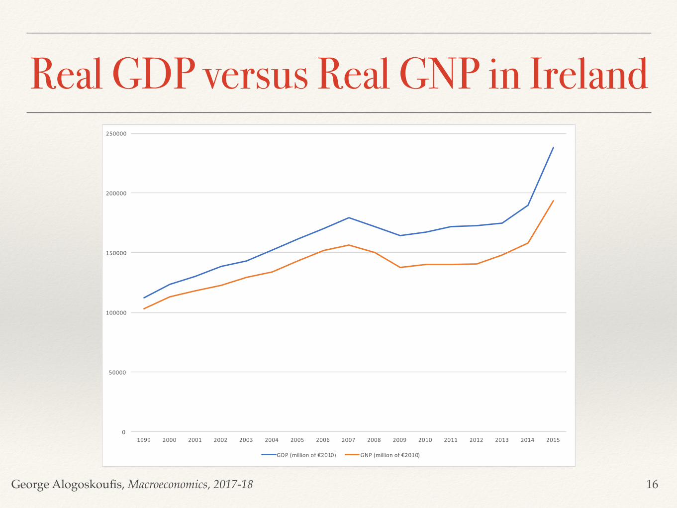
❖ However, the difference between real GDP and real GNP in Ireland, an economy which has received a lot of foreign direct investment, is about 19% of GDP. GNP is 19% lower than GDP because of the net income that is repatriated from Ireland to the rest of the world.

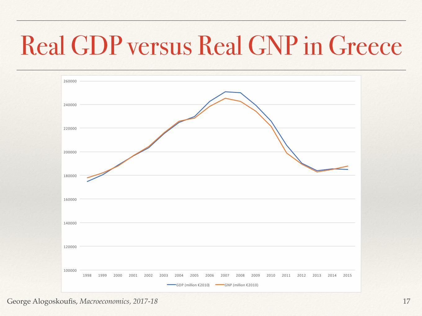
❖ The relationship between GDP and GNP can switch over time, as a result of accumulation of external imbalances. For example in Greece, in 1998, GNP was 2% higher than GDP, because of positive net income from the rest of the world (shipping). By the time of the crisis of 2010, GNP had become 2% lower than GDP, because of sustained current deficits, that had led to external debt accumulation, and interest payments to the rest of the world.

14


Real GDP versus Real GNP in the United States

15

0

2000

4000

6000

8000

10000

12000

14000

16000

18000

2000019

47.01

1948

.02

1949

.03

1950

.04

1952

.01

1953

.02

1954

.03

1955

.04

1957

.01

1958

.02

1959

.03

1960

.04

1962

.01

1963

.02

1964

.03

1965

.04

1967

.01

1968

.02

1969

.03

1970

.04

1972

.01

1973

.02

1974

.03

1975

.04

1977

.01

1978

.02

1979

.03

1980

.04

1982

.01

1983

.02

1984

.03

1985

.04

1987

.01

1988

.02

1989

.03

1990

.04

1992

.01

1993

.02

1994

.03

1995

.04

1997

.01

1998

.02

1999

.03

2000

.04

2002

.01

2003

.02

2004

.03

2005

.04

2007

.01

2008

.02

2009

.03

2010

.04

2012

.01

2013

.02

2014

.03

2015

.04

2017

.01

RealGDP(bnofchained2009dollars) RealGNP(bnofchained2009dollars)


Real GDP versus Real GNP in Ireland

16

0

50000

100000

150000

200000

250000

1999 2000 2001 2002 2003 2004 2005 2006 2007 2008 2009 2010 2011 2012 2013 2014 2015

GDP(millionof€2010) GNP(millionof€2010)


Real GDP versus Real GNP in Greece

17

100000

120000

140000

160000

180000

200000

220000

240000

260000

1998 1999 2000 2001 2002 2003 2004 2005 2006 2007 2008 2009 2010 2011 2012 2013 2014 2015

GDP(million€2010) GNP(million€2010)


The Choice between Domestic Goods and Foreign Goods

How does openness in goods markets force us to rethink the way we look at equilibrium in the goods market?

Until now, when we were thinking about consumers’ decisions in the goods market, we focused on their decision to save or to consume. When goods markets are open, domestic consumers face a second decision: whether to buy domestic goods or to buy foreign goods. Indeed, all buyers—including domestic and foreign firms and governments—face the same decision. This decision has a direct effect on domestic output: If buyers decide to buy more domestic goods, the demand for domestic goods increases, and so does domestic output. If they decide to buy more foreign goods, then foreign output increases instead of domestic output.

Central to this second decision (to buy domestic goods or foreign goods) is the price of domestic goods relative to foreign goods. We call this relative price the real exchange rate.

The real exchange rate is not directly observable, and you will not find it in the newspapers. What you will find in newspapers are nominal exchange rates, the relative prices of currencies. So we start by looking at nominal exchange rates and then see how we can use them to construct real exchange rates.

18


Nominal and Real Exchange RatesThe bilateral nominal exchange rate (S) is defined as the value of a country's currency in terms of another currency. We shall define it as units of foreign currency per unit of domestic currency. Thus, when the bilateral nominal exchange rate rises, we shall say that the domestic currency has appreciated, while when the bilateral nominal exchange rate falls, we shall say that the domestic currency has depreciated against the foreign currency.

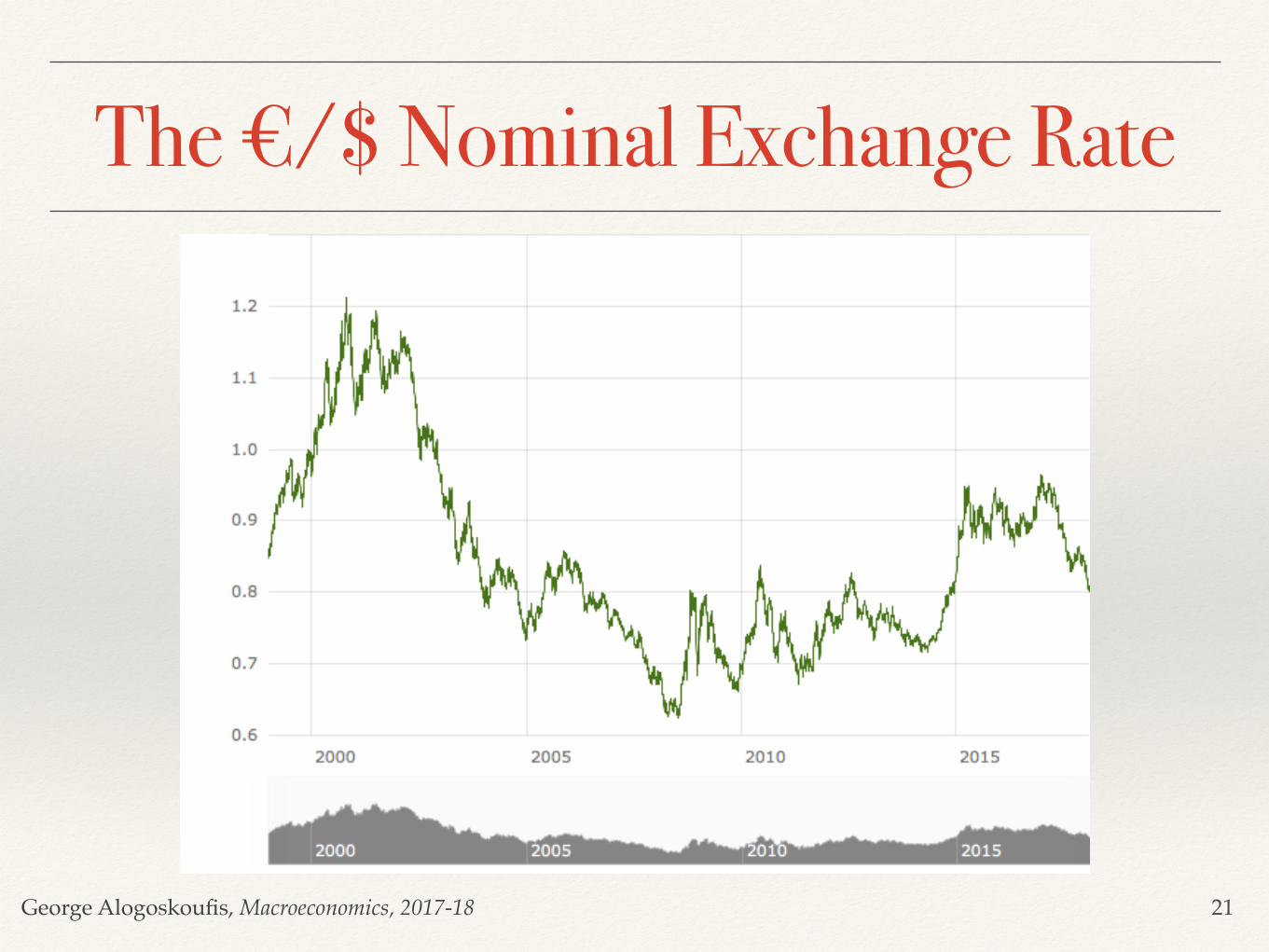
Suppose the domestic currency is the dollar and the foreign currency is the euro. S = 0.80 €/$ means that it takes 0.80 euros (€) for the purchase of one US dollar ($). If the rate changed to 0.85 then we say that the dollar has appreciated against the euro (or that the euro has depreciated against the dollar).

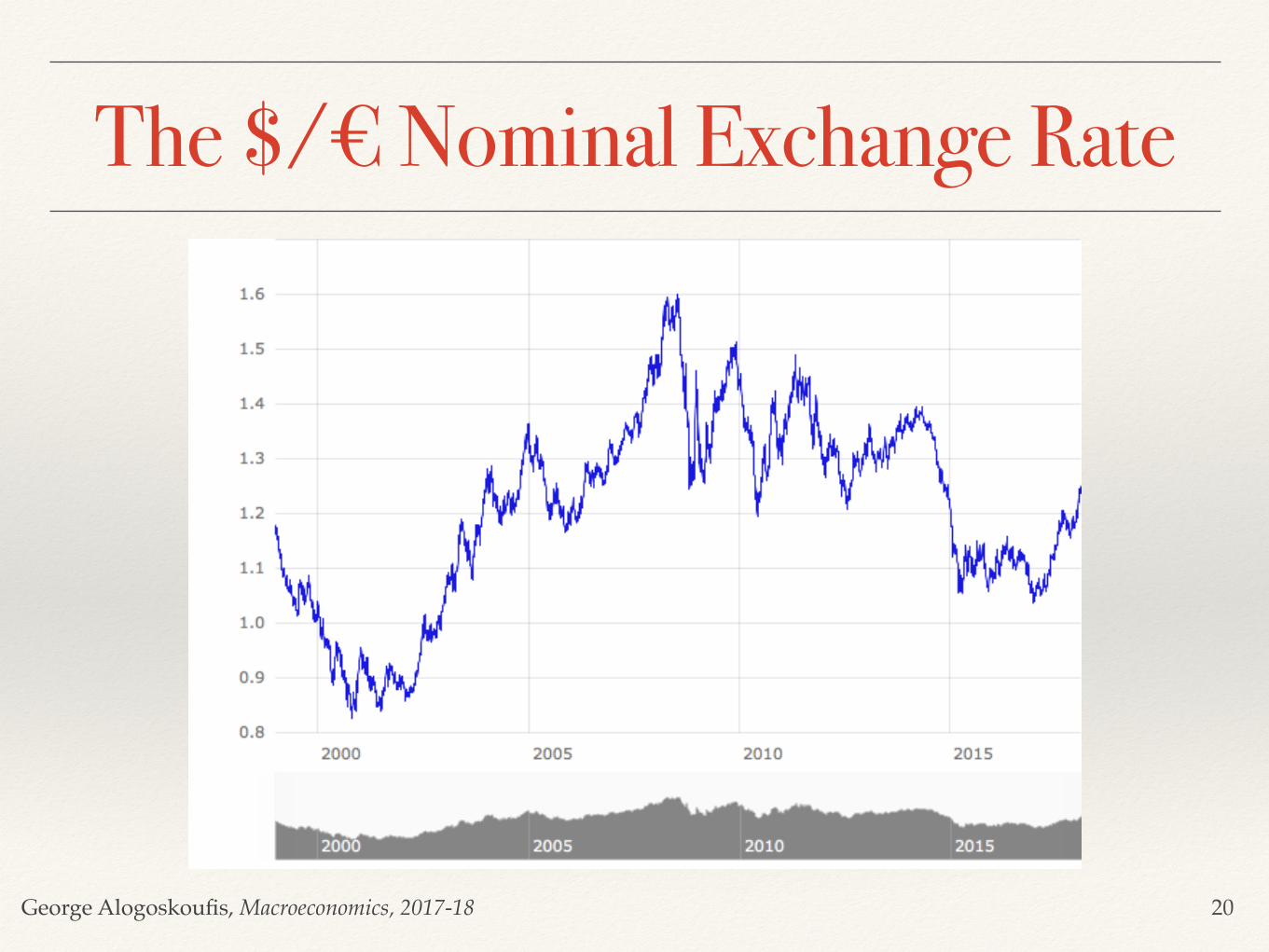
Suppose the domestic currency is the euro and the foreign currency is the dollar. This would be relevant for an analysis focused on the Euro area. S = 1.25 $/€ means that it takes 1.25 US dollars ($) for the purchase of one euro (€). If the rate changed to 1.30 then we say that the euro has appreciated against the dollar (or that the dollar has depreciated against the euro).

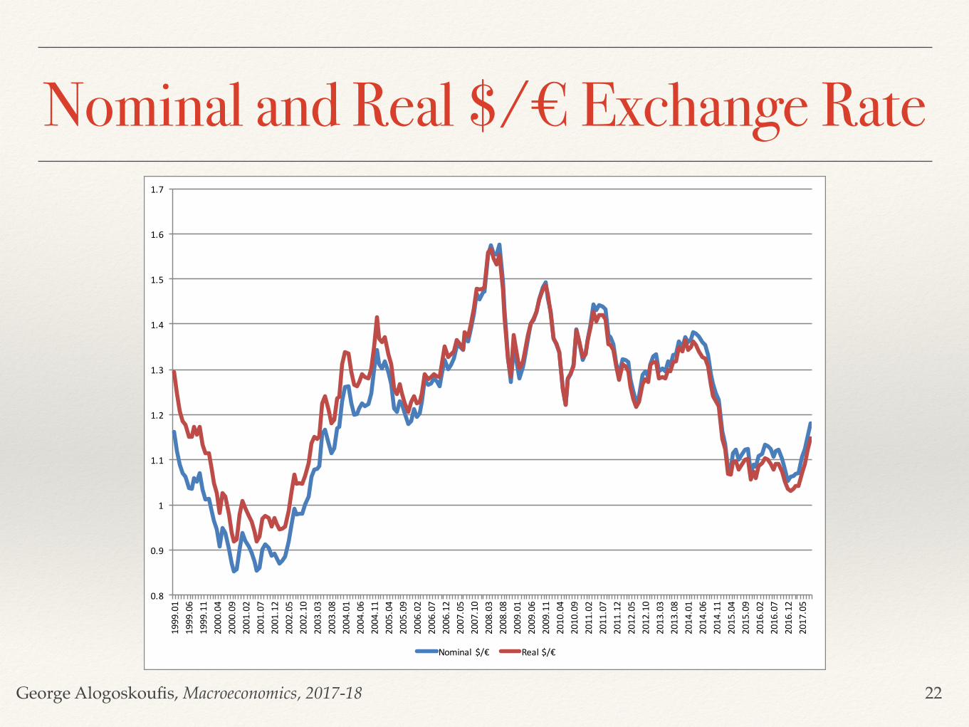
The bilateral real exchange rate (Q) is defined as the ratio of the two countries' price levels expressed in a common currency. We shall define it as,

Q=S (P/P*)

where P is the domestic price level in domestic currency, and P* is the foreign price level, in foreign currency.

If our focus is the US, S is defined as €/$, P is the domestic price level in dollars, and P* is the foreign price level in euros. A rise in Q means that the dollar has appreciated in real terms against the euro, in the sense that US prices in terms of euros have risen relative to European prices, or that US prices have risen relative to European prices expressed in dollars. A fall in Q means that the dollar has depreciated in real terms against the euro, in the sense that US prices in terms of euros have fallen relative to European prices, or that US prices have fallen relative to European prices expressed in dollars.

19


The $/€ Nominal Exchange Rate

20


The €/$ Nominal Exchange Rate

21


Nominal and Real $/€ Exchange Rate

22

0.8

0.9

1

1.1

1.2

1.3

1.4

1.5

1.6

1.71999.01

1999.06

1999.11

2000.04

2000.09

2001.02

2001.07

2001.12

2002.05

2002.10

2003.03

2003.08

2004.01

2004.06

2004.11

2005.04

2005.09

2006.02

2006.07

2006.12

2007.05

2007.10

2008.03

2008.08

2009.01

2009.06

2009.11

2010.04

2010.09

2011.02

2011.07

2011.12

2012.05

2012.10

2013.03

2013.08

2014.01

2014.06

2014.11

2015.04

2015.09

2016.02

2016.07

2016.12

2017.05

Nominal $/€ Real$/€


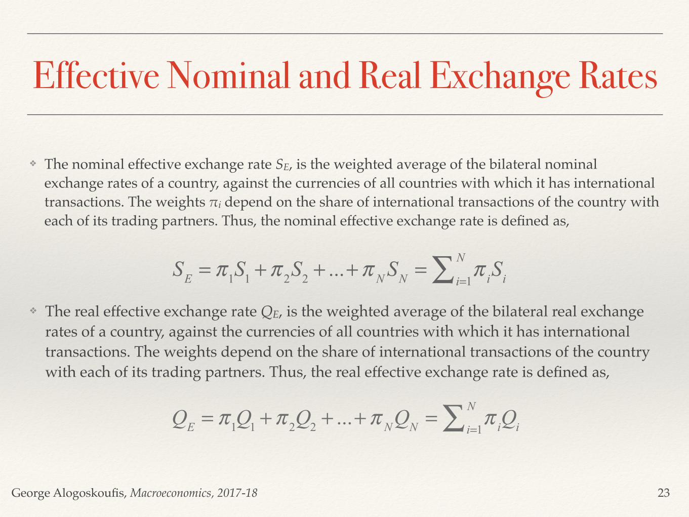
Effective Nominal and Real Exchange Rates

❖ The nominal effective exchange rate SE, is the weighted average of the bilateral nominal exchange rates of a country, against the currencies of all countries with which it has international transactions. The weights πi depend on the share of international transactions of the country with each of its trading partners. Thus, the nominal effective exchange rate is defined as,

23

SE = π1S1 +π 2S2 + ...+π NSN = π ii=1

N∑ Si❖ The real effective exchange rate QE, is the weighted average of the bilateral real exchange

rates of a country, against the currencies of all countries with which it has international transactions. The weights depend on the share of international transactions of the country with each of its trading partners. Thus, the real effective exchange rate is defined as,

QE = π1Q1 +π 2Q2 + ...+π NQN = π ii=1

N∑ Qi


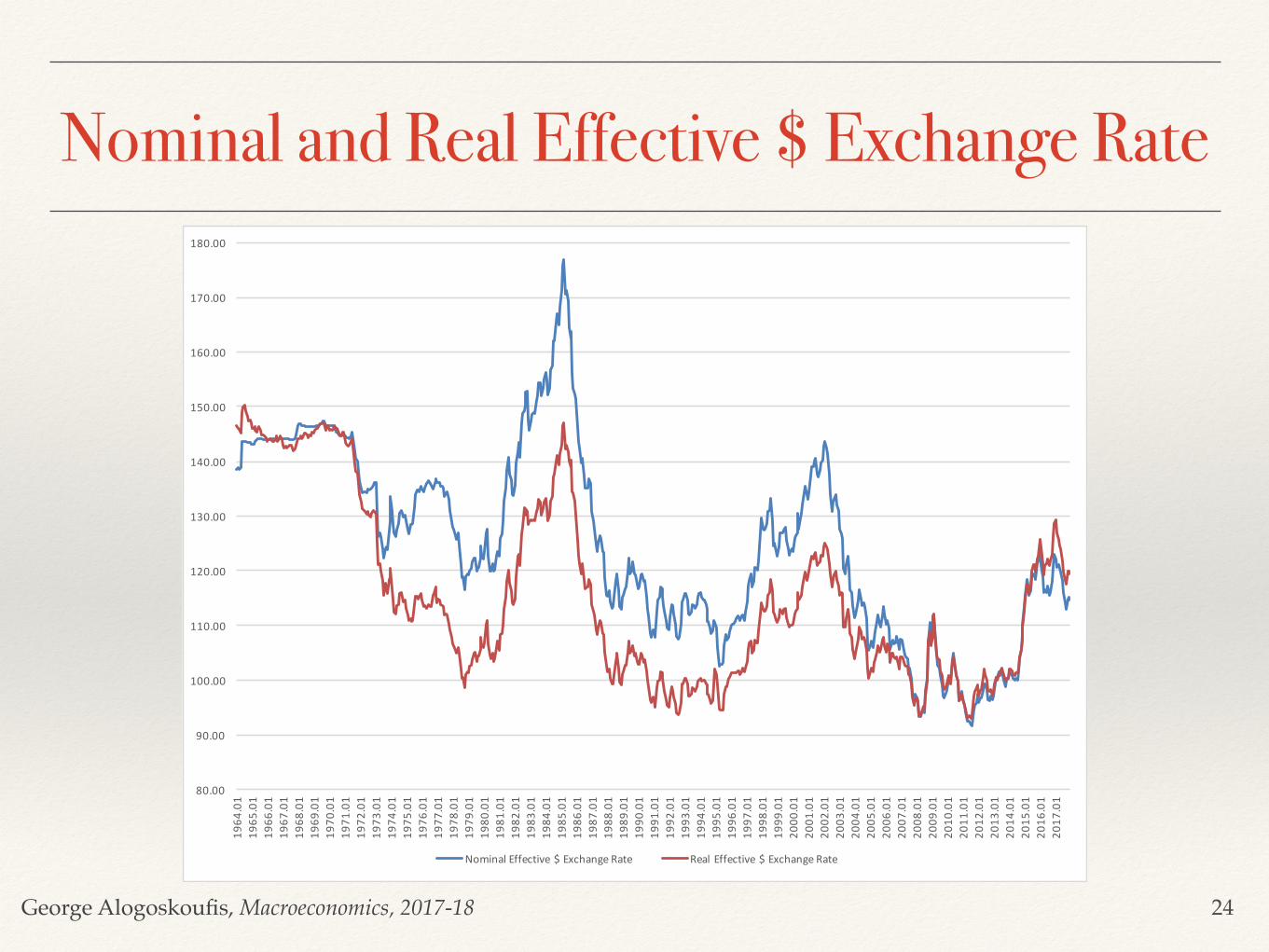
Nominal and Real Effective $ Exchange Rate

24

80.00

90.00

100.00

110.00

120.00

130.00

140.00

150.00

160.00

170.00

180.0019

64.01

1965

.01

1966

.01

1967

.01

1968

.01

1969

.01

1970

.01

1971

.01

1972

.01

1973

.01

1974

.01

1975

.01

1976

.01

1977

.01

1978

.01

1979

.01

1980

.01

1981

.01

1982

.01

1983

.01

1984

.01

1985

.01

1986

.01

1987

.01

1988

.01

1989

.01

1990

.01

1991

.01

1992

.01

1993

.01

1994

.01

1995

.01

1996

.01

1997

.01

1998

.01

1999

.01

2000

.01

2001

.01

2002

.01

2003

.01

2004

.01

2005

.01

2006

.01

2007

.01

2008

.01

2009

.01

2010

.01

2011

.01

2012

.01

2013

.01

2014

.01

2015

.01

2016

.01

2017

.01

NominalEffective$ExchangeRate RealEffective$ExchangeRate


The International Monetary System❖ The international monetary systems is the set of internationally agreed rules,

conventions and supporting institutions, that facilitate international trade, cross border investment and generally the reallocation of capital between nation states.

❖ It provides for means of payments acceptable between buyers and sellers of different nationality, including means of deferred payments (debt instruments).

❖ To operate successfully, it must inspire confidence, provide sufficient liquidity for fluctuating levels of trade and provide means and rules by which global imbalances can be corrected.

❖ The international monetary system can develop organically, as the collective result of numerous individual agreements between international economic factors spread over several decades, or it can arise from a single architectural vision, as happened with the post World War II system agreed at Bretton Woods in 1944.

25


Characteristics of International Monetary Systems

❖ The degree to which international trade in goods, services and capital is free.

❖ The means through which international transactions are settled and the internationally accepted means of payments.

❖ Whether exchange rates are fixed or flexible.

❖ The degree of symmetry or asymmetry in the benefits and obligations of different countries.

❖ Whether it is based in precious metals or not.

❖ These are some of the most critical characteristics concerning an international monetary system which have important implications for the the financing and correction of external imbalances.

26


Monetary Policy, Exchange Rates and Capital Mobility in Open Economies: The Trilemma of Open Economies

❖ The ability of the central bank of a country to pursue an independent monetary policy differs depending on the exchange rate regime and the regime of capital mobility.

❖ When there is free mobility of capital, the central bank has two basic options. It can either let the exchange rate fluctuate freely (floating exchange rates) without interventions in the foreign exchange market, or it can make interventions in the foreign exchange market (fixed or managed exchange rates). In the latter case, it transpires that it cannot pursue an independent monetary policy.

❖ To enable a central bank to pursue an independent monetary policy under a fixed or managed exchange rate regime, a country must impose restrictions on capital movements (capital controls).

❖ Of the three options of: 1. Fixed (or Managed) Exchange Rates, 2. An Independent National Monetary Policy and 3. Free Mobility of Capital, only two are available in a country. All three options are simultaneously incompatible.

❖ This is called the trilemma of open economies.

27


Fixed, Managed and Flexible Exchange Rates

❖ For about forty years before World War I (1879-1914) the main economies operated under an international monetary system called the international gold standard. This was a system of fixed exchange rates, based on gold, and the dominant international reserve currency of the time, the pound sterling.

❖ The interwar period was characterized by a variety of exchange rate regimes ranging from floating exchange rates in the first part of the 1920s, to a brief restoration of the international gold standard (1926-1931), to managed exchange rates and capital controls in the 1930s. This period is considered as one of international monetary instability, and is also marked by protectionism in international trade and the onset of the Great Depression.

❖ Between the end of World War II and 1973 the industrial countries operated a system of fixed but adjustable exchange rates, the Bretton Woods system, based on the US dollar (and partly gold), which was also underpinned by capital controls.

❖ From 1973 until today, the US, the Euro Area, Japan, the United Kingdom and Switzerland have chosen free capital mobility, and domestic monetary autonomy, resulting in a system of floating exchange rates. Other countries have chosen a variety of exchange rate regimes, ranging from floating to unilaterally fixed exchange rates.

28


Exchange Rate Regimes in the Post War Period

Between the end of World War II and 1973 the industrial economies operated a system of fixed exchange rates, the Bretton Woods system. In fixed exchange rate systems, the required level of cooperation between central banks and governments of the major economies is high, as it requires coordination of monetary, and budgetary policies in order to maintain and operate the system. Capital controls were gradually relaxed during the 1960s, but the system came under severe pressure towards the end of the decade.

From 1973 until today, the US, the Euro Area, Japan, the United Kingdom and Switzerland have chosen free capital mobility, and domestic monetary autonomy, resulting in a system of floating exchange rates. International monetary cooperation is much looser than in the Bretton Woods system.

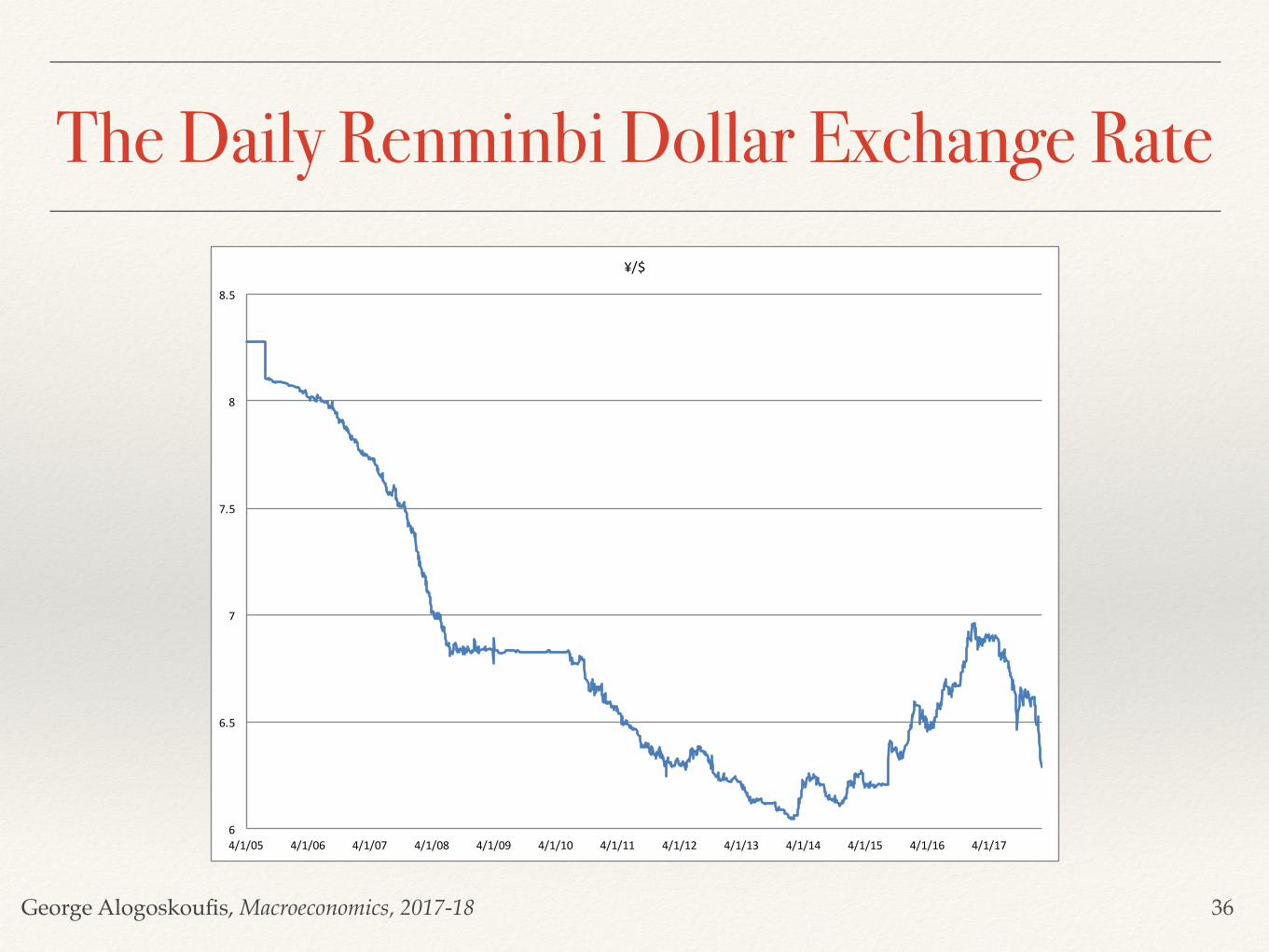
China has chosen capital controls in order to combine managed exchange rates with domestic monetary autonomy.

In 1978, the countries of the European Economic Community (later the European Union) established the European Monetary System, a system of fixed but adjustable exchange rates among their currencies. This later developed into a single currency, the euro, which materialized in 1999. The euro can be seen as an extreme form of fixed exchange rates under free capital mobility. As a result they economies of the Euro Area have given up their monetary autonomy, which has been delegated to the European Central Bank (ECB).

29


International Reserve Currencies❖ Unlike in national states, in international economic transactions there is no single government that can impose

the use of a single currency.

❖ Thus, the global economy ends up with a plurality of currencies, although usually only a few of them are fully acceptable internationally. Thus, only a few currencies are used as international units of account, international means of payment and international stores of value.

❖ Some currencies tend to become dominant, and are called international reserve currencies. Such currencies were sterling in the period of the international gold standard (1880-1914) and the dollar since the end of the First World War.

❖ International reserve currencies typically are issued by large or extremely open economies, with a large share in international trade and international portfolios of assets. The US dollar remains the dominant international currency for about a century. It is the major unit of pricing international imports and exports, and is widely used in foreign exchange transactions in international financial markets and as a reserve currency for other central banks.

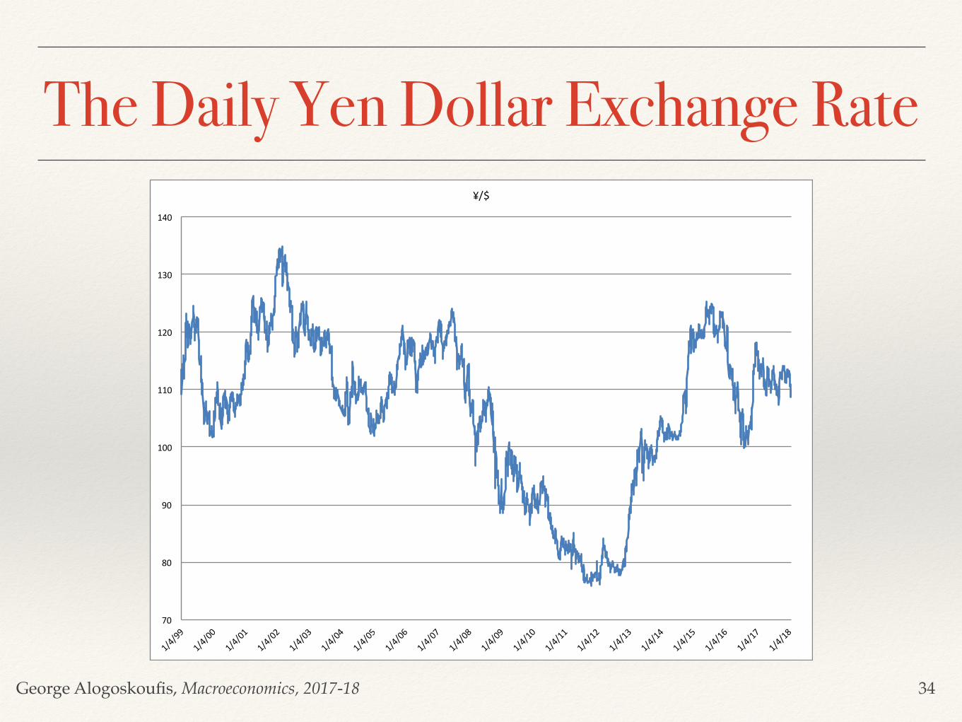
❖ The international monetary system today is basically tripolar, with a dominant role for the US dollar ($). The other two major currencies are the Euro (€) and the Japanese Yen (¥).

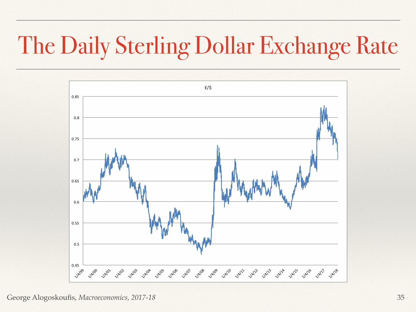
❖ In addition, the pound sterling (£), the Swiss franc and the Chinese renmimbi, or yuan, are significant international currencies.

30


Currency Convertibility❖ Convertibility is the quality that allows money or other financial instruments to be converted

into other liquid stores of value. Currency convertibility is an important factor in international exchanges, where instruments valued in different currencies must be exchanged.

❖ Historically, currency convertibility was defined in relation to precious metals, such as silver and gold.

❖ After World War I, convertibility of a currency is defined relative to the dominant international reserve currency, i.e. the dollar, and not necessarily in relation to gold.

❖ If the international reserve currency is convertible into a precious metal such as gold, the international monetary system is considered to be based on metallic standard.

❖ The international monetary system was loosely based on a metallic standard until 1968. In that year the US abolished the convertibility of the dollar into gold at a fixed price of $35 per ounce, resulting in the international monetary system getting completely delinked from gold.

31


Dollar Sterling Nominal Exchange Rate, 1791-2016

32

0.00

2.00

4.00

6.00

8.00

10.00

12.001791

1796

1801

1806

1811

1816

1821

1826

1831

1836

1841

1846

1851

1856

1861

1866

1871

1876

1881

1886

1891

1896

1901

1906

1911

1916

1921

1926

1931

1936

1941

1946

1951

1956

1961

1966

1971

1976

1981

1986

1991

1996

2001

2006

2011

2016

$/£ExchangeRate


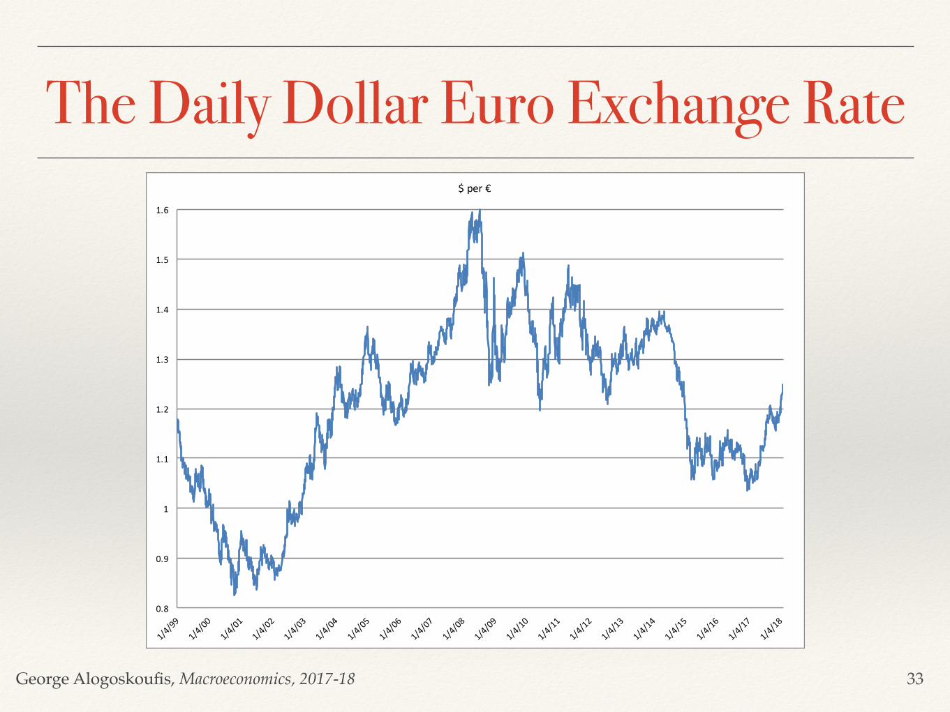
The Daily Dollar Euro Exchange Rate

33

0.8

0.9

1

1.1

1.2

1.3

1.4

1.5

1.6

$per€


The Daily Yen Dollar Exchange Rate

34

70

80

90

100

110

120

130

140

¥/$


The Daily Sterling Dollar Exchange Rate

35

0.45

0.5

0.55

0.6

0.65

0.7

0.75

0.8

0.85

£/$


The Daily Renminbi Dollar Exchange Rate

36

6

6.5

7

7.5

8

8.5

4/1/05 4/1/06 4/1/07 4/1/08 4/1/09 4/1/10 4/1/11 4/1/12 4/1/13 4/1/14 4/1/15 4/1/16 4/1/17

¥/$


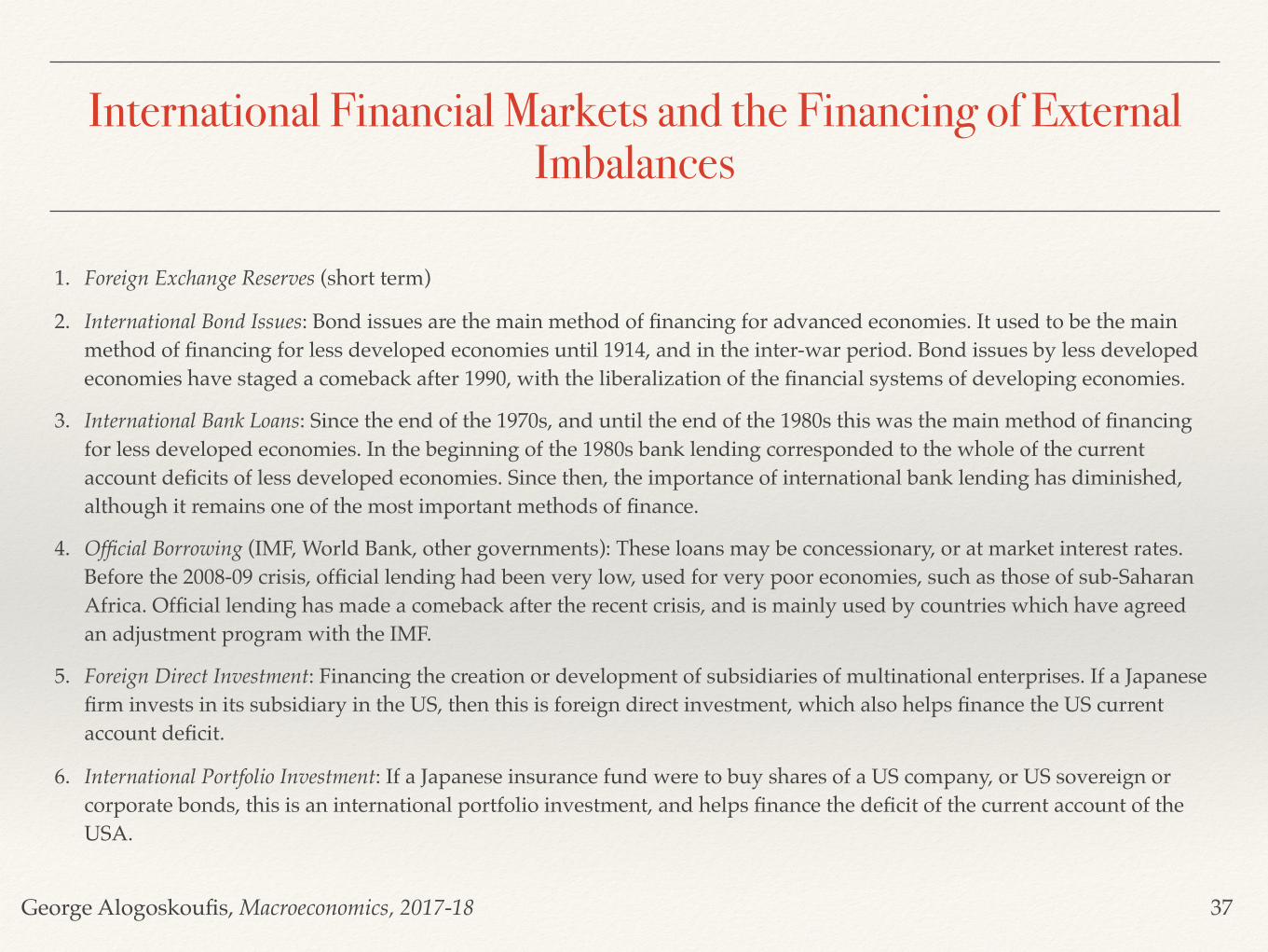
International Financial Markets and the Financing of External Imbalances

1. Foreign Exchange Reserves (short term)

2. International Bond Issues: Bond issues are the main method of financing for advanced economies. It used to be the main method of financing for less developed economies until 1914, and in the inter-war period. Bond issues by less developed economies have staged a comeback after 1990, with the liberalization of the financial systems of developing economies.

3. International Bank Loans: Since the end of the 1970s, and until the end of the 1980s this was the main method of financing for less developed economies. In the beginning of the 1980s bank lending corresponded to the whole of the current account deficits of less developed economies. Since then, the importance of international bank lending has diminished, although it remains one of the most important methods of finance.

4. Official Borrowing (IMF, World Bank, other governments): These loans may be concessionary, or at market interest rates. Before the 2008-09 crisis, official lending had been very low, used for very poor economies, such as those of sub-Saharan Africa. Official lending has made a comeback after the recent crisis, and is mainly used by countries which have agreed an adjustment program with the IMF.

5. Foreign Direct Investment: Financing the creation or development of subsidiaries of multinational enterprises. If a Japanese firm invests in its subsidiary in the US, then this is foreign direct investment, which also helps finance the US current account deficit.

6. International Portfolio Investment: If a Japanese insurance fund were to buy shares of a US company, or US sovereign or corporate bonds, this is an international portfolio investment, and helps finance the deficit of the current account of the USA.

37


Finance through Debt and non Debt Securities

❖ International bonds, international bank loans and official lending constitute debt, whereas foreign direct investment and international portfolio investment in shares does not constitute debt.

❖ The difference between the two methods of financing is that in debt contracts, the borrower agrees to repay in specific installments (interest and amortization) to the lender, irrespective of conditions, while in the case of equity investment, the investor shares in the profits of firms only if the firms make profits.

38


Differences between Advanced and Less Developed Economies

❖ The problem with less developed economies is that a large part of the financing of their current account deficits is through external debt, and in particular debt denominated in foreign currencies. International investors tend to refrain from assuming the currency risk associated with a peripheral currency, even if they assume the country risk.

❖ On the other hand, the major advanced economies, whose currencies are widely traded internationally, almost always borrow in their own currency. Thus, the US borrows in US dollars, the Euro Zone economies in euro’s, Japan in Japanese yen, Britain in sterling. Even Switzerland, due to the international acceptance of the Swiss franc, borrows in its own currency.

❖ A country that can borrow in its own currency has significant advantages over countries which cannot do this. It can continue servicing its loans, even if it has to resort to issuing money in order to pay its creditors. So it does not run the risk of default. This option is not available to developing economies which borrow in foreign currency.

39


The “Original Sin” of Less Developed Economies and the “Exorbitant Privilege” of the USA

❖ The inability of less developed economies to borrow in their own currency, is often called the original sin. On the other hand, the ability of the US to borrow in dollars, and in this way to reduce the real value of its international obligations, is often referred to as the exorbitant privilege of the US.

❖ It is also worth noting that, as shown by the recent crisis in the peripheral economies of the Euro Zone, participation in a single currency area like the euro area does not ultimately absolve a less developed economy from the original sin.

❖ The governments of a small open economies participating in the Euro Zone cannot rely on the European Central Bank (ECB) to lend them euros to service their euro denominated debts, or the debts of their banks. This is because of the ECB's political independence and the prohibition of monetary financing of budget deficits in the Euro Zone. In essence, the statutes of the ECB do not allow it to function effectively as a lender of last resort to Euro Zone governments, in contrast to the central banks in the US, Britain or Japan who do in fact act as lenders of last resort.

40

5. openness in goods and financial markets: the current ... · openness in goods and financial...

Documents