5 Random Walks and Markov Chains

A random walk on a directed graph consists of a sequence of vertices generated froma start vertex by selecting an edge, traversing the edge to a new vertex, and repeatingthe process. We will see that if the graph is strongly connected, then the fraction of timethe walk spends at the various vertices of the graph converges to a stationary probabilitydistribution.

Since the graph is directed, there might be vertices with no out edges and hencenowhere for the walk to go. Vertices in a strongly connected component with no in edgesfrom the remainder of the graph can never be reached unless the component contains thestart vertex. Once a walk leaves a strongly connected component it can never return.Most of our discussion of random walks will involve strongly connected graphs.

Start a random walk at a vertex x0 and think of the starting probability distributionas putting a mass of one on x0 and zero on every other vertex. More generally, onecould start with any probability distribution p, where p is a row vector with nonnegativecomponents summing to one, with px being the probability of starting at vertex x. Theprobability of being at vertex x at time t + 1 is the sum over each adjacent vertex y ofbeing at y at time t and taking the transition from y to x. Let p(t) be a row vector witha component for each vertex specifying the probability mass of the vertex at time t andlet p(t+1) be the row vector of probabilities at time t+ 1. In matrix notation4

p(t)P = p(t+1)

where the ijth entry of the matrix P is the probability of the walk at vertex i selectingthe edge to vertex j.

A fundamental property of a random walk is that in the limit, the long-term averageprobability of being at a particular vertex is independent of the start vertex, or an initialprobability distribution over vertices, provided only that the underlying graph is stronglyconnected. The limiting probabilities are called the stationary probabilities. This funda-mental theorem is proved in the next section.

A special case of random walks, namely random walks on undirected graphs, hasimportant connections to electrical networks. Here, each edge has a parameter calledconductance, like the electrical conductance, and if the walk is at vertex u, it choosesthe edge from among all edges incident to u to walk to the next vertex with probabilitiesproportional to their conductance. Certain basic quantities associated with random walksare hitting time, the expected time to reach vertex y starting at vertex x, and cover time,the expected time to visit every vertex. Qualitatively, these quantities are all boundedabove by polynomials in the number of vertices. The proofs of these facts will rely on the

4Probability vectors are represented by row vectors to simplify notation in equations like the one here.

186

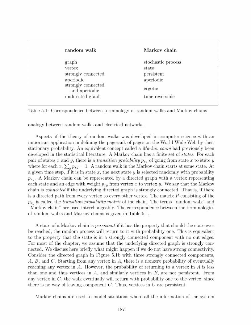
random walk Markov chain

graph stochastic processvertex statestrongly connected persistentaperiodic aperiodicstrongly connected

and aperiodic ergotic

undirected graph time reversible

Table 5.1: Correspondence between terminology of random walks and Markov chains

analogy between random walks and electrical networks.

Aspects of the theory of random walks was developed in computer science with animportant application in defining the pagerank of pages on the World Wide Web by theirstationary probability. An equivalent concept called a Markov chain had previously beendeveloped in the statistical literature. A Markov chain has a finite set of states. For eachpair of states x and y, there is a transition probability pxy of going from state x to state ywhere for each x,

∑

y pxy = 1. A random walk in the Markov chain starts at some state. Ata given time step, if it is in state x, the next state y is selected randomly with probabilitypxy. A Markov chain can be represented by a directed graph with a vertex representingeach state and an edge with weight pxy from vertex x to vertex y. We say that the Markovchain is connected if the underlying directed graph is strongly connected. That is, if thereis a directed path from every vertex to every other vertex. The matrix P consisting of thepxy is called the transition probability matrix of the chain. The terms “random walk” and“Markov chain” are used interchangeably. The correspondence between the terminologiesof random walks and Markov chains is given in Table 5.1.

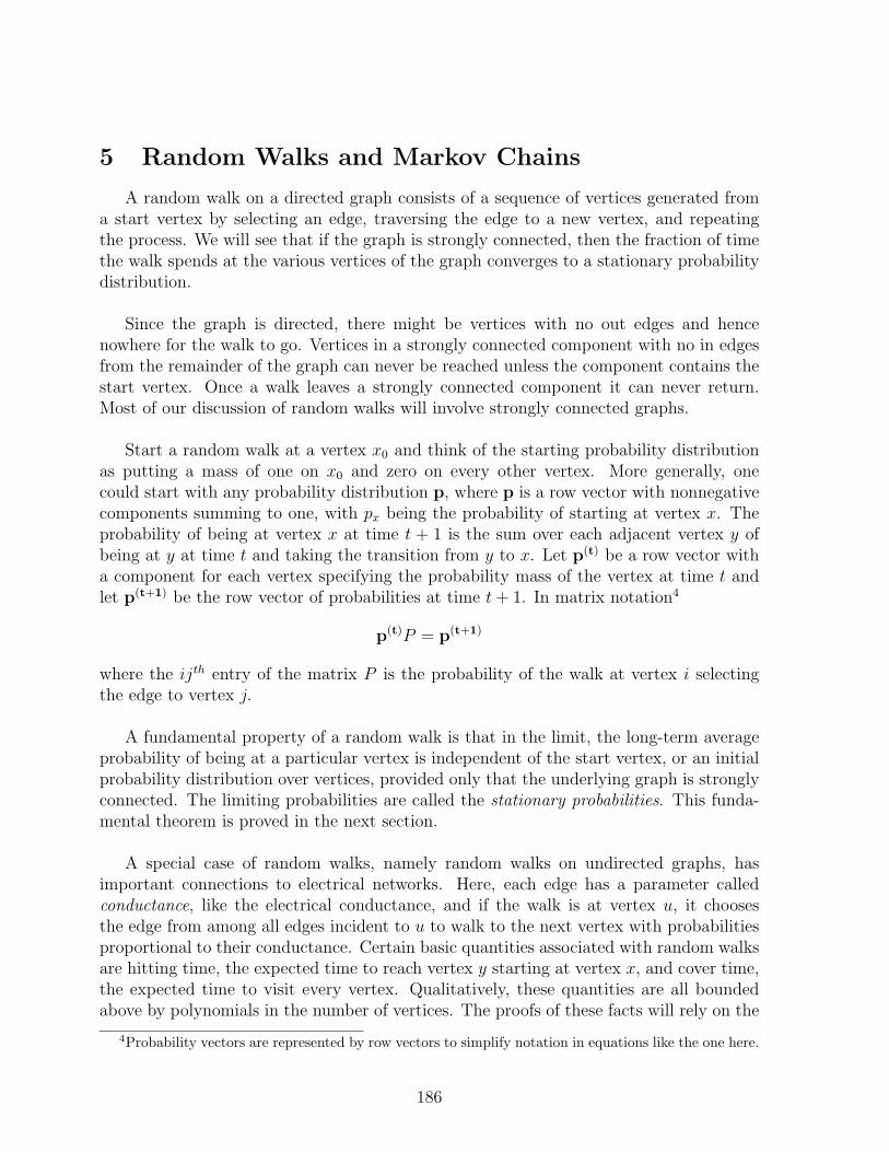
A state of a Markov chain is persistent if it has the property that should the state everbe reached, the random process will return to it with probability one. This is equivalentto the property that the state is in a strongly connected component with no out edges.For most of the chapter, we assume that the underlying directed graph is strongly con-nected. We discuss here briefly what might happen if we do not have strong connectivity.Consider the directed graph in Figure 5.1b with three strongly connected components,A, B, and C. Starting from any vertex in A, there is a nonzero probability of eventuallyreaching any vertex in A. However, the probability of returning to a vertex in A is lessthan one and thus vertices in A, and similarly vertices in B, are not persistent. Fromany vertex in C, the walk eventually will return with probability one to the vertex, sincethere is no way of leaving component C. Thus, vertices in C are persistent.

Markov chains are used to model situations where all the information of the system

187

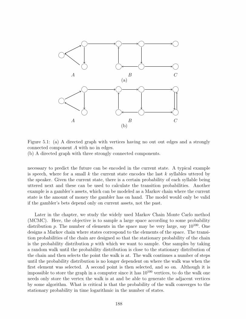
A B C(a)

A B C(b)

Figure 5.1: (a) A directed graph with vertices having no out out edges and a stronglyconnected component A with no in edges.(b) A directed graph with three strongly connected components.

necessary to predict the future can be encoded in the current state. A typical exampleis speech, where for a small k the current state encodes the last k syllables uttered bythe speaker. Given the current state, there is a certain probability of each syllable beinguttered next and these can be used to calculate the transition probabilities. Anotherexample is a gambler’s assets, which can be modeled as a Markov chain where the currentstate is the amount of money the gambler has on hand. The model would only be validif the gambler’s bets depend only on current assets, not the past.

Later in the chapter, we study the widely used Markov Chain Monte Carlo method(MCMC). Here, the objective is to sample a large space according to some probabilitydistribution p. The number of elements in the space may be very large, say 10100. Onedesigns a Markov chain where states correspond to the elements of the space. The transi-tion probabilities of the chain are designed so that the stationary probability of the chainis the probability distribution p with which we want to sample. One samples by takinga random walk until the probability distribution is close to the stationary distribution ofthe chain and then selects the point the walk is at. The walk continues a number of stepsuntil the probability distribution is no longer dependent on where the walk was when thefirst element was selected. A second point is then selected, and so on. Although it isimpossible to store the graph in a computer since it has 10100 vertices, to do the walk oneneeds only store the vertex the walk is at and be able to generate the adjacent verticesby some algorithm. What is critical is that the probability of the walk converges to thestationary probability in time logarithmic in the number of states.

188

We mention two motivating examples. The first is to estimate the probability of aregion R in d-space according to a probability density like the Gaussian. Put down agrid and make each grid point that is in R a state of the Markov chain. Given a proba-bility density p, design transition probabilities of a Markov chain so that the stationarydistribution is exactly p. In general, the number of states grows exponentially in the di-mension d, but the time to converge to the stationary distribution grows polynomially in d.

A second example is from physics. Consider an n×n grid in the plane with a particleat each grid point. Each particle has a spin of ±1. There are 2n

2

spin configurations.The energy of a configuration is a function of the spins. A central problem in statisticalmechanics is to sample a spin configuration according to their probability. It is easy todesign a Markov chain with one state per spin configuration so that the stationary prob-ability of a state is proportional to the state’s energy. If a random walk gets close to thestationary probability in time polynomial to n rather than 2n

2

, then one can sample spinconfigurations according to their probability.

A quantity called the mixing time, loosely defined as the time needed to get close tothe stationary distribution, is often much smaller than the number of states. In Section5.8, we relate the mixing time to a combinatorial notion called normalized conductanceand derive good upper bounds on the mixing time in many cases.

5.1 Stationary Distribution

Let p(t) be the probability distribution after t steps of a random walk. Define thelong-term probability distribution a(t) by

a(t) =1

t

(p(0) + p(1) + · · ·+ p(t−1)

).

The fundamental theorem of Markov chains asserts that the long-term probability distri-bution of a connected Markov chain converges to a unique limit probability vector, whichwe denote by π. Executing one more step, starting from this limit distribution, we getback the same distribution. In matrix notation, πP = π where P is the matrix of transi-tion probabilities. In fact, there is a unique probability vector (nonnegative componentssumming to one) satisfying πP = π and this vector is the limit. Also since one step doesnot change the distribution, any number of steps would not either. For this reason, π iscalled the stationary distribution.

Before proving the fundamental theorem of Markov chains, we first prove a technicallemma.

Lemma 5.1 Let P be the transition probability matrix for a connected Markov chain.The n× (n+1) matrix A = [P − I , 1] obtained by augmenting the matrix P − I with anadditional column of ones has rank n.

189

Proof: If the rank of A = [P − I,1] was less than n there would be two linearly indepen-dent solutions to Ax = 0. Each row in P sums to one so each row in P − I sums to zero.Thus x = (1, 0), where all but the last coordinate of x is 1, is one solution to Ax = 0.Assume there was a second solution (x, α) perpendicular to (1, 0). Then (P−I)x+α1 = 0or xi =

∑

j pijxj +α. Each xi is a convex combination of some xj plus α. Let S be the set

of i for which xi attains its maximum value. S is not empty since x is perpendicular to 1and hence

∑

j xj = 0. Connectedness implies that some xk of maximum value is adjacentto some xl of lower value. Thus, xk >

∑

j pkjxj. Therefore α must be greater than 0 inxk =

∑

j pkjxj + α..

A symmetric argument with T the set of i with xi taking its minimum value impliesα < 0 producing a contradiction thereby proving the lemma.

Theorem 5.2 (Fundamental Theorem of Markov Chains) For a connected Markovchain there is a unique probability vector π satisfying πP = π. Moreover, for any startingdistribution, lim

t→∞a(t) exists and equals π.

Proof: Note that a(t) is itself a probability vector, since its components are nonnegativeand sum to 1. Run one step of the Markov chain starting with distribution a(t); thedistribution after the step is a(t)P . Calculate the change in probabilities due to this step.

a(t)P − a(t) =1

t

[p(0)P + p(1)P + · · ·+ p(t−1)P

]− 1

t

[p(0) + p(1) + · · ·+ p(t−1)

]

=1

t

[p(1) + p(2) + · · ·+ p(t)

]− 1

t

[p(0) + p(1) + · · ·+ p(t−1)

]

=1

t

(p(t) − p(0)

).

Thus, b(t) = a(t)P − a(t) satisfies |b(t)| ≤ 2t→ 0, as t → ∞.

By Lemma 5.1 above, A has rank n. The n × n submatrix B of A consisting of allits columns except the first is invertible. Let c(t) be obtained from b(t) by removing thefirst entry. Then, a(t)B = [c(t), 1] and so a(t) = [c(t) , 1]B−1 → [0 , 1]B−1. We have thetheorem with π = [0 , 1]B−1.

Observe that the expected time rx for a Markov chain starting in state x to return tostate x is the reciprocal of the stationary probability of x. That is rx = 1

πx. Intuitively

this follows by observing that if a long walk always returns to state x in exactly rx steps,the frequency of being in a state x would be 1

rx. A rigorous proof requires the Strong Law

of Large Numbers.

We finish this section with the following lemma useful in establishing that a probabilitydistribution is the stationary probability distribution for a random walk on a connectedgraph with edge probabilities.

190

Lemma 5.3 For a random walk on a strongly connected graph with probabilities on theedges, if the vector π satisfies πxpxy = πypyx for all x and y and

∑

x πx = 1, then π isthe stationary distribution of the walk.

Proof: Since π satisfies πxpxy = πypyx, take the sum of both sides to get πx =∑

y

πypyx

and hence π satisfies π = πP. By Theorem 5.2, π is the unique stationary probability.

5.2 Electrical Networks and Random Walks

In the next few sections, we study the relationship between electrical networks andrandom walks on undirected graphs. The graphs have nonnegative weights on each edge.A step is executed by picking a random edge from the current vertex with probabilityproportional to the edge’s weight and traversing the edge.

An electrical network is a connected, undirected graph in which each edge (x, y) hasa resistance rxy > 0. In what follows, it is easier to deal with conductance defined as thereciprocal of resistance, cxy = 1

rxy, rather than resistance. Associated with an electrical

network is a random walk on the underlying graph defined by assigning a probabilitypxy = cxy

cxto the edge (x, y) incident to the vertex x, where the normalizing constant cx

equals∑

y

cxy. Note that although cxy equals cyx, the probabilities pxy and pyx may not be

equal due to the normalization required to make the probabilities at each vertex sum toone. We shall soon see that there is a relationship between current flowing in an electricalnetwork and a random walk on the underlying graph.

Since we assume that the undirected graph is connected, by Theorem 5.2 there isa unique stationary probability distribution.The stationary probability distribution is πwhere πx = cx

c0where c0 =

∑

x

cx. To see this, for all x and y

πxpxy =cxc0

cxycx

=cxyc0

=cyc0

cyxcy

= πypyx

and hence by Lemma 5.3, π is the unique stationary probability.

Harmonic functions

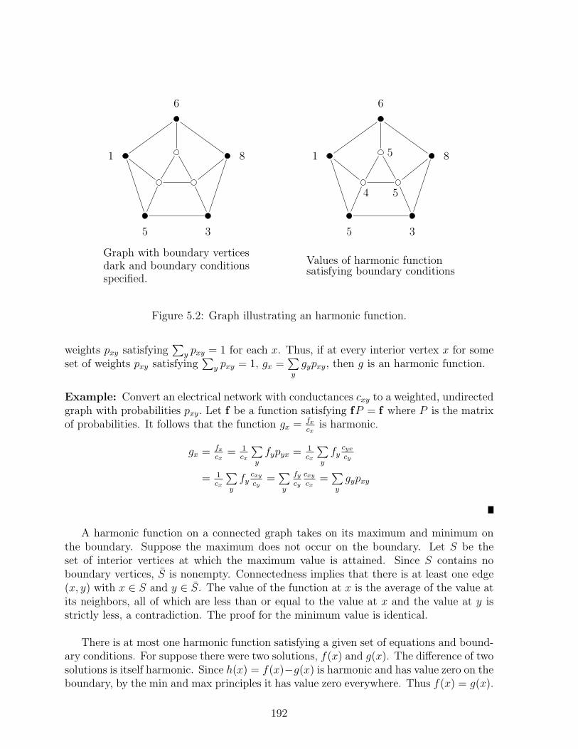
Harmonic functions are useful in developing the relationship between electrical net-works and random walks on undirected graphs. Given an undirected graph, designatea nonempty set of vertices as boundary vertices and the remaining vertices as interiorvertices. A harmonic function g on the vertices is one in which the value of the functionat the boundary vertices is fixed to some boundary condition and the value of g at anyinterior vertex x is a weighted average of the values at all the adjacent vertices y, with

191

6

8

35

1

Graph with boundary verticesdark and boundary conditionsspecified.

6

8

35

1 5

54

Values of harmonic functionsatisfying boundary conditions

Figure 5.2: Graph illustrating an harmonic function.

weights pxy satisfying∑

y pxy = 1 for each x. Thus, if at every interior vertex x for someset of weights pxy satisfying

∑

y pxy = 1, gx =∑

y

gypxy, then g is an harmonic function.

Example: Convert an electrical network with conductances cxy to a weighted, undirectedgraph with probabilities pxy. Let f be a function satisfying fP = f where P is the matrixof probabilities. It follows that the function gx = fx

cxis harmonic.

gx = fxcx

= 1cx

∑

y

fypyx = 1cx

∑

y

fycyxcy

= 1cx

∑

y

fycxycy

=∑

y

fycy

cxycx

=∑

y

gypxy

A harmonic function on a connected graph takes on its maximum and minimum onthe boundary. Suppose the maximum does not occur on the boundary. Let S be theset of interior vertices at which the maximum value is attained. Since S contains noboundary vertices, S is nonempty. Connectedness implies that there is at least one edge(x, y) with x ∈ S and y ∈ S. The value of the function at x is the average of the value atits neighbors, all of which are less than or equal to the value at x and the value at y isstrictly less, a contradiction. The proof for the minimum value is identical.

There is at most one harmonic function satisfying a given set of equations and bound-ary conditions. For suppose there were two solutions, f(x) and g(x). The difference of twosolutions is itself harmonic. Since h(x) = f(x)−g(x) is harmonic and has value zero on theboundary, by the min and max principles it has value zero everywhere. Thus f(x) = g(x).

192

The analogy between electrical networks and random walks

There are important connections between electrical networks and random walks onundirected graphs. Choose two vertices a and b. For reference purposes let the voltagevb equal zero. Attach a current source between a and b so that the voltage va equalsone. Fixing the voltages at va and vb induces voltages at all other vertices along with acurrent flow through the edges of the network. The analogy between electrical networksand random walks is the following. Having fixed the voltages at the vertices a and b, thevoltage at an arbitrary vertex x equals the probability of a random walk starting at xreaching a before reaching b. If the voltage va is adjusted so that the current flowing intovertex a corresponds to one walk, then the current flowing through an edge is the netfrequency with which a random walk from a to b traverses the edge.

Probabilistic interpretation of voltages

Before showing that the voltage at an arbitrary vertex x equals the probability of arandom walk starting at x reaching a before reaching b, we first show that the voltagesform a harmonic function. Let x and y be adjacent vertices and let ixy be the currentflowing through the edge from x to y. By Ohm’s law,

ixy =vx − vyrxy

= (vx − vy)cxy.

By Kirchhoff’s law the currents flowing out of each vertex sum to zero.

∑

y

ixy = 0

Replacing currents in the above sum by the voltage difference times the conductanceyields

∑

y

(vx − vy)cxy = 0

orvx∑

y

cxy =∑

y

vycxy.

Observing that∑

y

cxy = cx and that pxy = cxycx, yields vxcx =

∑

y

vypxycx. Hence,

vx =∑

y

vypxy. Thus, the voltage at each vertex x is a weighted average of the volt-

ages at the adjacent vertices. Hence the voltages form a harmonic function with a, b asthe boundary.

Let px be the probability that a random walk starting at vertex x reaches a before b.Clearly pa = 1 and pb = 0. Since va = 1 and vb = 0, it follows that pa = va and pb = vb.

193

Furthermore, the probability of the walk reaching a from x before reaching b is the sumover all y adjacent to x of the probability of the walk going from x to y in the first stepand then reaching a from y before reaching b. That is

px =∑

y

pxypy.

Hence, px is the same harmonic function as the voltage function vx and v and p satisfy thesame boundary conditions at a and b.. Thus, they are identical functions. The probabilityof a walk starting at x reaching a before reaching b is the voltage vx.

Probabilistic interpretation of current

In a moment, we will set the current into the network at a to have a value which we willequate with one random walk. We will then show that the current ixy is the net frequencywith which a random walk from a to b goes through the edge xy before reaching b. Letux be the expected number of visits to vertex x on a walk from a to b before reaching b.Clearly ub = 0. Every time the walk visits x, x not equal to a, it must come to x fromsome vertex y. Thus, the number of visits to x before reaching b is the sum over all y ofthe number of visits uy to y before reaching b times the probability pyx of going from yto x. For x not equal to b or a

ux =∑

y 6=b

uypyx.

Since ub = 0 and cxpxy = cypyx

ux =∑

all y

uycxpxycy

and hence ux

cx=∑

y

uy

cypxy. It follows that ux

cxis harmonic with a and b as the boundary

where the boundary conditions are ub = 0 and ua equals some fixed value. Now, ub

cb= 0.

Setting the current into a to one, fixed the value of va. Adjust the current into a so thatva equals ua

ca. Now ux

cxand vx satisfy the same harmonic conditions and thus are the same

harmonic function. Let the current into a correspond to one walk. Note that if the walkstarts at a and ends at b, the expected value of the difference between the number of timesthe walk leaves a and enters a must be one. This implies that the amount of current intoa corresponds to one walk.

Next we need to show that the current ixy is the net frequency with which a randomwalk traverses edge xy.

ixy = (vx − vy)cxy =

(ux

cx− uy

cy

)

cxy = uxcxycx

− uycxycy

= uxpxy − uypyx

The quantity uxpxy is the expected number of times the edge xy is traversed from x to yand the quantity uypyx is the expected number of times the edge xy is traversed from y to

194

x. Thus, the current ixy is the expected net number of traversals of the edge xy from x to y.

Effective resistance and escape probability

Set va = 1 and vb = 0. Let ia be the current flowing into the network at vertex a andout at vertex b. Define the effective resistance reff between a and b to be reff = va

iaand

the effective conductance ceff to be ceff = 1reff

. Define the escape probability, pescape, to

be the probability that a random walk starting at a reaches b before returning to a. Wenow show that the escape probability is

ceffca

. For convenience, assume that a and b arenot adjacent. A slight modification of our argument suffices for the case when a and b areadjacent.

ia =∑

y

(va − vy)cay

Since va = 1,

ia =∑

y

cay − ca∑

y

vycayca

= ca

[

1−∑

y

payvy

]

.

For each y adjacent to the vertex a, pay is the probability of the walk going from vertexa to vertex y. Earlier we showed that vy is the probability of a walk starting at y goingto a before reaching b. Thus,

∑

y

payvy is the probability of a walk starting at a returning

to a before reaching b and 1−∑

y

payvy is the probability of a walk starting at a reaching

b before returning to a. Thus, ia = capescape. Since va = 1 and ceff = iava, it follows that

ceff = ia . Thus, ceff = capescape and hence pescape =ceffca

.

For a finite connected graph the escape probability will always be nonzero. Nowconsider an infinite graph such as a lattice and a random walk starting at some vertexa. Form a series of finite graphs by merging all vertices at distance d or greater from ainto a single vertex b for larger and larger values of d. The limit of pescape as d goes toinfinity is the probability that the random walk will never return to a. If pescape → 0, theneventually any random walk will return to a. If pescape → q where q > 0, then a fractionof the walks never return. Thus, the escape probability terminology.

5.3 Random Walks on Undirected Graphs with Unit Edge Weights

We now focus our discussion on random walks on undirected graphs with uniformedge weights. At each vertex, the random walk is equally likely to take any edge. Thiscorresponds to an electrical network in which all edge resistances are one. Assume thegraph is connected. We consider questions such as what is the expected time for a random

195

walk starting at a vertex x to reach a target vertex y, what is the expected time until therandom walk returns to the vertex it started at, and what is the expected time to reachevery vertex?

Hitting time

The hitting time hxy, sometimes called discovery time, is the expected time of a ran-dom walk starting at vertex x to reach vertex y. Sometimes a more general definition isgiven where the hitting time is the expected time to reach a vertex y from a given startingprobability distribution.

One interesting fact is that adding edges to a graph may either increase or decreasehxy depending on the particular situation. Adding an edge can shorten the distance fromx to y thereby decreasing hxy or the edge could increase the probability of a random walkgoing to some far off portion of the graph thereby increasing hxy. Another interestingfact is that hitting time is not symmetric. The expected time to reach a vertex y from avertex x in an undirected graph may be radically different from the time to reach x from y.

We start with two technical lemmas. The first lemma states that the expected timeto traverse a path of n vertices is Θ (n2).

Lemma 5.4 The expected time for a random walk starting at one end of a path of nvertices to reach the other end is Θ(n2).

Proof: Consider walking from vertex 1 to vertex n in a graph consisting of a single pathof n vertices. Let hij, i < j, be the hitting time of reaching j starting from i. Now h12 = 1and

hi,i+1 =12+ 1

2(1 + hi−1,i+1) = 1 + 1

2(hi−1,i + hi,i+1) 2 ≤ i ≤ n− 1.

Solving for hi,i+1 yields the recurrence

hi,i+1 = 2 + hi−1,i.

Solving the recurrence yieldshi,i+1 = 2i− 1.

To get from 1 to n, go from 1 to 2, 2 to 3, etc. Thus

h1,n =n−1∑

i=1

hi,i+1 =n−1∑

i=1

(2i− 1)

= 2n−1∑

i=1

i−n−1∑

i=1

1

= 2n (n− 1)

2− (n− 1)

= (n− 1)2 .

196

The lemma says that in a random walk on a line where we are equally likely to takeone step to the right or left each time, the farthest we will go away from the start in nsteps is Θ(

√n).

The next lemma shows that the expected time spent at vertex i by a random walkfrom vertex 1 to vertex n in a chain of n vertices is 2(i− 1) for 2 ≤ i ≤ n− 1.

Lemma 5.5 Consider a random walk from vertex 1 to vertex n in a chain of n vertices.Let t(i) be the expected time spent at vertex i. Then

t (i) =

n− 1 i = 12 (n− i) 2 ≤ i ≤ n− 11 i = n.

Proof: Now t (n) = 1 since the walk stops when it reaches vertex n. Half of the time whenthe walk is at vertex n − 1 it goes to vertex n. Thus t (n− 1) = 2. For 3 ≤ i < n− 1,t (i) = 1

2[t (i− 1) + t (i+ 1)] and t (1) and t (2) satisfy t (1) = 1

2t (2) + 1 and t (2) =

t (1) + 12t (3). Solving for t(i+ 1) for 3 ≤ i < n− 1 yields

t(i+ 1) = 2t(i)− t(i− 1)

which has solution t(i) = 2(n− i) for 3 ≤ i < n− 1. Then solving for t(2) and t(1) yieldst (2) = 2 (n− 2) and t (1) = n− 1. Thus, the total time spent at vertices is

n− 1 + 2 (1 + 2 + · · ·+ n− 2) + 1 = (n− 1) + 2(n− 1)(n− 2)

2+ 1 = (n− 1)2 + 1

which is one more than h1n and thus is correct.

Adding edges to a graph might either increase or decrease the hitting time hxy. Con-sider the graph consisting of a single path of n vertices. Add edges to this graph to get thegraph in Figure 5.3 consisting of a clique of size n/2 connected to a path of n/2 vertices.Then add still more edges to get a clique of size n. Let x be the vertex at the midpoint ofthe original path and let y be the other endpoint of the path consisting of n/2 vertices asshown in the figure. In the first graph consisting of a single path of length n, hxy = Θ(n2).In the second graph consisting of a clique of size n/2 along with a path of length n/2,hxy = Θ(n3). To see this latter statement, note that starting at x, the walk will go downthe path towards y and return to x n/2 times on average before reaching y for the firsttime. Each time the walk in the path returns to x, with probability (n/2 − 1)/(n/2) itenters the clique and thus on average enters the clique Θ(n) times before starting downthe path again. Each time it enters the clique, it spends Θ(n) time in the clique beforereturning to x. Thus, each time the walk returns to x from the path it spends Θ(n2) timein the clique before starting down the path towards y for a total expected time that is

197

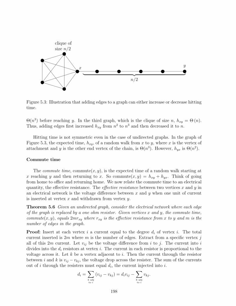
xy

n/2

︸ ︷︷ ︸

clique ofsize n/2

Figure 5.3: Illustration that adding edges to a graph can either increase or decrease hittingtime.

Θ(n3) before reaching y. In the third graph, which is the clique of size n, hxy = Θ(n).Thus, adding edges first increased hxy from n2 to n3 and then decreased it to n.

Hitting time is not symmetric even in the case of undirected graphs. In the graph ofFigure 5.3, the expected time, hxy, of a random walk from x to y, where x is the vertex ofattachment and y is the other end vertex of the chain, is Θ(n3). However, hyx is Θ(n2).

Commute time

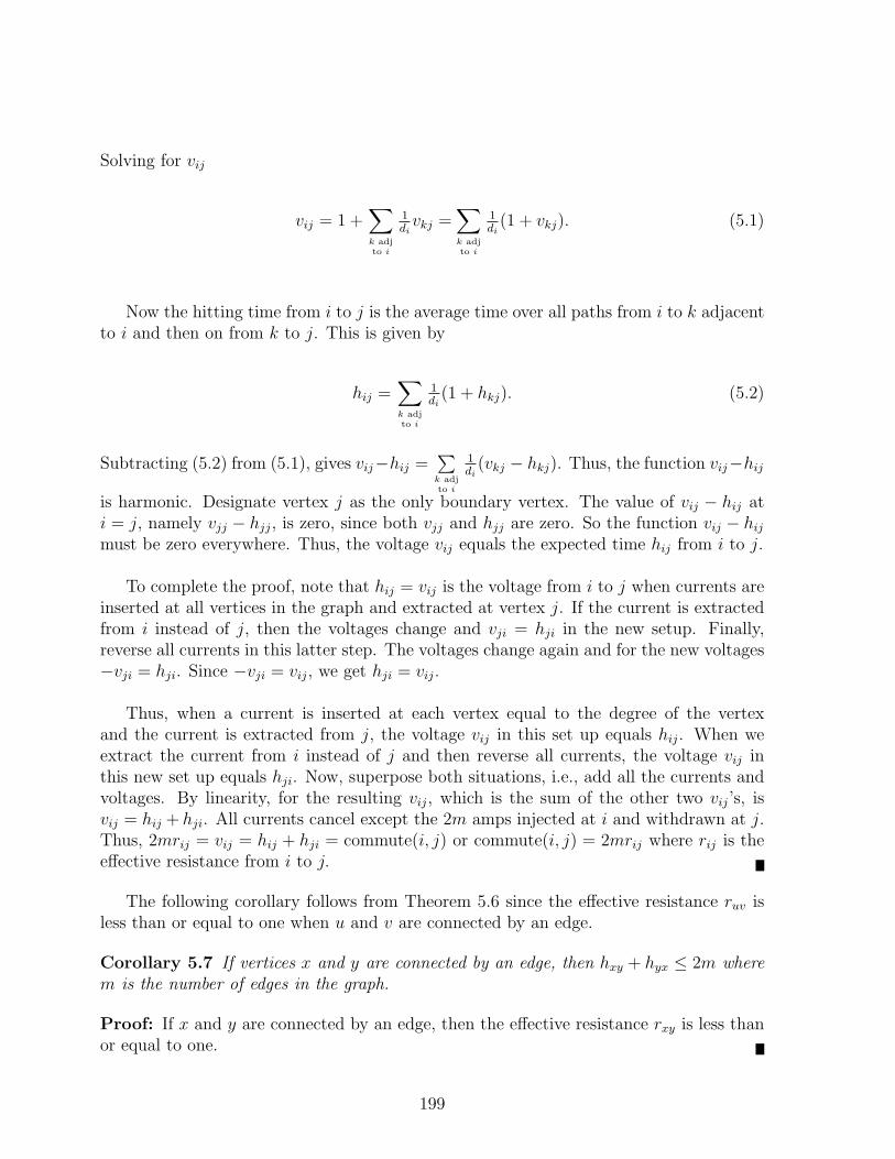
The commute time, commute(x, y), is the expected time of a random walk starting atx reaching y and then returning to x. So commute(x, y) = hxy + hyx. Think of goingfrom home to office and returning home. We now relate the commute time to an electricalquantity, the effective resistance. The effective resistance between two vertices x and y inan electrical network is the voltage difference between x and y when one unit of currentis inserted at vertex x and withdrawn from vertex y.

Theorem 5.6 Given an undirected graph, consider the electrical network where each edgeof the graph is replaced by a one ohm resistor. Given vertices x and y, the commute time,commute(x, y), equals 2mrxy where rxy is the effective resistance from x to y and m is thenumber of edges in the graph.

Proof: Insert at each vertex i a current equal to the degree di of vertex i. The totalcurrent inserted is 2m where m is the number of edges. Extract from a specific vertex jall of this 2m current. Let vij be the voltage difference from i to j. The current into idivides into the di resistors at vertex i. The current in each resistor is proportional to thevoltage across it. Let k be a vertex adjacent to i. Then the current through the resistorbetween i and k is vij − vkj, the voltage drop across the resister. The sum of the currentsout of i through the resisters must equal di, the current injected into i.

di =∑

k adj

to i

(vij − vkj) = divij −∑

k adj

to i

vkj.

198

Solving for vij

vij = 1 +∑

k adj

to i

1divkj =

∑

k adj

to i

1di(1 + vkj). (5.1)

Now the hitting time from i to j is the average time over all paths from i to k adjacentto i and then on from k to j. This is given by

hij =∑

k adj

to i

1di(1 + hkj). (5.2)

Subtracting (5.2) from (5.1), gives vij−hij =∑

k adj

to i

1di(vkj − hkj). Thus, the function vij−hij

is harmonic. Designate vertex j as the only boundary vertex. The value of vij − hij ati = j, namely vjj − hjj, is zero, since both vjj and hjj are zero. So the function vij − hij

must be zero everywhere. Thus, the voltage vij equals the expected time hij from i to j.

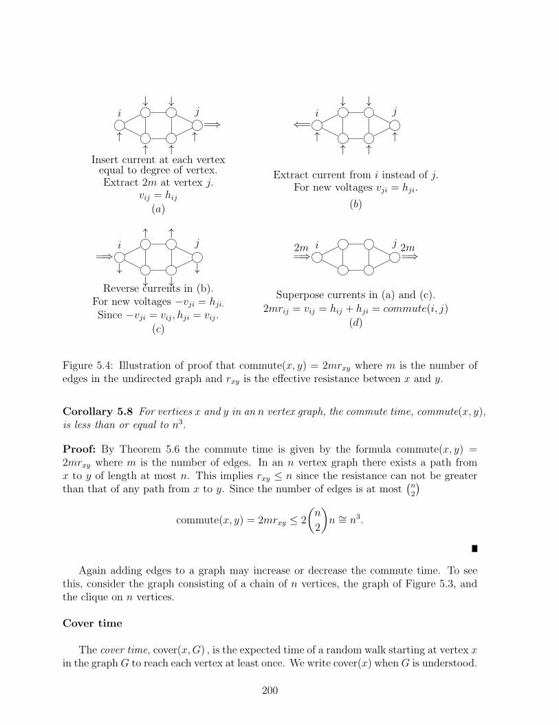
To complete the proof, note that hij = vij is the voltage from i to j when currents areinserted at all vertices in the graph and extracted at vertex j. If the current is extractedfrom i instead of j, then the voltages change and vji = hji in the new setup. Finally,reverse all currents in this latter step. The voltages change again and for the new voltages−vji = hji. Since −vji = vij, we get hji = vij.

Thus, when a current is inserted at each vertex equal to the degree of the vertexand the current is extracted from j, the voltage vij in this set up equals hij. When weextract the current from i instead of j and then reverse all currents, the voltage vij inthis new set up equals hji. Now, superpose both situations, i.e., add all the currents andvoltages. By linearity, for the resulting vij, which is the sum of the other two vij’s, isvij = hij + hji. All currents cancel except the 2m amps injected at i and withdrawn at j.Thus, 2mrij = vij = hij + hji = commute(i, j) or commute(i, j) = 2mrij where rij is theeffective resistance from i to j.

The following corollary follows from Theorem 5.6 since the effective resistance ruv isless than or equal to one when u and v are connected by an edge.

Corollary 5.7 If vertices x and y are connected by an edge, then hxy + hyx ≤ 2m wherem is the number of edges in the graph.

Proof: If x and y are connected by an edge, then the effective resistance rxy is less thanor equal to one.

199

i j

↑

↓

↑

↓

↑↑

=⇒

Insert current at each vertexequal to degree of vertex.Extract 2m at vertex j.

vij = hij

(a)

i j

↑

↓

↑

↓

↑↑

⇐=

Extract current from i instead of j.For new voltages vji = hji.

(b)

i j

↓

↑

↓

↑

↓↓

=⇒

Reverse currents in (b).For new voltages −vji = hji.

Since −vji = vij, hji = vij.

(c)

i j=⇒ =⇒2m 2m

Superpose currents in (a) and (c).2mrij = vij = hij + hji = commute(i, j)

(d)

Figure 5.4: Illustration of proof that commute(x, y) = 2mrxy where m is the number ofedges in the undirected graph and rxy is the effective resistance between x and y.

Corollary 5.8 For vertices x and y in an n vertex graph, the commute time, commute(x, y),is less than or equal to n3.

Proof: By Theorem 5.6 the commute time is given by the formula commute(x, y) =2mrxy where m is the number of edges. In an n vertex graph there exists a path fromx to y of length at most n. This implies rxy ≤ n since the resistance can not be greaterthan that of any path from x to y. Since the number of edges is at most

(n2

)

commute(x, y) = 2mrxy ≤ 2

(n

2

)

n ∼= n3.

Again adding edges to a graph may increase or decrease the commute time. To seethis, consider the graph consisting of a chain of n vertices, the graph of Figure 5.3, andthe clique on n vertices.

Cover time

The cover time, cover(x,G) , is the expected time of a random walk starting at vertex xin the graph G to reach each vertex at least once. We write cover(x) when G is understood.

200

The cover time of an undirected graph G, denoted cover(G), is

cover(G) = maxx

cover(x,G).

For cover time of an undirected graph, increasing the number of edges in the graphmay increase or decrease the cover time depending on the situation. Again consider threegraphs, a chain of length n which has cover time Θ(n2), the graph in Figure 5.3 which hascover time Θ(n3), and the complete graph on n vertices which has cover time Θ(n log n).Adding edges to the chain of length n to create the graph in Figure 5.3 increases thecover time from n2 to n3 and then adding even more edges to obtain the complete graphreduces the cover time to n log n.

Note: The cover time of a clique is θ(n log n) since this is the time to select everyinteger out of n integers with high probability, drawing integers at random. This is calledthe coupon collector problem. The cover time for a straight line is Θ(n2) since it is thesame as the hitting time. For the graph in Figure 5.3, the cover time is Θ(n3) since onetakes the maximum over all start states and cover(x,G) = Θ (n3) where x is the vertexof attachment.

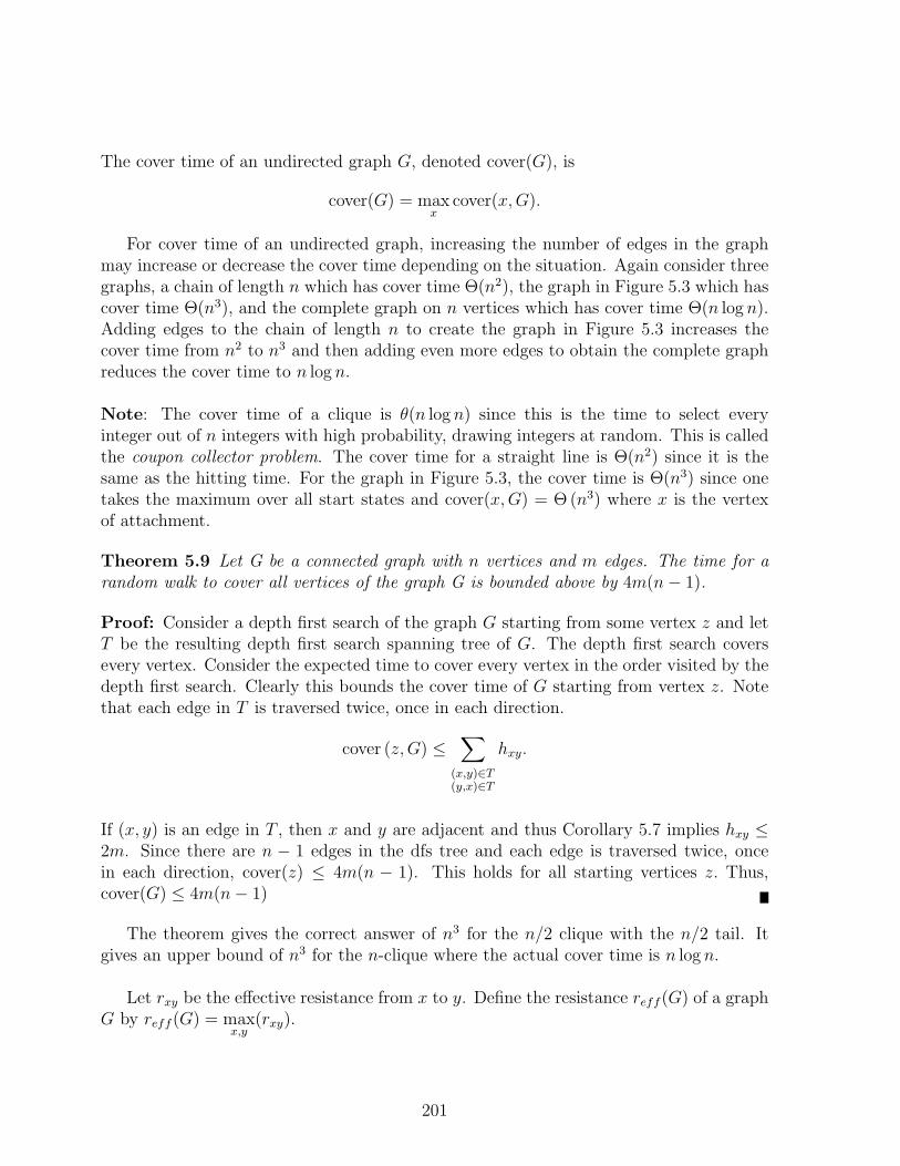
Theorem 5.9 Let G be a connected graph with n vertices and m edges. The time for arandom walk to cover all vertices of the graph G is bounded above by 4m(n− 1).

Proof: Consider a depth first search of the graph G starting from some vertex z and letT be the resulting depth first search spanning tree of G. The depth first search coversevery vertex. Consider the expected time to cover every vertex in the order visited by thedepth first search. Clearly this bounds the cover time of G starting from vertex z. Notethat each edge in T is traversed twice, once in each direction.

cover (z,G) ≤∑

(x,y)∈T(y,x)∈T

hxy.

If (x, y) is an edge in T , then x and y are adjacent and thus Corollary 5.7 implies hxy ≤2m. Since there are n − 1 edges in the dfs tree and each edge is traversed twice, oncein each direction, cover(z) ≤ 4m(n − 1). This holds for all starting vertices z. Thus,cover(G) ≤ 4m(n− 1)

The theorem gives the correct answer of n3 for the n/2 clique with the n/2 tail. Itgives an upper bound of n3 for the n-clique where the actual cover time is n log n.

Let rxy be the effective resistance from x to y. Define the resistance reff (G) of a graphG by reff (G) = max

x,y(rxy).

201

Theorem 5.10 Let G be an undirected graph with m edges. Then the cover time for Gis bounded by the following inequality

mreff (G) ≤ cover(G) ≤ 2e3mreff (G) lnn+ n

where e=2.71 is Euler’s constant and reff (G) is the resistance of G.

Proof: By definition reff (G) = maxx,y

(rxy). Let u and v be the vertices of G for which

rxy is maximum. Then reff (G) = ruv. By Theorem 5.6, commute(u, v) = 2mruv. Hencemruv = 1

2commute(u, v). Clearly the commute time from u to v and back to u is less

than twice the max(huv, hvu) and max(huv, hvu) is clearly less than the cover time of G.Putting these facts together gives the first inequality in the theorem.

mreff (G) = mruv =12commute(u, v) ≤ max(huv, hvu) ≤ cover(G)

For the second inequality in the theorem, by Theorem 5.6, for any x and y, commute(x, y)equals 2mrxy which is less than or equal to 2mreff (G), implying hxy ≤ 2mreff (G). Bythe Markov inequality, since the expected time to reach y starting at any x is less than2mreff (G), the probability that y is not reached from x in 2mreff (G)e3 steps is at most1e3. Thus, the probability that a vertex y has not been reached in 2e3mreff (G) log n steps

is at most 1e3

lnn= 1

n3 because a random walk of length 2e3mr(G) log n is a sequence oflog n independent random walks, each of length 2e3mr(G)reff (G). Suppose after a walkof 2e3mreff (G) log n steps, vertices v1, v2, . . . , vl had not been reached. Walk until v1 isreached, then v2, etc. By Corollary 5.8 the expected time for each of these is n3, but sinceeach happens only with probability 1/n3, we effectively take O(1) time per vi, for a totaltime at most n. More precisely,

cover(G) ≤ 2e3mreff (G) log n+∑

v

Prob(v was not visited in the first 2e3mreff (G) steps

)n3

≤ 2e3mreff (G) log n+∑

v

1

n3n3 ≤ 2e3mreff (G) + n.

5.4 Random Walks in Euclidean Space

Many physical processes such as Brownian motion are modeled by random walks.Random walks in Euclidean d-space consisting of fixed length steps parallel to the coor-dinate axes are really random walks on a d-dimensional lattice and are a special case ofrandom walks on graphs. In a random walk on a graph, at each time unit an edge fromthe current vertex is selected at random and the walk proceeds to the adjacent vertex.We begin by studying random walks on lattices.

Random walks on lattices

202

We now apply the analogy between random walks and current to lattices. Considera random walk on a finite segment −n, . . . ,−1, 0, 1, 2, . . . , n of a one dimensional latticestarting from the origin. Is the walk certain to return to the origin or is there some prob-ability that it will escape, i.e., reach the boundary before returning? The probability ofreaching the boundary before returning to the origin is called the escape probability. Weshall be interested in this quantity as n goes to infinity.

Convert the lattice to an electrical network by replacing each edge with a one ohmresister. Then the probability of a walk starting at the origin reaching n or –n beforereturning to the origin is the escape probability given by

pescape =ceffca

where ceff is the effective conductance between the origin and the boundary points and cais the sum of the conductance’s at the origin. In a d-dimensional lattice, ca = 2d assumingthat the resistors have value one. For the d-dimensional lattice

pescape =1

2d reff

In one dimension, the electrical network is just two series connections of n one ohm re-sistors connected in parallel. So as n goes to infinity, reff goes to infinity and the escapeprobability goes to zero as n goes to infinity. Thus, the walk in the unbounded one dimen-sional lattice will return to the origin with probability one. This is equivalent to flippinga balanced coin and keeping tract of the number of heads minus the number of tails. Thecount will return to zero infinitely often. By the law of large numbers in n steps withhigh probability the walk will be within

√n distance of the origin.

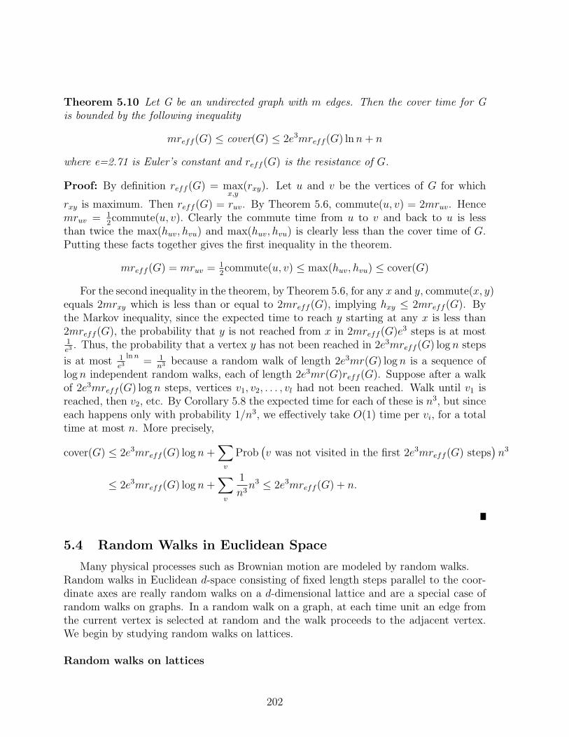
Two dimensions

For the 2-dimensional lattice, consider a larger and larger square about the origin forthe boundary as shown in Figure 5.5a and consider the limit of reff as the squares getlarger. Shorting the resistors on each square can only reduce reff . Shorting the resistorsresults in the linear network shown in Figure 5.5b. As the paths get longer, the numberof resistors in parallel also increases. The resistor between vertex i and i + 1 is really4(2i+1) unit resistors in parallel. The effective resistance of 4(2i+1) resistors in parallelis 1/4(2i+ 1). Thus,

reff ≥ 14+ 1

12+ 1

20+ · · · = 1

4(1 + 1

3+ 1

5+ · · · ) = Θ(lnn).

Since the lower bound on the effective resistance and hence the effective resistance goesto infinity, the escape probability goes to zero for the 2-dimensional lattice.

Three dimensions

203

(a)

4 12 20

0 1 2 3

Number of resistorsin parallel

(b)

Figure 5.5: 2-dimensional lattice along with the linear network resulting from shortingresistors on the concentric squares about the origin.

In three dimensions, the resistance along any path to infinity grows to infinity butthe number of paths in parallel also grows to infinity. It turns out there are a sufficientnumber of paths that reff remains finite and thus there is a nonzero escape probability.We will prove this now. First note that shorting any edge decreases the resistance, sowe do not use shorting in this proof, since we seek to prove an upper bound on theresistance. Instead we remove some edges, which increases their resistance to infinity andhence increases the effective resistance, giving an upper bound. To simplify things weconsider walks on on quadrant rather than the full grid. The resistance to infinity derivedfrom only the quadrant is an upper bound on the resistance of the full grid.

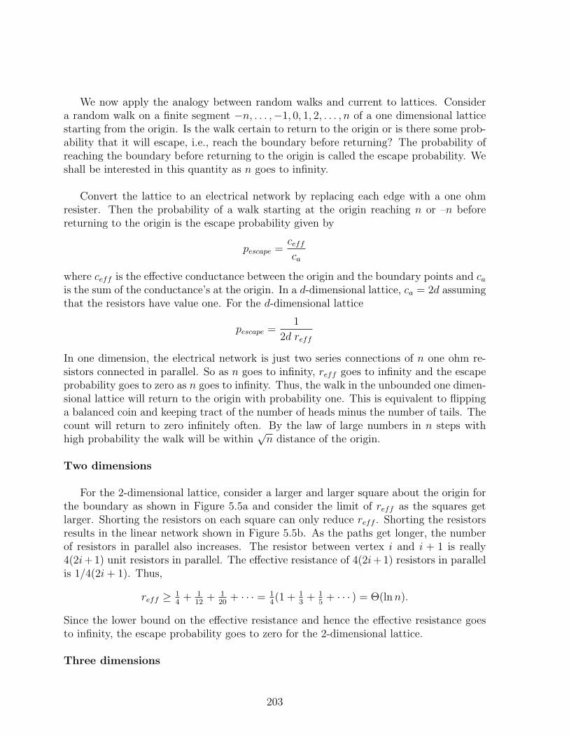
The construction used in three dimensions is easier to explain first in two dimensions.Draw dotted diagonal lines at x+ y = 2n−1. Consider two paths that start at the origin.One goes up and the other goes to the right. Each time a path encounters a dotteddiagonal line, split the path into two, one which goes right and the other up. Wheretwo paths cross, split the vertex into two, keeping the paths separate. By a symmetryargument, splitting the vertex does not change the resistance of the network. Removeall resistors except those on these paths. The resistance of the original network is lessthan that of the tree produced by this process since removing a resistor is equivalent toincreasing its resistance to infinity.

The distances between splits increase and are 1, 2, 4, etc. At each split the numberof paths in parallel doubles. See Figure 5.7. Thus, the resistance to infinity in this twodimensional example is

1

2+

1

42 +

1

84 + · · · = 1

2+

1

2+

1

2+ · · · = ∞.

204

y

x1 3 7

1

3

7

Figure 5.6: Paths in a 2-dimensional lattice obtained from the 3-dimensional constructionapplied in 2-dimensions.

In the analogous three dimensional construction, paths go up, to the right, and out ofthe plane of the paper. The paths split three ways at planes given by x+ y + z = 2n − 1.Each time the paths split the number of parallel segments triple. Segments of the pathsbetween splits are of length 1, 2, 4, etc. and the resistance of the segments are equal tothe lengths. The resistance out to infinity for the tree is

13+ 1

92 + 1

274 + · · · = 1

3

(1 + 2

3+ 4

9+ · · ·

)= 1

31

1−23

= 1

The resistance of the three dimensional lattice is less. It is important to check that thepaths are edge-disjoint and so the tree is a subgraph of the lattice. Going to a subgraph isequivalent to deleting edges which only increases the resistance. That is why the resistanceof the lattice is less than that of the tree. Thus, in three dimensions the escape probabilityis nonzero. The upper bound on reff gives the lower bound

pescape =12d

1reff

≥ 16.

205

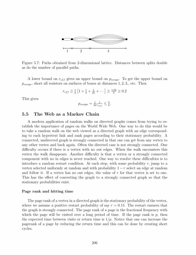
1 2 4

Figure 5.7: Paths obtained from 2-dimensional lattice. Distances between splits doubleas do the number of parallel paths.

A lower bound on reff gives an upper bound on pescape. To get the upper bound onpescape, short all resistors on surfaces of boxes at distances 1, 2, 3,, etc. Then

reff ≥ 16

[1 + 1

9+ 1

25+ · · ·

]≥ 1.23

6≥ 0.2

This givespescape =

12d

1reff

≤ 56.

5.5 The Web as a Markov Chain

A modern application of random walks on directed graphs comes from trying to es-tablish the importance of pages on the World Wide Web. One way to do this would beto take a random walk on the web viewed as a directed graph with an edge correspond-ing to each hypertext link and rank pages according to their stationary probability. Aconnected, undirected graph is strongly connected in that one can get from any vertex toany other vertex and back again. Often the directed case is not strongly connected. Onedifficulty occurs if there is a vertex with no out edges. When the walk encounters thisvertex the walk disappears. Another difficulty is that a vertex or a strongly connectedcomponent with no in edges is never reached. One way to resolve these difficulties is tointroduce a random restart condition. At each step, with some probability r, jump to avertex selected uniformly at random and with probability 1− r select an edge at randomand follow it. If a vertex has no out edges, the value of r for that vertex is set to one.This has the effect of converting the graph to a strongly connected graph so that thestationary probabilities exist.

Page rank and hitting time

The page rank of a vertex in a directed graph is the stationary probability of the vertex,where we assume a positive restart probability of say r = 0.15. The restart ensures thatthe graph is strongly connected. The page rank of a page is the fractional frequency withwhich the page will be visited over a long period of time. If the page rank is p, thenthe expected time between visits or return time is 1/p. Notice that one can increase thepagerank of a page by reducing the return time and this can be done by creating shortcycles.

206

ijpji

120.85πi

120.85πi

0.15πj 0.15πi

πi = 0.85πjpji +0.852πi

πi = 1.48πjpji

Figure 5.8: Impact on page rank of adding a self loop

Consider a vertex i with a single edge in from vertex j and a single edge out. Thestationary probability π satisfies πP = π, and thus

πi = πjpji.

Adding a self-loop at i, results in a new equation

πi = πjpji +1

2πi

orπi = 2 πjpji.

Of course, πj would have changed too, but ignoring this for now, pagerank is doubled bythe addition of a self-loop. Adding k self loops, results in the equation

πi = πjpji +k

k + 1πi,

and again ignoring the change in πj, we now have πi = (k + 1)πjpji. What preventsone from increasing the page rank of a page arbitrarily? The answer is the restart. Weneglected the 0.15 probability that is taken off for the random restart. With the restarttaken into account, the equation for πi when there is no self-loop is

πi = 0.85πjpji

whereas, with k self-loops, the equation is

πi = 0.85πjpji + 0.85k

k + 1πi.

Solving for πi yields

πi =0.85k + 0.85

0.15k + 1πjpji

which for k = 1 is πi = 1.48πjPji and in the limit as k → ∞ is πi = 5.67πjpji. Adding asingle loop only increases pagerank by a factor of 1.74 and adding k loops increases it byat most a factor of 6.67 for arbitrarily large k.

207

Hitting time

Related to page rank is a quantity called hitting time. Hitting time is closely relatedto return time and thus to the reciprocal of page rank. One way to return to a vertexv is by a path in the graph from v back to v. Another way is to start on a path thatencounters a restart, followed by a path from the random restart vertex to v. The timeto reach v after a restart is the hitting time. Thus, return time is clearly less than theexpected time until a restart plus hitting time. The fastest one could return would be ifthere were only paths of length two since self loops are ignored in calculating page rank. Ifr is the restart value, then the loop would be traversed with at most probability (1− r)2.With probability r + (1− r) r = (2− r) r one restarts and then hits v. Thus, the returntime is at least 2 (1− r)2+(2− r) r× (hitting time). Combining these two bounds yields

2 (1− r)2 + (2− r) rE (hitting time) ≤ E (return time) ≤ E (hitting time) .

The relationship between return time and hitting time can be used to see if a vertex hasunusually high probability of short loops. However, there is no efficient way to computehitting time for all vertices as there is for return time. For a single vertex v, one can com-pute hitting time by removing the edges out of the vertex v for which one is computinghitting time and then run the page rank algorithm for the new graph. The hitting timefor v is the reciprocal of the page rank in the graph with the edges out of v removed.Since computing hitting time for each vertex requires removal of a different set of edges,the algorithm only gives the hitting time for one vertex at a time. Since one is probablyonly interested in the hitting time of vertices with low hitting time, an alternative wouldbe to use a random walk to estimate the hitting time of low hitting time vertices.

Spam

Suppose one has a web page and would like to increase its page rank by creating someother web pages with pointers to the original page. The abstract problem is the following.We are given a directed graph G and a vertex v whose page rank we want to increase.We may add new vertices to the graph and add edges from v or from the new verticesto any vertices we want. We cannot add edges out of other vertices. We can also deleteedges from v.

The page rank of v is the stationary probability for vertex v with random restarts. Ifwe delete all existing edges out of v, create a new vertex u and edges (v, u) and (u, v),then the page rank will be increased since any time the random walk reaches v it willbe captured in the loop v → u → v. A search engine can counter this strategy by morefrequent random restarts.

A second method to increase page rank would be to create a star consisting of thevertex v at its center along with a large set of new vertices each with a directed edge to

208

v. These new vertices will sometimes be chosen as the target of the random restart andhence the vertices increase the probability of the random walk reaching v. This secondmethod is countered by reducing the frequency of random restarts.

Notice that the first technique of capturing the random walk increases page rank butdoes not effect hitting time. One can negate the impact of someone capturing the randomwalk on page rank by increasing the frequency of random restarts. The second techniqueof creating a star increases page rank due to random restarts and decreases hitting time.One can check if the page rank is high and hitting time is low in which case the pagerank is likely to have been artificially inflated by the page capturing the walk with shortcycles.

Personalized page rank

In computing page rank, one uses a restart probability, typically 0.15, in which at eachstep, instead of taking a step in the graph, the walk goes to a vertex selected uniformlyat random. In personalized page rank, instead of selecting a vertex uniformly at random,one selects a vertex according to a personalized probability distribution. Often the distri-bution has probability one for a single vertex and whenever the walk restarts it restartsat that vertex.

Algorithm for computing personalized page rank

First, consider the normal page rank. Let α be the restart probability with whichthe random walk jumps to an arbitrary vertex. With probability 1− α the random walkselects a vertex uniformly at random from the set of adjacent vertices. Let p be a rowvector denoting the page rank and let G be the adjacency matrix with rows normalizedto sum to one. Then

p = αn(1, 1, . . . , 1) + (1− α)pG

p[I − (1− α)G] =α

n(1, 1, . . . , 1)

orp = α

n(1, 1, . . . , 1) [I − (1− α)G]−1.

Thus, in principle, p can be found by computing the inverse of [I − (1 − α)G]−1. Butthis is far from practical since for the whole web one would be dealing with matrices withbillions of rows and columns. A more practical procedure is to run the random walk andobserve using the basics of the power method in Chapter 3 that the process converges tothe solution p.

For the personalized page rank, instead of restarting at an arbitrary vertex, the walkrestarts at a designated vertex. More generally, it may restart in some specified neighbor-hood. Suppose the restart selects a vertex using the probability distribution s. Then, in

209

the above calculation replace the vector 1n(1, 1, . . . , 1) by the vector s. Again, the compu-

tation could be done by a random walk. But, we wish to do the random walk calculationfor personalized pagerank quickly since it is to be performed repeatedly. With more carethis can be done, though we do not describe it here.

5.6 Markov Chain Monte Carlo

The Markov Chain Monte Carlo (MCMC) method is a technique for sampling a mul-tivariate probability distribution p(x), where x = (x1, x2, . . . , xd). The MCMC method isused to estimate the expected value of a function f(x)

E(f) =∑

x

f(x)p(x).

If each xi can take on two or more values, then there are at least 2d values for x, so anexplicit summation requires exponential time. Instead, one could draw a set of samples,each sample x with probability p(x). Averaging f over these samples provides an estimateof the sum.

To sample according to p(x), design a Markov Chain whose states correspond to thepossible values of x and whose stationary probability distribution is p(x). There are twogeneral techniques to design such a Markov Chain: the Metropolis-Hastings algorithmand Gibbs sampling. The Fundamental Theorem of Markov Chains, Theorem 5.2, statesthat the average of f over states seen in a sufficiently long run is a good estimate of E(f).The harder task is to show that the number of steps needed before the long-run averageprobabilities are close to the stationary distribution grows polynomially in d, though thetotal number of states may grow exponentially in d. This phenomenon known as rapidmixing happens for a number of interesting examples. Section 5.8 presents a crucial toolused to show rapid mixing.

We used x ∈ Rd to emphasize that distributions are multi-variate. From a Markovchain perspective, each value x can take on is a state, i.e., a vertex of the graph on whichthe random walk takes place. Henceforth, we will use the subscripts i, j, k, . . . to denotestates and will use pi instead of p(x1, x2, . . . , xd) to denote the probability of the statecorresponding to a given set of values for the variables. Recall that in the Markov chainterminology, vertices of the graph are called states.

Recall the notation that p(t) is the row vector of probabilities of the random walkbeing at each state (vertex of the graph) at time t. So, p(t) has as many components as

there are states and its ith component, p(t)i , is the probability of being in state i at time

t. Recall the long-term t-step average is

a(t) =1

t

[p(0) + p(1) + · · ·+ p(t−1)

]. (5.3)

210

The expected value of the function f under the probability distribution p is E(f) =∑

i fipi where fi is the value of f at state i. Our estimate of this quantity will be theaverage value of f at the states seen in a t step walk. Call this estimate a. Clearly, theexpected value of a is

E(a) =∑

i

fi

(

1

t

t∑

j=1

Prob (walk is in state i at time j)

)

=∑

i

fia(t)i .

The expectation here is with respect to the “coin tosses” of the algorithm, not with respectto the underlying distribution p. Let fmax denote the maximum absolute value of f . It iseasy to see that

∣∣∣∣∣

∑

i

fipi − E(a)

∣∣∣∣∣≤ fmax

∑

i

|pi − a(t)i | = fmax|p− a(t)|1 (5.4)

where the quantity |p − a(t)|1 is the l1 distance between the probability distributions pand a(t) and is often called the “total variation distance” between the distributions. Wewill build tools to upper bound |p−a(t)|1. Since p is the stationary distribution, the t forwhich |p − a(t)|1 becomes small is determined by the rate of convergence of the Markovchain to its steady state.

The following proposition is often useful.

Proposition 5.11 For two probability distributions p and q,

|p− q|1 = 2∑

i

(pi − qi)+ = 2

∑

i

(qi − pi)+

where x+ = x if x ≥ 0 and x+ = 0 if x < 0.

The proof is left as an exercise.

5.6.1 Metropolis-Hasting Algorithm

The Metropolis-Hasting algorithm is a general method to design a Markov chain whosestationary distribution is a given target distribution p. Start with a connected undirectedgraph G on the set of states. If the states are the lattice points (x1, x2, . . . , xd) in Rd withxi ∈ 0, 1, 2, , . . . , n, then G is the lattice graph with 2d coordinate edges at each interiorvertex. In general, let r be the maximum degree of any vertex of G. The transitions ofthe Markov chain are defined as follows. At state i select neighbor j with probability 1

r.

Since the degree of i may be less than r, with some probability no edge is selected and thewalk remains at i. If a neighbor j is selected and pj ≥ pi, go to j. If pj < pi, go to j withprobability pj/pi and stay at i with probability 1 − pj

pi. Intuitively, this favors “heavier”

states with higher p values. So, for i 6= j, adjacent in G,

pij =1

rmin

(

1,pjpi

)

211

d

a

c

b

18

12

18

14

p(a) = 12

p(b) = 14

p(c) = 18

p(d) = 18

a → b 13

14

21= 1

6c → a 1

3

a → c 13

18

21= 1

12c → b 1

3

a → d 13

18

21= 1

12c → d 1

3

a → a 1− 16− 1

12− 1

12= 2

3c → c 1− 1

3− 1

3− 1

3= 0

b → a 13

d → a 13

b → c 13

18

41= 1

6d → c 1

3

b → b 1− 13− 1

6= 1

2d → d 1− 1

3− 1

3= 1

3

p(a) = p(a)p(a → a) + p(b)p(b → a) + p(c)p(c → a) + p(d)p(d → a)= 1

223+ 1

413+ 1

813+ 1

813= 1

2

p(b) = p(a)p(a → b) + p(b)p(b → b) + p(c)p(c → b)= 1

216+ 1

412+ 1

813= 1

4

p(c) = p(a)p(a → c) + p(b)p(b → c) + p(c)p(c → c) + p(d)p(d → c)= 1

2112

+ 14

16+ 1

80 + 1

813= 1

8

p(d) = p(a)p(a → d) + p(c)p(c → d) + p(d)p(d → d)= 1

2112

+ 18

13+ 1

813= 1

8

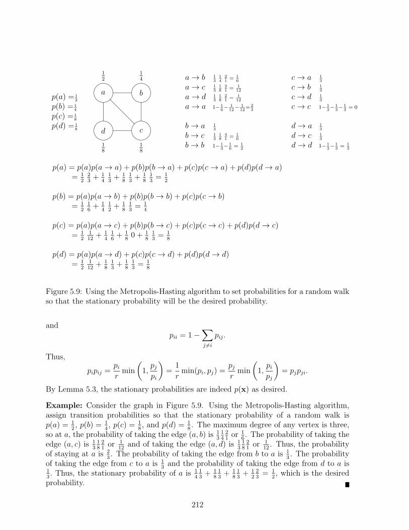
Figure 5.9: Using the Metropolis-Hasting algorithm to set probabilities for a random walkso that the stationary probability will be the desired probability.

andpii = 1−

∑

j 6=i

pij.

Thus,

pipij =pirmin

(

1,pjpi

)

=1

rmin(pi, pj) =

pjrmin

(

1,pipj

)

= pjpji.

By Lemma 5.3, the stationary probabilities are indeed p(x) as desired.

Example: Consider the graph in Figure 5.9. Using the Metropolis-Hasting algorithm,assign transition probabilities so that the stationary probability of a random walk isp(a) = 1

2, p(b) = 1

4, p(c) = 1

8, and p(d) = 1

8. The maximum degree of any vertex is three,

so at a, the probability of taking the edge (a, b) is 131421or 1

6. The probability of taking the

edge (a, c) is 131821or 1

12and of taking the edge (a, d) is 1

31821or 1

12. Thus, the probability

of staying at a is 23. The probability of taking the edge from b to a is 1

3. The probability

of taking the edge from c to a is 13and the probability of taking the edge from d to a is

13. Thus, the stationary probability of a is 1

413+ 1

813+ 1

813+ 1

223= 1

2, which is the desired

probability.

212

5.6.2 Gibbs Sampling

Gibbs sampling is another Markov Chain Monte Carlo method to sample from amultivariate probability distribution. Let p (x) be the target distribution where x =(x1, . . . , xd). Gibbs sampling consists of a random walk on an undirectd graph whosevertices correspond to the values of x = (x1, . . . , xd) and in which there is an edge fromx to y if x and y differ in only one coordinate. Thus, the underlying graph is like ad-dimensional lattice except that the vertices in the same coordinate line form a clique.

To generate samples of x = (x1, . . . , xd) with a target distribution p (x), the Gibbssampling algorithm repeats the following steps. One of the variables xi is chosen to beupdated. Its new value is chosen based on the marginal probability of xi with the othervariables fixed. There are two commonly used schemes to determine which xi to update.One scheme is to choose xi randomly, the other is to choose xi by sequentially scanningfrom x1 to xd.

Suppose that x and y are two states that differ in only one coordinate. Without lossof generality let that coordinate be the first. Then, in the scheme where a coordinate israndomly chosen to modify, the probability pxy of going from x to y is

pxy =1

dp(y1|x2, x3, . . . , xd).

Simplify followingThe normalizing constant is 1/d since for a given value i the proba-bility distribution of p(yi|x1, x2, . . . , xi−1, xi+1, . . . , xd) sums to one, and thus summing iover the d-dimensions results in a value of d. Similarly,

pyx =1

dp(x1|y2, y3, . . . , yd)

=1

dp(x1|x2, x3, . . . , xd).

Here use was made of the fact that for j 6= i, xj = yj.

It is simple to see that this chain has stationary probability proportional to p (x).Rewrite pxy as

pxy =1

d

p(y1|x2, x3, . . . , xd)p(x2, x3, . . . , xd)

p(x2, x3, . . . , xd)

=1

d

p(y1, x2, x3, . . . , xd)

p(x2, x3, . . . , xd)

=1

d

p(y)

p(x2, x3, . . . , xd)

again using xj = yj for j 6= i. Similarly write

pyx =1

d

p(x)

p(x2, x3, . . . , xd)

213

1,1 1,2 1,3

2,1 2,2 2,3

3,1 3,2 3,3

58

712

13

34

38

512

16

16

112

18

16

112

13

14

16

p(1, 1) = 13

p(1, 2) = 14

p(1, 3) = 16

p(2, 1) = 18

p(2, 2) = 16

p(2, 3) = 112

p(3, 1) = 16

p(3, 2) = 16

p(3, 3) = 112

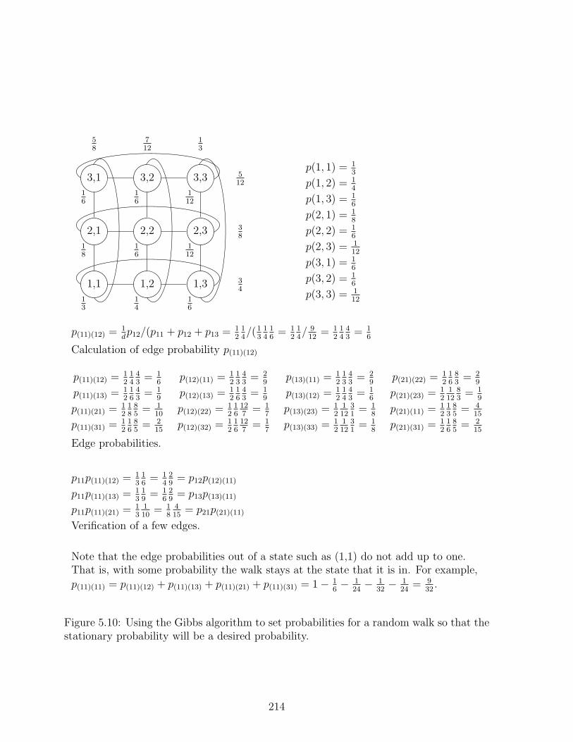
p(11)(12) =1dp12/(p11 + p12 + p13 =

1214/(1

31416= 1

214/ 912

= 121443= 1

6

Calculation of edge probability p(11)(12)

p(11)(12) =121443= 1

6

p(11)(13) =121643= 1

9

p(11)(21) =121885= 1

10

p(11)(31) =121685= 2

15

p(12)(11) =121343= 2

9

p(12)(13) =121643= 1

9

p(12)(22) =1216127= 1

7

p(12)(32) =1216127= 1

7

p(13)(11) =121343= 2

9

p(13)(12) =121443= 1

6

p(13)(23) =12

112

31= 1

8

p(13)(33) =12

112

31= 1

8

p(21)(22) =121683= 2

9

p(21)(23) =12

112

83= 1

9

p(21)(11) =121385= 4

15

p(21)(31) =121685= 2

15

Edge probabilities.

p11p(11)(12) =1316= 1

429= p12p(12)(11)

p11p(11)(13) =1319= 1

629= p13p(13)(11)

p11p(11)(21) =13

110

= 18

415

= p21p(21)(11)

Verification of a few edges.

Note that the edge probabilities out of a state such as (1,1) do not add up to one.That is, with some probability the walk stays at the state that it is in. For example,

p(11)(11) = p(11)(12) + p(11)(13) + p(11)(21) + p(11)(31) = 1− 16− 1

24− 1

32− 1

24= 9

32.

Figure 5.10: Using the Gibbs algorithm to set probabilities for a random walk so that thestationary probability will be a desired probability.

214

from which it follows that p(x)pxy = p(y)pyx. By Lemma 5.3 the stationary probabilityof the random walk is p(x).

5.7 Areas and Volumes

Computing areas and volumes is a classical problem. For many regular figures intwo and three dimensions there are closed form formulae. In Chapter 2, we saw how tocompute volume of a high dimensional sphere by integration. For general convex sets ind-space, there are no closed form formulae. Can we estimate volumes of d-dimensionalconvex sets in time that grows as a polynomial function of d? The MCMC method answesthis question in the affirmative.

One way to estimate the area of the region is to enclose it in a rectangle and estimatethe ratio of the area of the region to the area of the rectangle by picking random pointsin the rectangle and seeing what proportion land in the region. Such methods fail in highdimensions. Even for a sphere in high dimension, a cube enclosing the sphere has expo-nentially larger area, so exponentially many samples are required to estimate the volumeof the sphere.

It turns out that the problem of estimating volumes of sets is reducible to the problemof drawing uniform random samples from sets. Suppose one wants to estimate the volumeof a convex set R. Create a concentric series of larger and larger spheres S1, S2, . . . , Sk

such that S1 is contained in R and Sk contains R. Then

Vol(R) = Vol(Sk ∩R) =Vol(Sk ∩R)

Vol(Sk−1 ∩R)

Vol(Sk−1 ∩R)

Vol(Sk−2 ∩R)· · · Vol(S2 ∩R)

Vol(S1 ∩R)Vol(S1)

If the radius of the sphere Si is 1 +1dtimes the radius of the sphere Si−1, then the value

ofVol(Sk−1 ∩R)

Vol(Sk−2 ∩R)

can be estimated by rejection sampling provided one can select points at random from ad-dimensional region. Since the radii of the spheres grows as 1+ 1

d, the number of spheres

is at mostO(log1+(1/d) R) = O(Rd).

It remains to show how to draw a uniform random sample from a d-dimensional set.It is at this point that we require the set to be convex so that the Markov chain techniquewe use will converge quickly to its stationary probability. To select a random sample froma d-dimensional convex set impose a grid on the region and do a random walk on the gridpoints. At each time, pick one of the 2d coordinate neighbors of the current grid point,each with probability 1/(2d) and go to the neighbor if it is still in the set; otherwise, stayput and repeat. If the grid length in each of the d coordinate directions is at most somea, the total number of grid points in the set is at most ad. Although this is exponential in

215

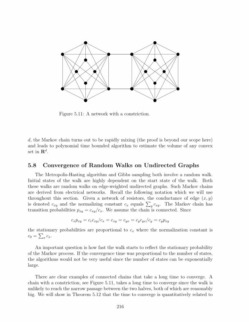
Figure 5.11: A network with a constriction.

d, the Markov chain turns out to be rapidly mixing (the proof is beyond our scope here)and leads to polynomial time bounded algorithm to estimate the volume of any convexset in Rd.

5.8 Convergence of Random Walks on Undirected Graphs

The Metropolis-Hasting algorithm and Gibbs sampling both involve a random walk.Initial states of the walk are highly dependent on the start state of the walk. Boththese walks are random walks on edge-weighted undirected graphs. Such Markov chainsare derived from electrical networks. Recall the following notation which we will usethroughout this section. Given a network of resistors, the conductance of edge (x, y)is denoted cxy and the normalizing constant cx equals

∑

y cxy. The Markov chain hastransition probabilities pxy = cxy/cx. We assume the chain is connected. Since

cxpxy = cccxy/cx = cxy = cyx = cycyx/cy = cypxy

the stationary probabilities are proportional to cx where the normalization constant isc0 =

∑

x cx.

An important question is how fast the walk starts to reflect the stationary probabilityof the Markov process. If the convergence time was proportional to the number of states,the algorithms would not be very useful since the number of states can be exponentiallylarge.

There are clear examples of connected chains that take a long time to converge. Achain with a constriction, see Figure 5.11, takes a long time to converge since the walk isunlikely to reach the narrow passage between the two halves, both of which are reasonablybig. We will show in Theorem 5.12 that the time to converge is quantitatively related to

216

the tightest constriction.

A function is unimodal if it has a single maximum, i.e., it increases and then decreases.A unimodal function like the normal density has no constriction blocking a random walkfrom getting out of a large set of states, whereas a bimodal function can have a con-striction. Interestingly, many common multivariate distributions as well as univariateprobability distributions like the normal and exponential are unimodal and sampling ac-cording to these distributions can be done using the methods here.

A natural problem is estimating the probability of a convex region in d-space accordingto a normal distribution. One technique to do this is rejection sampling. Let R be theregion defined by the inequality x1 + x2 + · · · + xd/2 ≤ xd/2+1 + · · · + xd. Pick a sampleaccording to the normal distribution and accept the sample if it satisfies the inequality. Ifnot, reject the sample and retry until one gets a number of samples satisfying the inequal-ity. The probability of the region is approximated by the fraction of the samples thatsatisfied the inequality. However, suppose R was the region x1+x2+ · · ·+xd−1 ≤ xd. Theprobability of this region is exponentially small in d and so rejection sampling runs intothe problem that we need to pick exponentially many samples before we accept even onesample. This second situation is typical. Imagine computing the probability of failure ofa system. The object of design is to make the system reliable, so the failure probability islikely to be very low and rejection sampling will take a long time to estimate the failureprobability.

In general, there could be constrictions that prevent rapid convergence of a Markovchain to its stationary probability. However, if the set is convex in any number of dimen-sions, then there are no constrictions and there is rapid convergence although the proofof this is beyond the scope of this book.

We define below a combinatorial measure of constriction for a Markov chain, called thenormalized conductance, and relate this quantity to the rate at which the chain convergesto the stationarity probability. The conductance of an edge (x, y) leaving a set of statesS is defined to be πxcxy where πx is the stationary probability of vertex x. One way toavoid constrictions like the one in the picture of Figure 5.11 is to insure that the totalconductance of edges leaving every subset of states to be high. This is not possible if Swas itself small or even empty. So, in what follows, we “normalize” the total conductanceof edges leaving S by the size of S as measured by total cx for x ∈ S. Recall that pxy =

cxycx

and the stationary probability πx = cxc0

where c0 =∑

x cx. In defining the conductance ofedges leaving a set we have ignored the normalizing constants.

Definition 5.1 For a subset S of vertices, the normalized conductance Φ(S) of S is the

217

ratio of the total conductance of all edges from S to S to the total of the cx for x ∈ S.

Φ(S) =

∑

(x,y)

cxy

∑

x∈S

cx=

∑

(x,y)

cxpxy

∑

x∈S

c0πx

=

∑

(x,y)

c0πxpxy

∑

x∈S

c0πx

=

∑

(x,y)

πxpxy

∑

x∈S

πx

The normalized conductance5 of S is the probability of taking a step from S to outsideS conditioned on starting in S in the stationary probability distribution π. The stationarydistribution for state x conditioned on being in S is

πx

π(S)=

cx∑

x∈S

cx.

where π(S) =∑

x∈S

πx.

Definition 5.2 The normalized conductance of the Markov chain, denoted Φ, is definedby

Φ = minS

π(S)≤1/2

Φ(S).

The restriction to sets with π ≤ 1/2 in the definition of Φ is natural. The definition ofΦ guarantees that if Φ is high, there is high probability of moving from S to S so it isunlikely to get stuck in S provided π(S) ≤ 1

2. If π(S) > 1

2, say π(S) = 3

4, then since for

every edge πipij = πjpji

Φ(S) =

∑

i∈S πipij∑

i∈S πi

=

∑

j∈S πjpji

3∑

j∈S πk

= Φ(S)/3

Since Φ(S) ≥ Φ , we still have at least Φ/3 probability of moving out of S. The largerπ(S) is the smaller the probability of moving out, which is as it should be. We cannotmove out of the whole set! One does not need to escape from big sets. Note that aconstriction would mean a small Φ.

Definition 5.3 Fix ε > 0. The ε-mixing time of a Markov chain is the minimum integer tsuch that for any starting distribution p(0), the 1-norm distance between the t-step runningaverage probability distribution6 and the stationary distribution is at most ε.

5We will often drop the word “normalized” and just say “conductance”.6Recall that a(t) = 1

t(p(0) + p

(1) + · · ·+ p(t−1)) is called the running average distribution.

218

The theorem below states that if Φ, the normalized conductance of the Markov chain,is large, then there is fast convergence of the running average probability. Intuitively, ifΦ is large, the walk rapidly leaves any subset of states. Later we will see examples wherethe mixing time is much smaller than the cover time. That is, the number of steps beforea random walk reaches a random state independent of its starting state is much smallerthan the average number of steps needed to reach every state. In fact for some graphs,called expenders, the mixing time is logarithmic in the number of states.

Theorem 5.12 The ε-mixing time of a random walk on an undirected graph is

O

(ln(1/πmin)

Φ2ε3

)

where πmin is the minimum stationary probability of any state.

Proof: Let

t =c ln(1/πmin)

Φ2ε2,

for a suitable constant c. Let a = a(t) be the running average distribution for this valueof t. We need to show that |a− π| ≤ ε.

Let vi denote the ratio of the long term average probability for state i at time t di-vided by the stationary probability for state i. Thus, vi =

aiπi. Renumber states so that

v1 ≥ v2 ≥ · · · . A state i for which vi > 1 has more probability than its stationary proba-bility. Execute one step of the Markov chain starting at probabilities a. The probabilityvector after that step is aP . Now, a− aP is the net loss of probability for each state dueto the step. Let k be any integer with vk > 1. Let A = 1, 2, . . . , k. A is a “heavy” set,consisting of states with ai ≥ πi. The net loss of probability for each state from the setA in one step is

∑ki=1(ai − (aP )i) ≤ 2

tas in the proof of Theorem 5.2.

Another way to reckon the net loss of probability from A is to take the difference ofthe probability flow from A to A and the flow from A to A. For i < j,

net-flow(i, j) = flow(i, j)− flow(j, i) = πipijvi − πjpjivj = πjpji(vi − vj) ≥ 0,

Thus, for any l ≥ k, the flow from A to k + 1, k + 2, . . . , l minus the flow from k +1, k + 2, . . . , l to A is nonnegative. At each step, heavy sets loose probability. Since fori ≤ k and j > l, we have vi ≥ vk and vj ≤ vl+1, the net loss from A is at least

∑

i≤kj>l

πjpji(vi − vj) ≥ (vk − vl+1)∑

i≤kj>l

πjpji.

Thus,

(vk − vl+1)∑

i≤k

j>l

πjpji ≤2

t.

219

If the total stationary probability π(i|vi ≤ 1) of those states where the current proba-bility is less than their stationary probability is less than ε/2, then

|a− π|1 = 2∑

ivi≤1

(1− vi)πi ≤ ε,

so we are done. Assume π(i|vi ≤ 1) > ε/2 so that π(A) ≥ εmin(π(A), π(A))/2. Choosel to be the largest integer greater than or equal to k so that

l∑

j=k+1

πj ≤ εΦπ(A)/2.

Sincek∑

i=1

l∑

j=k+1

πjpji ≤l∑

j=k+1

πj ≤ εΦπ(A)/2

by the definition of Φ,

∑

i≤k<j

πjpji ≥ Φmin(π(A), π(A)) ≥ εΦπ(A).

Thus,∑

i≤kj>l

πjpji ≥ εΦπ(A)/2. Substituting into the inequality 5.8 gives

vk − vl+1 ≤8

tεΦπ(A). (5.5)

This inequality says that v does not drop too much as we go from k to l + 1. On theother hand, the cumulative total of π will have increased, since, π1 + π2 + · · · + πl+1 ≥ρ(π1 + π2 + · · ·+ πk), where, ρ = 1 + εΦ

2. We will be able to use this repeatedly to argue

that overall v does not drop too much. If that is the case (in the extreme, for example,if all the vi are 1 each), then intuitively, a ≈ π, which is what we are trying to prove.Unfortunately, the technical execution of this argument is a bit messy - we have to divide1, 2, . . . , n into groups and consider the drop in v as we move from one group to thenext and then add up. We do this now.

Now, divide 1, 2, . . . into groups as follows. The first group G1 is 1. In general, ifthe rth group Gr begins with state k, the next group Gr+1 begins with state l + 1 wherel is as defined above. Let i0 be the largest integer with vi0 > 1. Stop with Gm, if Gm+1

would begin with an i > i0. If group Gr begins in i, define ur = vi.

|a− π|1 ≤ 2

i0∑

i=1

πi(vi − 1) ≤m∑

r=1

π(Gr)(ur − 1) =m∑

r=1

π(G1 ∪G2 ∪ . . . ∪Gr)(ur − ur+1),

220

where the analog of integration by parts for sums is used in the last step using theconvention that um+1 = 1. Since ur − ur+1 ≤ 8/εΦπ(G1 ∪ . . . ∪ Gr), the sum is at most8m/tεΦ. Since π1 + π2 + · · ·+ πl+1 ≥ ρ(π1 + π2 + · · ·+ πk),

m ≤ lnρ(1/π1) ≤ ln(1/π1)/(ρ− 1).

Thus |a− π|1 ≤ O(ln(1/πmin)/tΦ2ε2) ≤ ε for a suitable choice of c and this completes

the proof.

5.8.1 Using Normalized Conductance to Prove Convergence

We now apply Theorem 5.12 to some examples to illustrate how the normalized con-ductance bounds the rate of convergence. Our first examples will be simple graphs. Thegraphs do not have rapid converge, but their simplicity helps illustrate how to bound thenormalized conductance and hence the rate of convergence.

A 1-dimensional lattice

Consider a random walk on an undirected graph consisting of an n-vertex path withself-loops at the both ends. With the self loops, the stationary probability is a uniform1nover all vertices. The set with minimum normalized conductance is the set with the

maximum number of vertices with the minimum number of edges leaving it. This setconsists of the first n/2 vertices, for which total conductance of edges from S to S isπn/2pn/2,n

2+1 = Ω( 1

n) and π(S) = 1

2. (πn

2is the stationary probability of vertex numbered

n2.) Thus

Φ(S) = 2πn2pn

2,n2+1 = Ω(1/n).

By Theorem 5.12, for ε a constant such as 1/100, after O(n2 log n) steps, |a(t) − π|1 ≤1/100. This graph does not have rapid convergence. The hitting time and the cover timeare O(n2). In many interesting cases, the mixing time may be much smaller than thecover time. We will see such an example later.

A 2-dimensional lattice

Consider the n× n lattice in the plane where from each point there is a transition toeach of the coordinate neighbors with probability 1/4. At the boundary there are self-loopswith probability 1-(number of neighbors)/4. It is easy to see that the chain is connected.Since pij = pji, the function fi = 1/n2 satisfies fipij = fjpji and by Lemma 5.3 is thestationary probability. Consider any subset S consisting of at most half the states. Indexstates by their x and y coordinates. For at least half the states in S, either row x orcolumn y intersects S (Exercise 5.46). So at least Ω(|S|/n) points in S are adjacent topoints in S. Each such point contributes πipij = Ω(1/n2) to flow(S, S). So

∑

i∈S

∑

j∈S

πipij ≥ c|S|/n3.

221

Thus, Φ ≥ Ω(1/n). By Theorem 5.12, after O(n2 lnn/ε2) steps, |a(t) − π|1 ≤ 1/100.

A lattice in d-dimensions

Next consider the n × n × · · · × n lattice in d-dimensions with a self-loop at eachboundary point with probability 1 − (number of neighbors)/2d. The self loops make allπi equal to n−d. View the lattice as an undirected graph and consider the random walkon this undirected graph. Since there are nd states, the cover time is at least nd and thusexponentially dependent on d. It is possible to show (Exercise 5.62) that Φ is Ω(1/dn).Since all πi are equal to n−d, the mixing time is O(d3n2 lnn/ε2), which is polynomiallybounded in n and d.The d-dimensional lattice is related to the Metropolis-Hastings algorithm and Gibbs sam-pling although in those constructions there is a nonuniform probability distribution atthe vertices. However, the d-dimension lattice case suggests why the Metropolis-Hastingsand Gibbs sampling constructions might converge fast.

A clique

Consider an n vertex clique with a self loop at each vertex. For each edge, cxy = 1and thus for each vertex, cx = n. Let S be a subset of the vertices. Then

∑

x∈S

cx = n|S|.

∑

(x,y)

cxy = |S||S|

and

Φ(S) =

∑

(x,y) cxy∑

x∈S cx=

|S|n

.

Now Φ = min Φ(S) for |S| ≤ n2and hence |S| ≥ n

2. Thus Φ = 1

2. This gives a mixing time

of

O

(

ln 1πmin

Φ2ǫ3

)

= O

(lnn14ǫ3

)

= O(lnn).

A connected undirected graph

Next consider a random walk on a connected n vertex undirected graph where at eachvertex all edges are equally likely. The stationary probability of a vertex equals the degreeof the vertex divided by the sum of degrees which equals twice the number of edges. Thesum of the vertex degrees is at most n2 and thus, the steady state probability of eachvertex is at least 1

n2 . Since the degree of a vertex is at most n, the probability of each edge

222

at a vertex is at least 1n. For any S, the total conductance of edges out of S is greater

than or equal to1

n2

1

n=

1

n3.

Thus, Φ is at least 1n3 . Since πmin ≥ 1

n2 , ln1

πmin= O(lnn). Thus, the mixing time is

O(n6(lnn)/ε2).

The Gaussian distribution on the interval [-1,1]

Consider the interval [−1, 1]. Let δ be a “grid size” specified later and let G be thegraph consisting of a path on the 2

δ+1 vertices −1,−1+ δ,−1+ 2δ, . . . , 1− δ, 1 having

self loops at the two ends. Let πx = ce−αx2

for x ∈ −1,−1 + δ,−1 + 2δ, . . . , 1 − δ, 1where α > 1 and c has been adjusted so that

∑

x πx = 1.

We now describe a simple Markov chain with the πx as its stationary probability andargue its fast convergence. With the Metropolis-Hastings’ construction, the transitionprobabilities are

px,x+δ =1

2min

(

1,e−α(x+δ)2

e−αx2

)

and px,x−δ =1

2min

(

1,e−α(x−δ)2

e−αx2

)

.

Let S be any subset of states with π(S) ≤ 12. Consider the case when S is an interval

[kδ, 1] for k ≥ 1. It is easy to see that

π(S) ≤∫ ∞

x=(k−1)δ

ce−αx2

dx

≤∫ ∞

(k−1)δ

x

(k − 1)δce−αx2

dx

= O

(

ce−α((k−1)δ)2

α(k − 1)δ

)

.

Now there is only one edge from S to S and total conductance of edges out of S is∑

i∈S

∑

j /∈S

πipij = πkδpkδ,(k−1)δ = min(ce−αk2δ2 , ce−α(k−1)2δ2) = ce−αk2δ2 .

Using 1 ≤ k ≤ 1/δ and α ≥ 1, Φ(S) is

Φ(S) =flow(S, S)

π(S)≥ ce−αk2δ2 α(k − 1)δ

ce−α((k−1)δ)2

≥ Ω(α(k − 1)δe−αδ2(2k−1)) ≥ Ω(δe−O(αδ)).

For δ < 1α, we have αδ < 1, so e−O(αδ) = Ω(1), thus, Φ(S) ≥ Ω(δ). Now, πmin ≥ ce−α ≥

223

e−1/δ, so ln(1/πmin) ≤ 1/δ.

If S is not an interval of the form [k, 1] or [−1, k], then the situation is only bettersince there is more than one “boundary” point which contributes to flow(S, S). We donot present this argument here. By Theorem 5.12 in Ω(1/δ3ε2) steps, a walk gets withinε of the steady state distribution.

In these examples, we have chosen simple probability distributions. The methods ex-tend to more complex situations.

5.9 Bibliographic Notes

The material on the analogy between random walks on undirected graphs and electricalnetworks is from [DS84] as is the material on random walks in Euclidean space. Addi-tional material on Markov chains can be found in [MR95b], [MU05], and [per10]. Formaterial on Markov Chain Monte Carlo methods see [Jer98] and [Liu01].

The use of normalized conductance to prove convergence of Markov Chains is bySinclair and Jerrum, [SJ] and Alon [Alo86]. A polynomial time bounded Markov chainbased method for estimating the volume of convex sets was developed by Dyer, Frieze andKannan [DFK91].

224