5. several random variablesstat...5.several random variables 5.1: deﬁnitions. joint density and...

http://statwww.epfl.ch

5. Several Random Variables5.1: Definitions. Joint density and distribution functions. Marginal

and conditional density and distribution functions.

5.2: Independent random variables. Random sample.

5.3: Joint and conditional moments. Covariance, correlation.

5.4: New random variables from old. Change of variables formulae.

5.5: Order statistics.

References: Ross (Chapter 6); Ben Arous notes (IV.2, IV.4–IV.6,

V.1, V.2).

Exercises: 89, 94–102, 114, 115 of Recueil d’exercices, and the

exercises in the text below.

Probabilite et Statistique I — Chapter 5 1


Petit Vocabulaire Probabiliste

Mathematics English Francais

E(X) expected value/expectation of X l’esperance de X

E(Xr) rth moment of X rieme moment de X

var(X) variance of X la variance de X

MX (t) moment generating function of X, or la fonction generatrice des moments

the Laplace transform of fX (x) ou la transformee de Laplace de fX (x)

fX,Y (x, y) joint density/mass function densite/fonction de masse conjointe

FX,Y (x, y) joint (cumulative) distribution function fonction de repartition conjointe

fX|Y (x | y) conditional density function densite conditionelle

fX,Y (x, y) = fX (x)fY (y) X, Y independent X, Y independantes

X1, . . . , Xniid∼ F random sample from F un echantillon aleatoire

E(XrY s) joint moment un moment conjoint

cov(X, Y ) covariance of X and Y la covariance de X et Y

corr(X, Y ) correlation of X and Y la correlation de X et Y

E(X | Y = y) conditional expectation of X l’esperance conditionelle de X

var(X | Y = y) conditional variance of X la variance conditionelle de X

X(r) rth order statistic rieme statistique d’ordre



5.1 Basic Ideas

Often we consider how several variables vary simultaneously. Some

examples:

Example 5.1: Consider the distribution of (height, weight) for

EPFL students. •

Example 5.2: N people vote for political parties, choosing among

(left, centre, right). •

Example 5.3: Consider marks for a probability test and a

probability exam, (T, P ), with 0 ≤ T, P ≤ 6. How are these likely to

be related? Given the test results, what can we say about the likely

value of P ? •

Our previous definitions generalize in a natural way to this situation.



Bivariate Discrete Random Variables

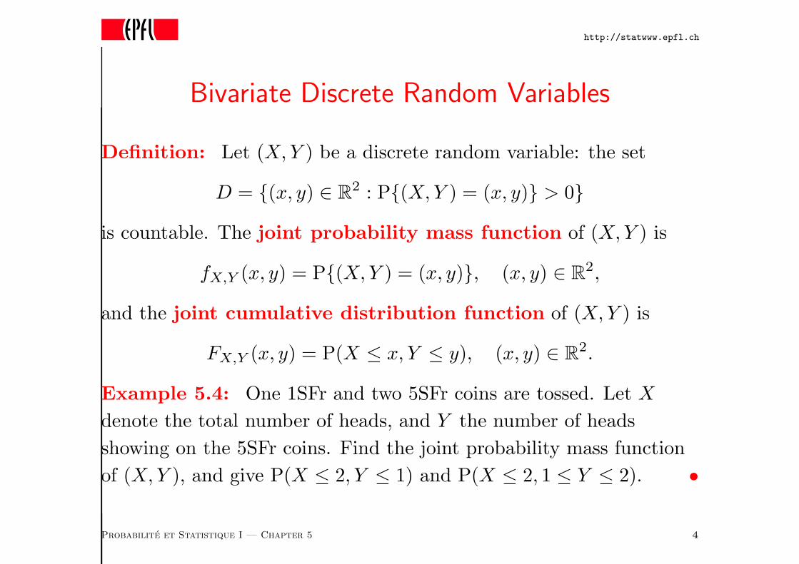
Definition: Let (X, Y ) be a discrete random variable: the set

D = (x, y) ∈ R2 : P(X, Y ) = (x, y) > 0

is countable. The joint probability mass function of (X, Y ) is

fX,Y (x, y) = P(X, Y ) = (x, y), (x, y) ∈ R2,

and the joint cumulative distribution function of (X, Y ) is

FX,Y (x, y) = P(X ≤ x, Y ≤ y), (x, y) ∈ R2.

Example 5.4: One 1SFr and two 5SFr coins are tossed. Let X

denote the total number of heads, and Y the number of heads

showing on the 5SFr coins. Find the joint probability mass function

of (X, Y ), and give P(X ≤ 2, Y ≤ 1) and P(X ≤ 2, 1 ≤ Y ≤ 2). •



Bivariate Continuous Random Variables

Definition: The random variable (X, Y ) is called (jointly)

continuous if there exists a function fX,Y (x, y) such that

P(X, Y ) ∈ A =

∫ ∫

(u,v)∈A

fX,Y (u, v) dudv

for any A ⊂ R2. Then fX,Y (x, y) is called the joint probability

density function of (X, Y ). •

On setting A = (u, v) : u ≤ x, v ≤ y, we see that the joint

cumulative distribution function of (X, Y ) may be written

FX,Y (x, y) = P(X ≤ x, Y ≤ y) =

∫ x

−∞

∫ y

−∞

fX,Y (u, v) dudv, (x, y) ∈ R2,



and this implies that

fX,Y (x, y) =∂2

∂x∂yFX,Y (x, y).

Exercise : If x1 < x2 and y1 < y2, show that

P(x1 < X ≤ x2, y1 < Y ≤ y2) = F (x2, y2)−F (x1, y2)−F (x2, y1)+F (x1, y1).

Example 5.5: Find the joint cumulative distribution function and

P(X ≤ 1, Y > 2) when

fX,Y (x, y) ∝

e−3x−2y, x, y > 0,

0, otherwise.

Example 5.6: Find the joint cumulative distribution function and

P(X ≤ 1, Y > 2) when

fX,Y (x, y) ∝

e−x−y, y > x > 0,

0, otherwise.



Marginal and Conditional Distributions

Definition: The marginal probability mass/density function

for X is

fX(x) =

∑

y fX,Y (x, y), discrete case,∫ ∞

−∞fX,Y (x, y) dy, continuous case,

x ∈ R.

The conditional probability mass/density function for Y given

X is

fY |X(y | x) =fX,Y (x, y)

fX(x), y ∈ R,

provided fX(x) > 0. When (X, Y ) is discrete,

fX(x) = P(X = x), fY |X(y | x) = P(Y = y | X = x).

Analogous definitions hold for fY (y), fX|Y (x | y), and for the

conditional distribution functions FX|Y (x | y), FY |X(y | x). The



definitions extend to several dimensions by letting X, Y be vectors. •

Example 5.7: Find the conditional and marginal probability mass

functions in Example 5.4. •

Exercise : Recompute Examples 5.4, 5.7 with three 1SFr and two

5SFr coins. •

Example 5.8: The number of eggs laid by a beetle has a Poisson

distribution with mean λ. Each egg hatches independently with

probability p. Find the distribution of the total number of eggs that

hatch. Given that x eggs have hatched, what is the distribution of

the number of eggs that were laid? •

Example 5.9: Find the conditional and marginal density functions

in Example 5.6. •



Multivariate Random Variables

Definition: Let X1, . . . , Xn be random variables defined on the

same probability space. Their joint cumulative distribution function

is

FX1,...,Xn(x1, . . . , xn) = P(X1 ≤ x1, . . . , Xn ≤ xn)

and their joint probability mass/density function is

fX1,...,Xn(x1, . . . , xn) =

P(X1 = x1, . . . , Xn = xn), discrete case,∂nFX1,...,Xn (x1,...,xn)

∂x1···∂xn, continuous case.

Marginal and conditional density and distribution functions are

defined analogously to the bivariate case, by replacing (X, Y ) with

X = X1, Y = (X2, . . . , Xn).



All the subsequent discussion can be generalised to n variables in an

obvious way, but as the notation becomes heavy we mostly stick to

the bivariate case.

Example 5.10: n students vote for the three candidates for

president of their union. Let X1, X2, X3 be the corresponding

numbers of votes, and suppose that all n students vote independently

with probabilities p1 = 0.45, p2 = 0.4, and p3 = 0.15. Show that

fX1,X2,X3(x1, x2, x3) =n!

x1!x2!x3!px11 px2

2 px33 ,

where

x1, x2, x3 ∈ 0, . . . , n, x1 + x2 + x3 = n.

Find the marginal distribution of X3, and the conditional

distribution of X1 given X3 = m. •



5.2 Independent Random Variables

Definition: Two random variables X , Y defined on the same

probability space are independent if for any subsets A,B ⊂ R,

P(X ∈ A, Y ∈ B) = P(X ∈ A)P(Y ∈ B).

This implies that the events EA = X ∈ A and EB = Y ∈ B are

independent for any sets A,B ⊂ R.

Setting A = (−∞, x] and B = (−∞, y], we have in particular

FX,Y (x, y) = P(X ≤ x, Y ≤ y)

= P(X ≤ x) P(Y ≤ y)

= FX(x)FY (y), −∞ < x, y < ∞.



This implies the equivalent condition

fX,Y (x, y) = fX(x)fY (y), −∞ < x, y < ∞,

which will be our criterion of independence.

Note: X, Y are independent if and only if this holds for all x, y ∈ R:

it is a condition on the functions fX,Y (x, y), fX(x), fY (y).

Note: If X , Y are independent, then for any x for which fX(x) > 0,

fY |X(y | x) =fX,Y (x, y)

fX(x)=

fX(x)fY (y)

fX(x)= fY (y), y ∈ R.

Thus knowledge of the value taken by X does not affect the density

of Y : this an obvious meaning of independence. By symmetry we

have also that fX|Y (x | y) = fX(x) for any y for which fY (y) > 0.

Note: If X and Y are not independent, we say they are dependent.



Example 5.11: Are (X, Y ) independent in Example 5.4? •



Example 5.14: If the density of (X, Y ) is uniform on the disk

(x, y) : x2 + y2 ≤ a,

then (a) without computing the density, say if they are independent;

(b) find the conditional density of Y given X . •

Exercise : Let ρ be a constant in the range −1 < ρ < 1. When are

the variables with joint density

fX,Y (x, y) =1

2π(1 − ρ2)1/2exp

−x2 − 2ρxy + y2

2(1 − ρ2)

, −∞ < x, y < ∞,

independent? What are then the densities of X and Y ? •



Random Sample

Definition: A random sample of size n from a distribution F

with density f is a set of n independent random variables all with

distribution F . We then write X1, . . . , Xniid∼ F or X1, . . . , Xn

iid∼ f .

The joint probability density of X1, . . . , Xniid∼ f is

fX1,...,Xn(x1, . . . , xn) =

n∏

j=1

fX(xj).

Example 5.15: If X1, X2iid∼ exp(λ), give their joint density. •

Exercise : Write down the joint density of Z1, Z2, Z3iid∼ N(0, 1),

and show that it depends only on R = (Z21 + Z2

2 + Z23 )1/2. •



5.3 Joint and Conditional Moments

Definition: Let X, Y be random variables with probability density

function fX,Y (x, y). Then the expectation of g(X, Y ) is

Eg(X, Y ) =

∑

x,y g(x, y)fX,Y (x, y), discrete case,∫∫

g(x, y)fX,Y (x, y) dxdy, continuous case,

provided E|g(X, Y )| < ∞ (so that Eg(X, Y ) has a unique value).

In particular we define joint moments and joint central moments

E(XrY s), E [X − E(X)rY − E(Y )

s] , r, s ∈ N.

The most important of these is the covariance of X and Y ,

cov(X, Y ) = E [X − E(X) Y − E(Y )] = E(XY ) − E(X)E(Y ).



Properties of Covariance

Theorem : Let X, Y, Z be random variables and a, b, c, d scalar

constants. Covariance satisfies:

cov(X, X) = var(X);

cov(a, X) = 0;

cov(X, Y ) = cov(Y, X), (symmetry);

cov(a + bX + cY, Z) = b cov(X, Z) + c cov(Y, Z), (bilinearity);

cov(a + bX, c + dY ) = bd cov(X, Y );

var(a + bX + cY ) = b2 var(X) + 2bc cov(X, Y ) + c2 var(Y );

cov(X, Y )2 ≤ var(X)var(Y ), (Cauchy–Schwarz inequality).

Use the definition of covariance to prove these. For the last, note that

var(X + aY ) is a quadratic function of a with at most one real root.



Independence and Covariance

If X and Y are independent and g(X), h(Y ) are functions whose

expectations exist, then (in the continuous case)

Eg(X)h(Y ) =

∫ ∫

g(x)h(y)fX,Y (x, y) dxdy

=

∫ ∫

g(x)h(y)fX(x)fY (y) dxdy

=

∫

g(x)fX(x) dx

∫

h(y)fY (y) dy

= Eg(X)Eh(Y ).

Setting g(X) = X − E(X) and h(Y ) = Y − E(Y ), we see that if X

and Y are independent, then

cov(X, Y ) = E [X − E(X) Y − E(Y )] = E X − E(X) E Y − E(Y ) = 0.



Independent Variables

Note: In general it is not true that cov(X, Y ) = 0 implies

independence of X and Y .

Exercise : Let X ∼ N(0, 1) and set Y = X2 − 1. What is the

conditional distribution of Y given X = x? Are they dependent?

Show that E(Xr) = 0 for any odd r. Deduce that cov(X, Y ) = 0. •

Example 5.16: Let Z1, Z2, Z3 be independent exponential variables

with parameters λ1, λ2, λ3. Let X = Z1 + Z2 and Y = Z1 + Z3. Find

cov(X, Y ) and cov(2 + 3X, 4Y ). •

Example 5.17: Let X1 ∼ N(µ1, σ21) and X2 ∼ N(µ2, σ

22) be

independent. Find the moment-generating functions of X1 and of

X1 + X2. What is the distribution of X1 + X2? •



Linear Combinations of Random Variables

Let X1, . . . , Xn be random variables and a, b1, . . . , bn constants. Then

the properties of expectation E(·) and of covariance cov(·, ·) imply

E(a + b1X1 + · · · + bbXn) = a +n

∑

j=1

bjE(Xj),

var(a + b1X1 + · · · + bbXn) =n

∑

j=1

b2jvar(Xj) +

∑

j 6=k

bjbk cov(Xj , Xk).

If X1, . . . , Xn are independent, then cov(Xj , Xk) = 0, j 6= k, and so

var(a + b1X1 + · · · + bbXn) =n

∑

j=1

b2jvar(Xj).

Example 5.18: If X1, X2 are independent variables with means 1, 2,

and variances 3, 4, find the mean and variance of 5X1 + 6X2 − 16. •



Correlation

Covariance is a poor measure of dependence between two quantities,

because it depends on their units of measurement.

Definition: The correlation of X , Y is defined as

corr(X, Y ) =cov(X, Y )

var(X)var(Y )1/2

.

Note: This measures linear dependence between X and Y . If

corr(X, Y ) = ±1 then constants a, b, c exist such that aX + bY = c

with probability one: X and Y are then perfectly linearly dependent.

If independent, they are uncorrelated: corr(X, Y ) = 0.

Note: In all cases −1 ≤ corr(X, Y ) ≤ 1.

Note: Mapping (X, Y ) 7→ (a + bX, c + dY ) changes corr(X, Y ) to

sign(bd)corr(X, Y ): at most the sign of the correlation changes.



Example 5.19: Find corr(X, Y ) in Example 5.16. •

Exercise : Let Z1, Z2, Z3 be independent Poisson variables with

common mean λ. Let X = Z1 + 2Z2 and Y = 2Z1 + Z3. Find

cov(X, Y ) and corr(X, Y ). •



Multivariate Normal Distribution

Definition: Let µ = (µ1, . . . , µn)T ∈ Rn, and let Ω be a n × n

positive definite matrix with elements ωjk. Then the vector random

variable X = (X1, . . . , Xn)T with probability density

f(x) =1

(2π)p/2|Ω|1/2exp

− 12 (x − µ)TΩ−1(x − µ)

, x ∈ Rn,

is said to have the multivariate normal distribution with mean

vector µ and covariance matrix Ω; we write X ∼ Nn(µ, Ω). This

implies that

E(Xj) = µj , cov(Xj , Xk) = ωjk.

If cov(Xj , Xk) = 0, then the variables Xj , Xk are independent.

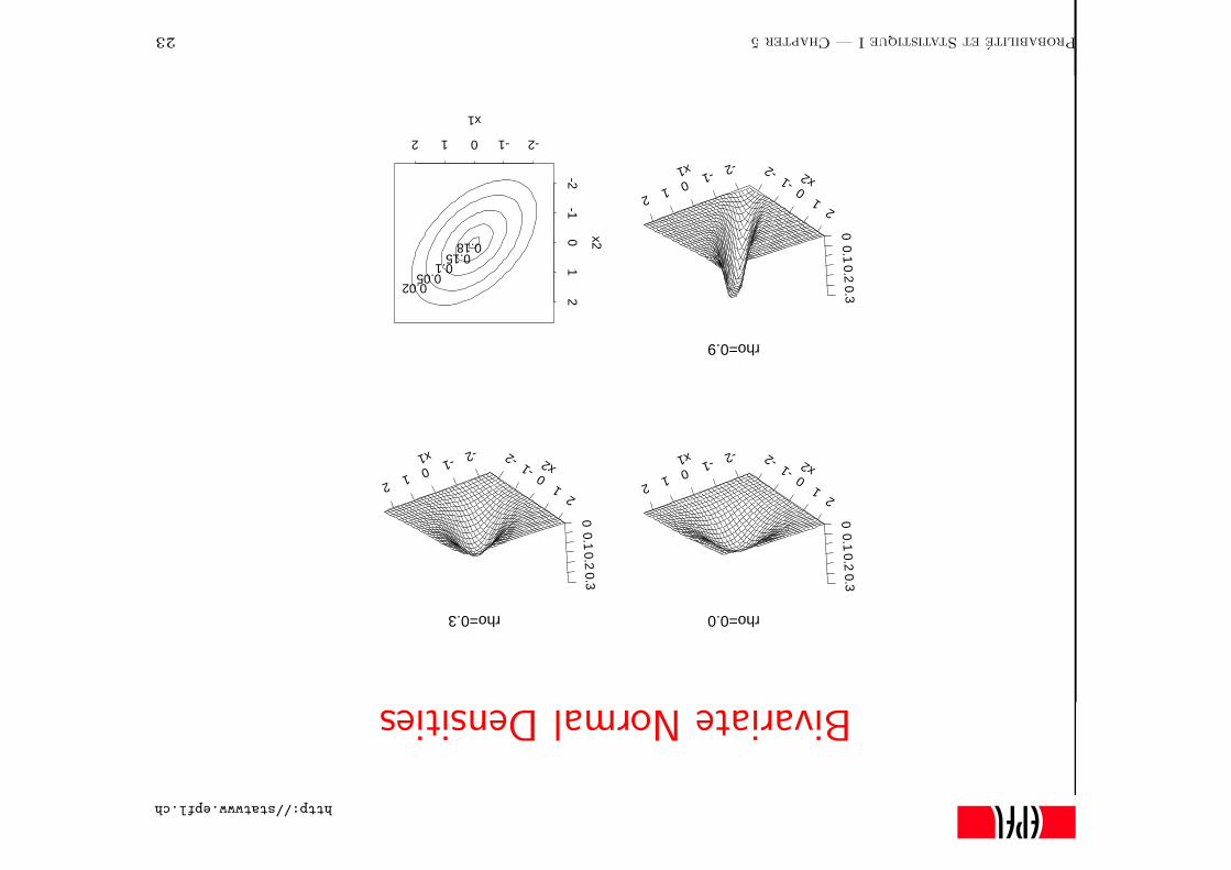
Here are plots with n = 2, zero mean (µ1 = µ2 = 0), unit variance

(ω11 = ω22 = 1), and correlation ρ = ω12/(ω11ω22)1/2.



BivariateNormalDensities

-2-1 012

x1 -2-1

01

2

x2 0

0.10.2

0.3

rho=0.0

-2-1 012

x1 -2-1

01

2

x2

00.1

0.20.3

rho=0.3

-2-1 012

x1 -2-1

01

2

x2

00.1

0.20.3

rho=0.9

x1

x2

-2-1012

-2-1

01

2

0.10.05

0.150.18

0.02

ProbabiliteetStatistiqueI—Chapter523


Conditional Expectation

Definition: Let g(X, Y ) be a function of a random variable (X, Y ).

Its conditional expectation given X = x is

Eg(X, Y ) | X = x =

∑

y g(x, y)fY |X(y | x), discrete case,∫ ∞

−∞g(x, y)fY |X(y | x) dy, continuous case,

provided fX(x) > 0 and provided E|g(X, Y )| | X = x < ∞. Notice

that this is a function of x.

Example 5.20: Find E(Y | X = x) and E(X4Y | X = x) in

Example 5.5. •

Exercise : In Example 5.7, find the expected number of eggs

hatching when n eggs have been laid. Find also the expected number

of eggs that were laid, given that m eggs have hatched. •



Iterated Expectation

In some cases it is easier to compute Eg(X, Y ) in stages. Here is

how.

Theorem (Iterated expectation): If the required expectations

exist, then

Eg(X, Y ) = EX [Eg(X, Y ) | X = x] ,

varg(X, Y ) = EX [varg(X, Y ) | X = x] + varX [Eg(X, Y ) | X = x] .

where EX and varX denote expectation and variance over the

distribution of X . •



Example 5.21: n = 200 people pass a street musician on a given

day, and each independently decides to give him money with

probability p = 0.05. The sums of money given are independent, with

means µ = 2$ and variances σ2 = 1$2. What are the mean and

variance of the money he receives? •

Exercise : A student takes a test with n = 6 questions and overall

pass mark 80. The marks for the different questions are independent.

He knows that there is a probability p = 0.1 that he will be unable to

start a question, but that if he can start then his mark for it will

have density

f(x) =

x/200, 0 ≤ x ≤ 20,

0, otherwise.

(a) What is the probability that he scores zero? (b) What are the

mean and variance of his total marks? (c) Use a normal

approximation to estimate the probability that he will pass the test.•



5.4 New Random Variables from Old

We often want to compute new random variables from old ones. Here

is how their distributions are computed.

Theorem : Let Z = g(X, Y ) be a function of random variables

(X, Y ) with joint density fX,Y (x, y). Then

FZ(z) = Pg(X, Y ) ≤ z =

∑

(x,y)∈AzfX,Y (x, y), discrete case,

∫∫

AzfX,Y (x, y) dxdy, continuous case,

where Az = (x, y) : g(x, y) ≤ z.

Example 5.22: If X, Yiid∼ exp(λ), find the distributions of X + Y

and of Y − X . •

Example 5.23: Let X1 and X2 be the results when two fair dice

are rolled independently. Find the distribution of X1 + X2. •



Tranformations of Joint Continuous Densities

Theorem : Let (X1, X2) be jointly continuous random variables,

and let Y1 = g1(X1, X2) and Y2 = g2(X1, X2), where:

(a) the simultaneous equations y1 = g1(x1, x2), y2 = g2(x1, x2) can be

solved for all (y1, y2), giving solutions x1 = h1(y1, y2), x2 = h2(y1, y2);

and

(b) g1 and g2 are continuously differentiable with Jacobian

J(x1, x2) =

∣

∣

∣

∣

∂g1

∂x1

∂g1

∂x2

∂g2

∂x1

∂g2

∂x2

∣

∣

∣

∣

which is positive whenever fX1,X2(x1, x2) > 0.

Then

fY1,Y2(y1, y2) = fX1,X2(x1, x2) |J(x1, x2)|−1

∣

∣

x1=h1(y1,y2),x2=h2(y1,y2).



Example 5.24: Find the joint density of Y1 = X1 + X2 and

Y2 = X1 − X2 when X1, X2iid∼ N(0, 1). •

Example 5.25: Find the joint density of X1 + X2 and

X1/(X1 + X2) when X1, X2iid∼ exp(λ). •

Example 5.26: If X1, X2iid∼ N(0, 1), find the density of X2/X1. •

Exercise : If the density of (X1, X2) is uniform on the unit disk

(x1, x2) : x21 + x2

2 ≤ 1, then find the density of X21 + X2

2 .

(Hint: use polar coordinates.) •



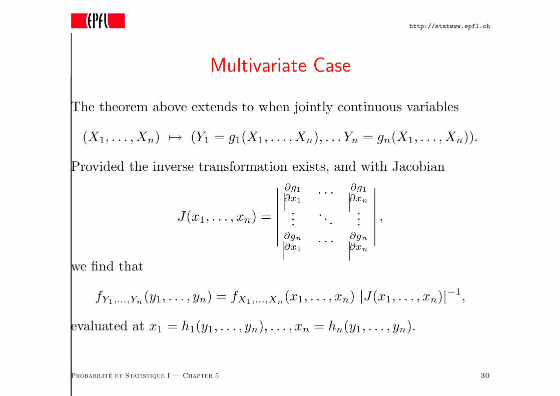
Multivariate Case

The theorem above extends to when jointly continuous variables

(X1, . . . , Xn) 7→ (Y1 = g1(X1, . . . , Xn), . . . Yn = gn(X1, . . . , Xn)).

Provided the inverse transformation exists, and with Jacobian

J(x1, . . . , xn) =

∣

∣

∣

∣

∣

∣

∣

∂g1

∂x1· · · ∂g1

∂xn

.... . .

...∂gn

∂x1· · · ∂gn

∂xn

∣

∣

∣

∣

∣

∣

∣

,

we find that

fY1,...,Yn(y1, . . . , yn) = fX1,...,Xn

(x1, . . . , xn) |J(x1, . . . , xn)|−1,

evaluated at x1 = h1(y1, . . . , yn), . . . , xn = hn(y1, . . . , yn).



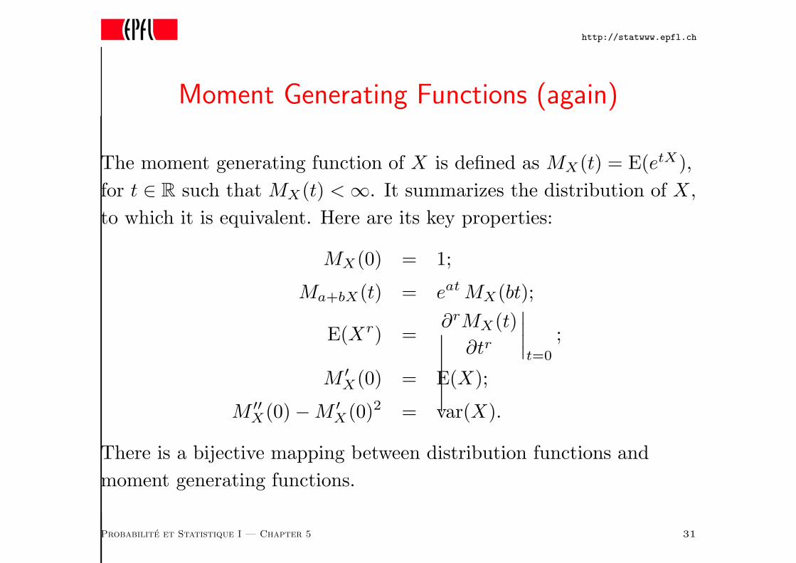
Moment Generating Functions (again)

The moment generating function of X is defined as MX(t) = E(etX),

for t ∈ R such that MX(t) < ∞. It summarizes the distribution of X ,

to which it is equivalent. Here are its key properties:

MX(0) = 1;

Ma+bX(t) = eat MX(bt);

E(Xr) =∂rMX(t)

∂tr

∣

∣

∣

∣

t=0

;

M ′X(0) = E(X);

M ′′X(0) − M ′

X(0)2 = var(X).

There is a bijective mapping between distribution functions and

moment generating functions.



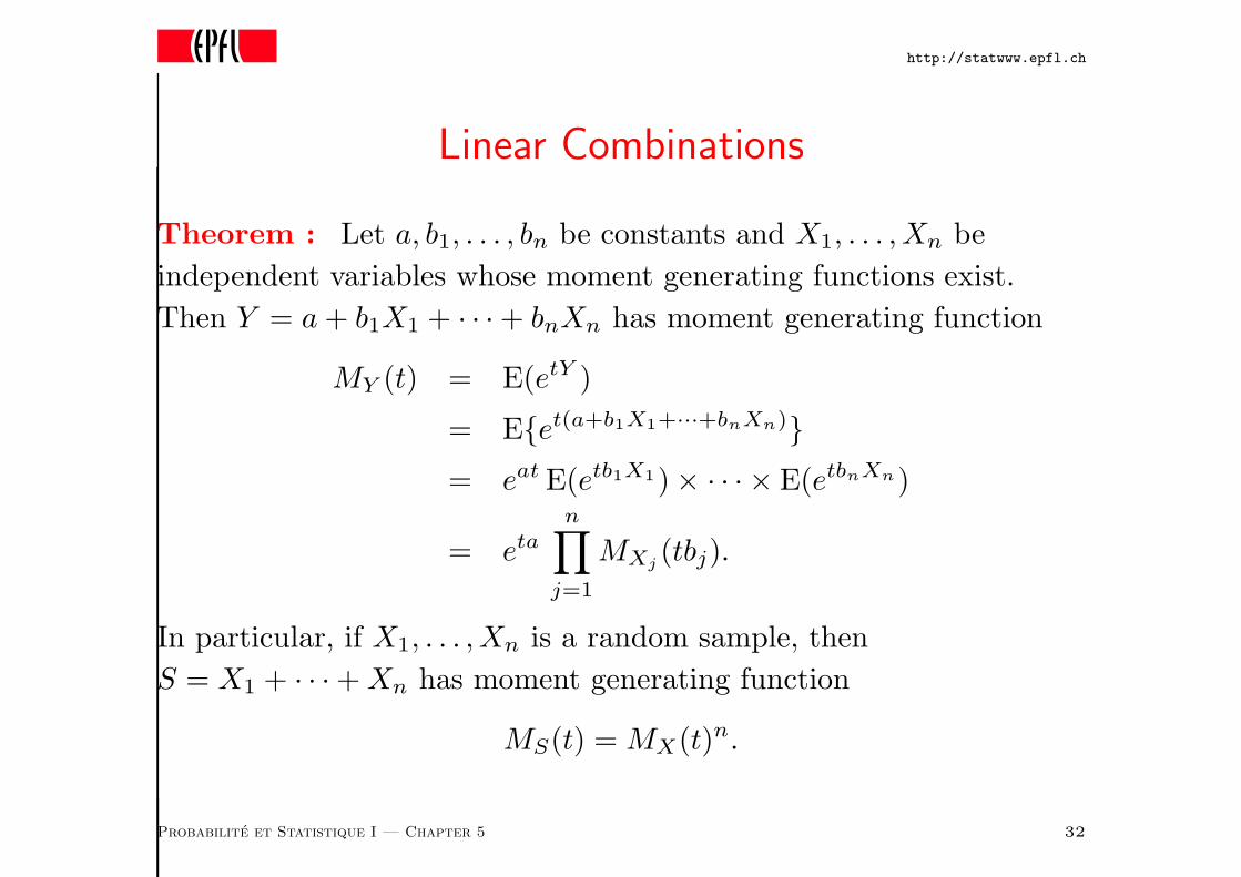
Linear Combinations

Theorem : Let a, b1, . . . , bn be constants and X1, . . . , Xn be

independent variables whose moment generating functions exist.

Then Y = a + b1X1 + · · · + bnXn has moment generating function

MY (t) = E(etY )

= Eet(a+b1X1+···+bnXn)

= eat E(etb1X1) × · · · × E(etbnXn)

= etan

∏

j=1

MXj(tbj).

In particular, if X1, . . . , Xn is a random sample, then

S = X1 + · · · + Xn has moment generating function

MS(t) = MX(t)n.



Use of Moment Generating Functions

Example 5.27: If Z ∼ N(0, 1), show that MZ(t) = et2/2. Deduce

that X = µ + σZ has MX(t) = etµ+t2σ2/2. •

Example 5.28: Suppose X1, . . . , Xn are independent, and

Xj ∼ N(µjσ2j ). Show that

Y = a+b1X1+· · ·+bnXn ∼ N(a+b1µ1+· · ·+bnµn, b21σ

21+· · ·+b2

nσ2n) :

a linear combination of normal variables is normal. •

Example 5.29: If X1, . . . , Xniid∼ exp(λ), show that

S = X1 + · · · + Xn has a gamma distribution. •

Example 5.30: If X1, X2iid∼ exp(λ), show that W = X1 −X2 has a

Laplace distribution. •



5.5 Order Statistics

Definition: The order statistics of random variables X1, . . . , Xn

are the ordered values

X(1) ≤ X(2) ≤ · · · ≤ X(n−1) ≤ X(n).

If the X1, . . . , Xn are continuous, then equality is impossible and

X(1) < X(2) < · · · < X(n−1) < X(n).

Definition: The sample minimum is X(1).

Definition: The sample maximum is X(n).

Definition: The sample median of X1, . . . , Xn is X(m+1) if

n = 2m + 1 is odd, and 12 (X(m) + X(m+1)) if n = 2m is even. The

sample median measures the location of the centre of the data.



Example 5.31: If x1 = 6, x2 = 3, x3 = 4, the order statistics are

x(1) = 3, x(2) = 4, x(3) = 6. The sample minimum, median, and

maximum are 3, 4, and 6 respectively. •

Theorem : Let X1, . . . , Xn be a random sample from a continuous

distribution with density f and distribution function F . Then

P(X(n) ≤ x) = F (x)n;

P(X(1) ≤ x) = 1 − 1 − F (x)n;

fX(r)(x) =

n!

(r − 1)!(n − r)!F (x)r−1f(x)1 − F (x)n−r, r = 1, . . . , n.

Example 5.32: Let X1, X2, X3iid∼ exp(λ). Find the marginal

densities of X(1), X(2), and X(3). •



Example 5.33: A student takes a test with 5 questions, the marks

for which are independent with density

f(x) =

x/200, 0 ≤ x ≤ 20,

0, otherwise.

Give the probability that his lowest mark is less than 5, and find the

expected values of his highest and median marks. •

Exercise : If X1, . . . , Xniid∼ F is a continuous random sample, show

that P(X(1) > x, X(n) ≤ y) = F (y) − F (x)n. Use the fact that

P(X(n) ≤ y) = P(X(1) > x, X(n) ≤ y) + P(X(1) ≤ x, X(n) ≤ y)

to show that the joint density of X(1), X(n) is

fX(1),X(n)(x, y) = n(n − 1)f(x)f(y)F (y) − F (x)n−2, x < y.

Hence give the joint density of the maximum and minimum in

Example 5.32. •


5. several random variablesstat...5.several random variables 5.1: deﬁnitions. joint density and...

Documents