582631 5 credits introduction to machine learning
TRANSCRIPT
582631 — 5 credits
Introduction to Machine Learning
Lecturer: Jyrki KivinenAssistants: Johannes Verwijnen and Amin Sorkhei
Department of Computer ScienceUniversity of Helsinki
earlier material created by Patrik Hoyer and others
27 October–11 December 2015
1 ,
Introduction
I What is machine learning? Motivation & examples
I Definition
I Relation to other fields
I Examples
I Course outline and related courses
I Practical details of the course
I Lectures
I Exercises
I Exam
I Grading
2 ,

What is machine learning?
I Definition:
machine = computer, computer program (in this course)
learning = improving performance on a given task, basedon experience / examples
I In other words
I instead of the programmer writing explicit rules for how tosolve a given problem, the programmer instructs the computerhow to learn from examples
I in many cases the computer program can even become betterat the task than the programmer is!
3 ,
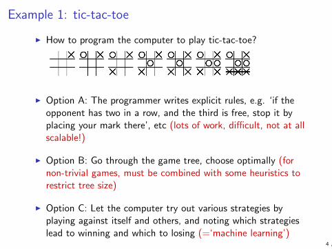
Example 1: tic-tac-toe
I How to program the computer to play tic-tac-toe?
I Option A: The programmer writes explicit rules, e.g. ‘if theopponent has two in a row, and the third is free, stop it byplacing your mark there’, etc (lots of work, difficult, not at allscalable!)
I Option B: Go through the game tree, choose optimally (fornon-trivial games, must be combined with some heuristics torestrict tree size)
I Option C: Let the computer try out various strategies byplaying against itself and others, and noting which strategieslead to winning and which to losing (=‘machine learning’)
4 ,
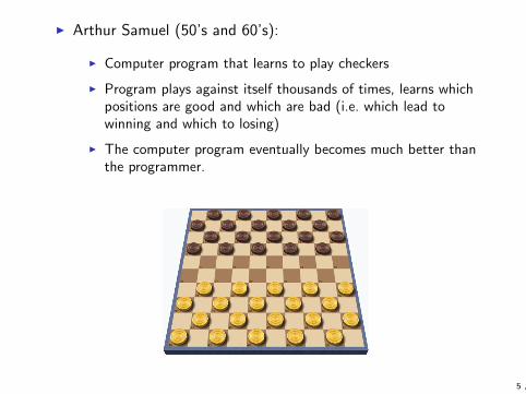
I Arthur Samuel (50’s and 60’s):
I Computer program that learns to play checkers
I Program plays against itself thousands of times, learns whichpositions are good and which are bad (i.e. which lead towinning and which to losing)
I The computer program eventually becomes much better thanthe programmer.
5 ,
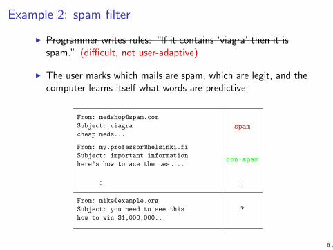
Example 2: spam filter
I Programmer writes rules: “If it contains ‘viagra’ then it isspam.” (difficult, not user-adaptive)
I The user marks which mails are spam, which are legit, and thecomputer learns itself what words are predictive
Example 2: spam filter
� X is the set of all possible emails (strings)
� Y is the set { spam, non-spam }
From: [email protected]
Subject: viagra
cheap meds...spam
From: [email protected]
Subject: important information
here’s how to ace the test...non-spam
......
From: [email protected]
Subject: you need to see this
how to win $1,000,000...?
6 ,6 ,
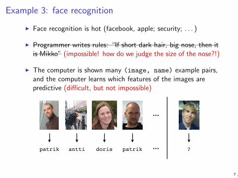
Example 3: face recognition
I Face recognition is hot (facebook, apple; security; . . . )
I Programmer writes rules: “If short dark hair, big nose, then itis Mikko” (impossible! how do we judge the size of the nose?!)
I The computer is shown many (image, name) example pairs,and the computer learns which features of the images arepredictive (difficult, but not impossible)
patrik antti doris patrik
...
... ?
7 ,
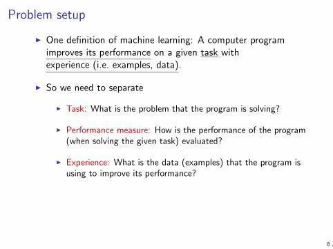
Problem setup
I One definition of machine learning: A computer programimproves its performance on a given task withexperience (i.e. examples, data).
I So we need to separate
I Task: What is the problem that the program is solving?
I Performance measure: How is the performance of the program(when solving the given task) evaluated?
I Experience: What is the data (examples) that the program isusing to improve its performance?
8 ,
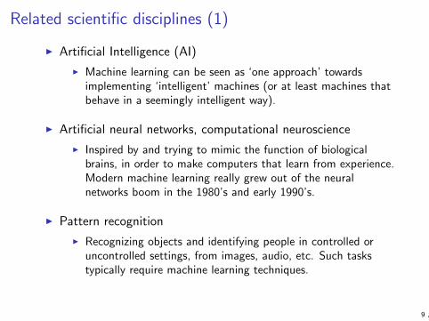
Related scientific disciplines (1)
I Artificial Intelligence (AI)
I Machine learning can be seen as ‘one approach’ towardsimplementing ‘intelligent’ machines (or at least machines thatbehave in a seemingly intelligent way).
I Artificial neural networks, computational neuroscience
I Inspired by and trying to mimic the function of biologicalbrains, in order to make computers that learn from experience.Modern machine learning really grew out of the neuralnetworks boom in the 1980’s and early 1990’s.
I Pattern recognition
I Recognizing objects and identifying people in controlled oruncontrolled settings, from images, audio, etc. Such taskstypically require machine learning techniques.
9 ,
Availability of data
I These days it is very easy toI collect data (sensors are cheap, much information digital)I store data (hard drives are big and cheap)I transmit data (essentially free on the internet).
I The result? Everybody is collecting large quantities of data.I Businesses: shops (market-basket data), search engines (web
pages and user queries), financial sector (stocks, bonds,currencies etc), manufacturing (sensors of all kinds), socialnetworking sites (facebook, twitter), anybody with a webserver (hits, user activity)
I Science: genomes sequenced, gene expression data,experiments in high-energy physics, images of remote galaxies,global ecosystem monitoring data, drug research anddevelopment, public health data
I But how to benefit from it? Analysis is becoming key!
10 ,

Big Data
I one definition: data of a very large size, typically to the extentthat its manipulation and management present significantlogistical challenges (Oxford English Dictionary)
I 3V: volume, velocity, and variety (Doug Laney, 2001)
I a database may be able to handle a lot of data, but you can’timplement a machine learning algorithm as an SQL query
I on this course we do not consider technical issues relating toextremely large data sets
I basic principles of machine learning still apply, but manyalgorithms may be difficult to implement efficiently
11 ,

Related scientific disciplines (2)
I Data miningI Trying to identify interesting and useful associations and
patterns in huge datasets
I Focus on scalable algorithms
I Example: shopping basket analysis
I StatisticsI historically, introductory courses on statistics tend to focus on
hypothesis testing and some other basic problemsI however there’s a lot more to statistics than hypothesis testingI there is a lot of interaction between research in machine
learning, data mining and statistics
12 ,

Example 4
I Prediction of search queries
I The programmer provides a standard dictionary (words andexpressions change!)
I Previous search queries are used as examples!
13 ,

Example 5
I Ranking search results:
I Various criteria forranking results
I What do users click onafter a given search?Search engines canlearn what users arelooking for bycollecting queries andthe resulting clicks.
14 ,

Example 6
I Detecting credit card fraud
I Credit card companies typically end uppaying for fraud (stolen cards, stolen cardnumbers)
I Useful to try to detect fraud, for instancelarge transactions
I Important to be adaptive to the behaviorsof customers, i.e. learn from existing datahow users normally behave, and try todetect ‘unusual’ transactions
15 ,

Example 7
I Self-driving cars:
I Sensors (radars,cameras) superior tohumans
I How to make thecomputer reactappropriately to thesensor data?
16 ,

Example 8
I Character recognition:
I Automatically sortingmail (handwrittencharacters)
I Digitizing old booksand newspapers intoeasily searchableformat (printedcharacters)
17 ,

Example 9
I Recommendation systems(‘collaborative filtering’):
I Amazon: ”Customerswho bought X alsobought Y ”...
I Netflix: ”Based onyour movie ratings, youmight enjoy...”
Challenge: One milliondollars ($1,000,000)prize money recentlyawarded!
4 5 5 1 2
3 4 3
1 4 1 5 1
? 4 1 ?2 1 1 5
1 1 4 5
4 5 5
2 3 3
Fargo
Seven
Leon
Aliens
Avatar
Bill
Jack
Linda
John
Lucy
18 ,

Example 10
I Machine translation:
I Traditional approach: Dictionary and explicit grammar
I More recently, statistical machine translation based onexample data is increasingly being used
19 ,

Example 11
I Online store websiteoptimization:
I What items to present,what layout?
I What colors to use?
I Can significantly affectsales volume
I Experiment, andanalyze the results!(lots of decisions onhow exactly toexperiment and how toensure meaningfulresults)
20 ,

Example 12
I Mining chat and discussion forums
I Breaking news
I Detecting outbreaks of infectious disease
I Tracking consumer sentiment about companies / products
21 ,

Example 13
I Real-time sales andinventory management
I Picking up quickly onnew trends (what’s hotat the moment?)
I Deciding on what toproduce or order
22 ,

Example 14
I Prediction of friends in Facebook, or prediction of who you’dlike to follow on Twitter.
23 ,

What about privacy?
I Users are surprisingly willing to sacrifice privacy to obtainuseful services and benefits
I Regardless of what position you take on this issue, it isimportant to know what can and what cannot be done withvarious types information (i.e. what the dangers are)
I ‘Privacy-preserving data mining’
I What type of statistics/data can be released without exposingsensitive personal information? (e.g. government statistics)
I Developing data mining algorithms that limit exposure of userdata (e.g. ‘Collaborative filtering with privacy’, Canny 2002)
24 ,

Course outline
I Introduction
I Ingredients of machine learning
I task
I models
I data
I Supervised learning
I classification
I regression
I evaluation and model selection
I Unsupervised learning
I clustering
I matrix decompositions
25 ,
Related courses
I Various continuation courses at CS (spring 2015):
I Probabilistic Models (period III, plus optional project)
I Project in Practical Machine Learning (period III)
I Advanced Machine Learning (period IV)
I Data Mining (period III, plus optional project)
I Big Data Frameworks (period IV)
I A number of other specialized courses at CS department
I A number of courses at maths+stats
I Lots of courses at Aalto as well
26 ,

Practical details (1)
I Lectures:
I 27 October (today) – 11 December
I Tuesdays and Fridays at 10:15–12:00 in Exactum C222
I Lecturer: Jyrki Kivinen(Exactum B229a, [email protected])
I Language: English
I Based on parts of the course textbook (next slide)
I (previous instances of this course used a different textbook)
27 ,

Practical details (2)
I Textbook:
I author: Peter Flach
I title: Machine Learning. The Art andScience of Algorithms that Make Sense ofData.
I publisher: Cambridge University Press(2012, first edition)
I author’s web page:https://www.cs.bris.ac.uk
/~flach/mlbook/
I we’ll cover Chapters 1–3, main ideas inChapters 4–6, and quite a lot of Chapters7–9
28 ,

Practical details (3)
I Lecture material
I this set of slides (by JK, partly using previous years’ coursematerials) is intended for use as part of the actual lectures,together with the blackboard etc.
I the textbook author has a full set of much more polished slidesavailable on his web page
I however the lectures will cover some issues in more detail thanthe textbook
I in particular some additional detail is needed for homeworkproblems
I both the lectures and the assigned parts of the textbook arerequired material for the exam
29 ,

Practical details (4)
I Exercises:
I course assistants: Johannes Verwijnen and Amin SorkheiI Learning by doing:
I mathematical exercises (pen-and-paper)I computer exercises (support given in Python)
I Problem set handed out every Friday, focusing on topics fromthat week’s lectures
I Deadline for handing in your solutions is next Friday at 23:59.
I In the exercise session on the day before deadline (Thu14:15–16:00), you can discuss the problems with the assistantand with other students.
I Attending exercise sessions is completely voluntary.
I Language of exercise sessions: English
I Exercise points make up 40% of your total grade, must get atleast half the points to be eligible for the course exam.
I Details will appear on the course web page.
30 ,

Practical details (5)
I Exercises this week:
I No regular exercise session this week.
I Instead: instruction on Python and its libraries that are usefulon this course
I Tuesday 27 October (today!) at 12:15–16:00 in B221
I Voluntary, no points awarded. Recommended for everyone notpreviously familiar with Python.
I Assistant will be available between 12:15–16:00; you don’thave to be there at 12 and may leave before 16
I You don’t have to use Python for the course work if you prefersome other language. Ask the course assistants about whichalternatives are acceptable.
31 ,

Practical details (6)
I Course exam:
I 16 December at 9:00 (double-check a few days before theexam)
I Constitutes 60% of your course grade
I Must get a minimum of half the points of the exam to passthe course
I Pen-and-paper problems, similar style as in exercises (also‘essay’ or ‘explain’ problems)
I (Note: To be eligible to take a ‘separate exam’ you need to first
complete some programming assignments. These will be available
on the course web page a bit later. However since you are here at
the lecture, this probably does not concern you.)
I You may answer exam problems also in Finnish or Swedish.
32 ,

Practical details (7)
I Grading:
I Exercises: (typically: 3 pen-and-paper and 1 programmingproblem per week)
I Programming problem graded to 0–15 pointsI Pen-and-paper problems graded to 0–3 pointsI First week’s Python exercises: Voluntary, no pointsI Late homework policy will be explained on course web page
I Exam: (4–5 problems)I Pen-and-paper: 0–6 points/problem (tentative)
I Rescaling done so that 40% of total points come fromexercises, 60% from exam
I Half of all total points required for lowest grade, close tomaximum total points for highest grade
I Note: Must get at least half the points of the exam, and mustget at least half the points available from the exercises
33 ,
Practical details (8)
I Prerequisites:
I Mathematics: Basics of probability theory and statistics, linearalgebra and real analysis
I Computer science: Basics of programming (but no previousfamiliarity with Python necessary)
I Prerequisites quiz!
I For you to get a sense of how well you know the prerequisites
I For me to get a sense of how well you (in aggregate!) knowthe prerequisites. Fully anonymous!
34 ,

Practical details (9)
I Course material:
I Webpage (public information about the course):http://www.cs.helsinki.fi/en/courses/582631/2015/s/k/1
I Sign up in Ilmo (department registration system)
I Help?
I Ask the assistants/lecturer at exercises/lectures
I Contact assistants/lecturer separately
35 ,

Questions?
36 ,
Ingredients of machine learning
37 ,

Ingredients of machine learning: Outline
I We take a first look into some basic components of a machinelearning scenario, such as task, data, features, model.
I We will soon get back to all this on a more technical level.
I Read Prologue and Chapter 1 from textbook.
38 ,
Summary of the setting
I Task is what an end user actually wants to do.
I Model is a (hopefully good) solution to the task.
I Data consists of objects in the domain the user is interestedin, with perhaps some additional information attached.
I Machine learning algorithm produces a model based on data.
I Features are how we represent the objects in the domain.
39 ,
Task
I Task is an actual data processing problem some end userneeds to solve.
I Examples were given in lecture 1 (image recognition, frauddetection, ranking web pages, collaborative filtering, . . . )
I Typically, a task involves getting some input and thenproducing the appropriate output.
I For example, in hand-written digit recognition, the input is apixel matrix representing an image of a digit, and the outputis one of the labels ’0’, . . . , ’9’.
I Machine learning is a way to find a solution (basically, analgorithm) for this data processing problem when it’s toocomplicated or poorly understood for a programmer (or anapplication specialist) to figure it out.
40 ,

Supervised learning
Many common tasks belong to the area of supervised learningwhere we neeed to produce some target value (often called label):
I binary classification: divide inputs into two categoriesI Example: classify e-mail messages into spam and non-spam
I multiclass classification: more than two categoriesI Example: classify an image of a digit into one of the classes
’0’, . . . , ’9’
I multilabel classification: multiple classes, of which more thanone may match simultaneously
I Example: classify news stories based on their topics
I regression: output is a real-valuedI Example: predict the value of a house based on its size,
location etc.
41 ,
Unsupervised learning
In unsupervised learning, there is no specific target value ofinterest.Examples of unsupervised learning tasks:
I clustering: partition the given set of data into clusters so thatelements that belong to same cluster are similar (in terms ofsome given similarity measure)
I association rules: for example, given shopping cart contents ofdifferent customers, find product combinations that are oftenbought together
I dimensionality reduction: if the data is high-dimensional (eachdata point is described by a large number of variables), findan alternative lower-dimensional representation that retains asmuch of the structure as possible
42 ,
Semisupervised learning
Unsupervised learning can be used as pre-processing to helpsupervised learning
I for example, classifying images
I Internet has as many non-classified images as we could everwant
I less easy to label the data (assign the correct class to eachimage)
I solution: use the unlabelled images to find a low-dimensionalrepresentation, then use a smaller set of labelled images tosolve the hopefully easier lower-dimensional classificationproblem
43 ,
Predictive vs. descriptive model
I Predictive model: our ultimate goal is to predict some targetvariable
I Descriptive model: no specific target variable, we want tounderstand the data
I distinction between supervised vs. unsupervised learning iswhether the target values are available to the learningalgorithm
I Examples:I predictive and supervised: classification, regression
I descriptive and unsupervised: clustering
I descriptive and supervised: find subgroups that behavedifferently with respect to the target variable
I predictive and unsupervised: clustering, with the clusters thenused to assign classes
44 ,

Evaluating performance on a task
I When we apply machine learning techniques, we haveavailable some training data which we use to come up with agood model
I However what really counts is generalisation: performance onfuture unseen data that was not in the training set; this iscalled
I Overfitting is the mistake of building a too complicated modelusing too little training data
I results look very good on training data
I however performance on unseen data is bad
I to get an unbiased estimate on performance on unseen data,one can withhold part of the training data and use it as testset when learning is finished (but not before!)
45 ,

Latent variables
Latent (or hidden) variables describe underlying structure of thedata that is not immediately obvious in the original input variables.
I Example: we have N persons and M movies, and an N ×Mmatrix of scores where sij is the score given by person i tomovie j .
I We might try to represent this using K latent variables (let’scall them genres, but remember that they are not given aspart of the data):
I pik is 1 is person i likes genre k , and 0 otherwise
I qkj is 1 is movie j belongs to genre k , and 0 otherwise
I wk is the importance of belonging to genre k
46 ,

Latent variables (2)
I if for some K � min {M,N } we can find (pik), (qkj) and(wk) such that
K∑
k=1
wkpikqkj ≈ sij for all i and j
then we have found some interesting structure.
I In the new representation we have K (N + M + 1) parameters,as opposed to the original NM.
47 ,

Features
I Features define the vocabulary we use to describe the objectsin the domain of interest (the “original inputs” of the task).
I Finding the right features is extremely important.
I However it’s often also highly dependent on the application.
I Basic approaches to finding good features includeI ask someone who understands the domain
I use some standard set of features
I analyse the data
I On this course we see some examples of often used features,but mostly we don’t consider where the features come from.
48 ,
Features (2)
I Examples of how features can be formed:I take the Fourier transformation of an audio signal
I find edges, corners and other basic elements from an image
I scaling numerical inputs to have similar ranges
I representing a document as bag of words (what words appearin the document, and how many times each)
I bag of words can be extended to consider pairs, triples etc. ofwords
I the kernel trick is a way of using certain types of features incertain types of learning algorithms in a computationallyefficient manner
49 ,

Similarity and dissimilarity
I Notions of similarity and dissimilarity between objects areimportant in machine learning
I clustering tries to group similar objects together
I many classification algorithms are based on the idea thatsimilar objects tend to belong to same class
I etc.
I We cover the topic here a bit more thoroughly that thetextbook since this is one of the topics for first homework
I You should also read textbook Section 8.1 on distancemeasures
50 ,

I Examples: think about suitable similarity measures forI handwritten letters
I segments of DNA
I text documents
“Parliament overwhelmingly approved amendments to the Firearms Act on Wednesday. The new law requires physicians to inform authorities of individuals they consider unfit to own guns. It also increases the age for handgun ownership from 18 to 20.”
“Parliament's Committee for Constitutional Law says that persons applying for handgun licences should not be required to join a gun club in the future. Government is proposing that handgun users be part of a gun association for at least two years.”
“The cabinet on Wednesday will be looking at a controversial package of proposed changes in the curriculum in the nation's comprehensive schools. The most divisive issue is expected to be the question of expanded language teaching.”
ACCTGTCGATCCTGTGTCGATTGC
51 ,

I Similarity: s
I Numerical measure of the degree to which two objects are alike
I Higher for objects that are alike
I Typically between 0 (no similarity) and 1 (completely similar)
I Dissimilarity: d
I Numerical measure of the degree to which two objects aredifferent
I Higher for objects that are different
I Typically between 0 (no difference) and ∞ (completelydifferent)
I Transformations
I Converting from one to the other
I Use similarity or dissimilarity measures?
I Method-specific
52 ,

Similarity for bit vectors
I Objects are often represented by d-bit vectors for some d
I This may arise naturally, or because we represent objects usingd features which are all binary valued
I Consider now two n-bit vectors
I Let fab denote the number of positions where first vector hasa and second has b
I Thus f00 + f01 + f10 + f11 = d
53 ,

Similarity for bit vectors (2)
I Hamming distance (dissimilarity)
H = f01 + f10 (1)
I Simple matching coefficient
SMC =f11 + f00
f11 + f00 + f01 + f10(2)
I Jaccard coefficient
J =f11
f11 + f01 + f10(3)
54 ,

Dissimilarity in Rd
I We start by defining the p-norm (or Lp norm) ford-dimensional real vector z = (z1, . . . , zd) ∈ Rd as
‖z‖p =
(d∑
i=1
|zi |p)1/p
I For p ≥ 1 this actually satisfies the definition of a norm (seesome book on real analysis)
I We then define Minkowski distance between x and y as
Disp(x, y) = ‖x− y‖p
I p = 2: Euclidean distance
I p = 1: “Manhattan” or ”city block” distance
55 ,
Dissimilarity in Rd (2)
I For p ≥ 1, Minkowski distance is a metric:I Dis(x, x) = 0
I Dis(x, y) > 0 if x 6= y
I Dis(x, y) = Dis(y, x)
I triangle inequality:
Dis(x, z) ≤ Dis(x, y) + Dis(y, z)
I For p < 1 the triangle inequality does not hold
56 ,

Dissimilarity in Rd (3)
I Considering the limit p →∞ leads to defining also
‖z‖∞ = max { |zi | | i = 1, . . . , d }
I We also define 0-norm as the number of non-zero components
‖z‖0 =d∑
i=1
I [zi 6= 0]
where I [φ] = 1 if φ is true and I [φ] = 0 otherwise.
57 ,

Chess problem
Reti 1921 White to play and draw
58 ,
L∞ distance in chess
I Textbook makes some points about distance measures inchess (pp. 232–233)
I Perhaps the most interesting point is that movements of aKing follow L∞ distance
I moves diagonally as fast as horizontally and vertically
I This leads to some counterintuitive results (see famousproblem on previous slide)
59 ,
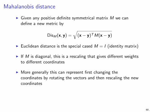
Mahalanobis distance
I Given any positive definite symmetrical matrix M we candefine a new metric by
DisM(x, y) =√
(x− y)TM(x− y)
I Euclidean distance is the special cased M = I (identity matrix)
I If M is diagonal, this is a rescaling that gives different weightsto different coordinates
I More generally this can represent first changing thecoordinates by rotating the vectors and then rescaling the newcoordinates
60 ,

Similarity in Rd
I Cosine similarity (ranges from -1 to 1)
cos(x, y) =x · y
‖x‖2 ‖y‖2
where x · y =∑d
i=1 xiyi
I Pearson’s correlation coefficient (ranges from -1 to 1)
r =
∑di=1(xi − x)(yi − y)√∑d
i=1(xi − x)2
√∑di=1(yi − y)2
where x = 1d
∑di=1 xi , and y similarly
61 ,

Models: the output of machine learning
I We have a preliminary look into what kinds of models arecommonly considered
I We cover this topic a bit more lightly than the textbook(Section 1.2) since this will be covered in much more detailwhen we get to actual machine learning algorithm
I The various classifications of models should not be taken toorigidly. The purpose is just to see some different ideas we canapply when thinking about models
62 ,

Geometric models
I Instances are the objects in our domain that we wish to, say,classify.
I Instance space is the set of all conceivable instances ourmodel should be able to handle
I Geometric models treat instances as vectors in Rd and usenotions such as
I angle between vectors
I distance, length of a vector
I dot product
63 ,
Nearest neighbour classifier
I Nearest-neighbour classifier is a simple geometric model basedon distances:
I store all the training data
I to classify a new data point, find the closest one in thetraining set and use its class
I More generally, k-nearest-neighbour classifier (for someinteger k) finds k nearest points in the training set and usesthe majority class (ties are broken arbitrarily)
I Different notions of distance can be used, but Euclidean is themost obvious
64 ,

Linear classifier
I Linear classifier is a simple non-local geometric model
I Any weight vector w ∈ Rd defines a classifier
f (x) =
{1 if w · x > 0−1 otherwise
I We divide instances to classes along the hyperplane{ x | w · x = 0 }
I If we want to consider hyperplanes that do not pass throughorigin, we may replace the condition by w · x + b > 0 where bis another parameter (to be determined by the learningalgorithm, like w)
65 ,

Basic linear classifier
I We learn a simple binary classifier from training data{ (xi , yi ) | i = 1, . . . , n } where xi ∈ Rd and y ∈ {−1, 1 }
I Let P = { xi | yi = 1 } be the set of positive examples withcentre point
p =1
|P|∑
x∈Px
I Similarly let n be the centre of negative examples
I Now w = p− n is the vector from n to p, and m = (p + n)/2is the point in the middle
66 ,

Basic linear classifier (2)
I The basic binary classifier is given by
f (x) =
{1 if w · x > w ·m−1 otherwise
I It splits the instance space into positive and negative partthrough the mid-point between p and n
I We can also interpret the basic linear classifier as adistance-based model that classifies x depending on which ofthe prototypes p and n is closer
67 ,

Probabilistic models
I Probabilistic approach to machine learning is in particularused in generative learning
I For example in supervised learning, the task is to predict sometarget values Y given observed values X
I However in practice we don’t usually think that X somehowcauses Y
I E.g. in medicine, we need to predict disease based onsymptoms, but causally it’s the disease that causes thesymptoms
68 ,

Probabilistic models (2)
I Generative model is a joint distribution P(X ,Y ) for both Xand Y
I Given P(X ,Y ), we can predict Y based on X :
P(Y | X ) =P(X ,Y )
P(X )
whereP(X ) =
∑
Y
P(X ,Y )
69 ,

Probabilistic models (3)
I In contrast to generative model, a discriminative model justtries to find out what separates, say, X values associated withY = 1 from X values associated with Y = −1
I In terms of probabilities, discriminative learning can be seen asmodelling just P(Y | X ) and ignoring P(X )
I Avoids solving a more difficult problem than we really need
I However throws away some information
70 ,
Logical models
I Typical logical models are based on rules
if condition then label
where the condition contains feature values and possiblylogical connectives
I Decision trees are a popular logical model class that cantextually be represented as a nested if-then-else structure
I Logical models are often more easily understood by humansI But large decision trees can be very confusing
71 ,

Grouping and grading
I Linear models are typical grading modelsI w · x gets arbitrary real values
I for any x1 and x2 with w · x1 < w · x2 we can find t such thatw · x1 < t < w · x2
I Decision tree models are typical grouping modelsI Usually a large number of instances end up in the same leaf of
the tree
I If two instances are in the same leaf, they always receive thesame label
I Grading models allow for more fine grained separation ofinstances than grouping models
72 ,

Binary classification and related tasks
73 ,
Binary classification: Outline
I We consider more closely the binary classification task
I In particular, we consider performance measures
I Ranking is closely related to binary classificationI Many learning algorithms actually solve a ranking problem
I Ranking can then be converted into binary classifier
I We consider the notion of Bayes optimality in a bit moredetail than the textbook
I Read Sections 2.1 and 2.2 from the textbook; we deferSection 2.3 until we have more to say about learningprobabilistic models
74 ,
Basic setting
I Instance space X : inputs of the model
I Output space Y: outputs of the model
I In supervised learning, the input to the learning algorithmtypically consists of examples (x , y) ∈ X × Y that somehowexhibit the desired behaviour of the model
I We may also have a separate label space L 6= Y, so thatexamples are from X × L
I for example, labels are classes, outputs class probabilities
75 ,

Supervised learning tasks
I classification: L = Y = C where C = {C1, . . . ,Ck } is the setof classes
I case |C| = 2 is called binary classification
I multilabel classification: L = Y = 2C where 2A denotes thepower set of A (the set of all subsets of A)
I scoring and ranking: L = C and Y = R|C|
I probability prediction: L = C and Y = [0, 1]|C|
I regression: L = Y = R
76 ,
Supervised learning
I Input of the learning algorithm is a training set Tr ⊂ X × Lconsisting of pairs (x , l) where l ∈ C
I Ideally the training set consists of pairs (x , l(x)) for someunknown function l : X → L which we would like to know(sometimes called target function)
I Output of the learning algorithm is a function l : X → L(often called hypothesis) that hopefully is a goodapproximation of l
I In practice the training set does not contain perfect examplesof a target function
I instance and label get corrupted by noise
I there may not be sufficient information to fully determine thelabel
77 ,

Supervised learning (2)
I To evaluate the performance of the hypothesis l , we need atest set Te ⊂ X × L
I sometimes both Tr and Te are given
I more often you are just given some data and need to split itinto Tr and Te yourself
I Ideally for all (x , l) ∈ Te we have l = l(x)
I We shall look into more realistic performance measures verysoon
I In all cases it is important not to use the test data duringtraining (i.e. until you have fully decided on the output l)
I we are interested in performance on new unseen data
I evaluating on same data that was used for learning givesover-optimistic results and leads to too complicatedhypotheses (overfitting)
78 ,

Supervised learning (3)
I Usually the instances are given in terms of a finite number offeatures
I If we have d features, and feature i takes values in domain Fi ,we have X = F1 × · · · × Fd .
I We don’t here consider where the features come from
I Notice that although any feature values can usually beencoded as real numbers, this may lead to problems if donecarelessly
I suppose we encode feature Country so that Germany is 17,Finland is 18 and France is 19
I a geometric learning algorithm might interpret that
Finland =Germany + France
2
79 ,

Assessing classifier performance
I Notation:I c(x) is the true label of instance x
I c(x) is the label predicted for x by the classifier we areassessing
I In binary classification labels are in {−1,+1 }I Te+ is the set of all positive examples:
Te+ = { x | (x ,+1) ∈ Te }= { x ∈ Te | c(x) = +1 }
I Te− is the set of all negative examples
I Pos =∣∣Te+
∣∣ and Neg =∣∣Te−
∣∣
80 ,

Contingency table
I Also known as confusion matrix
I Generally an |L| × |Y| matrix where cell (l , y) has the numberof instances x such that c(x) = l and c(x) = y
I We consider binary classification and hence 2× 2 matrices
predict + predict − total
actual + TP FN Posactual − FP TN Neg
total TP + FP TN + FN |Te|
I P/N: prediction is + or −I T/F: prediction is correct (“true”) or incorrect (“false”)
I row and column sums are called marginals
81 ,

Performance metrics for binary classification
I Accuracy = (TP + TN)/(TP + TN + FP + FN)
I Error rate = 1− Accuracy
I True positive rate (‘sensitivity’) = TP/(TP + FN)
I True negative rate (‘specificity’) = TN/(TN + FP)
I False positive rate = FP/(TN + FP)
I False negative rate = FN/(TP + FN)
I Recall = TP/(TP + FN)
I Precision = TP/(TP + FP)
82 ,

Performance metrics (2)
I If we want to summarise classifier performance in one number(instead of the whole contingency table), accurary is mostcommonly used
I However sometimes considering just accuracy is not enoughI unbalanced class distribution (e.g. information retrieval)
I different cost for false positive and false negative (e.g. spamfiltering, medical diagnostics)
I We will soon consider more closely the idea of assigningdifferent costs to different mistakes
83 ,
Coverage plot
I Coverage plot is a way to visualise the performance of abinary classifier on a data set
I Horizontal axis ranges from 0 to Neg
I Vertical axis ranges from 0 to Pos
I An algorithm is represented by the point (FP,TP)I up and left is good
I down and right is bad
84 ,

Coverage plot (2)
I To compare two algorithms A and B on the same data set, weplot their corresponding points (FPA,TPA) and (FPB ,TPB)
I If A is to up and left of B, we say that A dominates BI In this case FPA < FPB and TPA > TPB
I Since Pos = TP + FN, we also have FNA < FNB
I Hence A is more accurate than B on both classes
I If A is to up and right of B, there is no clear comparisonI A makes fewer false negatives but more false positives than B
I In particular if A and B are on the same line with 45 degreeslope, they have same accuracy
I TPA − TPB = FPA − FPB so FPA + FNA = FPB + FNB
85 ,

Coverage plot (3)
I Coverage plot in range [0,Neg]× [0,Pos] are calledunnormalised
I It is also common to scale the coordinates to range in [0, 1]
I We then plot an algorithm at point (fpr, tpr)
I If Pos 6= Neg, the slopes in the figure changeI Lines with 45 degree slope now connect algorithms with same
average recall defined as (tpr + tnr)/2
I Normalised coverage plots are known as ROC plots (fromReceiver Operating Characteristic in signal processing)
86 ,
Cost function for classification
I Consider classification with k classes c1, . . . , ck
I Let L(ci , cj) be the cost or loss incurred when we predictc(x) = ci but the correct label is c(x) = cj
I ideally these are actual costs related to the application
I in practice we may not have any real costs available
I The default choice is 0-1 loss which just counts the number ofmistakes:
L01(ci , cj) =
{0 if ci = cj1 otherwise
I Generally we may have an arbitrary k × k cost matrix whereelement (j , i) contains L(ci , cj)
I Usually we can assume that diagonal entries are 0
87 ,

Total cost of classification
I Given a confusion matrix and a cost matrix, we can calculatethe total cost of the classifications by elementwisemultiplication
I Example:
predict+ −
actual+ 27 3− 6 38
Confusion matrix
predict+ −
actual+ 0 30− 1 0
Cost matrix
I Here the total cost is 27 · 0 + 3 · 30 + 6 · 1 + 38 · 0 = 96
88 ,
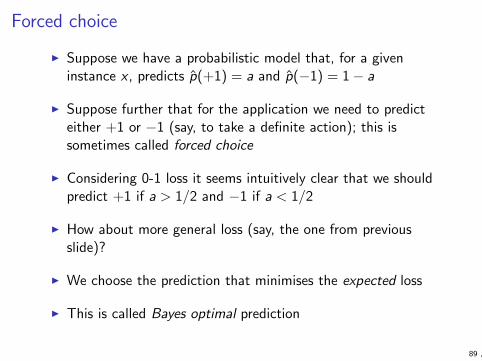
Forced choice
I Suppose we have a probabilistic model that, for a giveninstance x , predicts p(+1) = a and p(−1) = 1− a
I Suppose further that for the application we need to predicteither +1 or −1 (say, to take a definite action); this issometimes called forced choice
I Considering 0-1 loss it seems intuitively clear that we shouldpredict +1 if a > 1/2 and −1 if a < 1/2
I How about more general loss (say, the one from previousslide)?
I We choose the prediction that minimises the expected loss
I This is called Bayes optimal prediction
89 ,
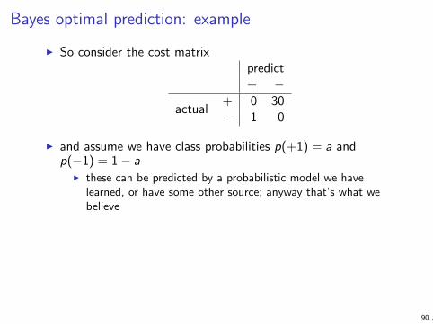
Bayes optimal prediction: example
I So consider the cost matrixpredict+ −
actual+ 0 30− 1 0
I and assume we have class probabilities p(+1) = a andp(−1) = 1− a
I these can be predicted by a probabilistic model we havelearned, or have some other source; anyway that’s what webelieve
90 ,

Bayes optimal prediction: example (2)
I If we predict +1, we have probability a of loss 0, andprobability 1− a of loss 1, so the expected loss isa · 0 + (1− a) · 1 = 1− a
I If we predict −1, we have probability a of loss 30, andprobability 1− a of loss 0, so the expected loss isa · 30 + (1− a) · 0 = 30a
I So we should predict +1 if 1− a < 30a, which holds ifa < 1/31
91 ,

Bayes optimality in general
I Bayes optimality applies to decision making also outsidemachine learning
I Consider the following scenario:I we make an observation x
I we have a set of actions Y we can take
I for each action y ∈ Y and outcome l ∈ L there is a costL(y , l) ∈ R
I We have a conditional probability P(l | x) over outcomes givenx
I We want to choose action y that minimises the expected loss
∑
l∈LL(y , l)P(l | x)
92 ,

Bayesian classifier
I We now develop the idea of Bayes optimality a bit further forclassifiers
I Suppose we have a probabilistic model P(x , y)
I Probabilistic learning algorithms often learn P(x , y) byseparately learning P(y) and P(x | y), from which we getP(x , y) = P(x | y)P(y)
I From Bayes rule we get
P(y | x) =P(x , y)
P(x)=
P(y)P(x | y)
P(x)
I Note that the denominator is a constant (so when maximizingthe left-hand-side with respect to y it can safely be ignored)
I We can also write it out as P(x) =∑
y P(x , y)93 ,

Bayesian classifier (2)
I Suppose we are now given probabilities P(x , y) and costsL(y , y ′) for x ∈ X and y , y ′ ∈ C
I We consider the expected cost of a classifier c : X → C, oftencalled risk:
Risk(c) =∑
(x ,y)∈X×C
P(x , y)L(y , c(x))
I We want to find a minimum risk classifier
c∗ = arg minc
Risk(c)
I For historical reasons, the minimum cost classifier c∗ is calledBayes optimal, and its associated risk Risk(c∗) the Bayeserror or risk
94 ,
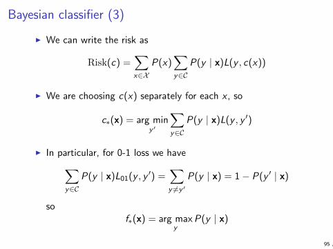
Bayesian classifier (3)
I We can write the risk as
Risk(c) =∑
x∈XP(x)
∑
y∈CP(y | x)L(y , c(x))
I We are choosing c(x) separately for each x , so
c∗(x) = arg miny ′
∑
y∈CP(y | x)L(y , y ′)
I In particular, for 0-1 loss we have
∑
y∈CP(y | x)L01(y , y ′) =
∑
y 6=y ′
P(y | x) = 1− P(y ′ | x)
sof∗(x) = arg max
yP(y | x)
95 ,

Cost functions for probabilistic classification
I Output of the model is now a probability distribution P(·)over C
I Labels are still individual classes c ∈ C
I Typical cost functions includeI logarithmic cost
L(P, c) = − log P(c)
I linear costL(P, c) = 1− P(c)
96 ,
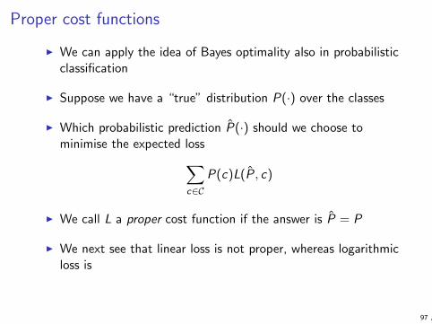
Proper cost functions
I We can apply the idea of Bayes optimality also in probabilisticclassification
I Suppose we have a “true” distribution P(·) over the classes
I Which probabilistic prediction P(·) should we choose tominimise the expected loss
∑
c∈CP(c)L(P, c)
I We call L a proper cost function if the answer is P = P
I We next see that linear loss is not proper, whereas logarithmicloss is
97 ,

Linear cost is not proper
I Say the true distribution is P(c = −1) = 1/4,P(c = +1) = 3/4
I Set the predicted distribution to P(c = −1) = b,P(c = +1) = 1− b
I The expected cost is
Ec [L(P, c)] = Ec [1− P(c)]
=1
4(1− b) +
3
4(1− (1− b))
=1
4+
1
2b
I This is minimized for b = 0, not the true probability b = 1/4.
98 ,

Logarithmic cost is proper
I We show this for the binary case
I Say the true distribution is P(c = −1) = a andP(c = +1) = 1− a for an arbitrary 0 ≤ a ≤ 1.
I Set the predicted distribution to P(c = −1) = b,P(c = +1) = 1− b
I The expected logarithmic loss is
Ec [L(P, c)] = −a log b − (1− a) log(1− b)
I We claim this is minimised for b = a
99 ,
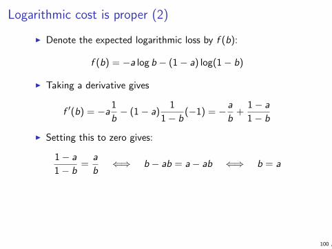
Logarithmic cost is proper (2)
I Denote the expected logarithmic loss by f (b):
f (b) = −a log b − (1− a) log(1− b)
I Taking a derivative gives
f ′(b) = −a1
b− (1− a)
1
1− b(−1) = −a
b+
1− a
1− b
I Setting this to zero gives:
1− a
1− b=
a
b⇐⇒ b − ab = a− ab ⇐⇒ b = a
100 ,

Logarithmic cost is proper (3)
I Take the second derivative:
f ′′(b) =a
b2− 1− a
(1− b)2(−1) =
a
b2+
1− a
(1− b)2> 0
I Hence b = a is the unique minimum
I So the logarithmic cost is proper according to the definition.
101 ,

Scoring
I A scoring classifier with k classes outputs for instance x avector of k real-valued scores
s(x) = (s1(x), . . . , sk(x))
I Large value si (x) means x is likely to belong to class Ci
I In binary classification we usually just consider a single score,with large s(x) denoting class +1 and small s(x) denotingclass −1
I For example a linear model gives a scoring functions(x) = w · x− t
I We get a binary classifier naturally as c(x) = sign(s(x))
102 ,

Loss functions for binary scoring
I Consider a score-based classifier c(x) = sign(s(x))
I Given a label c(x) ∈ {−1,+1 } we have c(x) = c(x) ifc(x)s(x) > 0
I The quantity z(x) = c(x)s(x) is called (signed, unnormalised)margin
I We usually consider the “non-prediction” s(x) = 0 as mistake
I We get the 0-1 loss L01(s(x), c(x)) = I [c(x)s(x) ≤ 0]
I Summing over Te gives the usual error rate (with minorreservation concerning how the case s(x) = 0 is handled)
I Another common loss function is the hinge loss Lh(z) = 0 ifz ≥ 1 and Lh(z) = 1− z if z < 1
103 ,

Classification, scoring and ranking
I Given a scoring function s, we can create a ranking of a set ofinstances x by ordering them according to s(x)
I Consider for example document retrievalI c(x) = +1 denotes that document x is relevant for a given
query, and c(x) = −1 irrelevant
I we obtain a scoring function s(·)I we offer documents to user in order of decreasing s(x)
104 ,
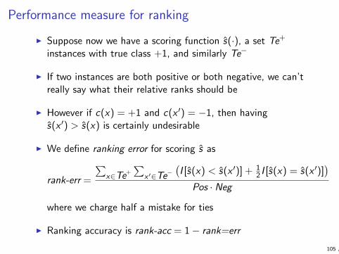
Performance measure for ranking
I Suppose now we have a scoring function s(·), a set Te+
instances with true class +1, and similarly Te−
I If two instances are both positive or both negative, we can’treally say what their relative ranks should be
I However if c(x) = +1 and c(x ′) = −1, then havings(x ′) > s(x) is certainly undesirable
I We define ranking error for scoring s as
rank-err =
∑x∈Te+
∑x ′∈Te−
(I [s(x) < s(x ′)] + 1
2 I [s(x) = s(x ′)])
Pos · Neg
where we charge half a mistake for ties
I Ranking accuracy is rank-acc = 1− rank=err
105 ,
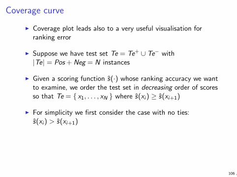
Coverage curve
I Coverage plot leads also to a very useful visualisation forranking error
I Suppose we have test set Te = Te+ ∪ Te− with|Te| = Pos + Neg = N instances
I Given a scoring function s(·) whose ranking accuracy we wantto examine, we order the test set in decreasing order of scoresso that Te = { x1, . . . , xN } where s(xi ) ≥ s(xi+1)
I For simplicity we first consider the case with no ties:s(xi ) > s(xi+1)
106 ,

Coverage curve (2)
I For k = 1, . . . ,N − 1, pick any tk such thats(xk) > tk > s(xk+1)
I Further, pick t0 > s(x1) and tN < s(xN)
I Consider now the N + 1 classifiers ck(·) where
ck(x) =
{+1 if s(x) > tk−1 otherwise
I Classifiers ck are based on same scoring but have differentthreshold for predicting +1
I We have ck(xi ) = +1 for i ≤ k and ck(xi ) = −1 for i > k
107 ,

Coverage curve (3)
I Coverage curve for scoring s(·) is now obtained by plottingthe N + 1 classifiers ck(·) into same coverage plot andconnecting the points from left to right
I c0(x) = −1 for all x , so the curve starts from (0, 0)
I cN(x) = +1 for all x , so curve ends at (Neg,Pos)
I Going from ck−1 to ck changes the classification of xk from−1 to +1, but nothing else
I if c(xk) = +1, it becomes true positive and the curve movesone step up
I if c(xk) = −1, it becomes false positive and the curve movesone step right
108 ,

Coverage curve (4)
I Coverage curve is drawn on Neg + 1 by Pos + 1 grid
I There are Pos + Neg + 1 grid points precisely on the curve, sothere are Pos · Neg points that are strictly above or strictlybelow the curve
I We will next show that the number of grid points strictlybelow the curve is
∑
x∈Te+
∑
x ′∈Te−I [s(x) > s(x ′)]
I Consequently, the number of points above the curve is
∑
x∈Te+
∑
x ′∈Te−I [s(x) < s(x ′)]
109 ,

ROC curve
I ROC curve is the same as coverage curve, except that it’sdrawn with axes scaled to [0, 1]
I This gives the correct normalisation so that area under ROCcurve (often written just as AUC) is precisely ranking accuracy
I In literature outside the textbook, ROC curves are morecommon than unnormalised coverage curves
110 ,
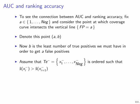
AUC and ranking accuracy
I To see the connection between AUC and ranking accuracy, fixa ∈ { 1, . . . ,Neg } and consider the point at which coveragecurve intersects the vertical line {FP = a }
I Denote this point (a, b)
I Now b is the least number of true positives we must have inorder to get a false positives
I Assume that Te− ={
x−1 , . . . , x−Neg
}is ordered such that
s(x−i ) > s(x−i+1)
111 ,

AUC and ranking accuracy (2)
I Then b is the number of points x ∈ Te+ such thats(x) > s(x−a ):
b =∑
x∈Te+
I [s(x) > s(x−a )]
I Since grid starts at 0, this is also the number of grid pointsbelow the curve in column {FB = a }
I Summing over a gives the claim
112 ,
AUC and ranking accuracy (3)
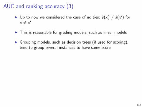
I Up to now we considered the case of no ties: s(x) 6= s(x ′) forx 6= x ′
I This is reasonable for grading models, such as linear models
I Grouping models, such as decision trees (if used for scoring),tend to group several instances to have same score
113 ,
AUC and ranking accuracy (4)
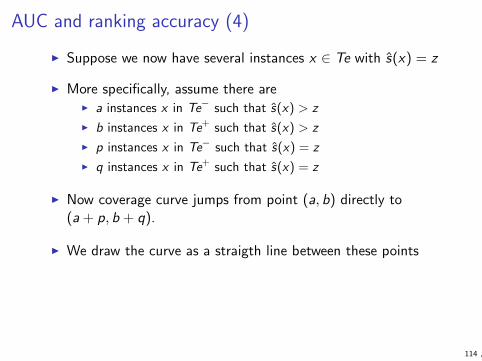
I Suppose we now have several instances x ∈ Te with s(x) = z
I More specifically, assume there areI a instances x in Te− such that s(x) > z
I b instances x in Te+ such that s(x) > z
I p instances x in Te− such that s(x) = z
I q instances x in Te+ such that s(x) = z
I Now coverage curve jumps from point (a, b) directly to(a + p, b + q).
I We draw the curve as a straigth line between these points
114 ,
AUC and ranking accuracy (5)
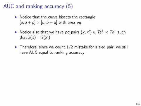
I Notice that the curve bisects the rectangle[a, a + p]× [b, b + q] with area pq
I Notice also that we have pq pairs (x , x ′) ∈ Te+ × Te− suchthat s(x) = s(x ′)
I Therefore, since we count 1/2 mistake for a tied pair, we stillhave AUC equal to ranking accuracy
115 ,

Turning ranker into classifier
I As we just saw, a ranking of N instances gives rise to N + 1different binary classifiers depending on where we set thethreshold
I Each classifier corresponds to a corner of the ROC curve
I Different points on ROC curve represent different possiblepairs (fpr, tpr)
I We now consider which one to choose
I We want to pick one as close to top left corner of the ROCplot as possible
I Proper notion of closeness depends on what precisely we wantfrom the classifier
116 ,
Turning ranker into classifier (2)
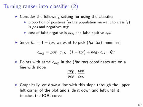
I Consider the following setting for using the classifierI proportion of positives (in the population we want to classify)
is pos and negatives neg
I cost of false negative is cFN and false positive cFP
I Since fnr = 1− tpr, we want to pick (fpr, tpr) minimize
cavg = pos · cFN · (1− tpr) + neg · cFP · fpr
I Points with same cavg in the (fpr, tpr) coordinates are on aline with slope
neg
pos· cFP
cFN
I Graphically, we draw a line with this slope through the upperleft corner of the plot and slide it down and left until ittouches the ROC curve
117 ,

Evaluating model performance
118 ,

Evaluating models: Outline
I A fundamental issue in machine learning is that we buildmodels based on training data, but really care aboutperformance on new unseen test data
I Generalisation refers to the learned model’s ability to workwell also on unseen data
I good generalisation: what we learned from training data alsoapplies to test data
I poor generalisation: what seemed to work well on training datais not so good on test data
119 ,
Goals for this chapter
I Familiarity with the basic ideas of evaluating generalisationperformance of (supervised) learning system
I Ability to explain overfitting and underfitting with examples
I Ability to explain with examples the idea of model complexityand its relation to overfitting and underfitting
I Using separate training, validation and test sets and crossvalidation in practice
120 ,

About the textbook
I Issues related to generalisation and evaluating modelperformance appear in several parts of the textbook
I overfitting in many places
I bias vs. variance in Section 3.2
I statistical learning theory in Section 4.4
I cross validation in Section 12.2
I We collect the main ideas together here before proceeding tospecific machine learning algorithms
I Some of this material is not in the textbook in this form
I We’ll skip most of Chapter 4 which introduces certain types oflogical models we’ll not be using on this course
121 ,

Why we measure performance
I After we are otherwise quite done with learning, we maymeasure the performance of the final model to assess itsusefulness in the actual application (is it good enough for realuse)
I We also measure performance of various models duringlearning to make informed choices
I what type of model to use
I how to set parameters of our learning algorithm
I most importantly for the current discussion: choosing rightmodel complexity (often called model class selection)
122 ,

How good is my classifier?
I Apply the learned classifier to the training data?
I k-Nearest Neighbor with k = 1 performs at 100% accuracy(each point is the nearest neighbor of itself, so label is correct!)
I k-Nearest Neighbor with k > 1 generally performs < 100%
I linear classifier also generally gives < 100% accuracy
I Many other classifiers (such as decision trees or rule-basedclassifiers, coming soon!) can achieve 100% accuracy as well,as long as all records x are distinct
⇒ so never use kNN with k > 1 or linear classifier?
I But... the goal of classification is to perform well on new(unseen) data. How can we test that?
123 ,

Statistical learning model
I We consider supervised learning: goal is to learn a functionf : X → Y.
I During learning, we create f based on training set{ (x1, y1), . . . , (xN , yN) } where (xi , yi ) ∈ X × Y
I Later we test f on unseen data points{ (xN+1, yN+1), . . . , (xN+M , yN+M) }
I We have a loss function L : Y × Y → R and wish to minimisethe average loss on unseen data
1
M
M∑
i=1
L(f (xN+i ), yN+i )
124 ,

Statistical learning model (2)
I Assume further that we have a fixed but unknown probabilitydistribution P over X × Y such that pairs are (xi , yi ) areindependent samples from it
I We say the data points are independent and identicallydistibuted (i.i.d.)
I We wish to minimise the generalisation error (also called truerisk) of f , which is the expected error
E(x ,y)∼P [L(f (x), y)]
where E(x ,y)∼P [·] denotes expectation when (x , y) is drawnfrom P
125 ,

Statistical learning model (3)
I If P were known, this would just be the decision-theoreticproblem of finding a Bayes-optimal prediction
I Now P is not known, where learning comes to picture
I Since also training data is drawn from P, we can use it tomake more or less accurate inferences about properties of P
126 ,
How good is my classifier (2)
I So, we can estimate the generalization error by using only partof the available data for ‘training’ and leaving the rest for‘testing’.
I under the stated assumptions the test data is now ‘new data’,so we can with this approach get unbiased estimates of thegeneralization error
I Typically (almost invariably), the performance on the test setis worse than on the training set, because the classifier haslearned some properties specific to the training set (inaddition to properties of the underlying distribution)
127 ,

I Comparing 1NN, kNN, Naive Bayes, and any other classifieron a held-out test set:
I Now all generally perform < 100%
I Not a priori clear which method is best, this is an empiricalissue (and depends on the amount of data, the structure in thedata, etc)
I Flexible classifiers may overfit the training data.
I Spam filter: Picking up on words that discriminate the twoclasses in the training set but not in the distribution
I Credit card fraud detection: Some thieves may use the card tobuy regular items; those particular items (or itemcombinations) may then be marked suspicious
I Face recognition: It happened to be darker than average whenone of the pictures was taken. Now darkness is associated withthat particular identity.
128 ,

Overfitting
I Overfitting means creating models that follow too closely thespecifics of the training data, resulting in poor performance onunseen data
I Overfitting often results from using too complex models withtoo little data
I complex models allow high accuracy but require lots of data totrain
I simple models require less training data but are incapable ofmodelling complex phenomena accurately
I Choosing the right model complexity is a difficult problem forwhich there are many methods
129 ,
What is model complexity?
I For parametric models the number of parameters is often anatural measure of complexity (e.g. linear model in ddimensions, degree k polynomial)
I Some non-parametric models also have an intuitive complexitymeasure (e.g. number of nodes in decision tree)
I There are also less obvious parameters that can be used tocontrol overfitting (e.g. kernel width, parameter k in kNN,norm of coefficient vector in linear model)
I Mathematical study of various formal notions of complexity isa vast field outside the scope of this course
I Here we’ll only discuss these notions on the level of basicintuition and simple applications
130 ,
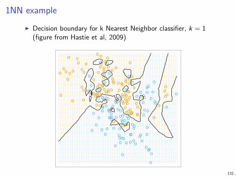
1NN example
I Decision boundary for k Nearest Neighbor classifier, k = 1(figure from Hastie et al, 2009)16 2. Overview of Supervised Learning
1-Nearest Neighbor Classifier
.. .. .. . . . . .. . . . . . .. . . . . . . . .. . . . . . . . .. . . . . . . . . . .. . . . . . . . . . . . . .. . . . . . . . . . . . . . .. . . . . . . . . . . . . . . . . .. . . . . . . . . . . . . . . . . . .. . . . . . . . . . . . . . . . . . . .. . . . . . . . . . . . . . . . . . . . .. . . . . . . . . . . . . . . . . . . . . . . . . .. . . . . . . . . . . . . . . . . . . . . . . . .. . . . . . . . . . . . . . . . . . . . . . . .. . . . . . . . . . . . . . . . . . . . . . . .. . . . . . . . . . . . . . . . . . . . . . . .. . . . . . . . . . . . . . . . . . . . . . . . . .. . . . . . . . . . . . . . . . . . . . . . . . . .. . . . . . . . . . . . . . . . . . . . . . . . . .. . . . . . . . . . . . . . . . . . . . . . . . . . .. . . . . . . . . . . . . . . . . . . . . . . . . . . .. . . . . . . . . . . . . . . . . . . . . . . . . . . . . .. . . . . . . . . . . . . . . . . . . . . . . . . . . . . . .. . . . . . . . . . . . . . . . . . . . . . . . . . . . . . . . .. . . . . . . . . . . . . . . . . . . . . . . . . . . . . . . . . .. . . . . . . . . . . . . . . . . . . . . . . . . . . . . . . . . . . . .. . . . . . . . . . . . . . . . . . . . . . . . . . . . . . . . . . . . . .. . . . . . . . . . . . . . . . . . . . . . . . . . . . . . . . . . . . . .. . . . . . . . . . . . . . . . . . . . . . . . . . . . . . . . . . . . . . . .. . . . . . . . . . . . . . . . . . . . . . . . . . . . . . . . . . . . . . . .. . . . . . . . . . . . . . . . . . . . . . . . . . . . . . . . . . . . . . . . .. . . . . . . . . . . . . . . . . . . . . . . . . . . . . . . . . . . . . . . . . .. . . . . . . . . . . . . . . . . . . . . . . . . . . . . . . . . . . . . . . . .. . . . . . . . . . . . . . . . . . . . . . . . . . . . . . . . . . . . . . . . . . . .. . . . . . . . . . . . . . . . . . . . . . . . . . . . . . . . . . . . . . .. . . . . . . . . . . . . . . . . . . . . . . . . . . . . . . . . . . . .. . . . . . . . . . . . . . . . . . . . . . . . . . . . . . . . . . . . . . . .. . . . . . . . . . . . . . . . . . . . . . . . . . . . . . . . . . . . . . . . . . .. . . . . . . . . . . . . . . . . . . . . . . . . . . . . . . . . . . . . . . . . . . . . .. . . . . . . . . . . . . . . . . . . . . . . . . . . . . . . . . . . . . . . . . . . . . . . . .. . . . . . . . . . . . . . . . . . . . . . . . . . . . . . . . . . . . . . . . . . . . . . . .. . . . . . . . . . . . . . . . . . . . . . . . . . . . . . . . . . . . . . . . . . . . . .. . . . . . . . . . . . . . . . . . . . . . . . . . . . . . . . . . . . . . . . . . . .. . . . . . . . . . . . . . . . . . . . . . . . . . . . . . . . . . . . . . . . . . .. . . . . . . . . . . . . . . . . . . . . . . . . . . . . . . . . . . . . . . . . . . .. . . . . . . . . . . . . . . . . . . . . . . . . . . . . . . . . . . . . . . . . . . . . . . .. . . . . . . . . . . . . . . . . . . . . . . . . . . . . . . . . . . . . . . . . . . . . .. . . . . . . . . . . . . . . . . . . . . . . . . . . . . . . . . . . . . . . . . . . . .. . . . . . . . . . . . . . . . . . . . . . . . . . . . . . . . . . . . . . . . . . .. . . . . . . . . . . . . . . . . . . . . . . . . . . . . . . . . . . . . . . . . . . . .. . . . . . . . . . . . . . . . . . . . . . . . . . . . . . . . . . . . . . . . . . . .. . . . . . . . . . . . . . . . . . . . . . . . . . . . . . . . . . . . . . . . . . . . .. . . . . . . . . . . . . . . . . . . . . . . . . . . . . . . . . . . . . . . . . . . . . . .. . . . . . . . . . . . . . . . . . . . . . . . . . . . . . . . . . . . . . . . . . . . . . . . .. . . . . . . . . . . . . . . . . . . . . . . . . . . . . . . . . . . . . . . . . . . . . . .. . . . . . . . . . . . . . . . . . . . . . . . . . . . . . . . . . . . . . . . . . . . . .. . . . . . . . . . . . . . . . . . . . . . . . . . . . . . . . . . . . . . . . . . . . . .. . . . . . . . . . . . . . . . . . . . . . . . . . . . . . . . . . . . . . . . . . . .. . . . . . . . . . . . . . . . . . . . . . . . . . . . . . . . . . . . . . . . . . . . . . .. . . . . . . . . . . . . . . . . . . . . . . . . . . . . . . . . . . . . . . . . . . . . . .. . . . . . . . . . . . . . . . . . . . . . . . . . . . . . . . . . . . . . . . . . . . . . . . . . .. . . . . . . . . . . . . . . . . . . . . . . . . . . . . . . . . . . . . . . . . . . . . . . . . . . . . . . . .. . . . . . . . . . . . . . . . . . . . . . . . . . . . . . . . . . . . . . . . . . . . . . . . . . . . . . . . . .. . . . . . . . . . . . . . . . . . . . . . . . . . . . . . . . . . . . . . . . . . . . . . . . . . . . . . . . . .. . . . . . . . . . . . . . . . . . . . . . . . . . . . . . . . . . . . . . . . . . . . . . . . . . . . . . . . .. . . . . . . . . . . . . . . . . . . . . . . . . . . . . . . . . . . . . . . . . . . . . . . . . . . . .. . . . . . . . . . . . . . . . . . . . . . . . . . . . . . . . . . . . . . . . . . . . . . . . . .. . . . . . . . . . . . . . . . . . . . . . . . . . . . . . . . . . . . . . . . . . . . . . . . .. . . . . . . . . . . . . . . . . . . . . . . . . . . . . . . . . . . . . . . . . . . . . . . . . .. . . . . . . . . . . . . . . . . . . . . . . . . . . . . . . . . . . . . . . . . . . . . . . . . . . . . . .. . . . . . . . . . . . . . . . . . . . . . . . . . . . . . . . . . . . . . . . . . . . . . . . . . . . . . . . . .. . . . . . . . . . . . . . . . . . . . . . . . . . . . . . . . . . . . . . . . . . . . . . . . . . . . . . . . . . .. . . . . . . . . . . . . . . . . . . . . . . . . . . . . . . . . . . . . . . . . . . . . . . . . . . . . . . . . . .. . . . . . . . . . . . . . . . . . . . . . . . . . . . . . . . . . . . . . . . . . . . . . . . . . . . . . . . . . .. . . . . . . . . . . . . . . . . . . . . . . . . . . . . . . . . . . . . . . . . . . . . . . . . . . . . . . . . . .. . . . . . . . . . . . . . . . . . . . . . . . . . . . . . . . . . . . . . . . . . . . . . . . . . . . . . . . . . . .
. . . . . . . . . . . . . . . . . . . . . . . . . . . . . . . . . . . . . . . . . . . . . . . . . . . . . . . . . . . . . . . . . . . . .. . . . . . . . . . . . . . . . . . . . . . . . . . . . . . . . . . . . . . . . . . . . . . . . . . . . . . . . . . . . . . . . . . . . .. . . . . . . . . . . . . . . . . . . . . . . . . . . . . . . . . . . . . . . . . . . . . . . . . . . . . . . . . . . . . . . . . . . . .. . . . . . . . . . . . . . . . . . . . . . . . . . . . . . . . . . . . . . . . . . . . . . . . . . . . . . . . . . . . . . . . . . . . .. . . . . . . . . . . . . . . . . . . . . . . . . . . . . . . . . . . . . . . . . . . . . . . . . . . . . . . . . . . . . . . . . . . . .. . . . . . . . . . . . . . . . . . . . . . . . . . . . . . . . . . . . . . . . . . . . . . . . . . . . . . . . . . . . . . . . . . . . .. . . . . . . . . . . . . . . . . . . . . . . . . . . . . . . . . . . . . . . . . . . . . . . . . . . . . . . . . . . . . . . . . . . . .. . . . . . . . . . . . . . . . . . . . . . . . . . . . . . . . . . . . . . . . . . . . . . . . . . . . . . . . . . . . . . . . . . . . .. . . . . . . . . . . . . . . . . . . . . . . . . . . . . . . . . . . . . . . . . . . . . . . . . . . . . . . . . . . . . . . . . . . . .. . . . . . . . . . . . . . . . . . . . . . . . . . . . . . . . . . . . . . . . . . . . . . . . . . . . . . . . . . . . . . . . . . . . .. . . . . . . . . . . . . . . . . . . . . . . . . . . . . . . . . . . . . . . . . . . . . . . . . . . . . . . . . . . . . . . . . . . . .. . . . . . . . . . . . . . . . . . . . . . . . . . . . . . . . . . . . . . . . . . . . . . . . . . . . . . . . . . . . . . . . . . . . .. . . . . . . . . . . . . . . . . . . . . . . . . . . . . . . . . . . . . . . . . . . . . . . . . . . . . . . . . . . . . . . . . . . . .. . . . . . . . . . . . . . . . . . . . . . . . . . . . . . . . . . . . . . . . . . . . . . . . . . . . . . . . . . . . . . . . . . . . .. . . . . . . . . . . . . . . . . . . . . . . . . . . . . . . . . . . . . . . . . . . . . . . . . . . . . . . . . . . . . . . . . . . . .. . . . . . . . . . . . . . . . . . . . . . . . . . . . . . . . . . . . . . . . . . . . . . . . . . . . . . . . . . . . . . . . . . . . .. . . . . . . . . . . . . . . . . . . . . . . . . . . . . . . . . . . . . . . . . . . . . . . . . . . . . . . . . . . . . . . . . . . . .. . . . . . . . . . . . . . . . . . . . . . . . . . . . . . . . . . . . . . . . . . . . . . . . . . . . . . . . . . . . . . . . . . . . .. . . . . . . . . . . . . . . . . . . . . . . . . . . . . . . . . . . . . . . . . . . . . . . . . . . . . . . . . . . . . . . . . . . . .. . . . . . . . . . . . . . . . . . . . . . . . . . . . . . . . . . . . . . . . . . . . . . . . . . . . . . . . . . . . . . . . . . . . .. . . . . . . . . . . . . . . . . . . . . . . . . . . . . . . . . . . . . . . . . . . . . . . . . . . . . . . . . . . . . . . . . . . .. . . . . . . . . . . . . . . . . . . . . . . . . . . . . . . . . . . . . . . . . . . . . . . . . . . . . . . . . . . . . . . . . . .. . . . . . . . . . . . . . . . . . . . . . . . . . . . . . . . . . . . . . . . . . . . . . . . . . . . . . . . . . . . . . . . . . .. . . . . . . . . . . . . . . . . . . . . . . . . . . . . . . . . . . . . . . . . . . . . . . . . . . . . . . . . . . . . . .. . . . . . . . . . . . . . . . . . . . . . . . . . . . . . . . . . . . . . . . . . . . . . . . . . . . . . . . . . . . . .. . . . . . . . . . . . . . . . . . . . . . . . . . . . . . . . . . . . . . . . . . . . . . . . . . . . . . . . . . . .. . . . . . . . . . . . . . . . . . . . . . . . . . . . . . . . . . . . . . . . . . . . . . . . . . . . . . . . . . . .. . . . . . . . . . . . . . . . . . . . . . . . . . . . . . . . . . . . . . . . . . . . . . . . . . . . . . . . . .. . . . . . . . . . . . . . . . . . . . . . . . . . . . . . . . . . . . . . . . . . . . . . . . . . . . . . .. . . . . . . . . . . . . . . . . . . . . . . . . . . . . . . . . . . . . . . . . . . . . . . . . . . . . .. . . . . . . . . . . . . . . . . . . . . . . . . . . . . . . . . . . . . . . . . . . . . . . . . . .. . . . . . . . . . . . . . . . . . . . . . . . . . . . . . . . . . . . . . . . . . . . . . . . . .. . . . . . . . . . . . . . . . . . . . . . . . . . . . . . . . . . . . . . . . . . . . . . . . .. . . . . . . . . . . . . . . . . . . . . . . . . . . . . . . . . . . . . . . . . . . . . . . .. . . . . . . . . . . . . . . . . . . . . . . . . . . . . . . . . . . . . . . . . . .. . . . . . . . . . . . . . . . . . . . . . . . . . . . . . . . . . . . . . . . . . . .. . . . . . . . . . . . . . . . . . . . . . . . . . . . . . . . . . . . . . . . . . . . .. . . . . . . . . . . . . . . . . . . . . . . . . . . . . . . . . . . . . . . . . . . . .. . . . . . . . . . . . . . . . . . . . . . . . . . . . . . . . . . . . . . . . . . . . .. . . . . . . . . . . . . . . . . . . . . . . . . . . . . . . . . . . . . . . . . . .. . . . . . . . . . . . . . . . . . . . . . . . . . . . . . . . . . . . . . . . . . .. . . . . . . . . . . . . . . . . . . . . . . . . . . . . . . . . . . . . . . . . . .. . . . . . . . . . . . . . . . . . . . . . . . . . . . . . . . . . . . . . . . . .. . . . . . . . . . . . . . . . . . . . . . . . . . . . . . . . . . . . . . . . .. . . . . . . . . . . . . . . . . . . . . . . . . . . . . . . . . . . . . . .. . . . . . . . . . . . . . . . . . . . . . . . . . . . . . . . . . . . . .. . . . . . . . . . . . . . . . . . . . . . . . . . . . . . . . . . . .. . . . . . . . . . . . . . . . . . . . . . . . . . . . . . . . . . .. . . . . . . . . . . . . . . . . . . . . . . . . . . . . . . .. . . . . . . . . . . . . . . . . . . . . . . . . . . . . . .. . . . . . . . . . . . . . . . . . . . . . . . . . . . . . .. . . . . . . . . . . . . . . . . . . . . . . . . . . . .. . . . . . . . . . . . . . . . . . . . . . . . . . . . .. . . . . . . . . . . . . . . . . . . . . . . . . . . .. . . . . . . . . . . . . . . . . . . . . . . . . . .. . . . . . . . . . . . . . . . . . . . . . . . . . . .. . . . . . . . . . . . . . . . . . . . . . . . .. . . . . . . . . . . . . . . . . . . . . . . . . . . . . .. . . . . . . . . . . . . . . . . . . . . . . . . . . . . . . .. . . . . . . . . . . . . . . . . . . . . . . . . . . . .. . . . . . . . . . . . . . . . . . . . . . . . . .. . . . . . . . . . . . . . . . . . . . . . .. . . . . . . . . . . . . . . . . . . .. . . . . . . . . . . . . . . . . . . . .. . . . . . . . . . . . . . . . . . . . . . .. . . . . . . . . . . . . . . . . . . . . . . . .. . . . . . . . . . . . . . . . . . . . . . . . . .. . . . . . . . . . . . . . . . . . . . . . . . .. . . . . . . . . . . . . . . . . . . . .. . . . . . . . . . . . . . . . . . . . . . .. . . . . . . . . . . . . . . . . . . . . . . .. . . . . . . . . . . . . . . . . . . . . . . . . .. . . . . . . . . . . . . . . . . . . . . . . .. . . . . . . . . . . . . . . . . . . . . . . . .. . . . . . . . . . . . . . . . . . . . . . . .. . . . . . . . . . . . . . . . . . . . . .. . . . . . . . . . . . . . . . . . . .. . . . . . . . . . . . . . . . . . . . . .. . . . . . . . . . . . . . . . . . . . . . .. . . . . . . . . . . . . . . . . . . . . . .. . . . . . . . . . . . . . . . . . . . . . . . .. . . . . . . . . . . . . . . . . . . . . .. . . . . . . . . . . . . . . . . . . . . .. . . . . . . . . . . . . . . . . .. . . . . . . . . . . .. . . . . . . . . . .. . . . . . . . . . .. . . . . . . . . . . .. . . . . . . . . . . . . . . .. . . . . . . . . . . . . . . . . . .. . . . . . . . . . . . . . . . . . . .. . . . . . . . . . . . . . . . . . .. . . . . . . . . . . . . .. . . . . . . . . . .. . . . . . . . . .. . . . . . . . . .. . . . . . . . . .. . . . . . . . . .. . . . . . . . .
oo
ooo
o
o
o
o
o
o
o
o
oo
o
o o
oo
o
o
o
o
o
o
o
o
o
o
o
o
oo
o
o
o
o
o
o
o
o
o
o
o
o
o
o
o
o
o
o
o
o
o
o
oo
oo
o
o
o
o
o
o
o
o
o
oo o
oo
oo
o
oo
o
o
o
oo
o
o
o
o
o
o
o
o
o
o
o
o
oo
o
o
ooo
o
o
o
o
o
oo
o
o
o
o
o
o
o
oo
o
o
o
o
o
o
o
o oooo
o
ooo o
o
o
o
o
o
o
o
ooo
ooo
ooo
o
o
ooo
o
o
o
o
o
o
o
o o
o
o
o
o
o
o
oo
ooo
o
o
o
o
o
o
ooo
oo oo
o
o
o
o
o
o
o
o
o
o
FIGURE 2.3. The same classification example in two dimensions as in Fig-ure 2.1. The classes are coded as a binary variable (BLUE = 0, ORANGE = 1), andthen predicted by 1-nearest-neighbor classification.
2.3.3 From Least Squares to Nearest Neighbors
The linear decision boundary from least squares is very smooth, and ap-parently stable to fit. It does appear to rely heavily on the assumptionthat a linear decision boundary is appropriate. In language we will developshortly, it has low variance and potentially high bias.
On the other hand, the k-nearest-neighbor procedures do not appear torely on any stringent assumptions about the underlying data, and can adaptto any situation. However, any particular subregion of the decision bound-ary depends on a handful of input points and their particular positions,and is thus wiggly and unstable—high variance and low bias.
Each method has its own situations for which it works best; in particularlinear regression is more appropriate for Scenario 1 above, while nearestneighbors are more suitable for Scenario 2. The time has come to exposethe oracle! The data in fact were simulated from a model somewhere be-tween the two, but closer to Scenario 2. First we generated 10 means mk
from a bivariate Gaussian distribution N((1, 0)T , I) and labeled this classBLUE. Similarly, 10 more were drawn from N((0, 1)T , I) and labeled classORANGE. Then for each class we generated 100 observations as follows: foreach observation, we picked an mk at random with probability 1/10, and
131 ,

kNN example
I Decision boundary for k Nearest Neighbor classifier, k = 15(figure from Hastie et al, 2009)
2.3 Least Squares and Nearest Neighbors 15
15-Nearest Neighbor Classifier
. . . . . . . . . . . . . . . . . . . . . . . . . . . . . . . . . . . . . . . . . . . . . . . . . . . . . . . . . . . . . . . . . . . . .. . . . . . . . . . . . . . . . . . . . . . . . . . . . . . . . . . . . . . . . . . . . . . . . . . . . . . . . . . . . . . . . . . . . .. . . . . . . . . . . . . . . . . . . . . . . . . . . . . . . . . . . . . . . . . . . . . . . . . . . . . . . . . . . . . . . . . . . . .. . . . . . . . . . . . . . . . . . . . . . . . . . . . . . . . . . . . . . . . . . . . . . . . . . . . . . . . . . . . . . . . . . . . .. . . . . . . . . . . . . . . . . . . . . . . . . . . . . . . . . . . . . . . . . . . . . . . . . . . . . . . . . . . . . . . . . . . . .. . . . . . . . . . . . . . . . . . . . . . . . . . . . . . . . . . . . . . . . . . . . . . . . . . . . . . . . . . . . . . . . . . . . .. . . . . . . . . . . . . . . . . . . . . . . . . . . . . . . . . . . . . . . . . . . . . . . . . . . . . . . . . . . . . . . . . . . . .. . . . . . . . . . . . . . . . . . . . . . . . . . . . . . . . . . . . . . . . . . . . . . . . . . . . . . . . . . . . . . . . . . . . .. . . . . . . . . . . . . . . . . . . . . . . . . . . . . . . . . . . . . . . . . . . . . . . . . . . . . . . . . . . . . . . . . . . . .. . . . . . . . . . . . . . . . . . . . . . . . . . . . . . . . . . . . . . . . . . . . . . . . . . . . . . . . . . . . . . . . . . . . .. . . . . . . . . . . . . . . . . . . . . . . . . . . . . . . . . . . . . . . . . . . . . . . . . . . . . . . . . . . . . . . . . . . . .. . . . . . . . . . . . . . . . . . . . . . . . . . . . . . . . . . . . . . . . . . . . . . . . . . . . . . . . . . . . . . . . . . . . .. . . . . . . . . . . . . . . . . . . . . . . . . . . . . . . . . . . . . . . . . . . . . . . . . . . . . . . . . . . . . . . . . . . . .. . . . . . . . . . . . . . . . . . . . . . . . . . . . . . . . . . . . . . . . . . . . . . . . . . . . . . . . . . . . . . . . . . . . .. . . . . . . . . . . . . . . . . . . . . . . . . . . . . . . . . . . . . . . . . . . . . . . . . . . . . . . . . . . . . . . . . . . . .. . . . . . . . . . . . . . . . . . . . . . . . . . . . . . . . . . . . . . . . . . . . . . . . . . . . . . . . . . . . . . . . . . . . .. . . . . . . . . . . . . . . . . . . . . . . . . . . . . . . . . . . . . . . . . . . . . . . . . . . . . . . . . . . . . . . . . . . . .. . . . . . . . . . . . . . . . . . . . . . . . . . . . . . . . . . . . . . . . . . . . . . . . . . . . . . . . . . . . . . . . . . . . .. . . . . . . . . . . . . . . . . . . . . . . . . . . . . . . . . . . . . . . . . . . . . . . . . . . . . . . . . . . . . . . . . . . . .. . . . . . . . . . . . . . . . . . . . . . . . . . . . . . . . . . . . . . . . . . . . . . . . . . . . . . . . . . . . . . . . . . . .. . . . . . . . . . . . . . . . . . . . . . . . . . . . . . . . . . . . . . . . . . . . . . . . . . . . . . . . . . . . . . . . . . . .. . . . . . . . . . . . . . . . . . . . . . . . . . . . . . . . . . . . . . . . . . . . . . . . . . . . . . . . . . . . . . . . . . .. . . . . . . . . . . . . . . . . . . . . . . . . . . . . . . . . . . . . . . . . . . . . . . . . . . . . . . . . . . . . . . . . . .. . . . . . . . . . . . . . . . . . . . . . . . . . . . . . . . . . . . . . . . . . . . . . . . . . . . . . . . . . . . . . . . . . .. . . . . . . . . . . . . . . . . . . . . . . . . . . . . . . . . . . . . . . . . . . . . . . . . . . . . . . . . . . . . . . . . . .. . . . . . . . . . . . . . . . . . . . . . . . . . . . . . . . . . . . . . . . . . . . . . . . . . . . . . . . . . . . . . . . . .. . . . . . . . . . . . . . . . . . . . . . . . . . . . . . . . . . . . . . . . . . . . . . . . . . . . . . . . . . . . . . . . . .. . . . . . . . . . . . . . . . . . . . . . . . . . . . . . . . . . . . . . . . . . . . . . . . . . . . . . . . . . . . . . . . . .. . . . . . . . . . . . . . . . . . . . . . . . . . . . . . . . . . . . . . . . . . . . . . . . . . . . . . . . . . . . . . . .. . . . . . . . . . . . . . . . . . . . . . . . . . . . . . . . . . . . . . . . . . . . . . . . . . . . . . . . . . . . . . .. . . . . . . . . . . . . . . . . . . . . . . . . . . . . . . . . . . . . . . . . . . . . . . . . . . . . . . . . . . . . .. . . . . . . . . . . . . . . . . . . . . . . . . . . . . . . . . . . . . . . . . . . . . . . . . . . . . . . . . . . . .. . . . . . . . . . . . . . . . . . . . . . . . . . . . . . . . . . . . . . . . . . . . . . . . . . . . . . . . . . . .. . . . . . . . . . . . . . . . . . . . . . . . . . . . . . . . . . . . . . . . . . . . . . . . . . . . . . . . . . . .. . . . . . . . . . . . . . . . . . . . . . . . . . . . . . . . . . . . . . . . . . . . . . . . . . . . . . . . . . . .. . . . . . . . . . . . . . . . . . . . . . . . . . . . . . . . . . . . . . . . . . . . . . . . . . . . . . . . . . .. . . . . . . . . . . . . . . . . . . . . . . . . . . . . . . . . . . . . . . . . . . . . . . . . . . . . . . . .. . . . . . . . . . . . . . . . . . . . . . . . . . . . . . . . . . . . . . . . . . . . . . . . . . . . . .. . . . . . . . . . . . . . . . . . . . . . . . . . . . . . . . . . . . . . . . . . . . . . . . . . . .. . . . . . . . . . . . . . . . . . . . . . . . . . . . . . . . . . . . . . . . . . . . . . . . . . .. . . . . . . . . . . . . . . . . . . . . . . . . . . . . . . . . . . . . . . . . . . . . . . . .. . . . . . . . . . . . . . . . . . . . . . . . . . . . . . . . . . . . . . . . . . . . . .. . . . . . . . . . . . . . . . . . . . . . . . . . . . . . . . . . . . . . . . . . . .. . . . . . . . . . . . . . . . . . . . . . . . . . . . . . . . . . . . . . . . . . .. . . . . . . . . . . . . . . . . . . . . . . . . . . . . . . . . . . . . . . . . . .. . . . . . . . . . . . . . . . . . . . . . . . . . . . . . . . . . . . . . . . .. . . . . . . . . . . . . . . . . . . . . . . . . . . . . . . . . . . . . . . .. . . . . . . . . . . . . . . . . . . . . . . . . . . . . . . . . . . . . . .. . . . . . . . . . . . . . . . . . . . . . . . . . . . . . . . . . .. . . . . . . . . . . . . . . . . . . . . . . . . . . . . . . . . . . . .. . . . . . . . . . . . . . . . . . . . . . . . . . . . . . . . . . . .. . . . . . . . . . . . . . . . . . . . . . . . . . . . . . . . . . . .. . . . . . . . . . . . . . . . . . . . . . . . . . . . . . . . . .. . . . . . . . . . . . . . . . . . . . . . . . . . . . . . . . . .. . . . . . . . . . . . . . . . . . . . . . . . . . . . . . . . .. . . . . . . . . . . . . . . . . . . . . . . . . . . . . . . . .. . . . . . . . . . . . . . . . . . . . . . . . . . . . . . . .. . . . . . . . . . . . . . . . . . . . . . . . . . . . . .. . . . . . . . . . . . . . . . . . . . . . . . . . . . .. . . . . . . . . . . . . . . . . . . . . . . . . .. . . . . . . . . . . . . . . . . . . . . . . . .. . . . . . . . . . . . . . . . . . . . . . .. . . . . . . . . . . . . . . . . . . . . . .. . . . . . . . . . . . . . . . . . . . . . .. . . . . . . . . . . . . . . . . . . . . . . .. . . . . . . . . . . . . . . . . . . . . . . .. . . . . . . . . . . . . . . . . . . . . . . .. . . . . . . . . . . . . . . . . . . . . . .. . . . . . . . . . . . . . . . . . . . . . .. . . . . . . . . . . . . . . . . . . . . . . .. . . . . . . . . . . . . . . . . . . . . . .. . . . . . . . . . . . . . . . . . . . . . .. . . . . . . . . . . . . . . . . . . . . . .. . . . . . . . . . . . . . . . . . . . . . .. . . . . . . . . . . . . . . . . . . . . . .. . . . . . . . . . . . . . . . . . . . . . .. . . . . . . . . . . . . . . . . . . . . . .. . . . . . . . . . . . . . . . . . . . . .. . . . . . . . . . . . . . . . . . . . . .. . . . . . . . . . . . . . . . . . . . . .. . . . . . . . . . . . . . . . . . . . . .. . . . . . . . . . . . . . . . . . . . . .. . . . . . . . . . . . . . . . . . . . . .. . . . . . . . . . . . . . . . . . . . . .. . . . . . . . . . . . . . . . . . . . . .. . . . . . . . . . . . . . . . . . . . . .. . . . . . . . . . . . . . . . . . . . . .. . . . . . . . . . . . . . . . . . . . .. . . . . . . . . . . . . . . . . . . . .. . . . . . . . . . . . . . . . . . . . .. . . . . . . . . . . . . . . . . . . . .. . . . . . . . . . . . . . . . . . . . .. . . . . . . . . . . . . . . . . . . .. . . . . . . . . . . . . . . . . . . .. . . . . . . . . . . . . . . . . . . .. . . . . . . . . . . . . . . . . . . .. . . . . . . . . . . . . . . . . . .. . . . . . . . . . . . . . . . . . .. . . . . . . . . . . . . . . . . . .
..
. .. .. .. .. . .. . .. . .. . . . .. . . . . .. . . . . . .. . . . . . . .. . . . . . . . .. . . . . . . . .. . . . . . . . .. . . . . . . . . .. . . . . . . . . . . .. . . . . . . . . . . . . . .. . . . . . . . . . . . . . . . .. . . . . . . . . . . . . . . . . .. . . . . . . . . . . . . . . . . . . .. . . . . . . . . . . . . . . . . . . . . . .. . . . . . . . . . . . . . . . . . . . . . . . .. . . . . . . . . . . . . . . . . . . . . . . . . .. . . . . . . . . . . . . . . . . . . . . . . . . .. . . . . . . . . . . . . . . . . . . . . . . . . . . .. . . . . . . . . . . . . . . . . . . . . . . . . . . . .. . . . . . . . . . . . . . . . . . . . . . . . . . . . . .. . . . . . . . . . . . . . . . . . . . . . . . . . . . . . . . . .. . . . . . . . . . . . . . . . . . . . . . . . . . . . . . . .. . . . . . . . . . . . . . . . . . . . . . . . . . . . . . . . .. . . . . . . . . . . . . . . . . . . . . . . . . . . . . . . . .. . . . . . . . . . . . . . . . . . . . . . . . . . . . . . . . . . .. . . . . . . . . . . . . . . . . . . . . . . . . . . . . . . . . . .. . . . . . . . . . . . . . . . . . . . . . . . . . . . . . . . . . . .. . . . . . . . . . . . . . . . . . . . . . . . . . . . . . . . . . . .. . . . . . . . . . . . . . . . . . . . . . . . . . . . . . . . . . . . .. . . . . . . . . . . . . . . . . . . . . . . . . . . . . . . . . . . . . . .. . . . . . . . . . . . . . . . . . . . . . . . . . . . . . . . . . . . . . . .. . . . . . . . . . . . . . . . . . . . . . . . . . . . . . . . . . . . . . . . . . .. . . . . . . . . . . . . . . . . . . . . . . . . . . . . . . . . . . . . . . . . . . .. . . . . . . . . . . . . . . . . . . . . . . . . . . . . . . . . . . . . . . . . . . . . .. . . . . . . . . . . . . . . . . . . . . . . . . . . . . . . . . . . . . . . . . . . . . .. . . . . . . . . . . . . . . . . . . . . . . . . . . . . . . . . . . . . . . . . . . . . .. . . . . . . . . . . . . . . . . . . . . . . . . . . . . . . . . . . . . . . . . . . . .. . . . . . . . . . . . . . . . . . . . . . . . . . . . . . . . . . . . . . . . . . . . .. . . . . . . . . . . . . . . . . . . . . . . . . . . . . . . . . . . . . . . . . . . . .. . . . . . . . . . . . . . . . . . . . . . . . . . . . . . . . . . . . . . . . . . . . . .. . . . . . . . . . . . . . . . . . . . . . . . . . . . . . . . . . . . . . . . . . . . . .. . . . . . . . . . . . . . . . . . . . . . . . . . . . . . . . . . . . . . . . . . . . .. . . . . . . . . . . . . . . . . . . . . . . . . . . . . . . . . . . . . . . . . . . . . .. . . . . . . . . . . . . . . . . . . . . . . . . . . . . . . . . . . . . . . . . . . . . .. . . . . . . . . . . . . . . . . . . . . . . . . . . . . . . . . . . . . . . . . . . . . .. . . . . . . . . . . . . . . . . . . . . . . . . . . . . . . . . . . . . . . . . . . . . .. . . . . . . . . . . . . . . . . . . . . . . . . . . . . . . . . . . . . . . . . . . . . .. . . . . . . . . . . . . . . . . . . . . . . . . . . . . . . . . . . . . . . . . . . . . .. . . . . . . . . . . . . . . . . . . . . . . . . . . . . . . . . . . . . . . . . . . . . .. . . . . . . . . . . . . . . . . . . . . . . . . . . . . . . . . . . . . . . . . . . . . . .. . . . . . . . . . . . . . . . . . . . . . . . . . . . . . . . . . . . . . . . . . . . . . .. . . . . . . . . . . . . . . . . . . . . . . . . . . . . . . . . . . . . . . . . . . . . . .. . . . . . . . . . . . . . . . . . . . . . . . . . . . . . . . . . . . . . . . . . . . . . .. . . . . . . . . . . . . . . . . . . . . . . . . . . . . . . . . . . . . . . . . . . . . . .. . . . . . . . . . . . . . . . . . . . . . . . . . . . . . . . . . . . . . . . . . . . . . .. . . . . . . . . . . . . . . . . . . . . . . . . . . . . . . . . . . . . . . . . . . . . . .. . . . . . . . . . . . . . . . . . . . . . . . . . . . . . . . . . . . . . . . . . . . . . .. . . . . . . . . . . . . . . . . . . . . . . . . . . . . . . . . . . . . . . . . . . . . . .. . . . . . . . . . . . . . . . . . . . . . . . . . . . . . . . . . . . . . . . . . . . . . .. . . . . . . . . . . . . . . . . . . . . . . . . . . . . . . . . . . . . . . . . . . . . . . .. . . . . . . . . . . . . . . . . . . . . . . . . . . . . . . . . . . . . . . . . . . . . . . .. . . . . . . . . . . . . . . . . . . . . . . . . . . . . . . . . . . . . . . . . . . . . . . .. . . . . . . . . . . . . . . . . . . . . . . . . . . . . . . . . . . . . . . . . . . . . . . .. . . . . . . . . . . . . . . . . . . . . . . . . . . . . . . . . . . . . . . . . . . . . . . .. . . . . . . . . . . . . . . . . . . . . . . . . . . . . . . . . . . . . . . . . . . . . . . . .. . . . . . . . . . . . . . . . . . . . . . . . . . . . . . . . . . . . . . . . . . . . . . . . .. . . . . . . . . . . . . . . . . . . . . . . . . . . . . . . . . . . . . . . . . . . . . . . . .. . . . . . . . . . . . . . . . . . . . . . . . . . . . . . . . . . . . . . . . . . . . . . . . .. . . . . . . . . . . . . . . . . . . . . . . . . . . . . . . . . . . . . . . . . . . . . . . . . .. . . . . . . . . . . . . . . . . . . . . . . . . . . . . . . . . . . . . . . . . . . . . . . . . .. . . . . . . . . . . . . . . . . . . . . . . . . . . . . . . . . . . . . . . . . . . . . . . . . .
oo
ooo
o
o
o
o
o
o
o
o
oo
o
o o
oo
o
o
o
o
o
o
o
o
o
o
o
o
oo
o
o
o
o
o
o
o
o
o
o
o
o
o
o
o
o
o
o
o
o
o
o
oo
oo
o
o
o
o
o
o
o
o
o
oo o
oo
oo
o
oo
o
o
o
oo
o
o
o
o
o
o
o
o
o
o
o
o
oo
o
o
ooo
o
o
o
o
o
oo
o
o
o
o
o
o
o
oo
o
o
o
o
o
o
o
o oooo
o
ooo o
o
o
o
o
o
o
o
ooo
ooo
ooo
o
o
ooo
o
o
o
o
o
o
o
o o
o
o
o
o
o
o
oo
ooo
o
o
o
o
o
o
ooo
oo oo
o
o
o
o
o
o
o
o
o
o
FIGURE 2.2. The same classification example in two dimensions as in Fig-ure 2.1. The classes are coded as a binary variable (BLUE = 0, ORANGE = 1) andthen fit by 15-nearest-neighbor averaging as in (2.8). The predicted class is hencechosen by majority vote amongst the 15-nearest neighbors.
In Figure 2.2 we see that far fewer training observations are misclassifiedthan in Figure 2.1. This should not give us too much comfort, though, sincein Figure 2.3 none of the training data are misclassified. A little thoughtsuggests that for k-nearest-neighbor fits, the error on the training datashould be approximately an increasing function of k, and will always be 0for k = 1. An independent test set would give us a more satisfactory meansfor comparing the different methods.
It appears that k-nearest-neighbor fits have a single parameter, the num-ber of neighbors k, compared to the p parameters in least-squares fits. Al-though this is the case, we will see that the effective number of parametersof k-nearest neighbors is N/k and is generally bigger than p, and decreaseswith increasing k. To get an idea of why, note that if the neighborhoodswere nonoverlapping, there would be N/k neighborhoods and we would fitone parameter (a mean) in each neighborhood.
It is also clear that we cannot use sum-of-squared errors on the trainingset as a criterion for picking k, since we would always pick k = 1! It wouldseem that k-nearest-neighbor methods would be more appropriate for themixture Scenario 2 described above, while for Gaussian data the decisionboundaries of k-nearest neighbors would be unnecessarily noisy.
132 ,

Bayes Optimal Classifier
I Bayes optimal decision boundary (figure from Hastie et al,2009)
2.4 Statistical Decision Theory 21
Bayes Optimal Classifier
... .. . . .. . . . .. . . . . .. . . . . . .. . . . . . . . .. . . . . . . . . .. . . . . . . . . . .. . . . . . . . . . . . . .. . . . . . . . . . . . . . .. . . . . . . . . . . . . . . . .. . . . . . . . . . . . . . . . . . . . . .. . . . . . . . . . . . . . . . . . . . . . . . . . .. . . . . . . . . . . . . . . . . . . . . . . . . . . . . .. . . . . . . . . . . . . . . . . . . . . . . . . . . . . . . . . .. . . . . . . . . . . . . . . . . . . . . . . . . . . . . . . . . . . . .. . . . . . . . . . . . . . . . . . . . . . . . . . . . . . . . . . . . . .. . . . . . . . . . . . . . . . . . . . . . . . . . . . . . . . . . . . . . . .. . . . . . . . . . . . . . . . . . . . . . . . . . . . . . . . . . . . . . . . . .. . . . . . . . . . . . . . . . . . . . . . . . . . . . . . . . . . . . . . . . . . .. . . . . . . . . . . . . . . . . . . . . . . . . . . . . . . . . . . . . . . . . . . .. . . . . . . . . . . . . . . . . . . . . . . . . . . . . . . . . . . . . . . . . . . . . .. . . . . . . . . . . . . . . . . . . . . . . . . . . . . . . . . . . . . . . . . . . . . . . .. . . . . . . . . . . . . . . . . . . . . . . . . . . . . . . . . . . . . . . . . . . . . . .. . . . . . . . . . . . . . . . . . . . . . . . . . . . . . . . . . . . . . . . . . . . . . . .. . . . . . . . . . . . . . . . . . . . . . . . . . . . . . . . . . . . . . . . . . . . . . . . .. . . . . . . . . . . . . . . . . . . . . . . . . . . . . . . . . . . . . . . . . . . . . . . . . . .. . . . . . . . . . . . . . . . . . . . . . . . . . . . . . . . . . . . . . . . . . . . . . . . . . . .. . . . . . . . . . . . . . . . . . . . . . . . . . . . . . . . . . . . . . . . . . . . . . . . . . . .. . . . . . . . . . . . . . . . . . . . . . . . . . . . . . . . . . . . . . . . . . . . . . . . . . . . . . .. . . . . . . . . . . . . . . . . . . . . . . . . . . . . . . . . . . . . . . . . . . . . . . . . . . . . .. . . . . . . . . . . . . . . . . . . . . . . . . . . . . . . . . . . . . . . . . . . . . . . . . . . . . . . . . .. . . . . . . . . . . . . . . . . . . . . . . . . . . . . . . . . . . . . . . . . . . . . . . . . . . . . . . . . .. . . . . . . . . . . . . . . . . . . . . . . . . . . . . . . . . . . . . . . . . . . . . . . . . . . . . . . . . .. . . . . . . . . . . . . . . . . . . . . . . . . . . . . . . . . . . . . . . . . . . . . . . . . . . . . . . . . .. . . . . . . . . . . . . . . . . . . . . . . . . . . . . . . . . . . . . . . . . . . . . . . . . . . . . . . . . .. . . . . . . . . . . . . . . . . . . . . . . . . . . . . . . . . . . . . . . . . . . . . . . . . . . . . . . . . .. . . . . . . . . . . . . . . . . . . . . . . . . . . . . . . . . . . . . . . . . . . . . . . . . . . . . . . . . .. . . . . . . . . . . . . . . . . . . . . . . . . . . . . . . . . . . . . . . . . . . . . . . . . . . . . . . . .. . . . . . . . . . . . . . . . . . . . . . . . . . . . . . . . . . . . . . . . . . . . . . . . . . . . . . . . .. . . . . . . . . . . . . . . . . . . . . . . . . . . . . . . . . . . . . . . . . . . . . . . . . . . . . . . . .. . . . . . . . . . . . . . . . . . . . . . . . . . . . . . . . . . . . . . . . . . . . . . . . . . . . . . . . .. . . . . . . . . . . . . . . . . . . . . . . . . . . . . . . . . . . . . . . . . . . . . . . . . . . . . . . . .. . . . . . . . . . . . . . . . . . . . . . . . . . . . . . . . . . . . . . . . . . . . . . . . . . . . . . . . .. . . . . . . . . . . . . . . . . . . . . . . . . . . . . . . . . . . . . . . . . . . . . . . . . . . . . . . . .. . . . . . . . . . . . . . . . . . . . . . . . . . . . . . . . . . . . . . . . . . . . . . . . . . . . . . . . .. . . . . . . . . . . . . . . . . . . . . . . . . . . . . . . . . . . . . . . . . . . . . . . . . . . . . . . .. . . . . . . . . . . . . . . . . . . . . . . . . . . . . . . . . . . . . . . . . . . . . . . . . . . . . . . .. . . . . . . . . . . . . . . . . . . . . . . . . . . . . . . . . . . . . . . . . . . . . . . . . . . . . . . .. . . . . . . . . . . . . . . . . . . . . . . . . . . . . . . . . . . . . . . . . . . . . . . . . . . . . . . .. . . . . . . . . . . . . . . . . . . . . . . . . . . . . . . . . . . . . . . . . . . . . . . . . . . . . . . .. . . . . . . . . . . . . . . . . . . . . . . . . . . . . . . . . . . . . . . . . . . . . . . . . . . . . . . .. . . . . . . . . . . . . . . . . . . . . . . . . . . . . . . . . . . . . . . . . . . . . . . . . . . . . . . .. . . . . . . . . . . . . . . . . . . . . . . . . . . . . . . . . . . . . . . . . . . . . . . . . . . . . . . .. . . . . . . . . . . . . . . . . . . . . . . . . . . . . . . . . . . . . . . . . . . . . . . . . . . . . . . .. . . . . . . . . . . . . . . . . . . . . . . . . . . . . . . . . . . . . . . . . . . . . . . . . . . . . . . .. . . . . . . . . . . . . . . . . . . . . . . . . . . . . . . . . . . . . . . . . . . . . . . . . . . . . . . .. . . . . . . . . . . . . . . . . . . . . . . . . . . . . . . . . . . . . . . . . . . . . . . . . . . . . . . . .. . . . . . . . . . . . . . . . . . . . . . . . . . . . . . . . . . . . . . . . . . . . . . . . . . . . . . . . .. . . . . . . . . . . . . . . . . . . . . . . . . . . . . . . . . . . . . . . . . . . . . . . . . . . . . . . . .. . . . . . . . . . . . . . . . . . . . . . . . . . . . . . . . . . . . . . . . . . . . . . . . . . . . . . . . .. . . . . . . . . . . . . . . . . . . . . . . . . . . . . . . . . . . . . . . . . . . . . . . . . . . . . . . . .. . . . . . . . . . . . . . . . . . . . . . . . . . . . . . . . . . . . . . . . . . . . . . . . . . . . . . . . .. . . . . . . . . . . . . . . . . . . . . . . . . . . . . . . . . . . . . . . . . . . . . . . . . . . . . . . . .. . . . . . . . . . . . . . . . . . . . . . . . . . . . . . . . . . . . . . . . . . . . . . . . . . . . . . . . .. . . . . . . . . . . . . . . . . . . . . . . . . . . . . . . . . . . . . . . . . . . . . . . . . . . . . . . .. . . . . . . . . . . . . . . . . . . . . . . . . . . . . . . . . . . . . . . . . . . . . . . . . . . . . . . .. . . . . . . . . . . . . . . . . . . . . . . . . . . . . . . . . . . . . . . . . . . . . . . . . . . . . . . .. . . . . . . . . . . . . . . . . . . . . . . . . . . . . . . . . . . . . . . . . . . . . . . . . . . . . . . . .. . . . . . . . . . . . . . . . . . . . . . . . . . . . . . . . . . . . . . . . . . . . . . . . . . . . . . . . .
. . . . . . . . . . . . . . . . . . . . . . . . . . . . . . . . . . . . . . . . . . . . . . . . . . . . . . . . . . . . . . . . . . . . .. . . . . . . . . . . . . . . . . . . . . . . . . . . . . . . . . . . . . . . . . . . . . . . . . . . . . . . . . . . . . . . . . . . . .. . . . . . . . . . . . . . . . . . . . . . . . . . . . . . . . . . . . . . . . . . . . . . . . . . . . . . . . . . . . . . . . . . . . .. . . . . . . . . . . . . . . . . . . . . . . . . . . . . . . . . . . . . . . . . . . . . . . . . . . . . . . . . . . . . . . . . . . . .. . . . . . . . . . . . . . . . . . . . . . . . . . . . . . . . . . . . . . . . . . . . . . . . . . . . . . . . . . . . . . . . . . . . .. . . . . . . . . . . . . . . . . . . . . . . . . . . . . . . . . . . . . . . . . . . . . . . . . . . . . . . . . . . . . . . . . . . . .. . . . . . . . . . . . . . . . . . . . . . . . . . . . . . . . . . . . . . . . . . . . . . . . . . . . . . . . . . . . . . . . . . . . .. . . . . . . . . . . . . . . . . . . . . . . . . . . . . . . . . . . . . . . . . . . . . . . . . . . . . . . . . . . . . . . . . . . . .. . . . . . . . . . . . . . . . . . . . . . . . . . . . . . . . . . . . . . . . . . . . . . . . . . . . . . . . . . . . . . . . . . . . .. . . . . . . . . . . . . . . . . . . . . . . . . . . . . . . . . . . . . . . . . . . . . . . . . . . . . . . . . . . . . . . . . . . . .. . . . . . . . . . . . . . . . . . . . . . . . . . . . . . . . . . . . . . . . . . . . . . . . . . . . . . . . . . . . . . . . . . . . .. . . . . . . . . . . . . . . . . . . . . . . . . . . . . . . . . . . . . . . . . . . . . . . . . . . . . . . . . . . . . . . . . . . . .. . . . . . . . . . . . . . . . . . . . . . . . . . . . . . . . . . . . . . . . . . . . . . . . . . . . . . . . . . . . . . . . . . . . .. . . . . . . . . . . . . . . . . . . . . . . . . . . . . . . . . . . . . . . . . . . . . . . . . . . . . . . . . . . . . . . . . . . . .. . . . . . . . . . . . . . . . . . . . . . . . . . . . . . . . . . . . . . . . . . . . . . . . . . . . . . . . . . . . . . . . . . . . .. . . . . . . . . . . . . . . . . . . . . . . . . . . . . . . . . . . . . . . . . . . . . . . . . . . . . . . . . . . . . . . . . . . . .. . . . . . . . . . . . . . . . . . . . . . . . . . . . . . . . . . . . . . . . . . . . . . . . . . . . . . . . . . . . . . . . . . . . .. . . . . . . . . . . . . . . . . . . . . . . . . . . . . . . . . . . . . . . . . . . . . . . . . . . . . . . . . . . . . . . . . . . . .. . . . . . . . . . . . . . . . . . . . . . . . . . . . . . . . . . . . . . . . . . . . . . . . . . . . . . . . . . . . . . . . . . . . .. . . . . . . . . . . . . . . . . . . . . . . . . . . . . . . . . . . . . . . . . . . . . . . . . . . . . . . . . . . . . . . . . . . . .. . . . . . . . . . . . . . . . . . . . . . . . . . . . . . . . . . . . . . . . . . . . . . . . . . . . . . . . . . . . . . . . . . . . .. . . . . . . . . . . . . . . . . . . . . . . . . . . . . . . . . . . . . . . . . . . . . . . . . . . . . . . . . . . . . . . . . . . . .. . . . . . . . . . . . . . . . . . . . . . . . . . . . . . . . . . . . . . . . . . . . . . . . . . . . . . . . . . . . . . . . . . . . .. . . . . . . . . . . . . . . . . . . . . . . . . . . . . . . . . . . . . . . . . . . . . . . . . . . . . . . . . . . . . . . . . . . . .. . . . . . . . . . . . . . . . . . . . . . . . . . . . . . . . . . . . . . . . . . . . . . . . . . . . . . . . . . . . . . . . . . . . .. . . . . . . . . . . . . . . . . . . . . . . . . . . . . . . . . . . . . . . . . . . . . . . . . . . . . . . . . . . . . . . . . . . . .. . . . . . . . . . . . . . . . . . . . . . . . . . . . . . . . . . . . . . . . . . . . . . . . . . . . . . . . . . . . . . . . . . . . .. . . . . . . . . . . . . . . . . . . . . . . . . . . . . . . . . . . . . . . . . . . . . . . . . . . . . . . . . . . . . . . . . . . .. . . . . . . . . . . . . . . . . . . . . . . . . . . . . . . . . . . . . . . . . . . . . . . . . . . . . . . . . . . . . . . . . . . .. . . . . . . . . . . . . . . . . . . . . . . . . . . . . . . . . . . . . . . . . . . . . . . . . . . . . . . . . . . . . . . . . . .. . . . . . . . . . . . . . . . . . . . . . . . . . . . . . . . . . . . . . . . . . . . . . . . . . . . . . . . . . . . . . . . .. . . . . . . . . . . . . . . . . . . . . . . . . . . . . . . . . . . . . . . . . . . . . . . . . . . . . . . . . . . . . . . .. . . . . . . . . . . . . . . . . . . . . . . . . . . . . . . . . . . . . . . . . . . . . . . . . . . . . . . . . . . . . . .. . . . . . . . . . . . . . . . . . . . . . . . . . . . . . . . . . . . . . . . . . . . . . . . . . . . . . . . . . . . . .. . . . . . . . . . . . . . . . . . . . . . . . . . . . . . . . . . . . . . . . . . . . . . . . . . . . . . . . . . . .. . . . . . . . . . . . . . . . . . . . . . . . . . . . . . . . . . . . . . . . . . . . . . . . . . . . . . . . . . .. . . . . . . . . . . . . . . . . . . . . . . . . . . . . . . . . . . . . . . . . . . . . . . . . . . . . . . . . .. . . . . . . . . . . . . . . . . . . . . . . . . . . . . . . . . . . . . . . . . . . . . . . . . . . . . . .. . . . . . . . . . . . . . . . . . . . . . . . . . . . . . . . . . . . . . . . . . . . . . . . . . . . . .. . . . . . . . . . . . . . . . . . . . . . . . . . . . . . . . . . . . . . . . . . . . . . . . . . . .. . . . . . . . . . . . . . . . . . . . . . . . . . . . . . . . . . . . . . . . . . . . . . .. . . . . . . . . . . . . . . . . . . . . . . . . . . . . . . . . . . . . . . . . .. . . . . . . . . . . . . . . . . . . . . . . . . . . . . . . . . . . . . . .. . . . . . . . . . . . . . . . . . . . . . . . . . . . . . . . . . .. . . . . . . . . . . . . . . . . . . . . . . . . . . . . . . .. . . . . . . . . . . . . . . . . . . . . . . . . . . . . . .. . . . . . . . . . . . . . . . . . . . . . . . . . . . .. . . . . . . . . . . . . . . . . . . . . . . . . . .. . . . . . . . . . . . . . . . . . . . . . . . . .. . . . . . . . . . . . . . . . . . . . . . . . .. . . . . . . . . . . . . . . . . . . . . . .. . . . . . . . . . . . . . . . . . . . .. . . . . . . . . . . . . . . . . . . . . .. . . . . . . . . . . . . . . . . . . . .. . . . . . . . . . . . . . . . . . . .. . . . . . . . . . . . . . . . . .. . . . . . . . . . . . . . . . .. . . . . . . . . . . . . . . . .. . . . . . . . . . . . . .. . . . . . . . . . . . . . .. . . . . . . . . . .. . . . . . . . . . .. . . . . . . . . . .. . . . . . . . . . .. . . . . . . . . . .. . . . . . . . . . .. . . . . . . . . . .. . . . . . . . . . . .. . . . . . . . . . . .. . . . . . . . . . . .. . . . . . . . . . . .. . . . . . . . . . . .. . . . . . . . . . . .. . . . . . . . . . . .. . . . . . . . . . . .. . . . . . . . . . . . .. . . . . . . . . . . . .. . . . . . . . . . . . .. . . . . . . . . . . . .. . . . . . . . . . . . .. . . . . . . . . . . . .. . . . . . . . . . . . .. . . . . . . . . . . . .. . . . . . . . . . . . .. . . . . . . . . . . . .. . . . . . . . . . . . .. . . . . . . . . . . .. . . . . . . . . . . .. . . . . . . . . . . .. . . . . . . . . . . .. . . . . . . . . . . .. . . . . . . . . . . .. . . . . . . . . . . .. . . . . . . . . . . .. . . . . . . . . . . . .. . . . . . . . . . . . .. . . . . . . . . . . . .. . . . . . . . . . . .. . . . . . . . . . . .
oo
ooo
o
o
o
o
o
o
o
o
oo
o
o o
oo
o
o
o
o
o
o
o
o
o
o
o
o
oo
o
o
o
o
o
o
o
o
o
o
o
o
o
o
o
o
o
o
o
o
o
o
oo
oo
o
o
o
o
o
o
o
o
o
oo o
oo
oo
o
oo
o
o
o
oo
o
o
o
o
o
o
o
o
o
o
o
o
oo
o
o
ooo
o
o
o
o
o
oo
o
o
o
o
o
o
o
oo
o
o
o
o
o
o
o
o oooo
o
ooo o
o
o
o
o
o
o
o
ooo
ooo
ooo
o
o
ooo
o
o
o
o
o
o
o
o o
o
o
o
o
o
o
oo
ooo
o
o
o
o
o
o
ooo
oo oo
o
o
o
o
o
o
o
o
o
o
FIGURE 2.5. The optimal Bayes decision boundary for the simulation exampleof Figures 2.1, 2.2 and 2.3. Since the generating density is known for each class,this boundary can be calculated exactly (Exercise 2.2).
and again it suffices to minimize EPE pointwise:
G(x) = argming∈G
K∑
k=1
L(Gk, g)Pr(Gk|X = x). (2.21)
With the 0–1 loss function this simplifies to
G(x) = argming∈G [1 − Pr(g|X = x)] (2.22)
or simply
G(X) = Gk if Pr(Gk|X = x) = maxg∈G
Pr(g|X = x). (2.23)
This reasonable solution is known as the Bayes classifier, and says thatwe classify to the most probable class, using the conditional (discrete) dis-tribution Pr(G|X). Figure 2.5 shows the Bayes-optimal decision boundaryfor our simulation example. The error rate of the Bayes classifier is calledthe Bayes rate.
133 ,

Error vs flexibility (train and test)
I Classification error on training set and test set (training setsize: 200 points, test set size: 10,000 points) (figure fromHastie et al, 2009)
2.3 Least Squares and Nearest Neighbors 17
Degrees of Freedom − N/k
Test
Erro
r
0.10
0.15
0.20
0.25
0.30
2 3 5 8 12 18 29 67 200
151 101 69 45 31 21 11 7 5 3 1
TrainTestBayes
k − Number of Nearest Neighbors
Linear
FIGURE 2.4. Misclassification curves for the simulation example used in Fig-ures 2.1, 2.2 and 2.3. A single training sample of size 200 was used, and a testsample of size 10, 000. The orange curves are test and the blue are training er-ror for k-nearest-neighbor classification. The results for linear regression are thebigger orange and blue squares at three degrees of freedom. The purple line is theoptimal Bayes error rate.
then generated a N(mk, I/5), thus leading to a mixture of Gaussian clus-ters for each class. Figure 2.4 shows the results of classifying 10,000 newobservations generated from the model. We compare the results for leastsquares and those for k-nearest neighbors for a range of values of k.
A large subset of the most popular techniques in use today are variants ofthese two simple procedures. In fact 1-nearest-neighbor, the simplest of all,captures a large percentage of the market for low-dimensional problems.The following list describes some ways in which these simple procedureshave been enhanced:
• Kernel methods use weights that decrease smoothly to zero with dis-tance from the target point, rather than the effective 0/1 weights usedby k-nearest neighbors.
• In high-dimensional spaces the distance kernels are modified to em-phasize some variable more than others.
134 ,
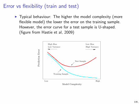
Error vs flexibility (train and test)
I Typical behaviour: The higher the model complexity (moreflexible model) the lower the error on the training sample.However, the error curve for a test sample is U-shaped.(figure from Hastie et al, 2009)
38 2. Overview of Supervised Learning
PSfrag replacements
High Bias
Low Variance
Low Bias
High Variance
Pre
dic
tion
Err
or
Model Complexity
Training Sample
Test Sample
Low High
FIGURE 2.11. Test and training error as a function of model complexity.
be close to f(x0). As k grows, the neighbors are further away, and thenanything can happen.
The variance term is simply the variance of an average here, and de-creases as the inverse of k. So as k varies, there is a bias–variance tradeoff.
More generally, as the model complexity of our procedure is increased,the variance tends to increase and the squared bias tends to decreases.The opposite behavior occurs as the model complexity is decreased. Fork-nearest neighbors, the model complexity is controlled by k.
Typically we would like to choose our model complexity to trade biasoff with variance in such a way as to minimize the test error. An obviousestimate of test error is the training error 1
N
∑i(yi − yi)
2. Unfortunatelytraining error is not a good estimate of test error, as it does not properlyaccount for model complexity.
Figure 2.11 shows the typical behavior of the test and training error, asmodel complexity is varied. The training error tends to decrease wheneverwe increase the model complexity, that is, whenever we fit the data harder.However with too much fitting, the model adapts itself too closely to thetraining data, and will not generalize well (i.e., have large test error). In
that case the predictions f(x0) will have large variance, as reflected in thelast term of expression (2.46). In contrast, if the model is not complexenough, it will underfit and may have large bias, again resulting in poorgeneralization. In Chapter 7 we discuss methods for estimating the testerror of a prediction method, and hence estimating the optimal amount ofmodel complexity for a given prediction method and training set.
135 ,

Curse of dimensionality
I For practicality, we illustrated kNN with 2-dimensional figures
I In practice, the dimensionality is usually much higher
I The number of samples required to get a good coverage of ad-dimensional domain is exponential in d
I For example, to cover a d-dimensional unit cube X = [0, 1]d
with a grid, with interval ε between grid points, we needroughly ε−d grid points
I Nearest neighbour methods often still work in highdimensional spaces, but it’s not as obvious as one might thinkfrom looking at 2-dimensional pictures
I The same issue appears in many other learning situations
136 ,

Analogous problem: Curve fitting
I Which of the following curves ‘fits best’ to the data?
137 ,

Analogous problem: Curve fitting
I Which of the following curves ‘fits best’ to the data?
137 ,
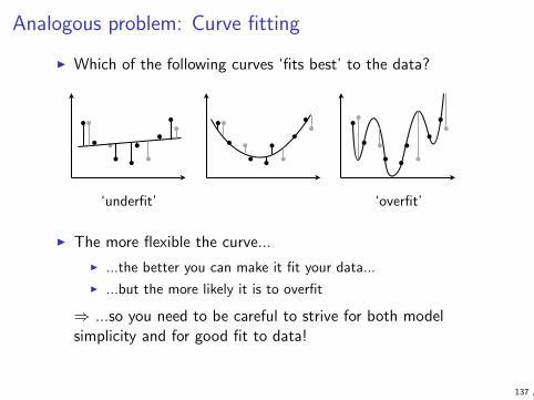
Analogous problem: Curve fitting
I Which of the following curves ‘fits best’ to the data?
‘underfit’ ‘overfit’
I The more flexible the curve...
I ...the better you can make it fit your data...
I ...but the more likely it is to overfit
⇒ ...so you need to be careful to strive for both modelsimplicity and for good fit to data!
137 ,

Bias-variance tradeoff
I Based on N training datapoints from the distribution, howclose is the learned classifier to the optimal classifier?
Consider multiple trials: repeatedly and independently drawingN training points from the underlying distribution.
I Bias: how far the average model (over all trials) is from thereal optimal classifier
I Variance: how far a model (based on an individual trainingset) tends to be from the average model
I Goal: Low bias and low variance.
I High model complexity ⇒ low bias and high varianceLow model complexity ⇒ high bias and low variance
138 ,

Bias-variance for regression
I Bias and variance have a particular mathematical meaning inregression with square loss
I Let fS : X → R be the model our algorithm produces fromtraining set S
I Let f∗(x) be the prediction of some “target” function f∗ (say,Bayes optimal)
I The loss of f with respect to the target on a given point x is
(f∗(x)− fS(x))2
I Taking expectation over all possible training sets gives
ES [(f∗(x)− fS(x))2]
139 ,
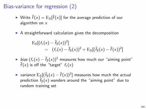
Bias-variance for regression (2)
I Write f (x) = ES [f (x)] for the average prediction of ouralgorithm on x
I A straightforward calculation gives the decomposition
ES [(f∗(x)− fS(x))2]
= (f∗(x)− fS(x))2 + ES [(fS(x)− f (x))2]
I bias (f∗(x)− fS(x))2 measures how much our “aiming point”f (x) is off the “target” f∗(x)
I variance ES [(fS(x)− f (x))2] measures how much the actualprediction fS(x) wanders around the “aiming point” due torandom training set
140 ,

Model complexity in decision trees(Discussed soon in more detail!)
I What is the appropriate size of the tree?
A
x1
x2
0 1 2 3 4 50
1
2
3
x1 > 2.8
I Use pre-pruning (stop ‘early’ before adding too many nodes)or post-pruning (after the full tree is constructed, try toimprove it by removing nodes)
141 ,

Model complexity in decision trees(Discussed soon in more detail!)
I What is the appropriate size of the tree?
A
B
x1
x2
0 1 2 3 4 50
1
2
3
x1 > 2.8
x2 > 2.0
I Use pre-pruning (stop ‘early’ before adding too many nodes)or post-pruning (after the full tree is constructed, try toimprove it by removing nodes)
141 ,

Model complexity in decision trees(Discussed soon in more detail!)
I What is the appropriate size of the tree?
A
B
B
x1
x2
0 1 2 3 4 50
1
2
3
x1 > 2.8
x2 > 2.0x2 > 1.2
I Use pre-pruning (stop ‘early’ before adding too many nodes)or post-pruning (after the full tree is constructed, try toimprove it by removing nodes)
141 ,

Model complexity in decision trees(Discussed soon in more detail!)
I What is the appropriate size of the tree?
A
B
B
Cx1
x2
0 1 2 3 4 50
1
2
3
x1 > 2.8
x2 > 2.0x2 > 1.2
x1 > 4.3
I Use pre-pruning (stop ‘early’ before adding too many nodes)or post-pruning (after the full tree is constructed, try toimprove it by removing nodes)
141 ,

Model complexity in decision trees(Discussed soon in more detail!)
I What is the appropriate size of the tree?
A
B
B
Cx1
x2
0 1 2 3 4 50
1
2
3
x1 > 2.8
x2 > 2.0x2 > 1.2
x1 > 4.3x1 > 2.2
I Use pre-pruning (stop ‘early’ before adding too many nodes)or post-pruning (after the full tree is constructed, try toimprove it by removing nodes)
141 ,
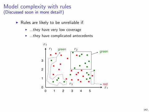
Model complexity with rules(Discussed soon in more detail!)
I Rules are likely to be unreliable if:
I ...they have very low coverage
I ...they have complicated antecedents
x1
x2
0 1 2 3 4 50
1
2
3
green
red
r1 r2
r3
green
142 ,
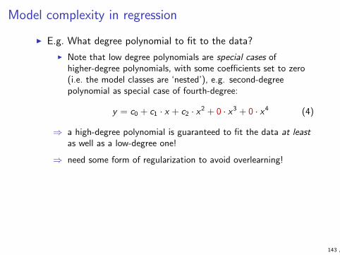
Model complexity in regression
I E.g. What degree polynomial to fit to the data?
I Note that low degree polynomials are special cases ofhigher-degree polynomials, with some coefficients set to zero(i.e. the model classes are ‘nested’), e.g. second-degreepolynomial as special case of fourth-degree:
y = c0 + c1 · x + c2 · x2 + 0 · x3 + 0 · x4 (4)
⇒ a high-degree polynomial is guaranteed to fit the data at leastas well as a low-degree one!
⇒ need some form of regularization to avoid overlearning!
143 ,
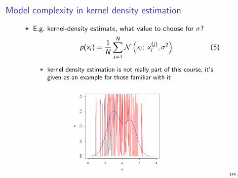
Model complexity in kernel density estimation
I E.g. kernel-density estimate, what value to choose for σ?
p(xi ) =1
N
N∑
j=1
N(
xi ; x(j)i , σ2
)(5)
I kernel density estimation is not really part of this course, it’sgiven as an example for those familiar with it
0 2 4 6 8
0.0
0.1
0.2
0.3
0.4
xi
fe
144 ,
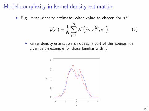
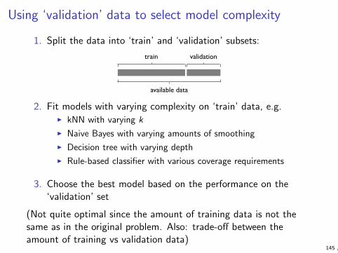
Using ‘validation’ data to select model complexity
1. Split the data into ‘train’ and ‘validation’ subsets:
train validation
available data
2. Fit models with varying complexity on ‘train’ data, e.g.I kNN with varying k
I Naive Bayes with varying amounts of smoothing
I Decision tree with varying depth
I Rule-based classifier with various coverage requirements
3. Choose the best model based on the performance on the‘validation’ set
(Not quite optimal since the amount of training data is not thesame as in the original problem. Also: trade-off between theamount of training vs validation data)
145 ,

Cross-validation
To get more reliable statistics than a single ‘split’ provides, useK -fold cross-validation:
1. Divide the data into K equal-sized subsets:
available data
1 2 3 4 5
2. For j goes from 1 to K :
2.1 Train the model(s) using all data except that of subset j
2.2 Compute the resulting validation error on the subset j
3. Average the K results
When K = N (i.e. each datapoint is a separate subset) this isknown as leave-one-out cross-validation.
146 ,
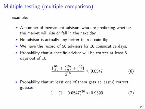
Multiple testing (multiple comparison)
Example:
I A number of investment advisors who are predicting whetherthe market will rise or fall in the next day.
I No advisor is actually any better than a coin-flip
I We have the record of 50 advisors for 10 consecutive days.
I Probability that a specific advisor will be correct at least 8days out of 10:
(108
)+(10
9
)+(10
10
)
210≈ 0.0547 (6)
I Probability that at least one of them gets at least 8 correctguesses:
1− (1− 0.0547)50 ≈ 0.9399 (7)
147 ,

I The moral of the story: If you are comparing a number ofrandom predictors, it is likely that some will have very goodempirical performance even if they are all quite random.
I It makes sense to select the best predictors, but one shouldnot have much faith in their predictive power unless one afterselection tests them on a fresh dataset
I This problem is strongly related to machine learning:
1. Many machine learning algorithms employ multiple tests whenselecting nodes to split or variables to include in the analysis
2. Overall, data mining is concerned with finding interesting anduseful relationships in data, and if the search is not restricted itis almost always possible to find ‘strange patterns’, even incompletely random data.
I The importance of this issue cannot be overstated!
148 ,

Estimating generalization performance
I So, at the end, to get an unbiased estimate of thegeneralization performance, test it on data that has not beenused in any way to guide the search for the best model. (Thetest data should be ‘locked in a vault’. No peeking!)
I If you are testing several models, beware that the best/worstresults may not be good estimates of the generalization errorof those models. (Don’t fall into that trap, again!)
I Often, data is divided in three: ‘train’, ‘validation’, and ‘test’
train validation
available data
test
I Can use a cross-validation approach for train/validation,but no peeking at the test data!
149 ,

Explicitly penalizing complexity
I Models can be regularized by explicitly adding a term thatpenalizes for complexity, as in
(model score) = (model fit to data)− λ · (model complexity)
where the fit to data can be likelihood, classification accuracy,or similar, and the model complexity can be
I Number of nodes in a decision tree
I Norm of the weights (parameters) of the model
I ...
I But how to select λ?Cross-validation, Bayesian approach, MDL, BIC, AIC...
150 ,
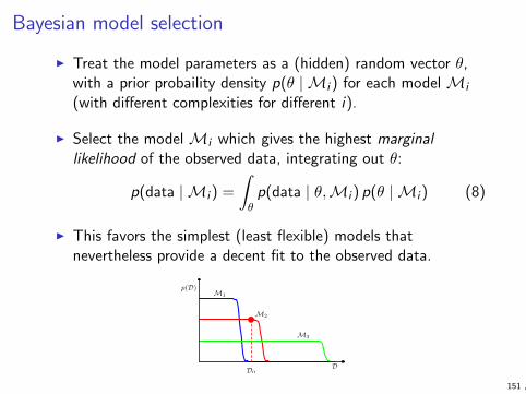
Bayesian model selection
I Treat the model parameters as a (hidden) random vector θ,with a prior probaility density p(θ | Mi ) for each model Mi
(with different complexities for different i).
I Select the model Mi which gives the highest marginallikelihood of the observed data, integrating out θ:
p(data | Mi ) =
∫
θp(data | θ,Mi ) p(θ | Mi ) (8)
I This favors the simplest (least flexible) models thatnevertheless provide a decent fit to the observed data.
p(D)
DD0
M1
M2
M3
151 ,

Minimum description length (MDL)
I Basic idea: The best ‘model’ for the data is the most compact(shortest) description of the data
I Typically, this will consist of describing some generalcharacteristics of the data, and then the details of how thedata deviates from those predictions:
L(description of model) + L(description of data given the model)
I Thus, this framework provides one way of balancing modelcomplexity with data fit (but the devil is in the details)
I For a thorough treatment, take the course‘Information-Theoretic Modeling’
152 ,
Decision trees and rule-based classifiers
153 ,

Decision tree: An example
I Idea: Ask a sequence of questions (as in the ‘20 questions’game) to infer the class
includes ‘netflix prize’includes ‘viagra’
includes ‘millions’
includes ‘meds’
no yes
not spamspam
yes
spam
yes nono
spam
yesno
not spam
154 ,

Decision tree: A second example
!"#$%&'()*%+$,-&"./0$1" 2%(134/,(*3%"(3"5$($"6*%*%7"""""""" 89:;9<==8""""""""""""""">
!"#$$%&%'#(%)*+,-'.*%/0-$
5),*?*3%"#1))"+$?)4"6)(-34?@/A)B+$?)4"6)(-34?6)031C"+$?)4"1)$?3%*%7D)/1$A"D)(E31F?D$GH)"I$C)? $%4"I$C)?*$%"I)A*)J"D)(E31F?'/KK31("L),(31"6$,-*%)?
!"#$%&'()*%+$,-&"./0$1" 2%(134/,(*3%"(3"5$($"6*%*%7"""""""" 89:;9<==8"""""""""""""""M
12#34"-+)&+#+5-'%$%)*+,6--
!"# !"#$%& '()*+(,-+(+$.
/(0(1,"2%345" 67"(+
: N)? '*%7A) :<>. 84
< D3 6$11*)4 :==. 84
O D3 '*%7A) P=. 84
8 N)? 6$11*)4 :<=. 84
> D3 5*H31,)4 Q>. 9".
M D3 6$11*)4 M=. 84
P N)? 5*H31,)4 <<=. 84
; D3 '*%7A) ;>. 9".
Q D3 6$11*)4 P>. 84
:= D3 '*%7A) Q=. 9".:=
3(+":4)*3(,
3(+":4)*3(,
34%+*%$4$.
3,(..
!"#$%&
'()-+
/(02%3
9;-8<
8<
8<
N)? D3
6$11*)4'*%7A)&"5*H31,)4
R";=. S";=.
!"#$%%$&'()%%*$+,%-.
/)(*%*%:=>(+( '4&",?==>"3*.*4%=/)""
I There can be many different trees that all work equally well!
155 ,
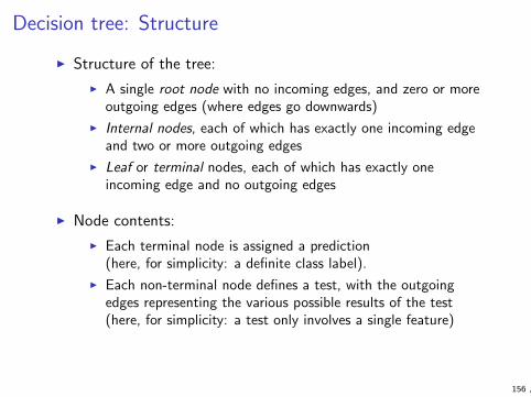
Decision tree: Structure
I Structure of the tree:
I A single root node with no incoming edges, and zero or moreoutgoing edges (where edges go downwards)
I Internal nodes, each of which has exactly one incoming edgeand two or more outgoing edges
I Leaf or terminal nodes, each of which has exactly oneincoming edge and no outgoing edges
I Node contents:
I Each terminal node is assigned a prediction(here, for simplicity: a definite class label).
I Each non-terminal node defines a test, with the outgoingedges representing the various possible results of the test(here, for simplicity: a test only involves a single feature)
156 ,
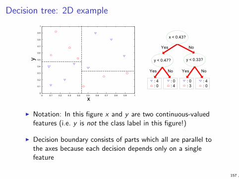
Decision tree: 2D example
!"#$%&'()*%+$,-&"./0$1" 2%(134/,(*3%"(3"5$($"6*%*%7"""""""" 89:;9<==8""""""""""""""">:
!"#$%$&'()&*'+,-.
?"@"=ABBC
"""""D"="""""D"B
"""""D"8"""""D"=
?"@"=A8>C
""""D"8""""D"=
"""""D"="""""D"8
E"@"=A8BC
F)G
F)G
H3
H3 F)G H3
= =A: =A< =AB =A8 =AI =AJ =A> =A; =AK :=
=A:
=A<
=AB
=A8
=AI
=AJ
=A>
=A;
=AK
:
E
?
L !"#$%#&'()%&*%+,%%)&+,"&)%(-.*"#()-&#%-(")/&"0&$(00%#%)+&1'2//%/&(/&3)",)&2/&$%1(/(")&*"4)$2#5
L 6%1(/(")&*"4)$2#5&(/&72#2''%'&+"&28%/&*%124/%&+%/+&1")$(+(")&()9"'9%/&2&/()-'%&2++#(*4+%&2+:2:+(;%
!"#$%&'()*%+$,-&"./0$1" 2%(134/,(*3%"(3"5$($"6*%*%7"""""""" 89:;9<==8"""""""""""""""><
/01$2*"(!"#$%$&'(3-""%
8&<&5&=&>
?'2//&@&< ?'2//&@&&&&&
L A%/+&1")$(+(")&;25&()9"'9%&;4'+(7'%&2++#(*4+%/
L B"#%&%87#%//(9%&#%7#%/%)+2+(")
L C()$()-&"7+(;2'&+%/+&1")$(+(")&(/&1";74+2+(")2''5&%87%)/(9%
I Notation: In this figure x and y are two continuous-valuedfeatures (i.e. y is not the class label in this figure!)
I Decision boundary consists of parts which all are parallel tothe axes because each decision depends only on a singlefeature
157 ,
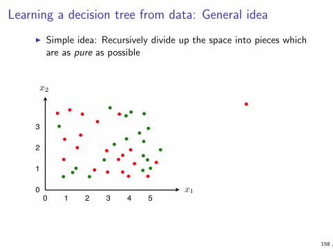
Learning a decision tree from data: General idea
I Simple idea: Recursively divide up the space into pieces whichare as pure as possible
x1
x2
0 1 2 3 4 50
1
2
3
158 ,

Learning a decision tree from data: General idea
I Simple idea: Recursively divide up the space into pieces whichare as pure as possible
A
x1
x2
0 1 2 3 4 50
1
2
3
x1 > 2.8
158 ,

Learning a decision tree from data: General idea
I Simple idea: Recursively divide up the space into pieces whichare as pure as possible
A
B
x1
x2
0 1 2 3 4 50
1
2
3
x1 > 2.8
x2 > 2.0
158 ,
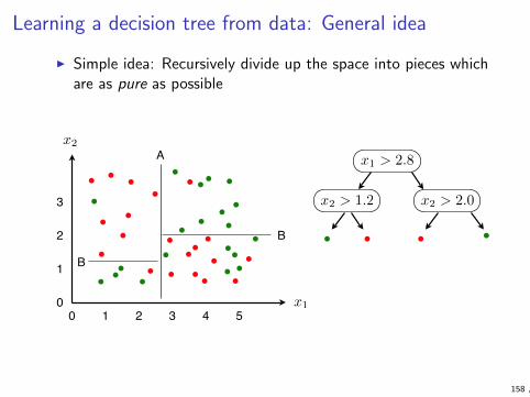
Learning a decision tree from data: General idea
I Simple idea: Recursively divide up the space into pieces whichare as pure as possible
A
B
B
x1
x2
0 1 2 3 4 50
1
2
3
x1 > 2.8
x2 > 2.0x2 > 1.2
158 ,

Learning a decision tree from data: General idea
I Simple idea: Recursively divide up the space into pieces whichare as pure as possible
A
B
B
Cx1
x2
0 1 2 3 4 50
1
2
3
x1 > 2.8
x2 > 2.0x2 > 1.2
x1 > 4.3
158 ,
Learning a decision tree from data: basic algorithm
I Notation: Let D denote the set of examples corresponding toa node t. For the root node, D is the set of all training data.
I Basic algorithm:
1. If all examples in D belong to the same class y , then t is a leafnode labelled as y
2. If D contains examples that belong to more than one class,select a feature test that partitions D into smaller subsets.Create a child node for each outcome and distribute theexamples in D to the children. Apply the algorithm recursivelyto each child node.
If D is an empty set: use majority vote among parent records (thismay happen for non-binary features)
If all instances in D are identical, but labels not: use majority vote
159 ,
Learning a decision tree (cont.)
I Previous algorithm is given more formally as Algorithm 5.1 intext book
I routines Homogeneous and Label can be used to refine Step 1
I routine BestSplit explains selecing feature test in Step 2
We’ll discuss these routines next, starting with BestSplitwhich is the most interesting
I This algorithm is known as Hunt’s algorithm, or TDIDT(Top-Down Induction of Decision Trees, where “induction” isa term historically used in particular for learning logicalmodels)
160 ,

Feature test conditions
I Binary features: yes / no (two children only)
I Nominal (categorical) features with L values:
I Multiway split (L children)
I Binary split (2 children, any of the 2L−1 − 1 ways of splitting)
I Ordinal features with L states:
I Multiway or binary split
I Must respect the ordering (only combine contiguous values)
I Continuous features:
I Multiway or binary split
I Defined using breakpoints
161 ,
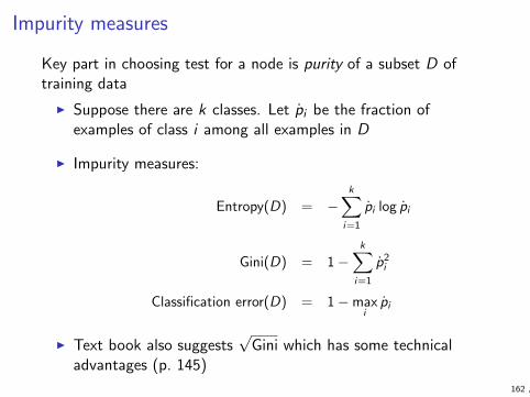
Impurity measures
Key part in choosing test for a node is purity of a subset D oftraining data
I Suppose there are k classes. Let pi be the fraction ofexamples of class i among all examples in D
I Impurity measures:
Entropy(D) = −k∑
i=1
pi log pi
Gini(D) = 1−k∑
i=1
p2i
Classification error(D) = 1−maxi
pi
I Text book also suggests√
Gini which has some technicaladvantages (p. 145)
162 ,

Impurity measures: Binary classification
0.0 0.2 0.4 0.6 0.8 1.0
0.0
0.1
0.2
0.3
0.4
0.5
p0
entropy
Entropy/2
Gini
Misclassification error
I Qualitatively, the three measures agree. However, somedifferences in the selection of test features do occur.
163 ,

Selecting the best split
I Let Imp(D) be impurity of data set D
I Assume a given feature test has m possible values and splitsD into subsets D1, . . . ,Dm
I We define the impurity of this split as
Imp({D1, . . . ,Dm }) =m∑
i=1
|Di ||D| Imp(Di )
and the related gain as
Imp(D)− Imp({D1, . . . ,Dm })
I BestSplit considers all possible splits using available featuresand returns the one with highest gain (or equivalently lowestimpurity)
164 ,

When to stop recursing
I We assume Homogeneous returns true iff all examples in Dbelong to same class
I It would be possible to stop recursion if D is “homogeneousenough” but still contains different classes. This is known aspre-pruning but generally not recommended
I In contrast, post-pruning (called simply pruning in text book,see pp. 142–143) is an additional step to simplify the tree afterit has first been fully grown to have only single-class leaves
I Reduced error pruning (Algorithm 5.3) is a commonly usedpost-pruning method
I usually increases understandability to humans
I typically increases generalisation performance
165 ,

Reduced-error pruning
I Withhold part of training data as pruning set
I Create a decision tree with single-class leaves using the rest oftraining data
I Repeat the following until there are no changes:I Pick the deepest internal node t
I If replacing the tree rooted t with a single leaf would increaseaccuracy on pruning set, do so
I Notice that you have now used the pruning set for learning.You cannot then re-use the pruning set as test set.
166 ,

Choosing the leaf prediction
I For simple classification, Label simply returns the majorityclass of the examples associated with the node
I However we can also create probabilitistic classifiers
I Notation:I classes c1, . . . , ckI data set D in the node contains ni instances with label ci , with
n =∑
i ni
I the predicted class distribution for instances associated withthe leaf is p = (p1, . . . , pk)
I So, how do we choose p based on n?
167 ,

Choosing the leaf label (cont.)
I The obvious choice is the empirical probabilities:
pi =ni
n
I However we get smoother and more stable estimates byapplying Laplace correction
pi =ni + 1
n + k
I More generally, we may assign to each class ci a pseudo-countmi , so
pi =ni + mi
n + m
where m =∑
i mi (see p. 75 of textbook)
168 ,
Choosing the leaf label (cont.)
I These techniques are commonly used for estimating adistribution, but decision trees are particularly challenging:
I data set in a single leaf can be very small
I class distribution in a leaf is very skewed
I Probabilistic binary classifier can then be easily used to get aranker
I rank the leaves in increasing probability of class +
I instances associated with the same leaf get same rank
I Finally, can turn ranker into classifier as usualI possible to tune for skewed class distribution or cost (slides
116–117, pages 69–72 in book)
169 ,
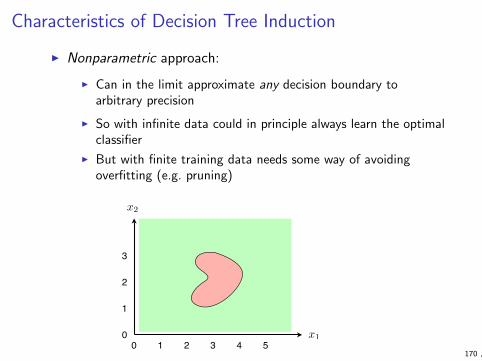
Characteristics of Decision Tree Induction
I Nonparametric approach:
I Can in the limit approximate any decision boundary toarbitrary precision
I So with infinite data could in principle always learn the optimalclassifier
I But with finite training data needs some way of avoidingoverfitting (e.g. pruning)
x1
x2
0 1 2 3 4 50
1
2
3
170 ,
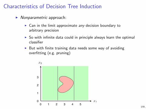
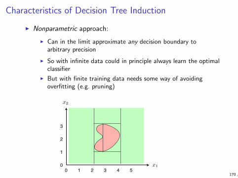
Characteristics of Decision Tree Induction (cont.)
I Local, greedy learning to find a reasonable solution inreasonable time (as opposed to finding a globally optimalsolution)
I Relatively easy to interpret (by experts or regular users of thesystem)
171 ,

Characteristics of Decision Tree Induction (cont.)
I Data fragmentation problem:I The nodes far down the tree are based on a very small fraction
of the data, even only on a few data points ⇒ typically notvery reliable information
I Example: Divide any of the existing leaves into purerpartitions:
A
B
B
Cx1
x2
0 1 2 3 4 50
1
2
3
x1 > 2.8
x2 > 2.0x2 > 1.2
x1 > 4.3
172 ,

Comments on decision trees in text book
I Traditional approach to decision tree learning is buildingdirectly a (deterministic) classifier with zero training error andthen using reduced error pruning
I Text book recommends (p. 147) building first a probabilisticclassifier and then using standard techniques, which is a muchmore recent approach
I In this course we have de-emphasise the ranking part just inthe interest of simplicity
I We don’t have time here to cover regression and clusteringtrees (Section 5.3) at all
173 ,

Rule-based classifier
I e.g. Mac OS X ‘Mail’ application:
174 ,

What is a rule
I Examples of rules for classification:I if (Income < 30000) ∧ (OwnsHouse = false) then NoLoan
I if (’important’) ∧ (Sender = Teacher) then NoSpam
I Terminology:I if-part is called body or antecedent; in classification this is
some (simple) test based on feature values
I then-part is called head or consequence; in classification this isa class
175 ,

Properties of a single rule
I If the head of a rule is true for a given instance, we say therule covers the instance, and the instance matches the rule
I Given a set of (labelled or unlabelled) instances, the coverageof a rule is the fraction of instances that are covered
I Given a set of labelled instances, the accuracy of a rule isobtained by considering only covered instances and observingthe proportion of them where the label matches the head ofthe rule
I Ideally, we want good coverage and good accuracy
I However, a single rule cannot usually achieve both (withoutmaking the body too complicated)
I hence we consider rule sets
176 ,

Properties of a rule set
I If all possible instances are covered by at least one rule, therule set is complete (or exhaustive)
I If no instance is covered by more than one rule, the rule set ismutually exclusive
I If no instance is covered by two rules where the head(classification) is different, the rule set is consistent
I Notice that here we are talking about all imaginable instancesin the instance space, not just those in training set etc.
I Generally we learn rule sets that are complete and have someprocedure for dealing with inconsistencies
177 ,

Ordered rule lists
I In an ordered rule list, the rules are listed in order
I The classification is determined by the first rule that coversthe instance
I The rule list is usually made complete by adding last a defaultrule such as
if true then class = ’+’
I Advantage: clear procedure for inconsistencies
I Disadvantage: meaning of a single rule less easy tounderstand since it depends on all preceding rules
I Ordered rule sets are also called decision lists
178 ,

Learning an ordered rule list
I Start with an empty list
I Repeat the following until no data remainsI Find a rule with good accuracy
I Add the rule to the end of list
I Remove all data points that are covered by the rule
I Change the last rule into a default rule (if it is not already)
179 ,
Finding a good rule
I The most common method is to start with the antecedent setto true and add to it more conditions one by one until astopping criterion is met
I Conditions are tests for a value of a single feature, which arecalled literals in textbook
I At each step, we greedily choose the literal that results inlargest increase in some purity measure (similar to decisiontrees)
I Usual stopping criteria include the number of data pointsdropping below a given threshold, or the data set becomingsufficiently pure
180 ,
Learning unordered rule sets
I The text book gives an example of how we can modify theprevious algorithm to create unordered rule sets
I Instead of creating a single ordered list, we create a separateunordered rule set for each class
I Unlike with ordered rules, when we add a new rule for class ci ,we cannot remove examples that belong to other classescj 6= ci
I also the rules that will be added for class ci later in theprocedure need to avoid covering all examples from cj 6= ci bythemselves
I Notice that the final combined rule set may still beinconsistent; we’ll get back to that
181 ,

Finding rules for unordered sets
I We can use a similar basic approach where we add featuretests to the body one by one
I Since we now know which class we are aiming for, we canguide the search by classification accuracy for that classinstead of some general purity measure
182 ,

Variations to searching for a single rule
I pick a seed example of the appropriate class and limit searchto literals that it satisfies
I instead of just greedily going to the best candidate, keep afixed-size pool of candidates (beam search)
I There is a huge body of literature on search heuristics indecision tree and rule learning; see references in text book forstarting points if you are interested
183 ,
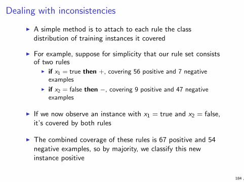
Dealing with inconsistencies
I A simple method is to attach to each rule the classdistribution of training instances it covered
I For example, suppose for simplicity that our rule set consistsof two rules
I if x1 = true then +, covering 56 positive and 7 negativeexamples
I if x2 = false then −, covering 9 positive and 47 negativeexamples
I If we now observe an instance with x1 = true and x2 = false,it’s covered by both rules
I The combined coverage of these rules is 67 positive and 54negative examples, so by majority, we classify this newinstance positive
184 ,

Rules in text book
I Text book covers rule learning algorithms in more detail thanwe did here, but not in enough detail for actuallyimplementing one
I For more details, follow up on references in Section 6.5
I In any case, instead of implementing yourself you should useexisting packages if possible
I We did not cover here using rules for ranking and probabilisticprediction; the basic idea is similar to decision trees, but thereare differences
I We also didn’t cover descriptive rule learning
185 ,

Decision trees and rule-based classifiers: Summary
I Can be easy to understand/interpret by experts/users (forsmall models)
I Classification generally very fast (worst case is linear in depthof decision tree or rule list length)
I Non-parametric method (can approximate optimal classifierfor any underlying distribution) in the large sample limit (butmay require a very large number of rules)
I Need to control complexity when learning to avoid overfitting
186 ,

Linear models
187 ,

Linear models
I We consider the case x ∈ Rd throughout this chapter
I Function f : Rd → R is linear if for some w ∈ Rd it can bewritten as
f (x) = w · x =d∑
j=1
wjxj
and affine if for some w ∈ Rd and a ∈ R we can write
f (x) = w · x + a
I w is often called weight vector and a is called intercept (orparticularly in machine learning literature, bias)
188 ,
Linear models (2)
I Linear model generally means using an affine function by itselffor regression, or as scoring function for classification
I The learning problem is to determine the parameters w and abased on data
I Linear regression and classification have been extensivelystudies in statistics
189 ,

Univariate linear regression
I As warm-up, we consider linear regression in one-dimensionalcase d = 1
I We use square error and want to minimise it on training set(x1, y1), . . . , (xn, yn)
I Thus, we want to find a,w ∈ R that minimise
E (w , a) =n∑
i=1
(yi − (wxi + a))2
I This is known as ordinary least squares and can be motivatedas maximum likelihood estimate for (w , a) if we assume
yi = wxi + a + ηi
where ηi are i.i.d. Gaussian noise with zero mean
190 ,

Univariate linear regression (2)
I We solve the minimisation problem by setting the partialderivatives to zero
I We denote the solution by (w , a)
I We have∂E (w , a)
∂a= −2
n∑
i=1
(yi − wxi − a)
and setting this to zero gives
a = y − wx
where y = (1/n)∑
i yi and x = (1/n)∑
i xi
I This implies in particular that the point (x , y) is on the liney = wx + a
191 ,

Univariate linear regression (3)
I Further,∂E (w , a)
∂w= −2
n∑
i=1
xi (yi − wxi − a)
I Plugging in a = a and setting the derivative to zero gives us
n∑
i=1
xi (yi − wxi − y + wx) = 0
from which we can solve
w =
∑Ni=1 xi (yi − y)
∑Ni=1 xi (xi − x)
192 ,

Univariate linear regression (4)
I Sincen∑
i=1
x(yi − y) = x
(n∑
i=1
yi − ny
)= 0
andn∑
i=1
x(xi − x) = x
(n∑
i=1
xi − nx
)= 0
we can finally rewrite this as
w =
∑Ni=1(xi − x)(yi − y)∑N
i=1(xi − x)2
I Notice that we have w = σxy/σxx where σpq is samplecovariance between p and q:
σpq =1
n − 1
n∑
i=1
(pi − p)(qi − q)
193 ,
Useful trick
I In more general situation than univariate regression, it wouldoften be simpler to learn just linear functions and not worryabout the intercept term
I An easy trick for this is to replace each instancex = (x1, . . . , xd) ∈ Rd by x′ = (1, x1, . . . , xd) ∈ Rd+1
I Now an affine function f (x) = w · x + a in Rd becomes linearfunction g(x ′) = w′ · x′ where w′ = (a,w1, . . . ,wd)
I If we write the set of instances x1, . . . , xn as an n × d matrix,this means adding an extra column of ones
I This is known as using homogeneous coordinates (textbook p.24)
194 ,

Useful trick (2)
I For most part we now present algorithms for learning linearfunctions (instead of affine)
I In practice, to run them on d-dimensional data, we add thecolumn of ones and run the algorithm in d + 1 dimensions
I The first component of w then gives the intercept
I However sometimes we might still want to treat the interceptseparately (for example in regularisation)
195 ,

Multivariate linear regression
I We now move to the general case of learning a linear functionRd → R for arbitrary d
I As discussed above, we omit the intercept
I We still use the square loss, which is by far the mostcommonly used loss for linear regression
I One potential problem with square loss is its sensitivity tooutliers
I one alternative is absolute loss∣∣∣y − f (x)
∣∣∣I computations become trickier with absolute loss
196 ,

Multivariate linear regression (2)
I We assume matrix X ∈ Rn×d has n instances xi as its rowsand y ∈ Rn contains the corresponding labels yi
I We writey = Xw + ε
where the residual εi = yi −w · xi indicates error that weightvector w makes on data point (xi , yi )
I Our goal is to find w which minimises the sum of squaredresiduals
n∑
i=1
ε2i = ‖ε‖2
2
197 ,

Multivariate linear regression (4)
I Write y0 = Xw, so our goal is to minimise ‖ε‖2 = ‖y − y0‖2
I Since w ∈ Rd can be anything, y0 can be any vector in thelinear span S of the columns of X
I In other words, y0 ∈ S = span(c1, . . . , cd) wherecj = (x1j , . . . , xdj) is jth column of X and
span(c1, . . . , cd) ={
w1c1 + · · ·+ wdcd) | w ∈ Rd}
198 ,

Multivariate linear regression (5)
I Since S is a linear subspace of Rn, the minimum of ‖y − y0‖2
subject to y0 ∈ S occurs when y0 is the projection of y to S
I Therefore in particular y · cj = y0 · cj for j = 1, . . . , d
I Since y · cj = (XTy)j , we write this in matrix form as
XTy = XTy0 = XTXw
where we have substituted back y0 = Xw
I Multiplying both sides by (XTX)−1 gives the solution
w = (XTX)−1XTy
199 ,

Multivariate linear regression (6)
I If the columns cj of X are linearly independent, the matrixXTX is of full rank and has an inverse
I For n > d this is true except for degenerate special cases
I XTX is a d × d matrix, and inverting it takes O(d3) time
I For very high dimensional problems the computation time maybe prohibitive
200 ,
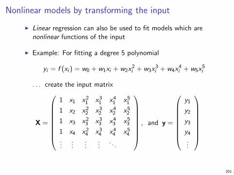
Nonlinear models by transforming the input
I Linear regression can also be used to fit models which arenonlinear functions of the input
I Example: For fitting a degree 5 polynomial
yi = f (xi ) = w0 + w1xi + w2x2i + w3x3
i + w4x4i + w5x5
i
. . . create the input matrix
X =
1 x1 x21 x3
1 x41 x5
1
1 x2 x22 x3
2 x42 x5
2
1 x3 x23 x3
3 x43 x5
3
1 x4 x24 x3
4 x44 x5
4
......
......
. . .
, and y =
y1
y2
y3
y4
...
201 ,

Nonlinear predictors by transforming the input (2)
I We can also explicitly include some interaction terms, as in
yi = f (xi ) = w0 + w1xi1 + w2xi2 + w3xi1xi2
using the following input matrix:
X =
1 x11 x12 x11x12
1 x21 x22 x21x22
1 x31 x32 x31x32
1 x41 x42 x41x42
......
......
, and y =
y1
y2
y3
y4
...
202 ,

Regularised regression
I If dimensionality d is high, linear models are actually quiteflexible
I We can avoid overfitting by minimising not just the squarederror ‖y − Xw‖2
2 but the regularised cost
‖y − Xw‖22 + λ ‖w‖2
2
where λ > 0 is a constant (chosen e.g. by cross validation)
I By increasing λ we decrease variance but increase bias
I This allows us to sometimes get sensible results even in thecase n < d
203 ,
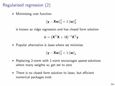
Regularised regression (2)
I Minimising cost function
‖y − Xw‖22 + λ ‖w‖2
2
is known as ridge regression and has closed form solution
w = (XTX + λI)−1XTy
I Popular alternative is lasso where we minimise
‖y − Xw‖22 + λ ‖w‖1
I Replacing 2-norm with 1-norm encourages sparse solutionswhere many weights wi get set to zero
I There is no closed form solution to lasso, but efficientnumerical packages exist
204 ,

Linear classification via regression
I As we just saw, minimising squared error in linear regressionhas a nice closed form solution (if inverting a d × d matrix isreasonable)
I In contrast, given a binary classification training set(x1, y1), . . . , (xn, yn) where yi ∈ {−1,+1 }, it iscomputationally intractable to find weight vector w whichminimises 0-1 loss
n∑
i=1
I [yiw · xi ≤ 0]
I One approach is to replace 0-1 loss I [yiw · xi ≤ 0] withsomething that is easier to optimise
205 ,

Linear classification via regression (2)
I In particular, we could replace I [yiw · xi ≤ 0] with(yi −w · xi )2
I learn w using least squares regression on the binaryclassification data set (with yi ∈ {−1,+1 })
I use w in linear classifier c(x) = sign(w · x + a) for somesuitable a ∈ R
I advantage: computationally efficient
I disadvantage: sensitive to outliers (in particular, havingyiw · xi � 1 gets heavily punished, which is counterintuitive)
I If we are willing to invert a d × d matrix, other well-knownalternatives can be found in statistics literature (Lineardiscriminant analysis LDA)
206 ,

The Perceptron algorithm
I The perceptron algorithm is a simple iterative method whichcan be used to train a linear classifier
I If the training data (xi , yi )ni=1 is linearly separable, i.e. there is
some w ∈ Rd such that yiw · xi > 0 for all i , the algorithm isguaranteed to find such a w
I The algorithm (or its variations) can be run also fornon-separable data but there is no guarantee about the result
I Even if the data is linearly separable, the perceptron algorithmis only guaranteed to converge in some finite time. Fordifficult problems, it may be very slow. A better worst-casebehavior is obtained by using linear programming (but theresult may not generalise well)
207 ,

Perceptron algorithm: Main ideas
I The algorithm keeps track of and updates a weight vector w
I Each input item is shown once in a sweep. If a full sweep iscompleted without any misclassifications then we are done,and return w that classifies all training data correctly. If Tsweeps are finished, we stop anyway and return whatever wwe ended up with.
I Whenever yi 6= yi we update w by adding yixi . This turns wtowards xi if yi = +1, and away from xi if yi = −1
I Note on terminology: a full sweep through the data is in thiscontext often called an epoch
208 ,

Perceptron algorithm: Illustration
training example of class +1training example of class –1
w
Current state of w
209 ,

Perceptron algorithm: Illustration
training example of class +1training example of class –1
w
Red point classified correctly, no change to w
209 ,
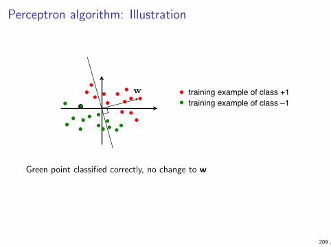
Perceptron algorithm: Illustration
training example of class +1training example of class –1
w
Green point classified correctly, no change to w
209 ,
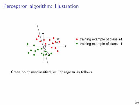
Perceptron algorithm: Illustration
training example of class +1training example of class –1
w
Green point misclassified, will change w as follows...
209 ,
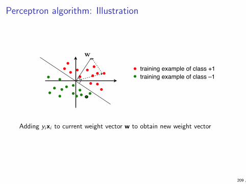
Perceptron algorithm: Illustration
training example of class +1training example of class –1
w
Adding yixi to current weight vector w to obtain new weight vector
209 ,

Perceptron algorithm: Pseudocode
w← 0for epoch = 1:T
converged ← truefor i = 1:N
yi ← sign(w · xi )if yi 6= yi
w← w + yixiconverged ← false
if converged ← truebreak
return w
210 ,

Comments on pseudocode
I We go through the data repeatedly until a linear classifierwith zero training error is found, or until a predefinedmaximum number of epochs T is reached
I The version in textbook goes to infinite loop if data is notlinearly separable
I The textbook version also includes an additional parameter η(called learning rate or step size) which is redundant for thisbasic version of the algorithm
211 ,

Online algorithms
I Perceptron is an online algorithm where examples areconsidered one at a time, and each time a small update is(possibly) made to the current hypothesis
I AdvantagesI individual update usually fast and easy to implement
I scales naturally to very large data sets
I can be used e.g. for data streams where individual data itemsarrive fast, must be processed immediately and cannot bestored
I DisadvantagesI may require several iterations through the data
I convergence difficult to analyse
212 ,

Online algorithms (2)
I More specifically, the Perceptron algorithm is an instance ofstochastic gradient descent (SGD)
I Generally, assuming a loss L(y ,w, x) for using parameters won instance x when correct label is y , the SGD update is
w ← w − η∇wL(yi ,w, xi )
where ∇ denotes gradient and η > 0 is a step size parameter
I Perceptron is obtained with L(y ,w, x) = max { 0,−yw · x }
I Applying same idea for least squares regression gives a famousalgorithm known as Least Mean Squares or Widrow-Hoff:
w ← w + η(yi −w · xi )xi(Algorithm 7.3 in textbook has incorrect update, use this oneinstead)
213 ,
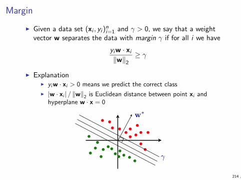
Margin
I Given a data set (xi , yi )ni=1 and γ > 0, we say that a weight
vector w separates the data with margin γ if for all i we have
yiw · xi‖w‖2
≥ γ
I ExplanationI yiw · xi > 0 means we predict the correct class
I |w · xi | / ‖w‖2 is Euclidean distance between point xi andhyperplane w · x = 0
w∗
γ
214 ,

Perceptron conergence theorem
I Consider a data set (xi , yi )ni=1 where ‖xi‖2 ≤ R for all i
I Assume there is some w that separates the data with marginγ > 0
I Then the Perceptron algorithm makes at most
R2
γ2
updates before converging
I Proof is straightforward linear algebra, but we omit it here
215 ,

Support vector machine (SVM)
I Hard margin SVM: assuming data is linearly separable, findsw with largest possible margin
I Soft margin SVM: regularised algorithm that works also onnon-separable data
I SVM is often used in combination with a kernel function:intuitively this allows learning non-linear models of certaintypes, where choice of kernel determines the type ofnonlinearity (e.g. polynomial)
I Computationally demanding, but efficient specialisedoptimisation software exist; training sets of at least tens ofthousands of examples can be handled by basic packages
I Details of SVMs are beyond the scope of this course
216 ,
Perceptron algorithm: Non-convergence
I If the training data is linearly separable, the perceptronalgorithm converges after a finite number of steps.
I However, the finite number can be very large if the margin isnot wide.
I If the training data is not linearly separable, the algorithmdoes not converge, because it simply cannot (by definition)get through a full sweep of the data without performing anupdate.
I What then?I Pocket algorithm can be added on top of the Perceptron
algorithm (or any other online classifier) to deal withnon-convergence
I Use an alternative linear classification algorithm: LDA, SVM,logistic regression [later in lectures], . . . )
217 ,
Perceptron algorithm: dealing with non-convergence
I If the Perceptron algorithm does not converge, how do youpick a final w to use on new data?
I Some methods that are generally useful for improvingconvergence of iterative algorithms can be useful
I Use a smaller learning rate, as in w← w + λyixi formisclassified points (xi , yi ), with λ > 0 decreasing for eachsweep
I Take a running average of recent weight vectors
I The Pocket Algorithm (Gallant 1990) is a simple method toget a final w when iterations don’t converge
218 ,

The Pocket algorithm
I Run Perceptron algorithm updating w as usual
I Keep a score for current w by simply counting how manycorrect predictions w has made in a row
I The algorithm has a “pocket” where it stores the weightvector wp that has had the highest score thus far, and itsscore scorep
I Initially wp = 0 and scorep = 0
I When a full epoch passes without the contents of the pocketchanging, the algorithm gives wp as its final result andterminates
219 ,

The Pocket algorithm (2)
Corresponding to each step i of the Perceptron algorithm
I if the prediction was correct (yiw · xi > 0)I increase score: score← score + 1
I otherwise (if yiw · xi ≤ 0)I if the previous high score was beaten, i.e. score > scorep, then
set wp ← w and scorep ← score
I update w← w + yixi as usual
I reset score← 0.
220 ,

Linear classifier for multiclass problem
I Linear classifier is directly applicable only to binaryclassification
I Multiclass problems can be tackled as follows:
1. For each class y ∈ Y create a two-class classification problemin which the task is to predict whether the true class is y (+1)or not (−1). The training data is obtained from the originaldata by changing the true classes into +1/− 1
2. Train the weights of a linear classifier wy for each class y withdata as above
3. To classify a new x, choose the class y for which wTy x is largest
I This method of reducing multiclass classification to binary isknown as one-versus-rest or 1-versus-all.
(See the example on next slide)
221 ,

Linear classifier for multiclass problem
training example of class Atraining example of class Btraining example of class C
wA
222 ,
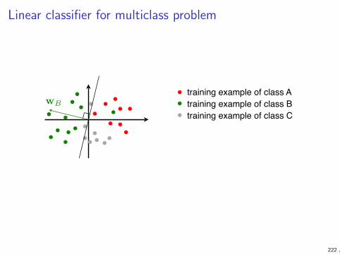
Linear classifier for multiclass problem
training example of class Atraining example of class Btraining example of class C
wB
222 ,

Linear classifier for multiclass problem
training example of class Atraining example of class Btraining example of class C
wC
222 ,
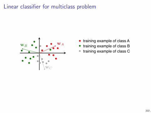
Linear classifier for multiclass problem
training example of class Atraining example of class Btraining example of class C
wC
wAwB
222 ,

Linear classifier for multiclass problem: alternatives
I A popular alternative to one-vs.-all is one-versus-one, alsoknown as all-versus-all
1. For each pair of distinct classes yi , yj ∈ Y create a modifiedtraining set by re-labeling class yi as + and yj as −. Ignoredata points from the other classes. Call the resulting weightvector wij . (Notice that in our case wij = −wji .)
2. To classify a new x, pick yi that maximizes∑
j sign(wij · x).
I It’s difficult to say theoretically whether 1-vs.-rest or 1-vs.-1gives a more accurate classifier.
I However the computational difference is significant: all-vs.-allrequires solving k(k − 1)/2 classifiers, where k = |Y|, but thetraining sets for the classifiers are smaller.
I There are also more complicated techniques such asError-Correcting Output Coding (ECOC)
223 ,
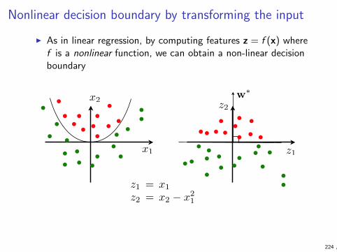
Nonlinear decision boundary by transforming the input
I As in linear regression, by computing features z = f (x) wheref is a nonlinear function, we can obtain a non-linear decisionboundary
w∗
x1
x2
z1
z2
z1 = x1
z2 = x2 − x21
224 ,

Linear models in machine learning
I Linear models are well studied in statistics literature, both forregression and classificatio
I Both statistical theory and optimisation algorithms are muchbetter understood for linear than for non-linear models
I However computer scientists need more expressive models todeal with tasks that are inherently non-linear
I Currently one of the main overall approaches is to introduce alarge number of non-linear features and use linear models onthe feature vectors
I often dones implicitly via kernel function (e.g. SVM)
I Leads to somewhat new territory for linear modelsI very high dimensional problems, need regularisation etc.
I new types of optimisation problems
225 ,

Linear models: what was important
I Algorithms:I least squares regression: fundamental technique, including
regularisation
I Perceptron: probably not the best algorithm in the world forany given task, but the starting point if you want tounderstand linear classification or online algorithms in general
I linear discriminant analysis, SVM: we didn’t have time to coverthese, but you should look these up on your own (or takeAdvanced Course in Machine Learning) if you are going towork on linear models in practice
226 ,
Linear models: what was important (2)
I Techniques and tricks:I regularisation
I making non-linear problems linear by adding features
I applying binary classification to a multiclass task
I kernels: another thing that we couldn’t fit on this course butyou need to learn if you want to go any further (intimatelyrelated to SVMs but also more generally used)
I We didn’t really explain any of the mathematical theory
227 ,

Linear models in textbook
I The lectures followed Sections 7.0, 7.1 and 7.2 fairly closely,with some additional remarks and alternative points of view.You should also read this part of the textbook carefully.
I The only concrete thing in lectures that’s not in textbook isthe pocket algorithm which allows you to use the Perceptronon non-separable data
I We touched very lightly the very beginning of Section 7.3(SVMs), but the details are beyond the scope of this course
I We omitted probabilistic linear classifiers (Section 7.4) butwill return to this general topic later from another angle(logistic regression)
I We also omitted Section 7.5 (kernels)
228 ,

Probabilistic models
229 ,

Probablistic models
I We have already seen some examples on probabilisticclassifiers that predict a class distribution P(Y | X ) (e.g.decision trees)
I Here we focus more on generative models that build a modelfor the whole joint distribution P(X ,Y ). We mainly considerbinary classification
I Main types of models we consider areI naive Bayes for categorical input features
I Gaussian models for real-valued input features
I We also introduce logistic regression which is a probabilisticlinear discriantive model
230 ,
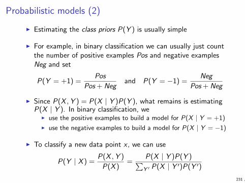
Probabilistic models (2)
I Estimating the class priors P(Y ) is usually simple
I For example, in binary classification we can usually just countthe number of positive examples Pos and negative examplesNeg and set
P(Y = +1) =Pos
Pos + Negand P(Y = −1) =
Neg
Pos + Neg
I Since P(X ,Y ) = P(X | Y )P(Y ), what remains is estimatingP(X | Y ). In binary classification, we
I use the positive examples to build a model for P(X | Y = +1)
I use the negative examples to build a model for P(X | Y = −1)
I To classify a new data point x , we can use
P(Y | X ) =P(X ,Y )
P(X )=
P(X | Y )P(Y )∑Y ′ P(X | Y ′)P(Y ′)
231 ,

Categorical features
I Assume we have d input features X1, . . . ,Xd where thepossible values for Xi are { 1, . . . , ri } for some (small) numberri of distinct values
I There are |X | =∏d
i=1 ri possible inputs we may need toclassify
I To determine an arbitrary distribution over X we would need|X | − 1 parameters (since probabilities sum to one but canotherwise be chosen freely to each x ∈ X )
I It would be clearly nonsensical to assume that all possiblex ∈ X are actually present in training data so we need to dosome simplifying assumptions
232 ,
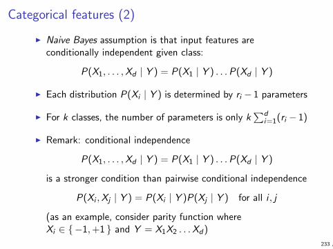
Categorical features (2)
I Naive Bayes assumption is that input features areconditionally independent given class:
P(X1, . . . ,Xd | Y ) = P(X1 | Y ) . . .P(Xd | Y )
I Each distribution P(Xi | Y ) is determined by ri − 1 parameters
I For k classes, the number of parameters is only k∑d
i=1(ri − 1)
I Remark: conditional independence
P(X1, . . . ,Xd | Y ) = P(X1 | Y ) . . .P(Xd | Y )
is a stronger condition than pairwise conditional independence
P(Xi ,Xj | Y ) = P(Xi | Y )P(Xj | Y ) for all i , j
(as an example, consider parity function whereXi ∈ {−1,+1 } and Y = X1X2 . . .Xd)
233 ,
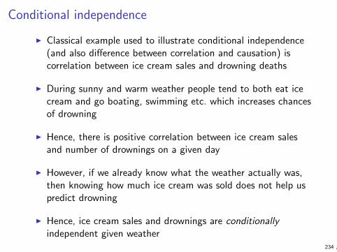
Conditional independence
I Classical example used to illustrate conditional independence(and also difference between correlation and causation) iscorrelation between ice cream sales and drowning deaths
I During sunny and warm weather people tend to both eat icecream and go boating, swimming etc. which increases chancesof drowning
I Hence, there is positive correlation between ice cream salesand number of drownings on a given day
I However, if we already know what the weather actually was,then knowing how much ice cream was sold does not help uspredict drowning
I Hence, ice cream sales and drownings are conditionallyindependent given weather
234 ,

Learning a naive Bayes model
I Assume there are k classes c1, . . . , ck and d input featureswhere for i = 1, . . . , d feature Xi has ranger(Xi ) = { 1, . . . , ri }
I We model P(X | Y = c) separately for each classc ∈ { c1, . . . , ck } and feature X ∈ {X1, . . . ,Xd }:
I For v ∈ r(X ), let nv be the number of examples in trainingdata that have class c and feature value Xi = v , andn =
∑v∈r(X ) nv
I We estimate
P(X = v | Y = c) =nv + mv
n + m
where mv is a pseudocount (see slide 168) and andm =
∑v mv
I Usual choices for pseudocounts are mv = 0 (empiricalprobabilities) and mv = 1 (Laplace correction)
235 ,
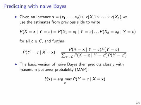
Predicting with naive Bayes
I Given an instance x = (x1, . . . , xd) ∈ r(X1)× · · · × r(Xd) weuse the estimates from previous slide to write
P(X = x | Y = c) = P(X1 = x1 | Y = c) . . .P(Xd = xd | Y = c)
for all c ∈ C , and further
P(Y = c | X = x) =P(X = x | Y = c)P(Y = c)∑
c ′∈C P(X = x | Y = c ′)P(Y = c ′)
I The basic version of naive Bayes then predicts class c withmaximum posterior probability (MAP):
c(x) = arg maxc
P(Y = c | X = x)
236 ,

Predicting with naive Bayes (2)
I Since the denominator∑
c ′∈C P(X = x | Y = c ′)P(Y = c ′)does not depend on c , this is the same as
c(x) = arg maxc
P(X = x | Y = c)P(Y = c)
I If the class prior P(Y ) is uniform, this simplifies to maximumlikelihood (ML) prediction
c(x) = arg maxc
P(X = x | Y = c)
237 ,

Predicting with naive Bayes (3)
I Textbook recommends the more sophisticated method ofchoosing
c(x) = arg maxc
wcP(X = x | Y = c)
where weights wc for each class are chosen to minimiseclassification error
I For binary classification this turns out to be same as rankingthe examples x according to likelihood ratio
P(X = x | Y = +1)
P(X = x | Y = −1)
and turning the ranker into classifier as discussed on slides116–117
I For three or more classes this becomes more complicated, andwe will not go into details
238 ,

About naive Bayes assumption
I The assumption that features are independent conditioned onclass is
I very strong
I often quite untrue
I Therefore in particular the probabilities produced by a naiveBayes model should not be trusted too much
I However the ranking and classification performance of naiveBayes are often quite good in practice
I One “justification” for using naive Bayes is that we conciouslyuse a model with high bias in order to reduce variance
I for example text classification: if we use one feature for eachword in our vocabulary, the number of features can easily bemuch larger than the number of training examples
239 ,
Representing documents
I We consider some special issues when instances consist ofdocuments written in (more or less) natural language
I We assume there is a vocabulary of d words w1, . . . ,wd thatmay occur in documents
I Instead of just single words, we may also consider pairs ofadjacent words, triples, etc.
I We have k classes c1, . . . , ck where k may be 2 (spamfiltering) or several hundreds (news article topics)
I Standard preprocessing techniques includeI stop words: ignore common words such as ‘have’, ‘the’ and ‘it’
that tell us little about the content of the document
I lemmatisation: recognise that e.g. ‘send’, ‘sent’ and ‘sending’are just different forms of the same word
240 ,

Boolean model for text
I In this model, we present a document by d binary featuresX1, . . . ,Xd where Xi = 1 if word wi occurs at least once inthe document, and Xi = 0 otherwise
I In naive Bayes model we assume the features Xi independentgiven class
I Hence, we estimate for each class c and word wi theprobability pc,i that document of class c contains word wi
(see slide 235 for estimating probabilities)
I Then for feature vector x = (x1, . . . , xd) ∈ { 0, 1 }d we have
P(x | Y = c) =d∏
i=1
pxic,i (1− pc,i )
1−xi
241 ,

Multinomial model for text
I In this model we represent a document with d numericalfeatures, where Xi ∈ { 0, 1, 2, . . . } is the number ofoccurences of word wi in the document (bag of words)
I In naive Bayes model we assume that first the total number ofwords N in a document is chosen, and then each of the N“slots” is filled independently with word wi being chosen withprobability pc,i for document in class c
I Notice that here∑d
i=1 pc,i = 1 for all classes c
I The probability of a frequency vector x = (x1, . . . , xd) ∈ Nd
with∑d
i=1 xi = n follows multinomial distribution
P(x | Y = c ,N = n) =n!
x1! . . . xd !px1c,1 . . . p
xdc,d
242 ,

Normal distribution
I For probabilistic models for real-valued features xi ∈ R, onebasic ingredient is the normal or Gaussian distribution
I Recall that for a single real-valued random variable, thenormal distribution has two parameters µ and σ2, and density
N (x | µ, σ2) =1√2πσ
exp
(−(x − µ)2
2σ2
)
I If X has this distribution, then E[X ] = µ and Var[X ] = σ2
I For multivariate case x ∈ Rd , we shall first consider the casewhere individual component xi has normal distribution withparameters µi and σ2
i and the components are independent:
p(x) = N (x1 | µ1, σ21) . . .N (xd | µd , σ2
d)
243 ,
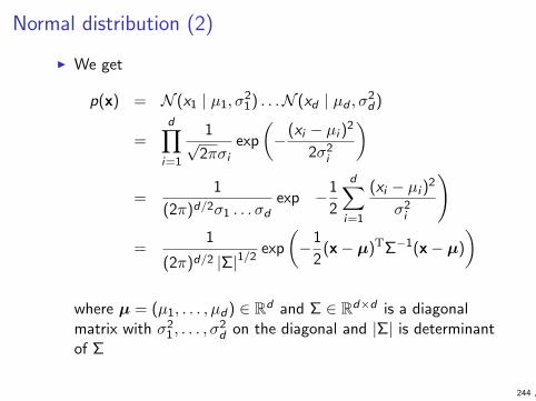
Normal distribution (2)
I We get
p(x) = N (x1 | µ1, σ21) . . .N (xd | µd , σ2
d)
=d∏
i=1
1√2πσi
exp
(−(xi − µi )2
2σ2i
)
=1
(2π)d/2σ1 . . . σdexp
(−1
2
d∑
i=1
(xi − µi )2
σ2i
)
=1
(2π)d/2 |Σ|1/2exp
(−1
2(x− µ)TΣ−1(x− µ)
)
where µ = (µ1, . . . , µd) ∈ Rd and Σ ∈ Rd×d is a diagonalmatrix with σ2
1, . . . , σ2d on the diagonal and |Σ| is determinant
of Σ
244 ,
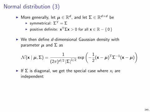
Normal distribution (3)
I More generally, let µ ∈ Rd , and let Σ ∈ Rd×d beI symmetrical: ΣT = Σ
I positive definite: xTΣx > 0 for all x ∈ R− { 0 }
I We then define d-dimensional Gaussian density withparameter µ and Σ as
N (x | µ,Σ) =1
(2π)d/2 |Σ|1/2exp
(−1
2(x− µ)TΣ−1(x− µ)
)
I If Σ is diagonal, we get the special case where xi areindependent
245 ,
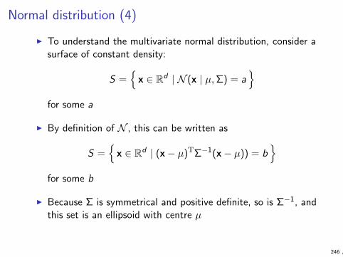
Normal distribution (4)
I To understand the multivariate normal distribution, consider asurface of constant density:
S ={x ∈ Rd | N (x | µ,Σ) = a
}
for some a
I By definition of N , this can be written as
S ={x ∈ Rd | (x− µ)TΣ−1(x− µ)) = b
}
for some b
I Because Σ is symmetrical and positive definite, so is Σ−1, andthis set is an ellipsoid with centre µ
246 ,
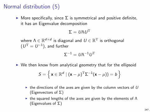
Normal distribution (5)
I More specifically, since Σ is symmetrical and positive definite,it has an Eigenvalue decomposition
Σ = UΛUT
where Λ ∈ Rd×d is diagonal and U ∈ RT is orthogonal(UT = U−1), and further
Σ−1 = UΛ−1UT
I We then know from analytical geometry that for the ellipsoid
S ={x ∈ Rd | (x− µ)TΣ−1(x− µ)) = b
}
I the directions of the axes are given by the column vectors of U(Eigenvectors of Σ)
I the squared lengths of the axes are given by the elements of Λ(Eigenvalues of Σ)
247 ,

Normal distribution (6)
I Let X = (X1, . . . ,Xd) have normal distribution withparameters µ and Σ
I Then E[X] = µ and E[(Xi − µi )(Xj − µj)] = Σij
I Hence, we call the parameter µ the mean and Σ thecovariance matrix
248 ,

Normal distribution (7)
I Let x1, . . . , xn be independent samples from a normaldistribution with unknown mean µ and covariance Σ
I The maximum likelihood estimates
(µ, Σ) = arg maxµ,Σ
n∏
i=1
N (xi | µ,Σ)
are given by
µp =1
n
n∑
i=1
xi ,p
Σpq =1
n
n∑
i=1
(xi ,p − µp)(xi ,q − µq)
where we write xi = (xi ,1, . . . , xi ,d) etc.
249 ,
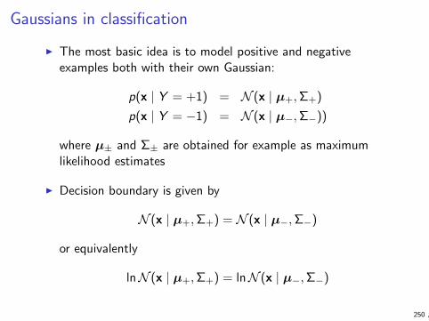
Gaussians in classification
I The most basic idea is to model positive and negativeexamples both with their own Gaussian:
p(x | Y = +1) = N (x | µ+,Σ+)
p(x | Y = −1) = N (x | µ−,Σ−))
where µ± and Σ± are obtained for example as maximumlikelihood estimates
I Decision boundary is given by
N (x | µ+,Σ+) = N (x | µ−,Σ−)
or equivalently
lnN (x | µ+,Σ+) = lnN (x | µ−,Σ−)
250 ,

Gaussians in classification (2)
I By substituting the formula for N into
lnN (x | µ+,Σ+) = lnN (x | µ−,Σ−)
and simplifying we get
(x−µ+)TΣ−1+ (x−µ+)−(x−µ−)TΣ−1
− (x−µ−)+ln|Σ−||Σ+|
= 0
I If Σ+ = Σ− this is a linear equation, so the decision boundaryis a hyperplane
I In general case this is a quadratic surface and decision regionsmay be non-connected (as we saw earlier in one-dimensionalcase)
251 ,
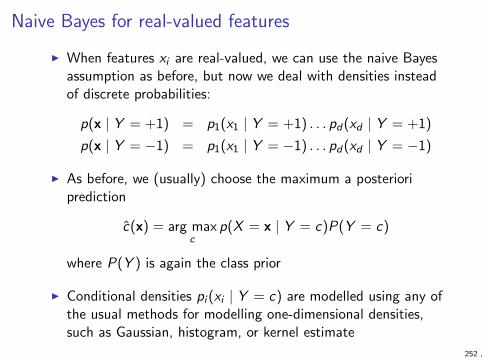
Naive Bayes for real-valued features
I When features xi are real-valued, we can use the naive Bayesassumption as before, but now we deal with densities insteadof discrete probabilities:
p(x | Y = +1) = p1(x1 | Y = +1) . . . pd(xd | Y = +1)
p(x | Y = −1) = p1(x1 | Y = −1) . . . pd(xd | Y = −1)
I As before, we (usually) choose the maximum a posterioriprediction
c(x) = arg maxc
p(X = x | Y = c)P(Y = c)
where P(Y ) is again the class prior
I Conditional densities pi (xi | Y = c) are modelled using any ofthe usual methods for modelling one-dimensional densities,such as Gaussian, histogram, or kernel estimate
252 ,
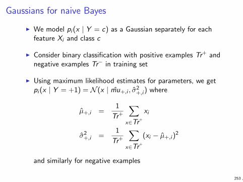
Gaussians for naive Bayes
I We model pi (x | Y = c) as a Gaussian separately for eachfeature Xi and class c
I Consider binary classification with positive examples Tr+ andnegative examples Tr− in training set
I Using maximum likelihood estimates for parameters, we getpi (x | Y = +1) = N (x | mu+,i , σ
2+,i ) where
µ+,i =1
Tr+
∑
x∈Tr+
xi
σ2+,i =
1
Tr+
∑
x∈Tr+
(xi − µ+,i )2
and similarly for negative examples
253 ,

Density estimate by histogram
I Histograms are a non-parametric method for estimatingone-dimensional density
I Assume for simplicity that all data points in sample are inrange [0,M)
I Divide the range into k intervals I1, . . . , Ik of length ∆ where∆ = M/k and Ii = [(i − 1)∆, i∆)
I Let ni be the number of data points in the sample that belongto interval Ii , and n =
∑i ni the sample size
I Histogram estimate is a piecewise constant density
p(x) =1
∆
ni
nwhen x ∈ Ii
254 ,

Kernel density estimation
I Kernel density estimation is another non-parametric method
I We choose a kernel width parameter σI large σ gives smoother estimate with less detail
I Given data points x1, . . . , xn, we put a Gaussian with varianceσ2 on top of each of them, and add the distributions togetherwith proper normalisation:
p(x) =1
n
n∑
i=1
N (x | xi , σ2)
255 ,

Logistic regression
I Logistic regression models are linear models for probabilisticbinary classification (so, not really regression)
I We calculate score s(x) for x ∈ Rd as
s(x) = w · x− t
where parameters w ∈ Rd and t ∈ R are learned from data
I Scores are converted to probabilitiesp(x) = P(Y = 1 | X = x) using logistic sigmoid
p(x) =1
1 + exp(−s(x))
I This is a discriminative probabilitic model: we model onlyP(Y | X ), not P(X )
256 ,
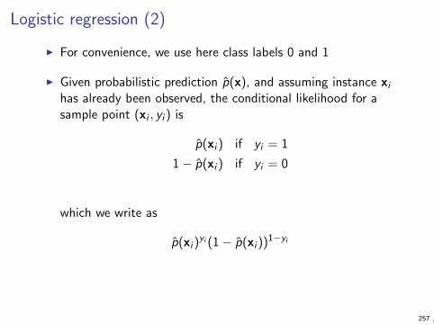
Logistic regression (2)
I For convenience, we use here class labels 0 and 1
I Given probabilistic prediction p(x), and assuming instance xihas already been observed, the conditional likelihood for asample point (xi , yi ) is
p(xi ) if yi = 1
1− p(xi ) if yi = 0
which we write as
p(xi )yi (1− p(xi ))1−yi
257 ,

Logistic regression (3)
I Conditional likelihood of sequence of independent samples(xi , yi ), i = 1, . . . , n is then
∏ni=1 p(xi )
yi (1− p(xi ))1−yi
I we say ‘conditional’ to emphasise that we take xi as given andonly model probability of labels yi
I To maximise conditional likelihood, we can equivalentlymaximise conditional log-likelihood
LCL(w, t)) = lnn∏
i=1
p(xi )yi (1− p(xi )
1−yi )
=n∑
i=1
(yi ln p(xi ) + (1− yi ) ln(1− p(xi )))
I Notice that this is the same as minimising logaritmic cost(slide 96)
258 ,
Logistic regression (4)
I Logistic regression is a case of Generalized Linear Models(GLM)
I Optimisation tools exist and are included in many standardpackages
I Often used with regularisation, as in linear regressionI “ridge”: arg max(LCL(w, t)− λ ‖w‖2
2)
I “lasso”: arg max(LCL(w, t)− λ ‖w‖1)
I In particular, if data is linearly separable, non-regularisedsolution tends to infinity
259 ,

Probabilistic models: summary
I Generative probabilistic models often involve modellingP(X | Y = c) for different classes c
I Important tools for this includeI multivariate Gaussians: very important overall in statistics and
machine learning, important to be familiar with them
I naive Bayes assumption: commonly used in practice, importantto understand its uses and limitations
I We also saw logistic regression as example of discriminativeprobabilistic model
260 ,

Probabilistic models in textbook
I We more or less covered all of Sections 9.0, 9.1, 9.2 and 9.3,although in some places we tried to give the intuition from aslightly different point of view
I you are not required to read the mathematical derivations onpp. 272–273 and 284–285, although they are not toocomplicated and understanding them should be helpful
I you may also omit discussion on calibration, which is atechnique from earlier in the textbook that we skipped
I Section 9.4 is beyond the scope of this course, but the topics(latent variables and EM algorithm) are very important if youget any deeper into machine learning
I Minimum Description Length from Section 9.5 is covered incourse Information Theoretic Modeling
261 ,

Clustering
262 ,

Partitional clustering: basic idea
I Each data vector xi is assigned to one of K clusters
I Typically K and a similarity measure is selected by the user,while the chosen algorithm then learns the actual partition
I In the example below, K = 3 and the partition are shownusing color (red, green, blue)
X X
⇒
263 ,

Partitional clustering: basic idea (2)
I Intuitively, in a good partitional clusteringI data points in same cluster are similar (close) to each other
I data points in different clusters are dissimilar (distant) fromeach other
I Partitional clustering is often represented by giving Kexemplars (or prototypes) µ1, . . . ,µK and assigning each datapoint to the closest exemplar
I This makes the clustering predictive: if we observe a new datapoint, our clustering model can directly assign it to a cluster
I The textbook does not use term “partitional clustering,” butin practice partitional clustering methods largely coincide withdistance-based clustering methods presented in the textbook
264 ,
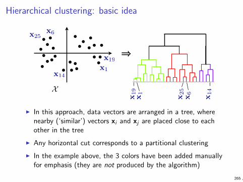
Hierarchical clustering: basic idea
X
⇒x1
x14
x25x6
x19
x1
x19
x25
x6
x14
I In this approach, data vectors are arranged in a tree, wherenearby (‘similar’) vectors xi and xj are placed close to eachother in the tree
I Any horizontal cut corresponds to a partitional clustering
I In the example above, the 3 colors have been added manuallyfor emphasis (they are not produced by the algorithm)
265 ,

Motivation for clustering
Understanding the data:
I Information retrieval:
organizing a set of documents for easy browsing (for example ahierarchical structure to the documents)
266 ,
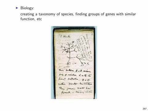
I Biology:
creating a taxonomy of species, finding groups of genes with similarfunction, etc
267 ,

I Medicine:
understanding the relations among diseases or psychologicalconditions, to aid in discovering the most useful treatments
522 14. Unsupervised Learning
4060
80100
CNS
CNS
CNS
RENA
L
BREA
ST
CNSCN
S
BREA
ST
NSCL
C
NSCL
C
RENA
LRE
NAL
RENA
LRENA
LRE
NAL
RENA
L
RENA
L
BREA
STNS
CLC
RENA
L
UNKN
OWN
OVA
RIAN
MELAN
OMA
PROST
ATEOVA
RIAN
OVA
RIAN
OVA
RIAN
OVA
RIAN
OVA
RIAN
PROST
ATE
NSCL
CNS
CLC
NSCL
C
LEUK
EMIA
K562B-repro
K562A-repro
LEUK
EMIA
LEUK
EMIA
LEUK
EMIA
LEUK
EMIA
LEUK
EMIA
COLO
NCO
LON
COLO
NCO
LON
COLO
N
COLO
NCO
LON
MCF
7A-repro
BREA
STMCF
7D-repro
BREA
ST
NSCL
C
NSCL
CNS
CLC
MELAN
OMA
BREA
STBR
EAST
MELAN
OMA
MELAN
OMA
MELAN
OMA
MELAN
OMA
MELAN
OMA
MELAN
OMA
FIGURE 14.12. Dendrogram from agglomerative hierarchical clustering withaverage linkage to the human tumor microarray data.
chical structure produced by the algorithm. Hierarchical methods imposehierarchical structure whether or not such structure actually exists in thedata.
The extent to which the hierarchical structure produced by a dendro-gram actually represents the data itself can be judged by the copheneticcorrelation coefficient. This is the correlation between the N(N −1)/2 pair-wise observation dissimilarities dii′ input to the algorithm and their corre-sponding cophenetic dissimilarities Cii′ derived from the dendrogram. Thecophenetic dissimilarity Cii′ between two observations (i, i′) is the inter-group dissimilarity at which observations i and i′ are first joined togetherin the same cluster.
The cophenetic dissimilarity is a very restrictive dissimilarity measure.First, the Cii′ over the observations must contain many ties, since only N−1of the total N(N − 1)/2 values can be distinct. Also these dissimilaritiesobey the ultrametric inequality
Cii′ ≤ max{Cik, Ci′k} (14.40)
268 ,

I Business:
grouping customers by their preferences or shopping behavior, forinstance for targeted advertisement campaigns
For example:
I Customers who follow advertisements carefully, and when inthe shop buy only what is on sale
I Customers who do not seem to react to advertisements at all
I Customers who are attracted by advertisements, also buy otherthings in the store while there...
To whom should you send advertisements?
269 ,

I Other motivations: simplifying the data for furtherprocessing/transmission
I Summarization:
reduce the effective amount of data by considering only theexemplars rather than the original data vectors
I ‘Lossy’ compression:
saving disk space by only storing a exemplar vector which is‘close enough’
270 ,

Distance-based clustering
I We are given a data set D = { x1, . . . , xn } ⊂ X and a notionof similarity between elements of X
I The output will be a partition (D1, . . . ,DK ) of D:I D1 ∪ · · · ∪ DK = D
I Di ∩ Dj = ∅ if i 6= j
I Alternatively, we can represent the partition by giving anassignment mapping where j(i) = p if xi ∈ Dp
I We usually also output K exemplars µ1, . . . ,µK where eachdata point is assigned to the cluster with closest exemplar
I number of clusters K is usually given as input; choosing a“good” K is a separate (non-trivial) issue
271 ,
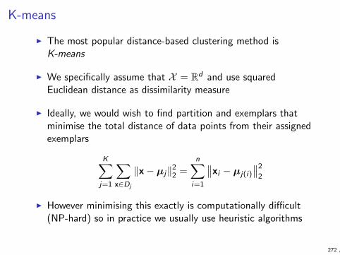
K-means
I The most popular distance-based clustering method isK-means
I We specifically assume that X = Rd and use squaredEuclidean distance as dissimilarity measure
I Ideally, we would wish to find partition and exemplars thatminimise the total distance of data points from their assignedexemplars
K∑
j=1
∑
x∈Dj
‖x− µj‖22 =
n∑
i=1
∥∥xi − µj(i)
∥∥2
2
I However minimising this exactly is computationally difficult(NP-hard) so in practice we usually use heuristic algorithms
272 ,
Hard vs. soft clustering
I In soft clustering we assign to each pair xi and Dj a number
rij ∈ [0, 1] so that∑K
j=1 rij = 1 for all i , and then minimise
n∑
i=1
K∑
j=1
rij ‖xi − µj‖22
I Hard clustering, which we discuss here, is the special casewhere we require that for each i there is exactly one j(i) suchthat ri ,j(i) = 1, and rij = 0 for j 6= j(i)
I Soft clustering can be approached for example using theExpectation-Maximisation (EM) algorithm, which is beyondthe scope of our course (but discussed in Section 9.4 oftextbook)
273 ,
K-means algorithm
I We start by picking K initial cluster exemplars (for examplerandomly from our data set)
I We then alternate between the following two steps, untilnothing changes any more:
I Keeping the examplars fixed, assign each data point to theclosest exemplar
I Keeping the assignments fixed, move each exemplar to thecenter of its assigned data points
I In this context we call the exemplars cluster means. Noticethat generally they are not sample points in our data set, butcan be arbitrary vectors in Rd
I This is also known as Lloyd’s algorithm; see Algorithm 8.1 intextbook
274 ,
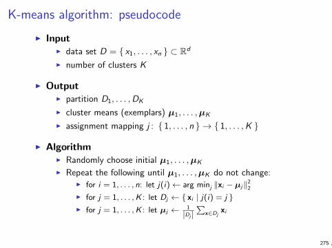
K-means algorithm: pseudocode
I InputI data set D = { x1, . . . , xn } ⊂ Rd
I number of clusters K
I OutputI partition D1, . . . ,DK
I cluster means (exemplars) µ1, . . . ,µK
I assignment mapping j : { 1, . . . , n } → { 1, . . . ,K }
I AlgorithmI Randomly choose initial µ1, . . . ,µK
I Repeat the following until µ1, . . . ,µK do not change:I for i = 1, . . . , n: let j(i)← arg minj ‖xi − µj‖2
2
I for j = 1, . . . ,K : let Dj ← { xi | j(i) = j }I for j = 1, . . . ,K : let µj ← 1
|Dj |∑
x∈Djxi
275 ,

K-means: 2D example
(a)
!2 0 2
!2
0
2 (b)
!2 0 2
!2
0
2 (c)
!2 0 2
!2
0
2 (d)
!2 0 2
!2
0
2 (e)
!2 0 2
!2
0
2 (f)
!2 0 2
!2
0
2
�(a)
!2 0 2
!2
0
2 (b)
!2 0 2
!2
0
2 (c)
!2 0 2
!2
0
2 (d)
!2 0 2
!2
0
2 (e)
!2 0 2
!2
0
2 (f)
!2 0 2
!2
0
2
� I Data from the ‘Old faithful’ geyser (horizontal axis is durationof eruption, vertical axis is waiting time to the next eruption,both scaled to zero mean and unit variance)
276 ,

K-means: convergence
I We can show that the algorithm is guaranteed to convergeafter some finite number of steps
I We look into changes of the cost function
Cost =K∑
j=1
∑
x∈Dj
‖x− µj‖22 =
n∑
i=1
∥∥xi − µj(i)
∥∥2
2
at the two steps inside the main loop
I In first step, we assign each xi to j(i) such that∥∥xi − µj(i)
∥∥2
2is minimised
I In second step, we choose each µj as the mean of Dj , which
minimises∑
x∈Dj‖x− µj‖2
2 for a fixed Dj
I This is essentially shown in Homework 6, problem 3(a)
I Hence, the cost never increases
277 ,

K-means: convergence (2)
I There is a finite number Kn possible assignments, so there isonly a finite number of possible values for Cost
I Since Cost is non-increasing, it must eventually stabilise toone value
I Notice that the value to which we convergeI is not guaranteed to be global optimum of Cost
I depends on initialisation of cluster means
I In practice, convergence usually takes a lot fewer than Kn
steps
278 ,
Space and time complexity
I Space requirements are modest, as (in addition to the dataitself) we only need to store:
1. The index of the assigned cluster for each datapoint xi
2. The cluster centroid for each cluster
I The running time is linear in all the relevant parameters, i.e.O(MnKd), where M is the number of iterations, n thenumber of samples, K the number of clusters, and d thenumber of dimensions (attributes).
(The number of iterations M typically does not depend heavily on
the other parameters.)
279 ,
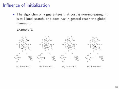
Influence of initialization
I The algorithm only guarantees that cost is non-increasing. Itis still local search, and does not in general reach the globalminimum.
Example 1: 8.2 K-means 503
(a) Iteration 1. (b) Iteration 2. (c) Iteration 3. (d) Iteration 4.
Figure 8.5. Poor starting centroids for K-means.
cluster, the centroids will redistribute themselves so that the “true” clustersare found. However, Figure 8.7 shows that if a pair of clusters has only oneinitial centroid and the other pair has three, then two of the true clusters willbe combined and one true cluster will be split.
Note that an optimal clustering will be obtained as long as two initialcentroids fall anywhere in a pair of clusters, since the centroids will redistributethemselves, one to each cluster. Unfortunately, as the number of clustersbecomes larger, it is increasingly likely that at least one pair of clusters willhave only one initial centroid. (See Exercise 4 on page 559.) In this case,because the pairs of clusters are farther apart than clusters within a pair, theK-means algorithm will not redistribute the centroids between pairs of clusters,and thus, only a local minimum will be achieved.
Because of the problems with using randomly selected initial centroids,which even repeated runs may not overcome, other techniques are often em-ployed for initialization. One effective approach is to take a sample of pointsand cluster them using a hierarchical clustering technique. K clusters are ex-tracted from the hierarchical clustering, and the centroids of those clusters areused as the initial centroids. This approach often works well, but is practicalonly if (1) the sample is relatively small, e.g., a few hundred to a few thousand(hierarchical clustering is expensive), and (2) K is relatively small comparedto the sample size.
The following procedure is another approach to selecting initial centroids.Select the first point at random or take the centroid of all points. Then, foreach successive initial centroid, select the point that is farthest from any ofthe initial centroids already selected. In this way, we obtain a set of initial
280 ,

Example 2: 8.2 K-means 505
(a) Iteration 1. (b) Iteration 2.
(c) Iteration 3. (d) Iteration 4.
Figure 8.7. Two pairs of clusters with more or fewer than two initial centroids within a pair of clusters.
is less susceptible to initialization problems (bisecting K-means) and usingpostprocessing to “fixup” the set of clusters produced.
Time and Space Complexity
The space requirements for K-means are modest because only the data pointsand centroids are stored. Specifically, the storage required is O((m + K)n),where m is the number of points and n is the number of attributes. The timerequirements for K-means are also modest—basically linear in the number ofdata points. In particular, the time required is O(I ∗K ∗m∗n), where I is thenumber of iterations required for convergence. As mentioned, I is often smalland can usually be safely bounded, as most changes typically occur in the
I One possible solution: Run the algorithm from many randominitial conditions, select the end result with the smallest cost.(Nevertheless, it may still find very ‘bad’ solutions almost allthe time.)
281 ,

How to select the number of clusters?
I Not a priori clear what the ‘optimal’ number of clusters is:8.1 Overview 491
(a) Original points. (b) Two clusters.
(c) Four clusters. (d) Six clusters.
Figure 8.1. Different ways of clustering the same set of points.
in the sense of Chapter 4 is supervised classification; i.e., new, unlabeledobjects are assigned a class label using a model developed from objects withknown class labels. For this reason, cluster analysis is sometimes referredto as unsupervised classification. When the term classification is usedwithout any qualification within data mining, it typically refers to supervisedclassification.
Also, while the terms segmentation and partitioning are sometimesused as synonyms for clustering, these terms are frequently used for approachesoutside the traditional bounds of cluster analysis. For example, the termpartitioning is often used in connection with techniques that divide graphs intosubgraphs and that are not strongly connected to clustering. Segmentationoften refers to the division of data into groups using simple techniques; e.g.,an image can be split into segments based only on pixel intensity and color, orpeople can be divided into groups based on their income. Nonetheless, somework in graph partitioning and in image and market segmentation is relatedto cluster analysis.
8.1.2 Different Types of Clusterings
An entire collection of clusters is commonly referred to as a clustering, and inthis section, we distinguish various types of clusterings: hierarchical (nested)versus partitional (unnested), exclusive versus overlapping versus fuzzy, andcomplete versus partial.
Hierarchical versus Partitional The most commonly discussed distinc-tion among different types of clusterings is whether the set of clusters is nested
I The more clusters, the lower the cost, so need some form of‘model selection’ approach
I Will discuss this a bit more in the context of clusteringvalidation strategies later
282 ,
Variants of K-means
I In basic K-means, we always choose cluster means asexemplars:
µj ←1
|Dj |∑
x∈Dj
xi
I An alternative is to pick one of the data points in the clusteras exemplar:
µj ← arg minx∈Dj
∑
x′∈Dj
Dis(x, x′)
where Dis is now an arbitrary measure of dissimilarity
I We do not even need the instance space to be Rd
I This is known as K-medoids (Algorithm 8.2 in textbook), andthe exemplar as medoids
283 ,
Variants of K-means (2)
I We can refine the search for good medoids (Algorithm 8.3):I Define cost function
K∑
j=1
∑
x∈Dj
Dis(x,µj)
I Consider each cluster j and current non-medoidx ∈ D − {µ1, . . . ,µK } and calculate change in cost if wechange µj ← x
I Do the change µj ← x that leads to lowest cost
I Time requirement for a single update is O(n2)I O(n) for single evaluation of cost
I k(n − k) pairs (x, j) to consider
I Convergence in finite number of iterations can be proven aswith basic K-means
284 ,

Evaluating clustering quality
I Suppose we have created a clustering with examplarsµ1, . . . ,µK
I Suppose further that we have m data points z1, . . . , zm suchthat for each pair (zi , zj) we know from some source whetherthey should be grouped together or not
I We use this to create a binary classification data set of sizem(m − 1)/2 consisting of ((zi , zj), cij) where cij = +1 if ziand zj belong together
I We then interpret our clustering as classifier c for pairs (z, z′)where c(z, z′) = +1 if
arg minj
Dis(z,µj) = arg minj
Dis(z′,µj)
285 ,

I We can then evaluate the clustering like we would evaluateany binary classifier on a test set
I However we generally expect there to be a lot fewer positiveexamples (pairs that belong together) than negative examples,so classification accuracy may not be a good measure
I A popular choice is F-measure which is defined as harmonicaverage of precision and recall:
1
F=
1
2
(1
prec+
1
rec
)⇒
F =2prec · rec
prec + rec
286 ,
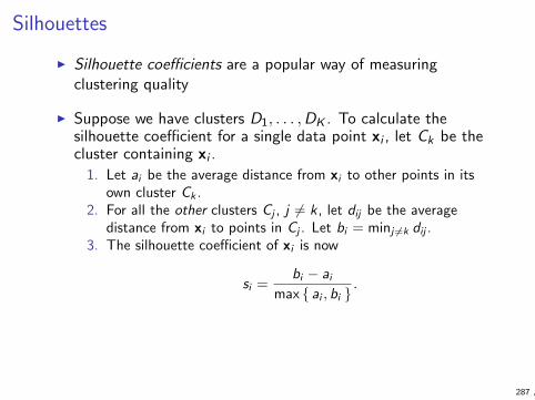
Silhouettes
I Silhouette coefficients are a popular way of measuringclustering quality
I Suppose we have clusters D1, . . . ,DK . To calculate thesilhouette coefficient for a single data point xi , let Ck be thecluster containing xi .
1. Let ai be the average distance from xi to other points in itsown cluster Ck .
2. For all the other clusters Cj , j 6= k , let dij be the averagedistance from xi to points in Cj . Let bi = minj 6=k dij .
3. The silhouette coefficient of xi is now
si =bi − ai
max { ai , bi }.
287 ,

Silhouettes (2)
I The silhoutte coefficient varies in range [−1, 1].
I Negative value of si means that xi is on the average actuallycloser to points in some other cluster than its own.
I One can use the average of silhouette coefficients in a singlecluster as an indication of goodness of that cluster.
I One can also use the average of silhouette coefficients over allthe data points as an indication of goodness of the wholeclustering.
I The actual numerical values of silhouette coefficients areprobably hard to interpret, but they can be helpful incomparing different ways of clustering the same data.
I Which clustering algorithm is better?
I What’s a good number of clusters?
288 ,
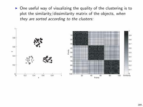
I One useful way of visualizing the quality of the clustering is toplot the similarity/dissimilarity matrix of the objects, whenthey are sorted according to the clusters:544 Chapter 8 Cluster Analysis: Basic Concepts and Algorithms
0 0.2 0.4 0.6 0.8 10
0.2
0.4
0.6
0.8
1
x
y
(a) Well-separated clusters.
Points
Po
ints
20 40 60 80 100
10
20
30
40
50
60
70
80
90
100Similarity
0
1
0.9
0.8
0.7
0.6
0.5
0.4
0.3
0.2
0.1
(b) Similarity matrix sorted by K-meanscluster labels.
Figure 8.30. Similarity matrix for well-separated clusters.
The well-separated clusters in Figure 8.30 show a very strong, block-diagonal pattern in the reordered similarity matrix. However, there are alsoweak block diagonal patterns—see Figure 8.31—in the reordered similaritymatrices of the clusterings found by K-means, DBSCAN, and complete linkin the random data. Just as people can find patterns in clouds, data miningalgorithms can find clusters in random data. While it is entertaining to findpatterns in clouds, it is pointless and perhaps embarrassing to find clusters innoise.
This approach may seem hopelessly expensive for large data sets, sincethe computation of the proximity matrix takes O(m2) time, where m is thenumber of objects, but with sampling, this method can still be used. We cantake a sample of data points from each cluster, compute the similarity betweenthese points, and plot the result. It may be necessary to oversample smallclusters and undersample large ones to obtain an adequate representation ofall clusters.
8.5.4 Unsupervised Evaluation of Hierarchical Clustering
The previous approaches to cluster evaluation are intended for partitionalclusterings. Here we discuss the cophenetic correlation, a popular evaluationmeasure for hierarchical clusterings. The cophenetic distance between twoobjects is the proximity at which an agglomerative hierarchical clustering tech-
289 ,

I Often, the main interest is whether the found cluster structureis a feature of the population, of which our data vectors onlyconstitute a small sample. In this case, we can use resamplingtechniques to investigate.
For instance (if we have lots of data):
I Divide the data into L random subsamples
I Run the clustering algorithm on each subsample separately
I Compare the results. Any reliable structure in the data shouldshow up (almost) every time.
290 ,
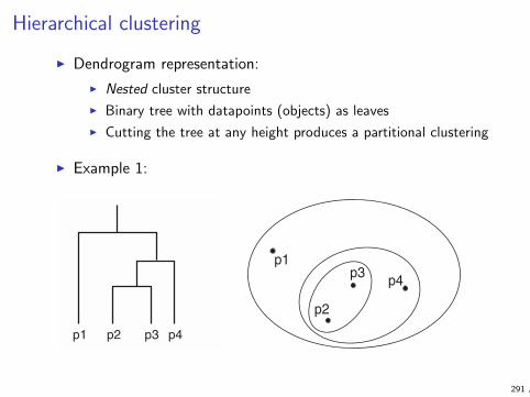
Hierarchical clustering
I Dendrogram representation:
I Nested cluster structure
I Binary tree with datapoints (objects) as leaves
I Cutting the tree at any height produces a partitional clustering
I Example 1:516 Chapter 8 Cluster Analysis: Basic Concepts and Algorithms
p1 p2 p3 p4
(a) Dendrogram.
p1
p2
p3p4
(b) Nested cluster diagram.
Figure 8.13. A hierarchical clustering of four points shown as a dendrogram and as nested clusters.
relationships and the order in which the clusters were merged (agglomerativeview) or split (divisive view). For sets of two-dimensional points, such as thosethat we will use as examples, a hierarchical clustering can also be graphicallyrepresented using a nested cluster diagram. Figure 8.13 shows an example ofthese two types of figures for a set of four two-dimensional points. These pointswere clustered using the single-link technique that is described in Section 8.3.2.
8.3.1 Basic Agglomerative Hierarchical Clustering Algorithm
Many agglomerative hierarchical clustering techniques are variations on a sin-gle approach: starting with individual points as clusters, successively mergethe two closest clusters until only one cluster remains. This approach is ex-pressed more formally in Algorithm 8.3.
Algorithm 8.3 Basic agglomerative hierarchical clustering algorithm.
1: Compute the proximity matrix, if necessary.2: repeat3: Merge the closest two clusters.4: Update the proximity matrix to reflect the proximity between the new
cluster and the original clusters.5: until Only one cluster remains.
291 ,

I Example 2:8.3 Agglomerative Hierarchical Clustering 521
6
4
52
1
33
2
4
5
1
(a) Complete link clustering.
0.4
0.3
0.2
0.1
03 6 4 1 2 5
(b) Complete link dendrogram.
Figure 8.17. Complete link clustering of the six points shown in Figure 8.15.
are merged first. However, {3, 6} is merged with {4}, instead of {2, 5} or {1}because
dist({3, 6}, {4}) = max(dist(3, 4), dist(6, 4))
= max(0.15, 0.22)
= 0.22.
dist({3, 6}, {2, 5}) = max(dist(3, 2), dist(6, 2), dist(3, 5), dist(6, 5))
= max(0.15, 0.25, 0.28, 0.39)
= 0.39.
dist({3, 6}, {1}) = max(dist(3, 1), dist(6, 1))
= max(0.22, 0.23)
= 0.23.
Group Average
For the group average version of hierarchical clustering, the proximity of twoclusters is defined as the average pairwise proximity among all pairs of pointsin the different clusters. This is an intermediate approach between the singleand complete link approaches. Thus, for group average, the cluster proxim-
I Height of horizontal connectors indicate the dissimilaritybetween the combined clusters (details a bit later)
292 ,

General approaches to hierarchical clustering:
I Divisive approach:
1. Start with one cluster containing all the datapoints.
2. Repeat for all non-singleton clusters:
I Split the cluster in two using some partitional clusteringapproach (e.g. K-means)
I Agglomerative approach:
1. Start with each datapoint being its own cluster
2. Repeat until there is just one cluster left:
I Select the pair of clusters which are most similar and jointhem into a single cluster
(The agglomerative approach is much more common, and we willexclusively focus on it in what follows.)
293 ,

Linkage functions
I Agglomerative hierarchical clustering requires comparingsimilarities between pairs clusters, not just pairs of points
I There are different linkage functions that generalise a notionof dissimilarity Dis(x, y) between two points to apply to anytwo sets of points A and B:
I single linkage Lsingle(A,B)
I complete linkage Lcomplete(A,B)
I average linkage Laverage(A,B)
I centroid linkage Lcentroid(A,B)
294 ,
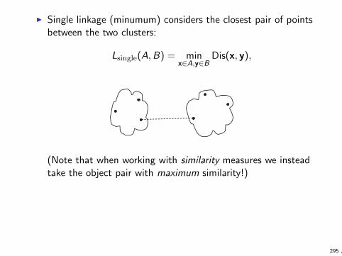
I Single linkage (minumum) considers the closest pair of pointsbetween the two clusters:
Lsingle(A,B) = minx∈A,y∈B
Dis(x, y),
8.3 Agglomerative Hierarchical Clustering 517
Defining Proximity between Clusters
The key operation of Algorithm 8.3 is the computation of the proximity be-tween two clusters, and it is the definition of cluster proximity that differ-entiates the various agglomerative hierarchical techniques that we will dis-cuss. Cluster proximity is typically defined with a particular type of clusterin mind—see Section 8.1.2. For example, many agglomerative hierarchicalclustering techniques, such as MIN, MAX, and Group Average, come froma graph-based view of clusters. MIN defines cluster proximity as the prox-imity between the closest two points that are in different clusters, or usinggraph terms, the shortest edge between two nodes in different subsets of nodes.This yields contiguity-based clusters as shown in Figure 8.2(c). Alternatively,MAX takes the proximity between the farthest two points in different clustersto be the cluster proximity, or using graph terms, the longest edge betweentwo nodes in different subsets of nodes. (If our proximities are distances, thenthe names, MIN and MAX, are short and suggestive. For similarities, however,where higher values indicate closer points, the names seem reversed. For thatreason, we usually prefer to use the alternative names, single link and com-plete link, respectively.) Another graph-based approach, the group averagetechnique, defines cluster proximity to be the average pairwise proximities (av-erage length of edges) of all pairs of points from different clusters. Figure 8.14illustrates these three approaches.
(a) MIN (single link.) (b) MAX (complete link.) (c) Group average.
Figure 8.14. Graph-based definitions of cluster proximity
If, instead, we take a prototype-based view, in which each cluster is repre-sented by a centroid, different definitions of cluster proximity are more natural.When using centroids, the cluster proximity is commonly defined as the prox-imity between cluster centroids. An alternative technique, Ward’s method,also assumes that a cluster is represented by its centroid, but it measures theproximity between two clusters in terms of the increase in the SSE that re-
(Note that when working with similarity measures we insteadtake the object pair with maximum similarity!)
295 ,
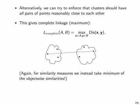
I Alternatively, we can try to enforce that clusters should haveall pairs of points reasonably close to each other
I This gives complete linkage (maximum):
Lcomplete(A,B) = maxx∈A,y∈B
Dis(x, y),
8.3 Agglomerative Hierarchical Clustering 517
Defining Proximity between Clusters
The key operation of Algorithm 8.3 is the computation of the proximity be-tween two clusters, and it is the definition of cluster proximity that differ-entiates the various agglomerative hierarchical techniques that we will dis-cuss. Cluster proximity is typically defined with a particular type of clusterin mind—see Section 8.1.2. For example, many agglomerative hierarchicalclustering techniques, such as MIN, MAX, and Group Average, come froma graph-based view of clusters. MIN defines cluster proximity as the prox-imity between the closest two points that are in different clusters, or usinggraph terms, the shortest edge between two nodes in different subsets of nodes.This yields contiguity-based clusters as shown in Figure 8.2(c). Alternatively,MAX takes the proximity between the farthest two points in different clustersto be the cluster proximity, or using graph terms, the longest edge betweentwo nodes in different subsets of nodes. (If our proximities are distances, thenthe names, MIN and MAX, are short and suggestive. For similarities, however,where higher values indicate closer points, the names seem reversed. For thatreason, we usually prefer to use the alternative names, single link and com-plete link, respectively.) Another graph-based approach, the group averagetechnique, defines cluster proximity to be the average pairwise proximities (av-erage length of edges) of all pairs of points from different clusters. Figure 8.14illustrates these three approaches.
(a) MIN (single link.) (b) MAX (complete link.) (c) Group average.
Figure 8.14. Graph-based definitions of cluster proximity
If, instead, we take a prototype-based view, in which each cluster is repre-sented by a centroid, different definitions of cluster proximity are more natural.When using centroids, the cluster proximity is commonly defined as the prox-imity between cluster centroids. An alternative technique, Ward’s method,also assumes that a cluster is represented by its centroid, but it measures theproximity between two clusters in terms of the increase in the SSE that re-
(Again, for similarity measures we instead take minimum ofthe objectwise similarities!)
296 ,
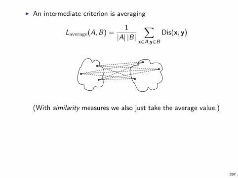
I An intermediate criterion is averaging
Laverage(A,B) =1
|A| |B|∑
x∈A,y∈BDis(x, y)
8.3 Agglomerative Hierarchical Clustering 517
Defining Proximity between Clusters
The key operation of Algorithm 8.3 is the computation of the proximity be-tween two clusters, and it is the definition of cluster proximity that differ-entiates the various agglomerative hierarchical techniques that we will dis-cuss. Cluster proximity is typically defined with a particular type of clusterin mind—see Section 8.1.2. For example, many agglomerative hierarchicalclustering techniques, such as MIN, MAX, and Group Average, come froma graph-based view of clusters. MIN defines cluster proximity as the prox-imity between the closest two points that are in different clusters, or usinggraph terms, the shortest edge between two nodes in different subsets of nodes.This yields contiguity-based clusters as shown in Figure 8.2(c). Alternatively,MAX takes the proximity between the farthest two points in different clustersto be the cluster proximity, or using graph terms, the longest edge betweentwo nodes in different subsets of nodes. (If our proximities are distances, thenthe names, MIN and MAX, are short and suggestive. For similarities, however,where higher values indicate closer points, the names seem reversed. For thatreason, we usually prefer to use the alternative names, single link and com-plete link, respectively.) Another graph-based approach, the group averagetechnique, defines cluster proximity to be the average pairwise proximities (av-erage length of edges) of all pairs of points from different clusters. Figure 8.14illustrates these three approaches.
(a) MIN (single link.) (b) MAX (complete link.) (c) Group average.
Figure 8.14. Graph-based definitions of cluster proximity
If, instead, we take a prototype-based view, in which each cluster is repre-sented by a centroid, different definitions of cluster proximity are more natural.When using centroids, the cluster proximity is commonly defined as the prox-imity between cluster centroids. An alternative technique, Ward’s method,also assumes that a cluster is represented by its centroid, but it measures theproximity between two clusters in terms of the increase in the SSE that re-
(With similarity measures we also just take the average value.)
297 ,
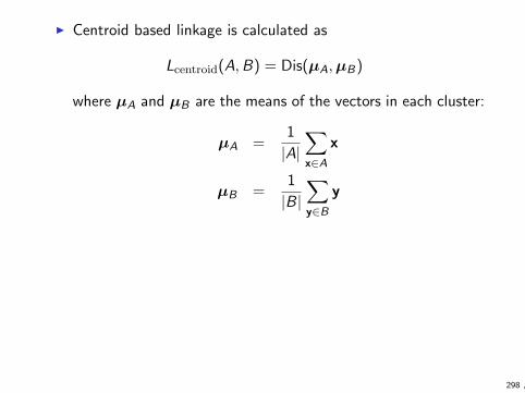
I Centroid based linkage is calculated as
Lcentroid(A,B) = Dis(µA,µB)
where µA and µB are the means of the vectors in each cluster:
µA =1
|A|∑
x∈Ax
µB =1
|B|∑
y∈By
298 ,

Example 1:8.3 Agglomerative Hierarchical Clustering 519
0.6
0.5
0.4
0.3
0.2
0.1
0
52
3
4
6
1
0 0.1 0.2 0.3 0.4 0.5 0.6
Figure 8.15. Set of 6 two-dimensional points.
Point x Coordinate y Coordinatep1 0.40 0.53p2 0.22 0.38p3 0.35 0.32p4 0.26 0.19p5 0.08 0.41p6 0.45 0.30
Table 8.3. xy coordinates of 6 points.
p1 p2 p3 p4 p5 p6p1 0.00 0.24 0.22 0.37 0.34 0.23p2 0.24 0.00 0.15 0.20 0.14 0.25p3 0.22 0.15 0.00 0.15 0.28 0.11p4 0.37 0.20 0.15 0.00 0.29 0.22p5 0.34 0.14 0.28 0.29 0.00 0.39p6 0.23 0.25 0.11 0.22 0.39 0.00
Table 8.4. Euclidean distance matrix for 6 points.
Single Link or MIN
For the single link or MIN version of hierarchical clustering, the proximityof two clusters is defined as the minimum of the distance (maximum of thesimilarity) between any two points in the two different clusters. Using graphterminology, if you start with all points as singleton clusters and add linksbetween points one at a time, shortest links first, then these single links com-bine the points into clusters. The single link technique is good at handlingnon-elliptical shapes, but is sensitive to noise and outliers.
Example 8.4 (Single Link). Figure 8.16 shows the result of applying thesingle link technique to our example data set of six points. Figure 8.16(a)shows the nested clusters as a sequence of nested ellipses, where the numbersassociated with the ellipses indicate the order of the clustering. Figure 8.16(b)shows the same information, but as a dendrogram. The height at which twoclusters are merged in the dendrogram reflects the distance of the two clusters.For instance, from Table 8.4, we see that the distance between points 3 and 6
8.3 Agglomerative Hierarchical Clustering 519
0.6
0.5
0.4
0.3
0.2
0.1
0
52
3
4
6
1
0 0.1 0.2 0.3 0.4 0.5 0.6
Figure 8.15. Set of 6 two-dimensional points.
Point x Coordinate y Coordinatep1 0.40 0.53p2 0.22 0.38p3 0.35 0.32p4 0.26 0.19p5 0.08 0.41p6 0.45 0.30
Table 8.3. xy coordinates of 6 points.
p1 p2 p3 p4 p5 p6p1 0.00 0.24 0.22 0.37 0.34 0.23p2 0.24 0.00 0.15 0.20 0.14 0.25p3 0.22 0.15 0.00 0.15 0.28 0.11p4 0.37 0.20 0.15 0.00 0.29 0.22p5 0.34 0.14 0.28 0.29 0.00 0.39p6 0.23 0.25 0.11 0.22 0.39 0.00
Table 8.4. Euclidean distance matrix for 6 points.
Single Link or MIN
For the single link or MIN version of hierarchical clustering, the proximityof two clusters is defined as the minimum of the distance (maximum of thesimilarity) between any two points in the two different clusters. Using graphterminology, if you start with all points as singleton clusters and add linksbetween points one at a time, shortest links first, then these single links com-bine the points into clusters. The single link technique is good at handlingnon-elliptical shapes, but is sensitive to noise and outliers.
Example 8.4 (Single Link). Figure 8.16 shows the result of applying thesingle link technique to our example data set of six points. Figure 8.16(a)shows the nested clusters as a sequence of nested ellipses, where the numbersassociated with the ellipses indicate the order of the clustering. Figure 8.16(b)shows the same information, but as a dendrogram. The height at which twoclusters are merged in the dendrogram reflects the distance of the two clusters.For instance, from Table 8.4, we see that the distance between points 3 and 6
I Single-link:520 Chapter 8 Cluster Analysis: Basic Concepts and Algorithms
6
4
52
1
3
32
4
5
1
(a) Single link clustering.
0.2
0.15
0.1
0.05
03 6 2 5 4 1
(b) Single link dendrogram.
Figure 8.16. Single link clustering of the six points shown in Figure 8.15.
is 0.11, and that is the height at which they are joined into one cluster in thedendrogram. As another example, the distance between clusters {3, 6} and{2, 5} is given by
dist({3, 6}, {2, 5}) = min(dist(3, 2), dist(6, 2), dist(3, 5), dist(6, 5))
= min(0.15, 0.25, 0.28, 0.39)
= 0.15.
Complete Link or MAX or CLIQUE
For the complete link or MAX version of hierarchical clustering, the proximityof two clusters is defined as the maximum of the distance (minimum of thesimilarity) between any two points in the two different clusters. Using graphterminology, if you start with all points as singleton clusters and add linksbetween points one at a time, shortest links first, then a group of points isnot a cluster until all the points in it are completely linked, i.e., form a clique.Complete link is less susceptible to noise and outliers, but it can break largeclusters and it favors globular shapes.
Example 8.5 (Complete Link). Figure 8.17 shows the results of applyingMAX to the sample data set of six points. As with single link, points 3 and 6
(The heights in the dendrogram correspond to linkage functionsLsingle(A,B) when clusters A and B are combined.)
299 ,
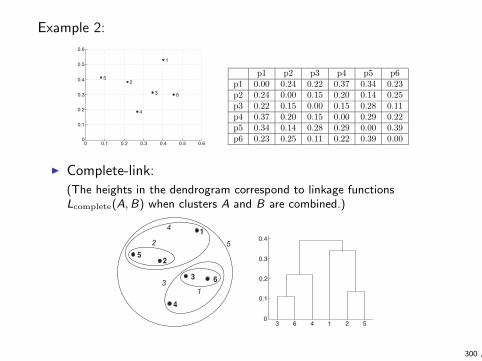
Example 2:8.3 Agglomerative Hierarchical Clustering 519
0.6
0.5
0.4
0.3
0.2
0.1
0
52
3
4
6
1
0 0.1 0.2 0.3 0.4 0.5 0.6
Figure 8.15. Set of 6 two-dimensional points.
Point x Coordinate y Coordinatep1 0.40 0.53p2 0.22 0.38p3 0.35 0.32p4 0.26 0.19p5 0.08 0.41p6 0.45 0.30
Table 8.3. xy coordinates of 6 points.
p1 p2 p3 p4 p5 p6p1 0.00 0.24 0.22 0.37 0.34 0.23p2 0.24 0.00 0.15 0.20 0.14 0.25p3 0.22 0.15 0.00 0.15 0.28 0.11p4 0.37 0.20 0.15 0.00 0.29 0.22p5 0.34 0.14 0.28 0.29 0.00 0.39p6 0.23 0.25 0.11 0.22 0.39 0.00
Table 8.4. Euclidean distance matrix for 6 points.
Single Link or MIN
For the single link or MIN version of hierarchical clustering, the proximityof two clusters is defined as the minimum of the distance (maximum of thesimilarity) between any two points in the two different clusters. Using graphterminology, if you start with all points as singleton clusters and add linksbetween points one at a time, shortest links first, then these single links com-bine the points into clusters. The single link technique is good at handlingnon-elliptical shapes, but is sensitive to noise and outliers.
Example 8.4 (Single Link). Figure 8.16 shows the result of applying thesingle link technique to our example data set of six points. Figure 8.16(a)shows the nested clusters as a sequence of nested ellipses, where the numbersassociated with the ellipses indicate the order of the clustering. Figure 8.16(b)shows the same information, but as a dendrogram. The height at which twoclusters are merged in the dendrogram reflects the distance of the two clusters.For instance, from Table 8.4, we see that the distance between points 3 and 6
8.3 Agglomerative Hierarchical Clustering 519
0.6
0.5
0.4
0.3
0.2
0.1
0
52
3
4
6
1
0 0.1 0.2 0.3 0.4 0.5 0.6
Figure 8.15. Set of 6 two-dimensional points.
Point x Coordinate y Coordinatep1 0.40 0.53p2 0.22 0.38p3 0.35 0.32p4 0.26 0.19p5 0.08 0.41p6 0.45 0.30
Table 8.3. xy coordinates of 6 points.
p1 p2 p3 p4 p5 p6p1 0.00 0.24 0.22 0.37 0.34 0.23p2 0.24 0.00 0.15 0.20 0.14 0.25p3 0.22 0.15 0.00 0.15 0.28 0.11p4 0.37 0.20 0.15 0.00 0.29 0.22p5 0.34 0.14 0.28 0.29 0.00 0.39p6 0.23 0.25 0.11 0.22 0.39 0.00
Table 8.4. Euclidean distance matrix for 6 points.
Single Link or MIN
For the single link or MIN version of hierarchical clustering, the proximityof two clusters is defined as the minimum of the distance (maximum of thesimilarity) between any two points in the two different clusters. Using graphterminology, if you start with all points as singleton clusters and add linksbetween points one at a time, shortest links first, then these single links com-bine the points into clusters. The single link technique is good at handlingnon-elliptical shapes, but is sensitive to noise and outliers.
Example 8.4 (Single Link). Figure 8.16 shows the result of applying thesingle link technique to our example data set of six points. Figure 8.16(a)shows the nested clusters as a sequence of nested ellipses, where the numbersassociated with the ellipses indicate the order of the clustering. Figure 8.16(b)shows the same information, but as a dendrogram. The height at which twoclusters are merged in the dendrogram reflects the distance of the two clusters.For instance, from Table 8.4, we see that the distance between points 3 and 6
I Complete-link:
(The heights in the dendrogram correspond to linkage functionsLcomplete(A,B) when clusters A and B are combined.)
8.3 Agglomerative Hierarchical Clustering 521
6
4
52
1
33
2
4
5
1
(a) Complete link clustering.
0.4
0.3
0.2
0.1
03 6 4 1 2 5
(b) Complete link dendrogram.
Figure 8.17. Complete link clustering of the six points shown in Figure 8.15.
are merged first. However, {3, 6} is merged with {4}, instead of {2, 5} or {1}because
dist({3, 6}, {4}) = max(dist(3, 4), dist(6, 4))
= max(0.15, 0.22)
= 0.22.
dist({3, 6}, {2, 5}) = max(dist(3, 2), dist(6, 2), dist(3, 5), dist(6, 5))
= max(0.15, 0.25, 0.28, 0.39)
= 0.39.
dist({3, 6}, {1}) = max(dist(3, 1), dist(6, 1))
= max(0.22, 0.23)
= 0.23.
Group Average
For the group average version of hierarchical clustering, the proximity of twoclusters is defined as the average pairwise proximity among all pairs of pointsin the different clusters. This is an intermediate approach between the singleand complete link approaches. Thus, for group average, the cluster proxim-
300 ,
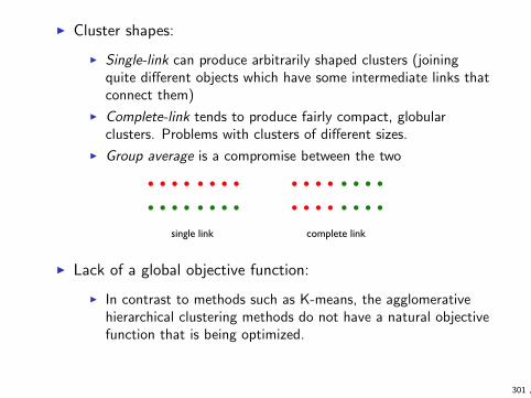
I Cluster shapes:
I Single-link can produce arbitrarily shaped clusters (joiningquite different objects which have some intermediate links thatconnect them)
I Complete-link tends to produce fairly compact, globularclusters. Problems with clusters of different sizes.
I Group average is a compromise between the two
single link complete link
I Lack of a global objective function:
I In contrast to methods such as K-means, the agglomerativehierarchical clustering methods do not have a natural objectivefunction that is being optimized.
301 ,

I Monotonicity:
If the dissimilarity between a pair clusters merged at any point in thealgorithm is always at least as large as the dissimilarity of the pair ofclusters merged in the previous step, the clustering is monotonic.
I Single-link, complete-link, and group average: Yes!
I Centroid-based hierarchical clustering: No! Example:
d1 = (1 + ε, 1), d2 = (5, 1), d3 = (3, 1 + 2√
3).The first combination (of d1 and d2) occurs ata distance of 4− ε. The point o = (3 + ε/2, 1).The next combination occurs at distance of√
(2√
3)2 + (ε/2)2 ≈ 2√
3 ≈ 3.4641 < 4− ε
�= ( + �, ) = ( , )
− �= ( , +
√)
= ( + �/ , )
√+ �/ ≈ . + �/
�
�302 ,
I Computational complexity
I The main storage requirement is the matrix of pairwisedistances, containing a total of N(N − 1)/2 entries for Ndatapoints. So the space complexity is: O(N2).
I Computing the distance matrix takes O(N2). Next, there areO(N) iterations, where in each one we need to find theminimum of the pairwise dissimilarities between the clusters.Trivially implemented this would lead to an O(N3) algorithm,but techniques exist to avoid exhaustive search at each step,yielding complexities in the range O(N2) to O(N2 log N).
(Compare this to K-means, which only requires O(NK ) for Kclusters.)
Hence, hierarchical clustering is directly applicable only torelatively small datasets.
303 ,

Clustering: summary
I K-means and hierarchical clustering are among the main toolsin data analysis. Everyone in the area must understand
I what the algorithms do
I how to interpret the results
I computational and other limitations of the algorithms
I Often goal is understanding the data, with no clearly definedprediction or other task
I difficult to define good performace metrics
I difficult to give good procedures for “model selection” (e.g.choosing number of clusters)
304 ,

Clustering in textbook
I We followed the textbook rather closely
I Introduction to clustering: pages 95–99
I Distance-based clustering: Section 8.4
I Hierarchical clustering: Section 8.5
I Further important topics in the textbook, not covered inlectures, include
I kernel-based clustering (Section 8.6)
I soft clustering and the EM algorithm (Section 9.4)
305 ,

Matrix Decompositions
306 ,
Singular Value Decomposition
I Consider an m × n matrix X where m > n
I It can be shown that we can decompose X as
X = UΣV T
whereI U is m by n matrix whose columns are orthogonal unit vectors;
its colums are called left singular vectors of X
I V is n by n matrix whose columns are orthogonal unit vectors;its colums are called right singular vectors of X
I Σ is diagonal n by n matrix; the values on its diagonal arecalled singular values of X
I This is known as singular value decomposition (SVD) of XI Sometimes this is called reduced SVD, in contrast to “full”
SVD where U is m by m and Σ is m by n
307 ,

Singular Value Decomposition (2)
I Singular values of a matrix are uniquely defined, and if thematrix is square and the singular values distinct, so are thesingular vectors (up to changing sign)
I SVD can be computed in time O(n2m)
I Notation:I columns of U are u1, . . . ,unI columns of V are v1, . . . , vnI singular values are σ1 ≥ · · · ≥ σn
308 ,
Singular Value Decomposition (3)
I To understand how SVD works, consider calculatingXw = UΣV Tw in stages:
p = V Tw
q = Σp = ΣV Tw
r = Uq = UΣV Tw
I Since v1, . . . , vn are n orthogonal vectors in Rn, they form abasis, and we can write
w = a1v1 + · · ·+ anvn
where ai = vTi w
I Then pi = (V Tw) = vTi w = ai
309 ,
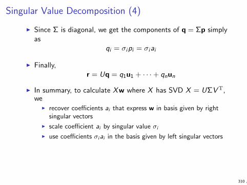
Singular Value Decomposition (4)
I Since Σ is diagonal, we get the components of q = Σp simplyas
qi = σipi = σiai
I Finally,r = Uq = q1u1 + · · ·+ qnun
I In summary, to calculate Xw where X has SVD X = UΣV T,we
I recover coefficients ai that express w in basis given by rightsingular vectors
I scale coefficient ai by singular value σiI use coefficients σiai in the basis given by left singular vectors
310 ,

Low rank approximation
I Given the left singular vectors ui , right singular vectors vi andsingular values σi , we can also write
X =n∑
i=1
σiuivTi
I We can then approximate X by keeping only the termscorresponding to r largest singular values:
X ≈ X =k∑
i=1
σiuivTi
311 ,
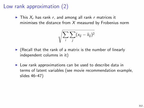
Low rank approximation (2)
I This Xr has rank r , and among all rank r matrices itminimises the distance from X measured by Frobenius norm
√∑
i
∑
j
(xij − xij)2
I (Recall that the rank of a matrix is the number of linearlyindependent columns in it)
I Low rank approximations can be used to describe data interms of latent variables (see movie recommendation example,slides 46–47)
312 ,

Principal Componenent Analysis
I Principal Component Analysis is a common dimensionalityreduction technique
I The basic idea is to project the data onto a lower dimensionalsubspace so that as much variance as possible is retained
I Assume from now on that data is zero-centeredI If the original instances are x′1, . . . , x
′n, we replace them by
xi = x′i − x′ where x′ = 1n
∑ni=1 x
′i
I Then∑
i xi = 0 and therefore xj = 0 for j = 1, . . . , d
313 ,

Principal Componenent Analysis (2)
I Substitute now X = UΣV T into the scatter matrix S = XTX :
S = XTX = V ΣTUTUΣV T = V Σ2V T
since columns of U are orthogonal and Σ is diagonal
I This is the Eigenvalue decomposition of S . Each column vi ofV is an Eigenvector of S with the corresponding Eigenvalueσ2i :
Svi = σ2i vi
I In general, any symmetrical matrix has an Eigenvaluedecomposition
314 ,

Principal Componenent Analysis (3)
I Pick now a unit vector u ∈ Rd and project all instances xialong direction u
I The projection of xi is uTxi , and the variance of theprojections is
n∑
i=1
(uTxi )2 =
n∑
i=1
(Xu)2i = uTXTXu
(recall the data is zero-centered)
I It is fairly easy see that the unit vector u that maximises thisis the Eigenvector of XTX corresponding to the largestEigenvalue. We call this the first principal component of thedata
315 ,

Principal Componenent Analysis (4)
I In Principal Component Analysis (PCA) we first findv1, . . . , vk , the Eigenvectors corresponding to k largestEigenvalues of XTX
I Then xi is replaced by its projection x′i onto subspace spannedby v1, . . . , vk :
x′i = (vT1 xi , . . . , vTk xi )
I Among all possible linear projections of the data onto a kdimensional subspace, this method
I maximises the variance of x′iI minimises the “squared error”
∑i ‖xi − x′i‖
22
I Other dimensionality reduction techniques includeIndependent Component Analysis and Factor Analysis
316 ,
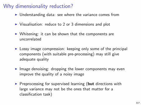
Why dimensionality reduction?
I Understanding data: see where the variance comes from
I Visualisation: reduce to 2 or 3 dimensions and plot
I Whitening: it can be shown that the components areuncorrelated
I Lossy image compression: keeping only some of the principalcomponents (with suitable pre-processing) may still giveadequate quality
I Image denoising: dropping the lower components may evenimprove the quality of a noisy image
I Preprocessing for supervised learning (but directions withlarge variance may not be the ones that matter for aclassification task)
317 ,

Where to go next?
I Advanced Course in Machine Learning
I Probabilistic Models (with optional project)
I Data Mining (with optional project)
I Project in Practical Machine Learning
I Several seminars on machine-learning related topics
I Courses at maths department
I Courses at Aalto University
I Online courses
The End
318 ,