584 multivariate approximation(u) … · ams (mos) subject classifications: 41-02, ... preventive...
TRANSCRIPT
AD-Ai72 584 MULTIVARIATE APPROXIMATION(U) ;ISCONSIN UNdV-MADISONMATHENATICS RESEARCH CENTER C DE BOOR AUG 86MRC-TSR-2950 DARG29-80-C-8e4i
UNCLASSIFIED F/G 12/1 NLME EEEEEEmmEmmmmmmmm7mmmmm
1L -

1111 1.0112.0m1.8
1I11.25 11tH1J.4 .
MICROCOPY RESOLUTION TEST CHARTNATIONAL BUREAU OF STANDARDS 1963-A
MRC Technical Summary Report #2950
MULTIVARIATE APPROXIMATION
aCarl de Boor
i in
Mathematics Research CenterUniversity of Wisconsin-Madison
610 Walnut StreetMadison, Wisconsin 53705 DTIC
August 1986 OCT8 1 86
B. - (Received June 19, 1986)
Approved for public release
___ Distribution unlimited
Sponsored by
U. S. Army Research OfficeP. O. Box 12211Research Triangle ParkNorth Carolina 27709
86 10 7 16
UNIVERSITY OF WISCONSIN-MADISONMATHEMATICS RESEARCH CENTER
MULTIVARIATE APPROXIMATION
Carl de Boor
Technical Summary Report #2950August 1986
ABSTRACT
The lecture addresses topics in multivariate approximation which have caught theauthor's interest in the last ten years. These include: the approximation by functionswith fewer variables, correct points for polynomial interpolation, the B(ernstein,-zier,-arycentric)-form for polynomials and its use in understanding smooth pp functions, approx-imation order from spaces of pp functions. multivariate B-splines, and surface generationby subdivision.
AMS (MOS) Subject Classifications: 41-02, 41A05, 41A10, 41A15, 41A63, 41A65
Key Words: multivariate, interpolation, B-form, subdivision, splines, B-splines
Work Unit Number 3 - Numerical Analysis and Scientific Computing
i
tV- Sponsored by the United States Army under Contract No. DAAG29-80-C--041.
%
/' , ., :.''L, .'(, ,L , * " r, ,-.r.-..r .. " .' ,,, . ,._ '. ' " "" " " € ¢' €"¢ ".-Z "d --°
': " "-' -'¢ -'"": ' " ". . """ I

SIGNIFICANCE AND EXPLANATION
This lecture was given at the IMA SIAM conference on "State of the Art in NumericalAnalysis" held April 14-18. 1986, in Birmingham. England. The lecture reviews develop-ments in Multivariate Approximation in the last ten years. The selection of topics is quitesubjective; it reflects entirely the author's research experience during that time.
NTISDT!
Dist
/t
( -~P, ',"B
The responsibility for the wording and views expressed in this descriptive summary lieswith MRC, and not with the author of this report.
N,% , oP -
MULTIVARIATE APPROXIMATION
Carl de Boor
1. The set-up
The talk concerns the approximation of
f : G C Rd ---+ IR,
i.e., of some real-valued function f defined on some domain G in d-dimensional space.
While my first publication dealt with such multivariate (actually, bivariate) approxi-
mation, I have concerned myself seriously with multivariate approximation only in the last
ten years. This talk reflects some of the experiences I have had during that time.
The approximating functions are typically polynomials or piecewise polynomials, and
just how one describes them will have an effect on one's work with them. Papers on
multivariate approximation often sink under the burden of cumbersome notation. As a
preventive measure against such a sad fate, I shall follow the "default" convention whereby
symbols are left out if they can reasonably be guessed from the context. For example, if
zx = (z(1),. .. ,(d)) has just been declared to be a point in IR , I will feel free to write
Zx (i) instead of x (i).
For polynomials, multi-index notation is standard. With z = (x(1),...,z(d)) the
generic point in IR d, one uses the abbreviation
X f= z () ), E IR aEZ.i
The function x - x* is a monomial of degree a, or, of (total) degree
:=l Z(i)
if only the exponent sum matters. More generally. a polynomial of degree < a is, by
definition, any function of the form
X -3
Sponsored by the United States Army under Contract No. DAAG29-80-C-0041.
"> -'2 2 . " . . . , , ,, " .
2 Carl de Boor
with real coefficients c(3). The collection of all such polynomials is denoted by
70- = 7(IRd),
the collection of all polynomials of total degree at most k by
7rk 7k(IRd),
and the collection of all polynomials, of whatever degree, by
7r= 7(d).
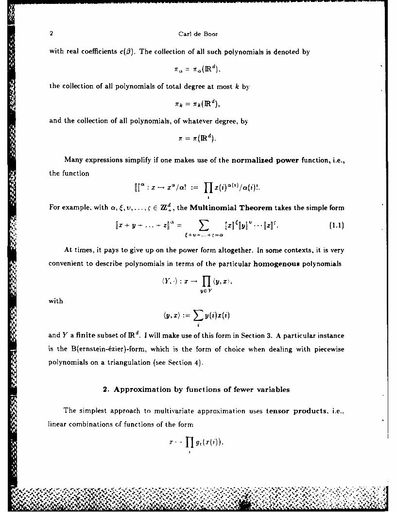
Many expressions simplify if one makes use of the normalized power function, i.e.,
the function
:X-X,/! := 1X(iy2(1)/a()!For example. with a, C, v..., c E Md, the Multinomial Theorem takes the simple form
±x + ...- ,- 4 N j' M' .. j. (1.1)
At times, it pays to give up on the power form altogether. In some contexts, it is very
convenient to describe polynomials in terms of the particular homogenous polynomials
•Y X : H - (Y, XI),
YEY
with
(YX) ZY(0 X (2)
and Y a finite subset of IRd. I will make use of this form in Section 3. A particular instance
is the B(ernstein-6zier)-form, which is the form of choice when dealing with piecewise
polynomials on a triangulation (see Section 4).
2. Approximation by functions of fewer variables
The simplest approach to multivariate approximation uses tensor products, i.e.,
linear combinations of functions of the form
g 9 ( .
%1
~ ,,a

Multivariate Approximation 3
each g1 being a univariate function. This neatly avoids dealing with the realities of multi-
variate functions, but its effectiveness depends on having the information about I corre-
spondingly available in (cartesian) product form, e.g., as function values on a rectangular
grid parallel to the coordinate axes. The recent book by Light and Cheney (1986) provides
*up-to-date material on this practically very important choice of approximating function
and certain ready extensions.
The book also deals with the situation when the information about f is not in product
form. In that case, tensor product approximants still are attractive since they are composed
of univariate functions. The general question of how to approximate a multivariate function
by functions of fewer variables has received much attention. A reference with a Numerical
Analysis slant is Golomb (1959).
The most remarkable result along this line is
Kolmogorov's Theorem (Kolmogorov, 1957)
3A Eo, lj d , 30 C Lip[0, i n strictly monotone, #0 = 2d + 1, such that
Vf E C[0,ld B3g ECO,dI
f(z) W 7 g( ZA(i)p (z(i)))" (2.1)
(Here and below,
#A := the number of elements in A.)
The theorem claims the existence of a set %P of 2d+ 1 'universal' maps 'k :10, 1 ]d -- [0,d]
so that, for each continuous function f on the unit cube [0, 1 Id, a continuous function g on
the interval [0, dj can be found for which
f =- E go P..E
Moreover, each function aV E %P is of the form
dOX() := A(i)P(-(i)),
T::
S ,-..,. .: .. ,.:2: .,- . . ,. - _ , . . . . . . . . . . . . . . . . , ,. . . . , . . . . .
,?., ,. .. , ., .,-.-., : . .. , .-:- .. ... -... ... ... .. ,. ,... .,-,.-.,-..,..• .- , ....... .. . ... . .. .:..,., ..-........ ... ,..'..-- .
4 Carl de Boor
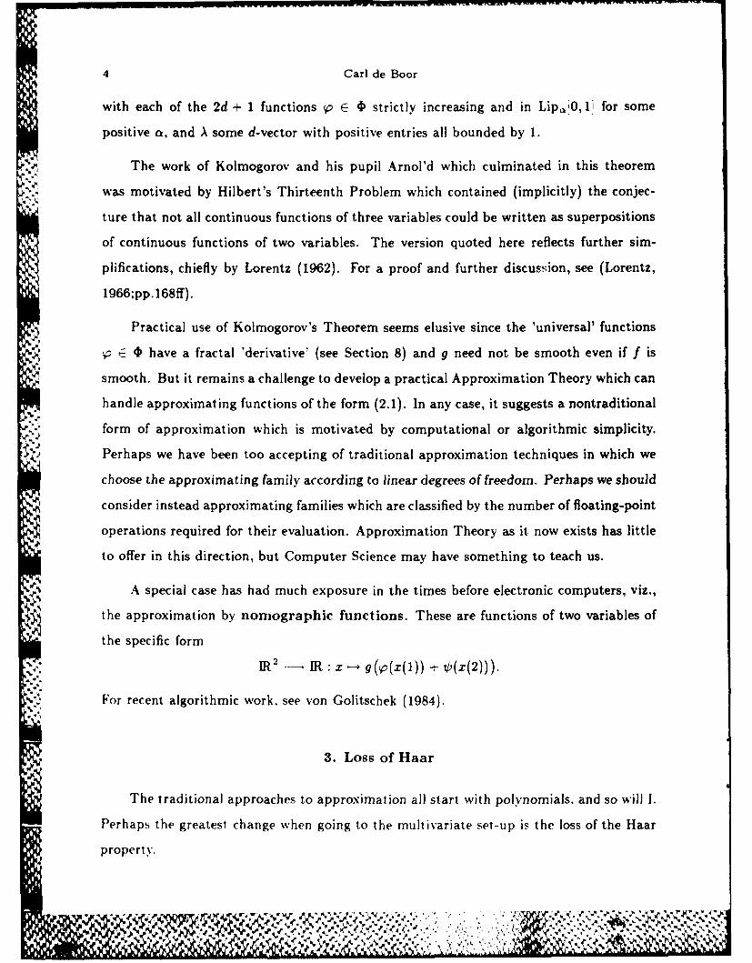
with each of the 2d + 1 functions p e 0 strictly increasing and in Lip,,0, 1i for some
positive Q, and A some d-vector with positive entries all bounded by 1.
The work of Kolmogorov and his pupil Arnol'd which culminated in this theorem
was motivated by Hilbert's Thirteenth Problem which contained (implicitly) the conjec-
ture that not all continuous functions of three variables could be written as superpositions
of continuous functions of two variables. The version quoted here reflects further sim-
plifications, chiefly by Lorentz (1962). For a proof and further discussion, see (Lorentz,
1966;pp. 168ff).
Practical use of Kolmogorov's Theorem seems elusive since the 'universal' functions
E 0 have a fractal 'derivative' (see Section 8) and g need not be smooth even if f is
smooth. But it remains a challenge to develop a practical Approximation Theory which can
handle approximating functions of the form (2.1). In any case, it suggests a nontraditional
form of approximation which is motivated by computational or algorithmic simplicity.
Perhaps we have been too accepting of traditional approximation techniques in which we
choose the approximating family according to linear degrees of freedom. Perhaps we should
consider instead approximating families which are classified by the number of floating-point
operations required for their evaluation. Approximation Theory as it now exists has little
to offer in this direction, but Computer Science may have something to teach us.
A special case has had much exposure in the times before electronic computers, viz.,
the approximation by nomographic functions. These are functions of two variables of
the specific form
. IR 2 -- IR :x - g(p (x(m)) -t-, V(x(2))).
,, For recent algorithmic work. see von Golitschek (1984).
3. Loss of Haar
The traditional approaches to approximation all start with polynomials, and so will 1.
Perhaps the greatest change when going to the multivariate set-up is the loss of the Haar
property.
'A::

Multivariate Approximation 5
To recall, interpolation from a linear space S of functions on some G C IRd at a point
set T c G can be viewed as the task of inverting the restriction map
S - IR T : p _-- P;T.
We are to (re)construct some element p E S from its prescribed values pT at the points in
T. In these terms, S has the Haar property if every T Z G with #T = dimS is correct
for S, i.e., is such that
S - IRT : P - PIT is 1-1 and onto.
In other words, we can interpolate, and uniquely so, from S to any function values given
on T.
If d = 1. then Irk has the Haar property (for any G with more than k points), but
Mairhuber's switching yard argument (cf., e.g., the cover of Lorentz (1966)) shows that
Z.: this property cannot hold for any S of dimension > 1 on a multidimensional set G.
For the case of polynomials, it is possible to identify various point sets T C IRd which
are correct for 7rk. A particularly nice example is provided by Chung and Yao (1977) who
prove the following: Suppose that V is a finite subset of Rd\0, and that V u0 is in general
position, which means that 7r, has the Haar property on V u 0. This implies that for
every W c V with #W = d, xw E IRd is defined uniquely by the equations
1 - (w, xw) = O. w E W,
since these state that the linear polynomial 1 - (.. .w;, is to vanish on W and take the
value 1 at 0. Further. since 1 + (., Xw) already vanishes on the d points in W, it cannot
vanish anywhere on V\W, by the Haar property. It follows that the functions
(w~x- H I V.X'c- 1, VVv,
are well-defined, are made up of F V - d linear factors. and satisfy (w,(xw,) = 6ww, (since.
for W' W. at least one v J V W is in IW". making the corresponding linear factor zero at
• --. " ' . " - I -.-. '" - , .- I, PS. .1
6 Carl de Boor
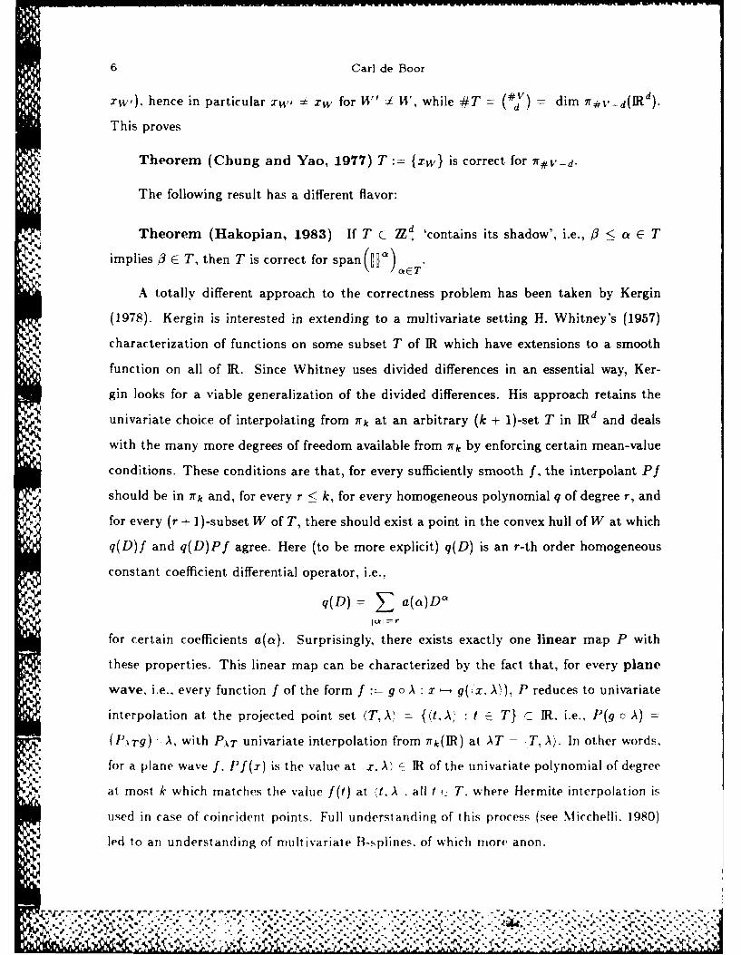
xw,). hence in particular x, i xw for W' : W, while #T = (#dV) = dim 7#V-d(,Rd).
This proves
Theorem (Chung and Yao, 1977) T := {xwl is correct for ir#v-d.
The following result has a different flavor:
Theorem (Hakopian, 1983) If T c d 'contains its shadow', i.e., /3 < a E T
implies 4 E T, then T is correct for span(nk) T.
A totally different approach to the correctness problem has been taken by Kergin
(1978). Kergin is interested in extending to a multivariate setting H. Whitney's (1957)
characterization of functions on some subset T of IR which have extensions to a smooth
function on all of IR. Since Whitney uses divided differences in an essential way, Ker-
gin looks for a viable generalization of the divided differences. His approach retains the
univariate choice of interpolating from 7rk at an arbitrary (k + 1)-set T in IRd and deals
with the many more degrees of freedom available from irk by enforcing certain mean-value
conditions. These conditions are that, for every sufficiently smooth f, the interpolant Pf
should be in 7rk and, for every r < k, for every homogeneous polynomial q of degree r, and
for every (r + 1)-subset W of T, there should exist a point in the convex hull of W at which
q(D)f and q(D)Pf agree. Here (to be more explicit) q(D) is an r-th order homogeneous
constant coefficient differential operator, i.e..
~q(D) a a) D
for certain coefficients a(a). Surprisingly, there exists exactly one linear map P with
these properties. This linear map can be characterized by the fact that, for every plane
wave. i.e.. every function f of the form f := g o A x - g(kx. A')j P reduces to univariate
interpolation at the projected point set (T, Al {(tAL : t : T} C IR. i.e., P(g c A) =
(Pt g) - A, with PAT univariate interpolation from 7rk(IR) at AT = :T, A). In other words.
for a plane wave f. Pf(i) is the value at x. A, - IR of the univariate polynomial of degree
at most k which matches the value f(t) at 't. A all f f- T. where Hermite interpolation is
used in case of coincident points. Full understanding of this process (see Micchelli. 1980)
led to an understanding of multivariate B-splines. of which more anon.
A. % s. % JAA

Multivariate Approximation 7
It seems more promising to give up on polynomials altogether and to choose the
interpolating function space S to depend on the point set T at which data are given. The
simplest general model has the form
E P(. - t)c(t),tET
with P IR d -- IR a function to be chosen 'suitably'. Duchon's thin plate splines (see,
e.g., Meinguet, 1979) use
PX =IXlIrn-d 1 lrjxj' n even;1, 1, n odd,
motivated by a variational argument, while Hardy's multiquadrics correspond to the
choice., := 1±f + 1
A good source of up-to-date information about such interpolation methods and, in par-
ticular, about the question of their correctness, is the recent survey article of Micchelli
(1986).
4. The B-form
I now come to a discussion of piecewise polynomial functions, or pp functions for
short. I have learned from the people in Computer-Aided Geometric Design that, in dealing
with smooth pp functions on some triangulation, it is usually advantageous to write the
polynomial pieces in barycentric-Bernstein-Bdzier form, or B-form for short. This
form relates polynomials to a given simplex. It is hard to appreciate the power and beauty
of this form because, even with carefully chosen notation, it looks forbidding at first sight.
Still, I want to point out its structure at least.
One starts with a (d-t- 1)-subset V of IRd in general position and considers the barycen-
tric coordinates with respect to it. i.e.. the Lagrange polynomials for linear interpolation
at V. The typical Lagrange polynomial c takes the value 1 at the vertex v and vanishes
~ %
Carl de Boor
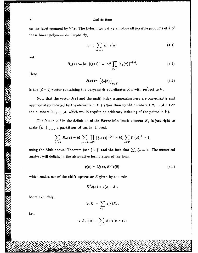
on the facet spanned by V\v. The B-form for p E 7rk employs all possible products of k of
these linear polynomials. Explicitly,
P=: > Bo c(a) (4.1)
with
B.(x) :=!f (x) = a'! J I(xWl' ) (4.2)vEV
Here
is the (d -t 1)-vector containing the barycentric coordinates of x with res'pect to V.
Note that the vector C(x) and the multi-index a appearing here are conveniently and
appropriately indexed by the elements of V (rather than by the numbers 1, 2,..., d + 1 or
the numbers 0, 1,...,d. which would require an arbitrary indexing of the points in V).
The factor IaI! in the definition of the Bernstein basis element B, is just right to
make (B 0 )1= k a partition of unity. Indeed.
E Ba(x) = k! : 1 Cv(x)"a(v)= k! E Cv(x)k = 1,IoI=k JI=k vEV vEV
using the Multinomial Theorem (see (1.1)) and the fact that , = 1. The numerical
analyst will delight in the alternative formulation of the form,
p(x) = (C(x), E)'c(O) (4.4)
which makes use of the shift operator E given by the rule
Efbc(a) - (a -- 3).
More explicitly,
z'c 2-09E,.
z. E;c (a) - OW L~zv C ')
Multivariate Approximation 9
with e, the v-unitvector, i.e, e,(w) = i w r V. This form provides a most convenient
starting point for the derivation of efficient algorithms for the evaluation and differentiation
of the B-form. For details, see, e.g., Farin (1985) and de Boor (1986).
5. Smooth pp functions
The B-form is well suited to pp work since its typical term B, vanishes a(v)-fold on
the facet spanned by V\v. This means that the form readily provides information about
the behavior of p at all the bounding faces of the simplex with vertex set V. This is being
increasingly exploited in studying the algebraic structure of the space
e, 7rk,A
of pp functions of degree < k on a given triangulation A whose pieces join together
smoothly to provide a function all of whose derivatives of order < p are continuous.
The problems being studied include: the dimension of such a space, a good basis for
such a space, and the approximation power of such a space. For recent results, see Chui
and his co-workers, and Schumaker. These results only deal with d = 2, and, even for this
case. we know relatively little. For example, despite considerable efforts, we still do not
know the dimension of the space of continuously differentiable piecewise cubic functions
on an arbitrary triangulation in the plane. While we do know that this dimension depends
on the quantitative details of the triangulation, we do not know exactly how.
As we understand these problems better and see some of their particular difficulties.
we wonder whether 7rP, is really the right space to study. It now seems that it might
be more appropriate to seek out appropriate subspaces, e.g., the subspace spanned by
certain compactly supported smooth piecewise polynomials as was done already in Finite
Elements. A particularly simple model is provided by approximation from a scale of pp
functions.
% .'
,ea
10 Carl de Boor
6. Approximation from a scale
Associate with a given function space S the scale (Sh), with
Sh := UhS, (af)(x) := f(x/h),
and define the approximation order of S to be
max {r : V smooth f dist(f, Sh) : O(hT )}.
This order may well be 0, as it is for S = 7rk. But if S contains functions whose support
has diameter 6, then Sh contains functions with supports of diameter h6. and, for such
S, one might hope to obtain closer approximations from Sh as h - 0. Work with specificexamples has suggested the following conjectures in case S C 7rk,A:
Conjectures: (i) The approximation order of S equals the approximation order of
Sloc := span {p C S : supp p compact}.
(ii) S has approximation order > 1 iff S contains a local partition of unity.
(iii) The approximation order is always realized by a good quasi-interpolant.
Here, a map Q into S is a good quasi-interpolant of order r in case it is a linear
map which is stable in the sense that, for any f and any x C- G,
I(Qf)(x)! < constsup{If(y) : y- xl' -- R}
with const and R < oc independent of f or x. and which reproduces polynomials of
degree - r. For example, if -t is a local and nonnegative partition of unity in S, i.e.,
sups. Vdiamsuppp< oc,, >0forallnE b,andZ' , 1, then
f ~- : f (7r)
is a good quasi-interpolant of order 1 (provided. e.g.. that T,, suppp for all t ,i ).
A,,. ! IUR
Multivariate Approximation 11
This abstract model can be completely analysed in the very special case when S is
spanned by the integer translates of one function p, i.e.,
S : SW:= span(P(' -J)), = { E P(' - j)c(j) :c(j) E IR}.
For this case, the three conjectures are verified; in particular, Strang and Fix (1973) prove
that S has approximation order r iff ?r<, C S.
Already for the slightly more general case when S is the span of integer translates of
several compactly supported functions, the situation becomes more complicated. A char-
acterization of the approximation order is not yet known for this case, but the somewhat
stronger (and practically more interesting) concept of local approximation order can be
characterized very simply (de Boor and Jia, 1985): S has local approximation order
r iff there exists tk E SIoc such that So has approximation order r.
For the general case, even simple questions such as whether a pp space with positive
approximation order must contain a compactly supported element have so far remained
unanswered.
7. Multivariate B-splines
The abstract theory of approximation from a scale has found new interest recently
because of the advent of multivariate B-splines. These were introduced in 1976 in hopes
that they would perform the same service in the study of multivariate smooth pp functions
that the B-splines of Schoenberg and Curry provided so nicely for the theory of (univariate)
splines.
In retrospect, well, in any case, the idea is simple enough. It involves a body B , IR'
and the orthogonal projector P : IR" -. IRd : X -. ((1).... ,x(d)). The map P is used to
extend a function p on IRd to the function
or P : U - O(Pu)
-- v-

12 Carl de Boor
on all of IR'. The B-spline MB is defined as the distribution on IRd which represents
integration over B of the extended function. In formulae:
MB : - fB P o P for all p E Co. (7.1)
Here, Cc = Co(IRd) is the collection of all continuous functions on IRd with compactsupport. If PB (the projection of the body) is d-dimensional, this can also be written
SMB dyO(y) fB 1 (7.2)P B Bnp- 3 1
showing that MB(y) = voldB n P-ly. This latter formula was the original definition,
motivated by a geometric characterization of the (univariate) B-spline due to Curry andSchoenberg (1966) and illustrated, for n = 3, d = 1, in Figure 7.1.
....
I'I
II
Figure 7.1 The quadratic B-spline as the "shadow" of a 3-simplex.
The value of the B-spline at a point y equals the (n - d)-dimensional volume of the
intersection of the simplex with the hyperplane P-my.
It is immediate that MB has compact support. Further, if B is polyhedral withfacets {B,}. and if z E IR"1 , then an application of Stokes' Formula shows that the direc-
tional derivative of MB along Pz is
DpMB - Zr.nz mp,. (8.1)
iUPI
Multivariate Approximation 13
with ni the outward unit normal to the facet B, and MB, the B-spline that is the "shadow"
of the "body" B,. Repeated applications of this differentiation formula show that all
derivatives of MB of order n - d + 1 must vanish identically away from the projections of
the (d - 1)-dimensional faces of B. Consequently,
MB E 7n-d,A1
with A the partition whose partition interfaces are the projections of (d -1)-dimensional
faces of B, and where p is defined by the condition that n-p-2 equal the largest dimension
of a face of B projected entirely into one of the partition interfaces. Thus, in the generic
case, we have p = n - d -1, which is as large as it can possibly be, given that the polynomial
degree of MB is n - d.
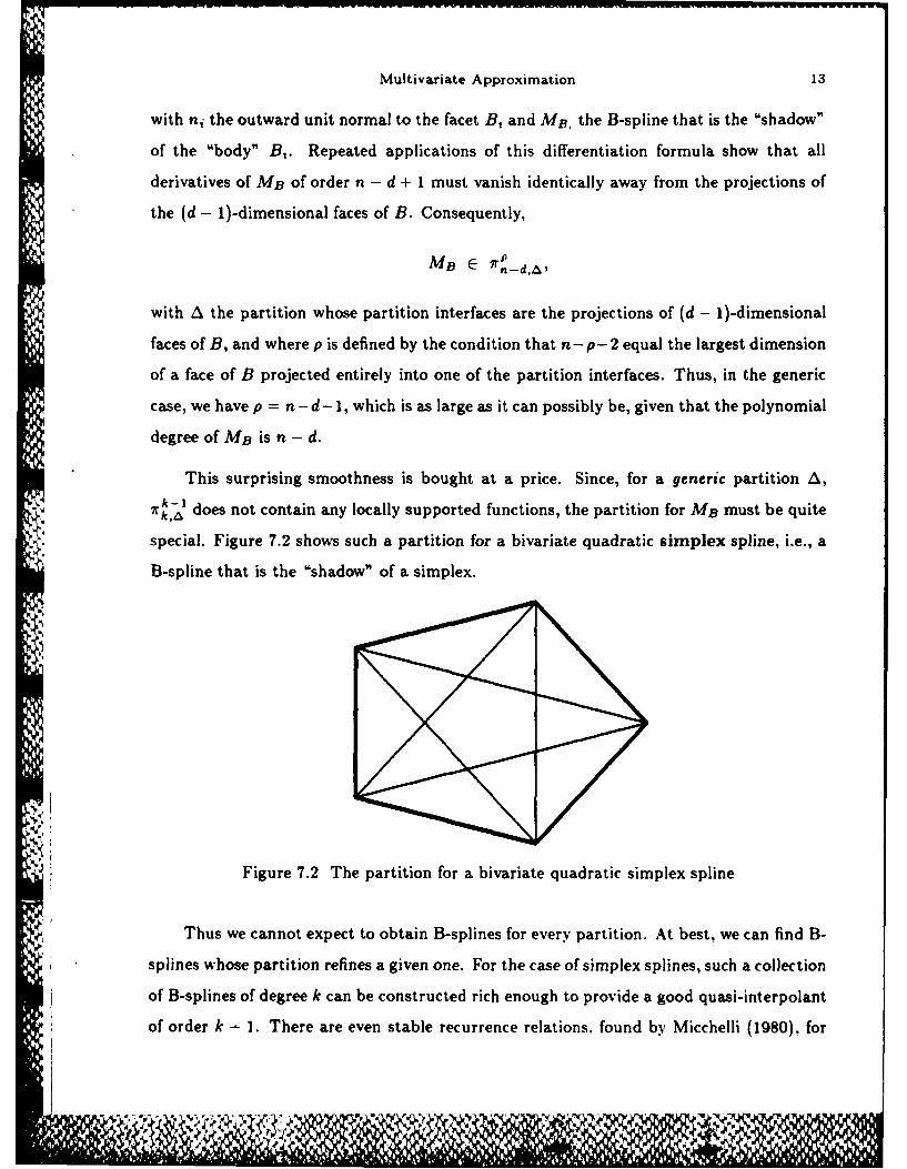
This surprising smoothness is bought at a price. Since, for a generic partition A,
7rk- does not contain any locally supported functions, the partition for MB must be quite
special. Figure 7.2 shows such a partition for a bivariate quadratic simplex spline, i.e., a
B-spline that is the "shadow" of a simplex.
Figure 7.2 The partition for a bivariate quadratic simplex spline
Thus we cannot expect to obtain B-splines for every partition. At best, we can find B-
splines whose partition refines a given one. For the case of simplex splines, such a collection
of B-splines of degree k can be constructed rich enough to provide a good quasi-interpolant
of order k - 1. There are even stable recurrence relations. found by Micchelli (1980), for
iI -

14 Carl de Boor
their evaluation. But it seems that their use is computationally quite expensive (see, e.g.,
Grandine, 1986). It is therefore not likely that simplex splines will be used as a basis for
a good subspace of a given smooth pp space of functions. Most likely, translates of a fixed
B-spline will find practical employment.
There is a bit more hope for the box splines, i.e., the multivariate B-splines associated
with the n-cube B = 10, 11n . For their definition in terms of (7.1), one would allow P to
be, more generally, a linear map. Then, with , := Pei the image of the i-th unit vector
under P, the box spline can be characterized more explicitly by
I M('l , ---'" ) = f o j,, Ciy(i))d ' , p Co.
By choosing the , from 2Zd appropriately, the resulting partition can be made to conform
to a regular grid; see Figure 7.3 for the supports of two very well known box splines, the
Courant element (d = 2,n = 3) and the Zwart-Powell element (d 2, n = 4). Further,
their evaluation can be accomplished by subdivision.
///
Figure 7.3 The supports of a linear and a quadratic bivariate box spline
De Boor (1982) gives an introduction to multivariate B-splines. Dahmen and Mic-
chelli (1984) provide a survey of the literature available by 1983 to which they heavily
contributed. H6llig (1986a) gives a more up-to-date introduction, and Hbllig (1986b) sum-
marizes what we know about box splines. In addition, I want to stress the beautiful. but
4 AA
Multivariate Approximation 15
more theoreticai, developments to which Dahmen and Micchelli were led by their intensive
study of box splines (see, e.g., Dahmen and Micchelli, 1985, 1986).
8. Subdivision
I hate to finish on a pessimistic note. I therefore bring up a totally different approach
to the generation or approximation of surfaces which comes from Computer-Aided Design.
I think that this technique has real promise for the generation of 'smooth' surfaces which
fit to given points in 3-space of more or less arbitrary combinatorial structure. It is at
$. present being used to evaluate linear combinations of box splines (see, e.g., H6llig, 1986a,
for the relevant references). But since this idea has not yet been thoroughly studied, I will
discuss it only in its original context of curve generation.
x
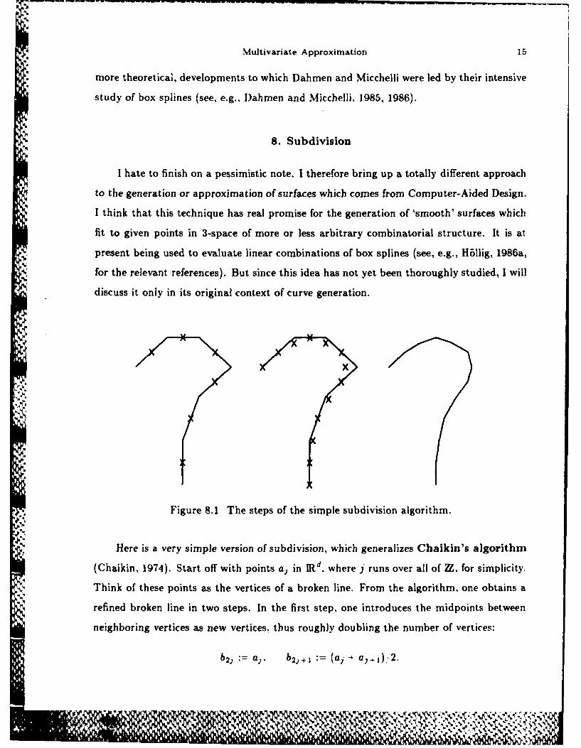
* Figure 8.1 The steps of the simple subdivision algorithm.
Here is a very simple version of subdivision, which generalizes Chaikin's algorithm
(Chaikin, 1974). Start off with points a, in IRd , where j runs over all of Z, for simplicity.
Think of these points as the vertices of a broken line. From the algorithm, one obtains a
refined broken line in two steps. In the first step, one introduces the midpoints between
neighboring vertices as new vertices, thus roughly doubling the number of vertices:
b4 := a.. b2j+ : (a, 1 ,'2.
Mb,

16 Carl de Boor
In the second step, one obtains each vertex of the refined broken line as an average of three
neighboring vertices:
c := bj- +ab 3 +-yb,+, with 03-.- a--y 1.
In fact, for a curve of higher 'smoothness', one would repeat this averaging step one or
more times, but I will stick with this simple model. Repetition quickly leads to a broken
line which, for plotting purposes, is indistinguishable from the limiting curve.
Of course, it is not at all clear a priori that there is a limiting curve, though that is
easily proved for reasonable choices of the weights, e..g, for a, /, 'y _ 0. Nor is it clear just
what the nature of that limiting curve might be. Chaikin's algorithm corresponds to the
choice 0 = 0, a - = 1 /'2. For this choice, the limiting curve is a parametric quadratic
spline curve, viz. the curvet - E Ms(t - j)aj
2Z
with M 3 a quadratic cardinal B-spline (i.e., a B-spline having integer knots). For the
symmetric choice / = -y = (1 - a)/2, the limiting curve is a parametric quadratic, resp.
cubic, spline curve in case a = 0, resp. 1/2, but for any other choice, the limiting curve
appears to be something unmentionable in standard terms, though this is not apparent
from the curves themselves; see, e.g., Figure 8.2.
'2 r
Figure 8.2 Curve iterates with a 1,.4,3 ="
Multivariate Approximation 17
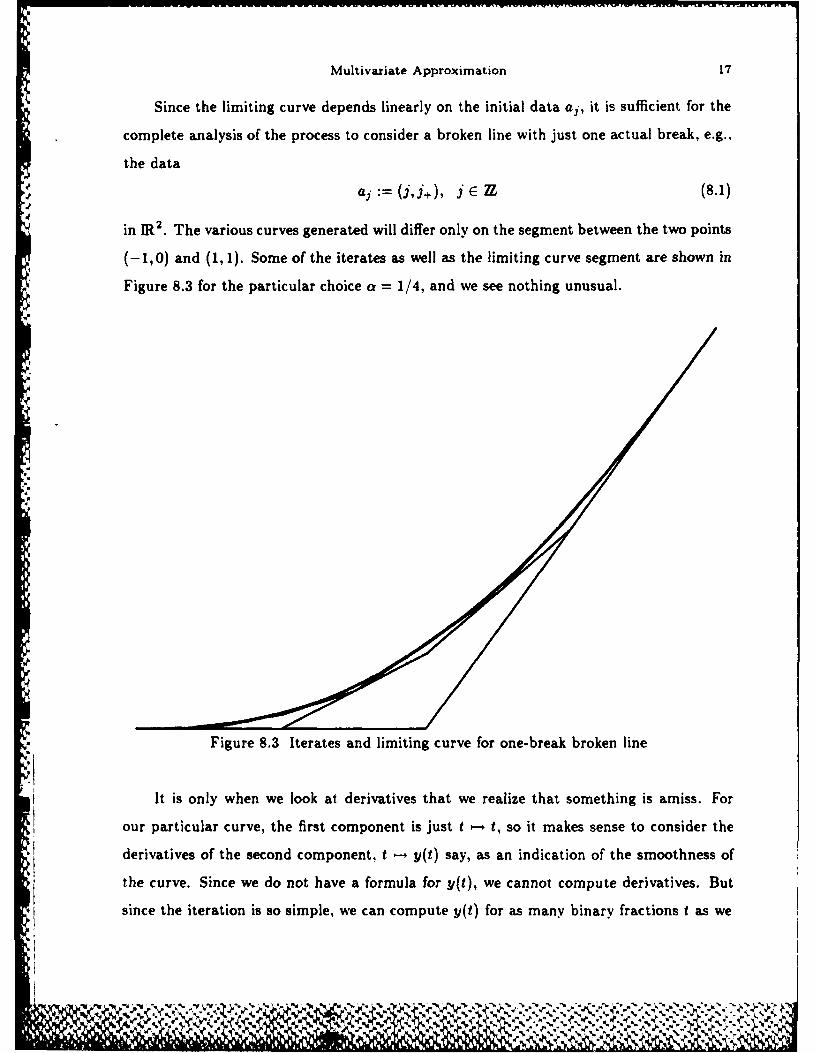
Since the limiting curve depends linearly on the initial data aj, it is sufficient for the
complete analysis of the process to consider a broken line with just one actual break, e.g..
the data
aj := (j,j+), jETI (8.1).1
in IR 2 . The various curves generated will differ only on the segment between the two points
(-1,0) and (1, 1). Some of the iterates as well as the limiting curve segment are shown in
Figure 8.3 for the particular choice a = 1/4, and we see nothing unusual.
Figure 8.3 Iterates and limiting curve for one-break broken line
It is only when we look at derivatives that we realize that something is amiss. For
our particular curve, the first component is just t - t, so it makes sense to consider the
derivatives of the second component, t - y(t) say, as an indication of the smoothness of
the curve. Since we do not have a formula for y(t), we cannot compute derivatives. But
since the iteration is so simple, we can compute y(t) for as many binary fractions t as we
'V%*1
P 4oAA 'I A~~%

18 Carl de Boor
care to. That done, we can then compute second divided differences, and these tell the
story; see Figure 8.4: The second derivative of y appears to be a fractal.
Traditional Approximation Theory views such curves with horror. There is even the
seemingly practical objection that it would be difficult to machine curves with such a
'bad' second derivative. But I do not know of experiments which have established such a
difficulty nor is it clear a priori that there should be any difficulty. On the other hand, the
generation of such curves to plotting or machining accuracy is so swift, and their flexibility
so great, that this technique is worth exploring in detail. It is this apparent local flexibility
that makes subdivision techniques a promising tool for the generation of shape-controlled
surfaces of arbitrary combinatorial structure.
* -*At*
Figure 8.4 Wisconsin WinterSecond divided differences it - h, t, t - h y plotted against 1, for
h = 2 (dots). and h 2- (stars)
For literature, see Catmull and Clark (1978). Doo (1978). and Doo And Sabin (1978). 1
am indebted to Professor Wanner for the surprising references to work by de Rham (19.17.
1953, 1956, 1957, 1959) who, many years ago and, apparently, for pedagogical reasons,
investigated a related subdivision algorithm for curves. Professor Wanner referred to it
imaginatively as 'the woodcarver's algorithm'.
4 S.,' b ' ,,, , - :~r i "'\.*-.,..,-'''- ' ' .-., ,' - .. '-.,-•":' ,.-''' .",'....P .,
Multivariate Approximation 19
References
C. de Boor (1982), Topics in Multivariate Approximation Theory, in Topics in Nu-
merical Analysis, P. Turner ed., Springer Lecture Notes in Mathematics 965, 39-78.
C. de Boor (1986), B-form basics, in Geometric Modeling, G. Farin ed., SIAM, Phila-
delphia PA, xxx-xxx.
C. de Boor ed. (1986), Approximation Theory, Amer. Mathem. Soc., Providence RI.
C. de Boor and Jia R.-q. (1985), Controlled approximation and a characterization of
the local approximation order. Proc. Amer. Math. Society 95, 547-553.
E. E. Catmull and J. H. Clark (1978), Recursively Generated B-Spline Surfaces on
Arbitrary Topological Meshes, Computer Aided Design 10, 350-353.
G. M. Chaikin (1974), An Algorithm for High Speed Curve Generation, Computer
Graphics and Image Processing 3, 346-349.
K. C. Chung and T. H. Yao (1977), On lattices admitting unique Lagrange interpo-
lations, SIAM J. Numer. Anal. 14, 735-741.
H. B. Curry and I. J. Schoenberg (1966), P61ya frequence functions.IV, The funda-
mental spline functions and their limits, J. d'Anal. Math. 17, 71-107.
W. Dahmen and C. A. Micchelli (1984), Recent Progress in Multivariate Splines, in
Approximation Theory IV, C. K. Chui, L L. Schumaker and J. Ward., eds., Academic
Press. New York, 27-121.
W. Dahmen and C. A. Micchelli (1985), On the solution of certain systems of partial
difference equations and linear independence of translates of box splines, Trans. A mer.
Math. Society 292, 305-320.
W. Dahmen and C. A. Micchelli, On the number of solutions to linear diophantine
equations and multivariate splines (1986), ms.
D. W. H. Doo (1978), A Subdivision Algorithm for Smoothing Down Irregularly
Shaped Polyhedrons, Proceedings: Interactive Techniques in Computer Aided Design,
Bologna, 157-165.
D. Doo and M. A. Sabin (1978). Behavior of Recursive Division Surfaces Near Ex-
20 Carl de Boor
traordinary Points, Computer Aided Design 6, 356-360.
G. Farin, Triangular Bernstein-Bzier patches, CAGD Report 11-1-85, Department of
Mathematics, University of Utah, Salt Lake City UT.
M. von Golitschek (1984), Shortest path algorithms for the approximation by norno-
graphic functions, in Approximation Theory and Functional Analysis, P. L. Butzer,
R. L. Stens and B. Sz.-Nagy eds, Birkhiuser Verlag, Basel, ISNM Vol. 65, xxx-xxx.
M. Golomb (1959), Approximation by functions of fewer variables, in On numerical
approximation, R. E. Langer ed., The University of Wisconsin Press, Madison WI,
275-327.
T. Grandine, The computational cost of simplex spline functions (1986), MRC TSR
#2926, U. of Wisconsin, Madison WI.
H. Hakopian (1983), Integral remainder formula of the tensor product interpolation,
Bull. Polish Acad. Sci. 31, 267-272.
K. H6llig (1986a), Box splines, in Approximation Theory V, C. K. Chui, L. L. Schu-
maker and J. Ward eds., Academic Press, xxx-xxx.
K. H61lig (1986b), Multivariate splines, in Approximation Theory, C. de Boor ed.,
Proc. Symp. Appl. Math. 36, Amer. Math. Soc. , Providence RI, 103-127.
P. Kergin (1978), Interpolation of Ck functions, Ph.D. Thesis, University of Toronto,
Canada; published as 'A natural interpolation of Ck functions' in J. Approximation
Theory 29 (1980), 278-293.
A. N. Kolmogorov (1957), On the representation of continuous functions of several
variables by superpositions of continuous functions of one variable and addition, Dok-
lady 114. 679-681.
W. A. Light and W. E. Cheney (1986), Approximation Theory in Tensor Product
Spaces, Lecture Notes in Mathematics 1169, Springer-Verlag.
G. G. Lorentz (1962). Metric entropy, widths, and superposition of functions, Ameri-
can Math. Monthly 69, 469-485.
G. G. Lorentz (1966), Approximation of Functions, Holt. Rinehart and Winston, New
York.
- - .I.V " h , ,
,,,..."..

Multivariate Approximation 21
J. Meinguet (1979). Multivariate interpolation at arbitrary points made simple,
J. Appl. Math. Phys. (ZAMP) 30, 292-304.
C. A. Micchelli (1980), A constructive approach to Kergin interpolation in JR k:mul-
tivariate B-splines and Lagrange interpolation (1980), Rocky Mountains J. Math. 10,
485-497.
C. A. Micchelli (1986), Algebraic aspects of interpolation, in Approximation Theory,C. de Boor ed., Proc. Symp. Appl. Math. 96, Amer. Math. Soc. , Providence RI,
81-102.
G. de Rhamn (1947), Un peu de mathernatique 6L propos d'une courbe plane, Elemente
der Mathematik 11, 73-76; 89-97. (Collected Works, 678-689)
-~~ C. de Rhamn (1953), Sur certaines 6quations fonctionnelles, L'otsvrage publii it 1oc casi-
on de son centenaire par l'ecole polytechnique de I'universiti de Lausanne 185S-195,
95-97. (Collected Works, 690-695)
G. de Rharn (1956), Sur une courbe plane, J. Mathem. Pures Appl. 335, 24-42. (Col-
lected Works, 696-713)
G. de Rhamn (1957), Sur quelques courbes difinies par des 6quations fonctionnelles,
Rendiconti del seminario matemnatica deli 'universitate del Politecnico di Torino 16,
101-113. (Collected Works, 714-727)
G. de Rhamn (1959), Sur les courbes limites de polygones obtenus par trisection,
lEnseignement Math. 5, 29-43. (Collected Works, 728-743)
G. Strang and G. Fix (1973), A Fourier analysis of the finite element variational
method, in Constructive Aspects of Functional Analyst's G. Geymonat ed., C.I.M.E.,
793-840.
H. Whitney (1957), On functions with bounded nth differences, J. Math. Pures App!.
36, 67-95.
% %
o-~ -Sw -. i

-" SECURITY CLASSIFICATION OF THIS PAGE (When Data Entord)
REPORT DOCUMENTATION PAGE READ INSTRUCTIONSREPORT__ DOCUMENTATIONPAGE_ BEFORE COMPLETING FORM1. REPORT NUMBER. GOVT ACCESSION NO. 3. RECIPIENT'S CATALOG NUMBER
2950 V~~4 D- A.57#4. TITLE (nd Subtitle) S. TYPE OF REPORT & PERIOD COVERED
Summary Report - no specificMULTIVARIATE APPROXIMATION reporting period
6. PERFORMING ORG. REPORT NUMBER
7. AUTHOR(s) s. CONTRACT OR GRANT NUMBER(e)
Carl de Boor DAAG9-80-C-0041
9. PERFORMING ORGANIZATION NAME AND ADDRESS 10. PROGRAM ELEMENT, PROJECT, TASKAREA & WORK UNIT NUMBERSMathematics Research Center, University of Work Unit Number 3 -
610 Walnut Street Wisconsin Numerical Analysis and
Madison, Wisconsin 53705 Scientific ComputingiS. CONTROLLIIG OFFICE NAME AND ADDRESS 12. REPORT DATE
U. S. Army Research Office August 1986P.O. Box 12211 13. NUMBER OF PAGESResearch Triangle Park, North Carolina 27709 21I MONITORING AGENCY NAME & ADDRESS(II different from Controlling Office) 1S. SECURITY CLASS. (of this report)
UNCLASSIFIED1IS&. DECLASSI FICATION/ DOWNGRADING
SCHEDULE
IS. DISTRIBUTION STATEMENT (of thlo Repo t)
Approved for public release; distribution unlimited.
17. DISTRIBUTION STATEMENT (of the abatrct entered In Block 20. If different from Report)
IS. SUPPLEMENTARY NOTES
19. KEY WORDS (Continue on revere aide if neceseey and Identify by block number)
interpolation multivariate* B- form
- .subdivision
splinesB-splines
20. ABSTRACT (Continue on reverse aide If neceeeay and Identify by block number)
The lecture addresses topics in multivariate approximation which havecaught the author's interest in the last ten years. These include: theapproximation by functions with fewer variables, correct points of polynomial
"V interpolation, the B(ernstein,-ezier,-arycentric)-form for polynomials and itsuse in understanding smooth pp functions, approximation order from spaces ofpp functions, multivariate B-splines, and surface generation by subdivision.
DD I FOR 1473 EDITION OF I NOV 65 IS OBSOLETE UNCLASSIFIEDSECURITY CLASSIFICATION OF THIS PAGE (Bmen Date Entered)
~~~ 4-4~*c&iY*~. 4

4
.J.
V
A
J..,1**
.4
4
11''S
~ -.-----