589 ' # '6& *#5 & 7 - cdn.intechopen.comcdn.intechopen.com/pdfs-wm/43454.pdf ·...

3,350+OPEN ACCESS BOOKS

108,000+INTERNATIONAL

AUTHORS AND EDITORS114+ MILLION

DOWNLOADS

BOOKSDELIVERED TO

151 COUNTRIES

AUTHORS AMONG

TOP 1%MOST CITED SCIENTIST

12.2%AUTHORS AND EDITORS

FROM TOP 500 UNIVERSITIES

Selection of our books indexed in theBook Citation Index in Web of Science™

Core Collection (BKCI)

Chapter from the book State of the Art in Biosensors - General AspectsDownloaded from: http://www.intechopen.com/books/state-of-the-art-in-biosensors-general-aspects

PUBLISHED BY

World's largest Science,Technology & Medicine

Open Access book publisher

Interested in publishing with IntechOpen?Contact us at [email protected]

http://www.intechopen.com/books/state-of-the-art-in-biosensors-general-aspects

mailto:[email protected]

Chapter 11

Love Wave Biosensors: A Review

María Isabel Rocha Gaso, Yolanda Jiménez,Laurent A. Francis and Antonio Arnau

Additional information is available at the end of the chapter

http://dx.doi.org/10.5772/53077

1. Introduction

In the fields of analytical and physical chemistry, medical diagnostics and biotechnologythere is an increasing demand of highly selective and sensitive analytical techniques which,optimally, allow an in real-time label-free monitoring with easy to use, reliable, miniatur‐ized and low cost devices. Biosensors meet many of the above features which have led themto gain a place in the analytical bench top as alternative or complementary methods for rou‐tine classical analysis. Different sensing technologies are being used for biosensors. Catego‐rized by the transducer mechanism, optical and acoustic wave sensing technologies haveemerged as very promising biosensors technologies. Optical sensing represents the most of‐ten technology currently used in biosensors applications. Among others, Surface PlasmonResonance (SPR) is probably one of the better known label-free optical techniques, being themain shortcoming of this method its high cost. Acoustic wave devices represent a cost-effec‐tive alternative to these advanced optical approaches [1], since they combine their direct de‐tection, simplicity in handling, real-time monitoring, good sensitivity and selectivitycapabilities with a more reduced cost. The main challenges of the acoustic techniques re‐main on the improvement of the sensitivity with the objective to reduce the limit of detec‐tion (LOD), multi-analysis and multi-analyte detection (High-Throughput Screeningsystems-HTS), and integration capabilities.

Acoustic sensing has taken advantage of the progress made in the last decades in piezoelec‐tric resonators for radio-frequency (rf) telecommunication technologies. The so-called gravi‐metric technique [2], which is based on the change in the resonance frequency experimentedby the resonator due to a mass attached on the sensor surface, has opened a great deal ofapplications in bio-chemical sensing in both gas and liquid media.

© 2013 Gaso et al.; licensee InTech. This is an open access article distributed under the terms of the CreativeCommons Attribution License (http://creativecommons.org/licenses/by/3.0), which permits unrestricted use,distribution, and reproduction in any medium, provided the original work is properly cited.

Traditionally, the most commonly used acoustic wave biosensors were based on QCM devi‐ces. This was primarily due to the fact that the QCM has been studied in detail for over 50years and has become a mature, commercially available, robust and affordable technology[3, 4]. LW acoustic sensors have attracted a great deal of attention in the scientific communi‐ty during the last two decades, due to its reported high sensitivity in liquid media comparedto traditional QCM-based sensors. Nevertheless, there are still some issues to be further un‐derstood, clarified and/or improved about this technology; mostly for biosensor applica‐tions.

LW devices are able to operate at higher frequencies than traditional QCMs [5]; typical oper‐ation frequencies are between 80-300 MHz. Higher frequencies lead, in principle, to highersensitivity because the acoustic wave penetration depth into the adjacent media is reduced[6]. However, the increase in the operation frequency also results in an increased noise level,thus restricting the LOD. The LOD determines the minimum surface mass that can be de‐tected. In this sense, the optimization of the read out and characterization system for thesehigh frequency devices is a key aspect for improving the LOD [7].

Another important aspect of LW technology is the optimization of the fluidics, specially theflow cell. This is of extreme importance for reducing the noise and increasing the biosensorsystem stability; aspects that will contribute to improve the LOD.

The analysis and interpretation of the results obtained with LW biosensors must be deeperunderstood, since the acoustic signal presents a mixed contribution of changes in the massand the viscoelasticity of the adsorbed layers due to interactions of the biomolecules. A bet‐ter understanding of the transduction mechanism in LW sensors is a first step to advance inthis issue; however its inherent complexity leads, in many cases, to frustration [8].

The fabrication process of the transducer, unlike in traditional QCM sensors, is another as‐pect under investigation in LW technology, where features such as: substrate materials,sizes, structures and packaging must be still optimized.

This chapter aims to provide an updated insight in the mentioned topics focused on biosen‐sors applications.

2. Basis of LW sensors

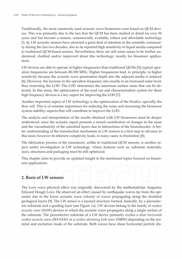
The Love wave physical effect was originally discovered by the mathematician AugustusEdward Hough Love. He observed an effect caused by earthquake waves far from the epi‐center due to the lower acoustic wave velocity of waves propagating along the stratifiedgeological layers [9]. The LW sensor is a layered structure formed, basically, by a piezoelec‐tric substrate and a guiding layer (see Figure 1a). LW devices belong to the family of surfaceacoustic wave (SAW) devices in which the acoustic wave propagates along a single surface ofthe substrate. The piezoelectric substrate of a LW device primarily excites a shear horizontalsurface acoustic wave (SH-SAW) or a surface skimming bulk wave (SSBW) depending on the ma‐terial and excitation mode of the substrate. Both waves have shear horizontal particle dis‐

State of the Art in Biosensors - General Aspects278

placements (perpendicular to the wave propagation direction and parallel to the waveguidesurface). This type of acoustic wave operates efficiently in liquid media, since the radiationof compressional waves into the liquid is minimized.

Guiding layerIDTs

Propagation direction

Particle displacement

Sensing area

Piezoelectric substratePiezoelectric substrate

(semi-infinite)

Guiding layerSensing area

Fluid medium(semi-infinite)

d

l

μF , ρF , ηF

μSA , ρSA , ηSA

μL , ρL , ηL

μS , ρS , ηS

a) b)

y

z

y

z x

Coating μC , ρC , ηC h

Figure 1. a) Basic structure of a LW sensor. b) Five-layer model of a LW biosensor.

LW sensors consist of a transducing area and a sensing area. The transducing area consistsof the interdigital transducers (IDTs), which are metal electrodes, sandwiched between thepiezoelectric substrate and the guiding layer. The input IDT is excited electrically (applyingan rf signal) and launches a mechanical acoustic wave into the piezoelectric material whichis guided through the guiding layer up to the output IDT, where it gets transformed back toa measurable electrical signal. The sensing area is the area of the sensor surface, located be‐tween the input and output IDT, which is exposed to the analyte.

LW sensors can be used for the characterization of processes involving several layers de‐posited over the sensing area; such is the case of biosensors. A LW biosensor can be descri‐bed as a layered compound formed by the LW sensor in contact with a finite viscoelasticlayer, the so-called coating, contacting a semi-infinite viscoelastic liquid as indicated in Fig‐ure 1b. Each layer has its material properties given by: the shear modulus μ, density ρ andviscosity η. Hence, the subscripts S, L, SA, C and F denotes the substrate, guiding layer,sensing area, coating and fluid layers, respectively. Biochemical interactions at the sensingarea cause changes in the properties of the propagating acoustic wave which can be detect‐ed at the output IDT.

The difference between the mechanical properties of the guiding layer and the substrate cre‐ates an entrapment of the acoustic energy in the guiding layer keeping the wave energy nearthe surface and slowing down the wave propagation velocity. This guiding layer phenom‐enon makes LW devices very sensitive towards any changes occurring on the sensor surface,

Love Wave Biosensors: A Reviewhttp://dx.doi.org/10.5772/53077

279

such as those related to mass loading, viscosity and conductivity [5]. The higher the confine‐ment of the wave in the guiding layer, the higher the sensitivity [10].

The proper design of a LW device for biosensor applications must consider the advancesmade on these basic elements. Updated information about each one of these elements is thenrequired and can be found in the following sections.

2.1. Piezoelectric substrate

Thanks to piezoelectricity electrical charges can be generated by the imposition of mechanicalstress. The phenomenon is reciprocal; applying an appropriate electrical field to a piezoelec‐tric material generates a mechanical stress [11]. In LW sensors an oscillating electric field (rfsignal) is applied in the input IDT which, due to the piezoelectric properties of the substrate,launches an acoustic guided wave. The guided wave propagates through the guiding layerup to the output IDT where, again due to the piezoelectric properties of the substrate, is con‐verted back to an electric field for measurement. A remarkable parameter of the piezoelec‐tric substrate is the electromechanical coupling coefficient (K2), which indicates the conversionefficiency from electric energy to mechanical energy; its value depends on the material prop‐erties. This is an important design parameter in LW sensors, since higher K2 lead to low lossLW devices and, therefore, more sensitive LW sensors [12].

When choosing a material for the substrate of LW devices, apart from the desired low losses,other requirements, such as low temperature coefficient of frequency (TCF) have to be consid‐ered as well. Special crystal cuts of the piezoelectric substrate material1 can yield an intrinsi‐cally temperature-compensated device which minimizes the influence of temperature on thesensor response, thus improving the LOD [13,14].

The shear horizontal polarization required for operation of the LW sensor in liquid media isanother aspect to be considered when choosing the substrate material. In this sense, quartzis the only common substrate material that can be used to obtain a purely shear polarizedwave [13]. The crystal cut and the wave propagation direction, which depends on the IDTsorientation, define the elastic, dielectric and piezoelectric constants of the crystal, and there‐fore the wave polarization. Possible cuts which generate a purely shear polarized wave arethe AT-cut quartz and the ST-cut quartz. AT-cut quartz and ST-cut quartz are both Y-cuts,rotated 35°15’ and 42°45° about the original crystallographic X-axis, respectively.

Initially, LW devices were made in ST-cut quartz [15], however, ST-cut quartz is very sensi‐tive to temperature (its TCF is around 40 ppm/°C) [16]. This was a restrictive factor in termsof sensor LOD and, thus, temperature-compensated systems based on different quartz cutsand different materials for the substrate such as lithium tantalate (LT), LiTaO3, and lithiumniobate (LN), LiNbO3, were investigated [17-19]. In particular, AT-cut quartz, 36° YX LT and36° YX LN were proposed, the last two corresponds to specific cuts of LT and LN materials[10]. Table 1 contains the values of some characteristic parameters of the previously men‐

1 The substrate crystal cuts (or plates) are obtained by cutting slices of a single-crystal starting material with an arbitra‐ry orientation relative to the three orthogonal crystallographic axes.


tioned substrate materials. In column 2, the substrate shear velocity vS, is defined by the sub‐strate material properties (vS = (μS/ρS)1/2).

Substrate vS (m/s) ρS(kg/m3) K2 (%) TCF (ppm/°C)

ST-cut Z’ propagating quartz 5050 2650 1.9 40

AT-cut Z’ propagating quartz 5099 2650 1.4 0-1

36° YX LN 4800 4628 16 -75 to -80*

36° YX LT 4200 7454 5 -30 to -45

Table 1. Most commonly employed crystal cuts for LW devices (modified from [18]).*Approximate value.

LN substrates have higher coupling factor and low propagation loss than LT and quartzsubstrates. However, these substrates are extremely vulnerable to abrupt thermal shocks.

The low insertion loss, very large electromechanical coupling factor K2 and low propagationloss which characterize 36° YX LT substrates [20] provide advantages over other substratessuch as quartz cuts, where exquisite care in the fluidic packaging is required to prevent ex‐cessive wave damping [21]. For this reason, LT seems to be the substrate material of choicein high-loss applications due to its high coupling factor K2, while in low-loss applicationsquartz may exhibit better wave characteristic [22]. The main shortcomings of 36° YX LT sub‐strates are: they do not generate a pure shear wave, which increases the damping when isliquid loaded; and they have a poor thermal stability due to their high TFC (-30 to -40ppm/°C [19]) if compared with AT-quartz.

From the point of view of thermal stability, AT-cut quartz seems to be the most appropriatedue to its very low TCF [14]. Although the coupling coefficient of the AT-cut quartz is thelowest compared to other cuts, in our opinion, AT-cut quartz is currently the most suitablesubstrate for LW biosensing applications among the mentioned substrates, for several rea‐sons: 1) it is capable of generating pure shear waves, diminishing the damping when is liq‐uid loaded; 2) its thermal stability is the highest one, which improves the LOD; 3) the masssensitivity of quartz substrates is significantly high than that of LT substrates [17,23]; and 4)LT and LN substrates are extremely fragile and must be handled with great care during thedevice fabrication to prevent them from breaking in pieces.

2.2. Interdigital transducers

Interdigital transducers (IDTs) were firstly reported in 1965 by White and Voltmer [24] forgenerating SAWs in a piezoelectric substrate. An IDT, in its most simple version, is formedby two identical combs-like metal electrodes whose strips are located in a periodic alternat‐ing pattern located on top of the piezoelectric substrate surface. Figure 2a shows the struc‐ture of a single-electrode IDT which consists of two strips per period p and acoustic aperture W.The strip width is equal to the space between strips (p/4). One comb is connected to ground


281

and the other to the center conductor of a coaxial cable where a rf signal is provided. A pairof two strips with different potential is called a finger pair.

The IDT electric equivalent circuit is explained in reference [25]. Figure 2b shows the IDTfrequency response, where A(f) is the electrical amplitude of the rf signal. The maximum inA(f) occurs when the wavelength λ of the generated acoustic wave is equal to the period pand this arises at the so called synchronous frequency fs. In relation to the bandwidth B of anIDT frequency response, this will be narrower when increasing the number of finger pairs N.However, there is a limitation in the maximum N recommended, due to the fact that, inpractice, when N exceeds 100, the losses associated with mass loading and the scatteringfrom the electrodes increase. This neutralizes any additional advantage associated with theincrease of the number of the finger pairs.

Due to symmetry of the IDT in the direction of propagation, the LW energy is emitted inequal amounts in opposite directions, giving an inherent loss of 3 dB. In a two-port devicethis factor contributes 6 dB to the total insertion loss [25,26].

Aluminum has been widely used as IDTs material and has been extensibility demonstratedin literature as suitable for SAW generation. Aluminum has an ability to resist corrosion andis the third most abundant element on Earth (after oxygen and silicon). It also has a low costcompared to other metals. The metallic layer of the electrodes must be thick enough topresent a low electric resistance, but sufficiently thin to avoid an excessive mechanic chargefor the acoustic wave (acoustic impedance breaking) [27]. Generally, a thickness between100 and 200 nm of aluminum is employed.

There are a number of second-order effects, which are often significant in practice, that af‐fect the transducer frequency response. The effect for which the transducer strips reflect sur‐face waves causing mechanical and electrical perturbations of the surface is called electrodeinteraction [30]. Usually, these unwanted reflections cancel each other over wide frequencybands and become negligible. However, in a certain frequency band, the scattered waves arein phase, adding them constructively and causing very strong reflection (Bragg reflection)which distorts the transducer frequency response. For a single-electrode IDT (see Figure 2a),this situation occurs at the resonance condition λ = p. Thus, double-electrode (or double fingerpair or split-electrode) IDTs are used to avoid this unwanted effect. In double-electrode IDTsthere are four strips per period (see Figure 2c) and thus, the Bragg reflection can be sup‐pressed at the LW resonance frequency [28]. One disadvantage of the double-electrode is theincreased lithographic resolution required for fabricating the IDTs [29].

Another significant second-order effect is the generation of the triple-transit signal. In a de‐vice using two IDTs, which is the case of a LW device, the output IDT will in general pro‐duce a reflected wave, which is then reflected a second time by the input IDT. Thus, areflected wave reaches the output IDT after traversing the substrate three times, giving anunwanted output signal known as the triple-transit signal [26]. This effect is reduced by mak‐ing the input and output IDT separation large enough.

Some authors use reflectors to improve the frequency response of the LW device. Reflectorsare composed of metal gratings placed in the same configuration than IDTs and are located


at the ends of the IDTs (see Figure 2d). These components have generally less finger pairsthan the IDTs. The space periodicity of the reflectors is equal than in the IDTs [30]. Very nar‐row low-loss pass band can be realized in a two-port device, when the device is designed sothat the reflectors resonate at the IDT resonance frequency, since the transfer admittance be‐comes very large [28].

2.3. Guiding layer

The difference between the mechanical properties of the piezoelectric substrate and theguiding layer generates a confinement of the acoustic energy in the guiding layer, slowingdown the wave propagation velocity, but maintaining the propagation loss [32]. In particu‐lar, the condition for the existence of Love wave modes is that the shear velocity of the guid‐ing layer material (vL = (μL/ρL)1/2) is less than that of the substrate (vS = (μS/ρS)1/2) [31]. Whenboth materials, substrate and guiding layer, have similar density the ratio μS/ μL determinethe dispersion of the Love mode; a large value of that ratio (higher μS and lower μL) leads toa stronger entrapment of the acoustic energy [32] and thus, greater sensitivity. Hence, thebenefit of the guiding layer is that an enhanced sensitivity to mass deposition can be ob‐tained [33], but also to viscoelastic interactions.

Running Title 5

shear wave, which increases the damping when is liquid loaded; and they have a poor thermal 1 stability due to their high TFC (-30 to -40 ppm/°C [19]) if compared with AT-quartz. 2

From the point of view of thermal stability, AT-cut quartz seems to be the most appropriate due to its 3 very low TCF [14]. Although the coupling coefficient of the AT-cut quartz is the lowest compared to 4 other cuts, in our opinion, AT-cut quartz is currently the most suitable substrate for LW biosensing 5 applications among the mentioned substrates, for several reasons: 1) it is capable of generating pure 6 shear waves, diminishing the damping when is liquid loaded; 2) its thermal stability is the highest 7 one, which improves the LOD; 3) the mass sensitivity of quartz substrates is significantly high than 8 that of LT substrates [17,23]; and 4) LT and LN substrates are extremely fragile and must be handled 9 with great care during the device fabrication to prevent them from breaking in pieces. 10

2.2. Interdigital transducers 11

Interdigital transducers (IDTs) were firstly reported in 1965 by White and Voltmer [24] for 12 generating SAWs in a piezoelectric substrate. An IDT, in its most simple version, is formed by two 13 identical combs-like metal electrodes whose strips are located in a periodic alternating pattern located 14 on top of the piezoelectric substrate surface. Figure 2a shows the structure of a single-electrode IDT 15 which consists of two strips per period p and acoustic aperture W. The strip width is equal to the 16 space between strips (p/4). One comb is connected to ground and the other to the center conductor of 17 a coaxial cable where a rf signal is provided. A pair of two strips with different potential is called a 18 finger pair. 19

The IDT electric equivalent circuit is explained in reference [25]. Figure 2b shows the IDT frequency 20 response, where A(f) is the electrical amplitude of the rf signal. The maximum in A(f) occurs when the 21 wavelength λ of the generated acoustic wave is equal to the period p and this arises at the so called 22 synchronous frequency fs. In relation to the bandwidth B of an IDT frequency response, this will be 23

a) b)A(f)

f

B

p

p/8

W

c)

p p p pd)

Reflectors

fs

W

p/4

p

Figure 2. a) Single-electrode Interdigital Transducer (IDT) with period p, electrode width equal to space between electrodes (p/4) and aperture W (modified from [25]). b) Frequency response of an IDT (positive frequencies), where A(f) is the electrical amplitude (modified from [25]). c) Double-electrode IDT with period p, electrode width equal to space between electrodes and aperture W. d) Two grating reflectors are place at both ends of the IDTs (modified from [30]).

Figure 2. a) Single-electrode Interdigital Transducer (IDT) with period p, electrode width equal to space between elec‐trodes (p/4) and aperture W (modified from [25]). b) Frequency response of an IDT (positive frequencies), where A(f) isthe electrical amplitude (modified from [25]). c) Double-electrode IDT with period p, electrode width equal to spacebetween electrodes and aperture W. d) Two grating reflectors are place at both ends of the IDTs (modified from [30]).


283

The effect of the guiding layer on Love modes influence the substrate coupling factor K2, in‐creasing it [14]. Also influence the temperature behavior, since modifies the TCF comparedto their parent SSBWs device.

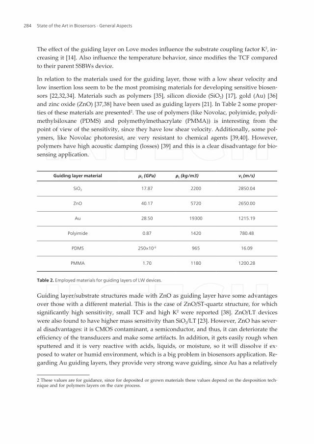
In relation to the materials used for the guiding layer, those with a low shear velocity andlow insertion loss seem to be the most promising materials for developing sensitive biosen‐sors [22,32,34]. Materials such as polymers [35], silicon dioxide (SiO2) [17], gold (Au) [36]and zinc oxide (ZnO) [37,38] have been used as guiding layers [21]. In Table 2 some proper‐ties of these materials are presented2. The use of polymers (like Novolac, polyimide, polydi‐methylsiloxane (PDMS) and polymethylmethacrylate (PMMA)) is interesting from thepoint of view of the sensitivity, since they have low shear velocity. Additionally, some pol‐ymers, like Novolac photoresist, are very resistant to chemical agents [39,40]. However,polymers have high acoustic damping (losses) [39] and this is a clear disadvantage for bio‐sensing application.

Guiding layer material μL (GPa) ρL (kg/m3) vL (m/s)

SiO2 17.87 2200 2850.04

ZnO 40.17 5720 2650.00

Au 28.50 19300 1215.19

Polyimide 0.87 1420 780.48

PDMS 250×10-6 965 16.09

PMMA 1.70 1180 1200.28

Table 2. Employed materials for guiding layers of LW devices.

Guiding layer/substrate structures made with ZnO as guiding layer have some advantagesover those with a different material. This is the case of ZnO/ST-quartz structure, for whichsignificantly high sensitivity, small TCF and high K2 were reported [38]. ZnO/LT deviceswere also found to have higher mass sensitivity than SiO2/LT [23]. However, ZnO has sever‐al disadvantages: it is CMOS contaminant, a semiconductor, and thus, it can deteriorate theefficiency of the transducers and make some artifacts. In addition, it gets easily rough whensputtered and it is very reactive with acids, liquids, or moisture, so it will dissolve if ex‐posed to water or humid environment, which is a big problem in biosensors application. Re‐garding Au guiding layers, they provide very strong wave guiding, since Au has a relatively

2 These values are for guidance, since for deposited or grown materials these values depend on the desposition tech‐nique and for polymers layers on the cure process.


low shear acoustic velocity and a high density. However, it couples the rf signal from inputto output IDT.

Silicon dioxide (SiO2) -also known as fused silica- is a standard material in semiconductorindustry and offers low damping, sufficient low shear velocity and excellent chemical andmechanical resistance [41]. It is the only native oxide of a common semiconductor which isstable in water and at elevated temperatures, an excellent electrical insulator, a mask to com‐mon diffusing species, and capable of forming a nearly perfect electrical interface with itssubstrate. When SiO2 is needed on materials other than silicon, it is obtained by chemical va‐por deposition (CVD), either thermal CVD or Plasma enhanced CVD (PECVD) [42]. Themain shortcoming for SiO2 is that the optimum thickness, at which the maximum sensitivityis reached, is very high (see Section 5), so this complicates the manufacturing process. Nev‐ertheless, at the present, we consider that SiO2 is the most appropriate material for LW bio‐sensors guiding layer, mainly due to its low damping and excellent chemical andmechanical properties [42].

2.4. Sensing area

The sensing area can be made of different material than the guiding layer. Sensing layershave been reported composed of materials like PMMA [43] and SU-8 [44], but the most com‐monly employed is gold (Au). Generally, the thickness of this layer varies from 50-100 nmand 2-10 nm of chrome (Cr) or titanium (Ti) is needed to promote adherence to the guidinglayer. Au surfaces are very attractive candidates for self-assembly due to their metallic na‐ture, great nobility, and particular affinity for sulphur. This aspect allows functionalizationwith thiols of various types and adhesion to diverse organic molecules, which are modifiedto contain a sulphur atom. These coatings, assembled onto the gold surfaces, can serve asbiosensors [36]. Immobilization techniques on gold for biosensing are quite common andmuch utilized in the scientific community. However, immobilization techniques on differentmaterials, like SiO2, could greatly simplify the LW biosensors fabrication.

3. Measurement techniques

Figure 3a shows a configuration of a two-port LW device where it behaves as a delayline. D is the distance between input and output IDT and L is the center-to-center dis‐tance between the IDTs. Thus, the sensor is a transmission line which transmits a mechan‐ical signal (acoustic wave) launched by the input port (input IDT) due to the applied rfelectrical signal. After a time delay the traveling mechanical wave is converted back to anelectric signal in the output port (output IDT). In general, changes in the coating layerand/or in the semi-infinite fluid medium (see Figure 1b) produce variations in the acous‐tic wave properties (wave propagation velocity, amplitude or resonant frequency). Thesevariations can be measured comparing the input and output electrical signal, since pha‐sor Vin remains unchanged, while phasor Vout changes. Thus, from an electric point ofview, a LW delay line can be defined by its transfer function H(f) = Vout/Vin, which repre‐


285

sents the relationship between input and output electrical signal. H(f) is a complex num‐ber which can be defined as H(f) = Aejφ, being A = |Vout/Vin| the amplitude and φ the phaseshift between Vout and Vin. In terms of voltage, the insertion loss (IL) in dB is given by 20log10(A). Figure 3b, presents the frequency response of an AT-cut Z’ propagating/SiO2 LWdevice designed a fabricated by the authors of this chapter.

Figure 3. a) Scheme of a LW delay line. It consists of two ports. In the input IDT an rf signal is applied which launchesan acoustic propagating wave. The output signal is recorded at the output IDT. D is the distance between input andoutput IDT and L is the center-to-center distance between the IDTs. b) Frequency response of a LW device designed afabricated by the authors of this chapter. The phase shift (dotted line) and IL (solid line) were measured using a net‐work analyzer.

In biosensors, biochemical interactions at the sensing area will modify the thickness andproperties of the coating, and therefore variations in the amplitude and phase of the electri‐cal transfer function can be measured. These variations can be monitored in real time, whichprovides valuable information about the interaction process.

The LW delay line can be used as frequency determining element of an oscillator circuit(closed loop configuration). Effectively, in an oscillator circuit the LW device is placed as a de‐lay line in the feedback loop of an rf amplifier in a closed loop configuration [10,45]. There‐fore, a change in the wave velocity, due to a sensing effect, produces a time delay in thesignal through the LW device which appears as phase-shift; this phase-shift is transferred interms of frequency-shift in an oscillator configuration. The oscillator is, apparently, the sim‐plest electronic setup: the low cost of their circuitry as well as the integration capability andcontinuous monitoring are some features which make the oscillators an attractive configura‐tion for the monitoring of the determining parameter of the resonator sensor, which in thecase of the LW device is the phase-shift of the signal at resonance [46-49]. However, due tothe following drawbacks, in our opinion, the oscillators are not the best option for acousticwave sensor characterization: 1) they do not provide direct information about signal ampli‐tude; 2) they, eventually, can stop oscillation if insertion losses exceed the amplifier gainduring an experiment; and 3) despite of the apparent simple configuration, a very good de‐sign is necessary to guarantee that a LW resonator will operate at a specific frequency, andthis is not a simple task. In effect, in the same way than in QCM oscillators it is required toassure that the sensor resonates on one defined resonance mode and does not “jump” be‐


tween spurious resonances [7], in LW oscillators one must assure that the sensor will oper‐ate at one phase ramp in the sensor response band-pass, and does not jump from one toanother which are almost of identical characteristics (see Figure 3b). Moreover, when theresonator dimensions get smaller and the frequency increases this becomes more difficult toachieve, since when increasing frequency there is a decrease of the resonator quality factor, adecrease in frequency stability [50] and in LW the ramps become nearer to each other.

In an open loop configuration, the input transducer is excited at a fixed frequency while thephase shift between Vout and Vin, φ, is recorded [32]. In this configuration, in the absence ofinterferences, phase variations measured experimentally can be related to changes in thephysical properties of the layers deposited over the sensing area.

Network analyzers are the most commonly used instrumentation for characterizing LW de‐lay lines in open loop configurations. Nevertheless, recently, some authors successfully vali‐dated a new characterization technique based on the open loop configuration [51]. A readout circuit based on this technique for high frequency liquid loaded QCM devices has beendeveloped by the same authors [52], and tested with LW devices with very satisfactory re‐sults [53]. The main advantages of this read out circuit are its low cost, high integration,small size, calibration facility and the possibility of being used as an interface for multi-anal‐ysis detection.

4. Modeling methods

As mentioned, there is an open research field regarding the employed materials, and itsphysical and geometric properties for achieving more optimized LW devices for biosensorsapplications. For instance, the thickness of the Love-wave guiding layer is a crucial parame‐ter that can be varied to achieve a more sensitivity device. The fabrication of LW sensors iscomplex and expensive due to their micro sizes [54]; therefore, simulations and modeling ofLW devices as previous steps to their production could be very valuable. Models allow re‐lating changes in some characteristics of the wave, as the velocity, with changes in the physi‐cal properties of the layers deposited over the sensing area, and thus, provide informationabout the sensing event. Nevertheless, modeling LW devices commonly requires simplifiedassumptions or the use of numerical methods [23] due to the complex nature of SAW propa‐gation in anisotropic and piezoelectric materials.

In this section, information regarding the current most popular models used for modelingLW sensors is provided: the transmission line model, the dispersion equation and the FiniteElement Method.

4.1. Transmission line model

It is well known that the propagation and attenuation of acoustic waves in guiding struc‐tures can be obtained by equivalent transmission line models [8,55]. The theory of soundwave propagation is very similar mathematically to that of electromagnetic waves, so tech‐


287

niques from transmission line theory are also used to build structures to conduct acousticwaves; and these are also called transmission lines. The transmission line model (TLM) foracoustic waves take advantage of the concepts and techniques of proven value in electro‐magnetic microwaves to corresponding problems in elastic guided waves [8].

A transmission line is characterized by its secondary parameters which are the propagationwavevector k (when scalar wavenumber) and the characteristic impedance Zc (see Figure 4a). It isimportant to mention that these parameters do not depend on the transmission line length.In each plane of an electric transmission line it is possible to define a magnitude for a volt‐age and other for the current in the line. For acoustics transmission lines current and voltagein electromagnetic are replaced by the particle velocity vp and the stress -TJ, respectively,where J indicates de stress direction (J = 1, 2,..., 6) [55]. In an acoustic transmission line Zc

represents the relation between the stress -TJ and the particle velocity vp of the material, andk quantifies how the wave energy will be propagated along the transmission line. To quanti‐fy the variations of -TJ and vp when the wave propagates through the transmission line, thelumped elements models presented in Figure 4b and 4c are introduced. Figure 4b corre‐sponds to the series model, and Figure 4c to the parallel model. The lumped elements ofthese models are called the transmission line primary parameters, which are dependent on theline length. Analyzing the parallel model of Figure 4c, the following coupled differentialequations are obtained:

2

2

2

2

Jp

pJ

d TZ Y v

drd v

Z Y Tdr

= × ×

= × ×

(1)

where Z=jωL, Y=G+jωC and ω=2πf. Being Z, L, Y, C, G, f, the impedance, inductance, admit‐tance, capacitance and conductance per unit of length, respectively and f the frequency of TJ

and vp.

The solutions for these equations are given by:

Book Title 10

C dr

L/2 dr L/2 dr

G dr

vp

r r + dr

+

-

TJ

a)

k, ZcTJ (r,t)

vp (r,t)

r r + dr

b)b.2)

C dr

L dr

G dr

vp

r r + dr

TJ

+

-

vp (r,t)

TJ (r,t)

r r + dr

L/2 dr L/2 dr

C dr

G dr

c)

TJ (r,t)

vp (r,t) L dr

C dr G dr

r r + dr

Figure 4. a) Pictorial representation of a transmission line. b) Transmission line equivalent series model for acoustic propagation in a viscoelastic layer. c) Transmission line equivalent parallel model for acoustic propagation in a viscoelastic layer.

4.1. Transmission line model 1

It is well known that the propagation and attenuation of acoustic waves in guiding structures can be 2 obtained by equivalent transmission line models [8,55]. The theory of sound wave propagation is very 3 similar mathematically to that of electromagnetic waves, so techniques from transmission line theory 4 are also used to build structures to conduct acoustic waves; and these are also called transmission 5 lines. The transmission line model (TLM) for acoustic waves take advantage of the concepts and 6 techniques of proven value in electromagnetic microwaves to corresponding problems in elastic 7 guided waves [8]. 8

A transmission line is characterized by its secondary parameters which are the propagation 9 wavevector k (when scalar wavenumber) and the characteristic impedance Zc (see Figure 4a). It is 10 important to mention that these parameters do not depend on the transmission line length. In each 11 plane of an electric transmission line it is possible to define a magnitude for a voltage and other for 12 the current in the line. For acoustics transmission lines current and voltage in electromagnetic are 13 replaced by the particle velocity vp and the stress -TJ, respectively, where J indicates de stress 14 direction (J = 1, 2, ..., 6) [55]. In an acoustic transmission line Zc represents the relation between the 15 stress -TJ and the particle velocity vp of the material, and k quantifies how the wave energy will be 16 propagated along the transmission line. To quantify the variations of -TJ and vp when the wave 17 propagates through the transmission line, the lumped elements models presented in Figure 4b and 4c 18 are introduced. Figure 4b corresponds to the series model, and Figure 4c to the parallel model. The 19 lumped elements of these models are called the transmission line primary parameters, which are 20 dependent on the line length. Analyzing the parallel model of Figure 4c, the following coupled 21 differential equations are obtained: 22

2

2

2

2

Jp

pJ

d TZ Y v

dr

d vZ Y T

dr

(0.1) 23

where Z=jωL, Y=G+jωC and ω=2π/f. Being Z, L, Y, C, G, f, the impedance, inductance, admittance, 24 capacitance and conductance per unit of length, respectively and f the frequency of TJ and vp. 25

The solutions for these equations are given by: 26

( )

( )

r rJ J J

r rJ Jp

c c

T r T e T e

T Tv r e e

Z Z

(0.2) 27

Figure 4. a) Pictorial representation of a transmission line. b) Transmission line equivalent series model for acousticpropagation in a viscoelastic layer. c) Transmission line equivalent parallel model for acoustic propagation in a viscoe‐lastic layer.


( )

( )

r rJ J J

J Jr rp

c c

T r T e T e

T Tv r e e

Z Z

g g

g g

+ - × - ×

+ -- × ×

= +

= -

r r

r r

r

r (2)

where T+ and T- are arbitrary values for the intensity of the incident an reflected waves, re‐spectively. The linear propagation exponent or complex propagation factor γ is directly related tothe wavevector (γ=jk) and is given by γ = (ZY)1/2 = α + jβ. The real part of γ, denoted as at‐tenuation coefficient α, represents the attenuation suffered by the wave when propagatingthrough the transmission line. The imaginary part of γ, denoted as phase coefficient β, whenmultiplied by a distance, quantifies the phase shift that the wave suffers when traveling thatdistance. The characteristic impedance of the line Zc is given by Zc=(Z/Y)1/2. First row of Ta‐ble 3 shows the relationship between primary and secondary parameters of a transmissionline for the series and parallel model.

The relation between the secondary (or primary) parameters and the properties of the trans‐mission line materials is achieved by comparing Eqs. (1) with the motion equations of theLW assuming isotropic layers [55]. These relations are given in the second row of Table 3 forthe series and parallel model.

Series model Parallel model

k = − jγ=ω LC1 + jωC / G

Zc = LC + jω L

G

k = − jγ= − j jωL (G + jωC)

Zc = jωLG + jωC

C = 1μ

G = 1η

L =ρ

C = μω 2η 2 + μ 2

G = ηω 2

ω 2η 2 + μ 2

L =ρ

Table 3. Equivalent transmission line model parameters in terms of the layer properties.

Figure 5a shows a simplify description in which a LW propagates in a waveguide structure.Two assumptions were made: 1) the materials in the figure are isotropic (for piezoelectricsubstrates this assumption is valid because of a low anisotropy) and 2) the main wave prop‐agating in the z direction results from the interaction of two partial waves with the samecomponent in z direction and opposites components in y direction [12].

If all the properties of the layers which are involved in the LW transmission line areknown, it is possible to obtain the phase velocity of the Love mode vφ. The LW propagates ineach layer i of the device in two directions z and y. In the case of a typical biosensor the de‐vice consists of 5 layers with the subscripts i equal to: S for the substrate, L for the guidinglayer, SA for the sensing area, C for the coating and F for the fluid. Direction z is known asthe longitudinal direction and direction y as the transverse direction. The wave does not find


289

any material properties change in the longitudinal direction; hence it propagates in this di‐rection acquiring a phase shift and attenuation (in case of material with losses). However,in the transverse direction a stationary wave exists when the resonance condition is met.Thus, each layer counts with two transmission lines, one in the transverse direction and theother in the longitudinal direction. When a wave propagates in y’ direction (see Figure 5a),as it happens with the partial waves of a layer i, ki has that same direction (see Figure 5b),and therefore, it has components in z and y directions. In this way, the secondary parame‐ters of each transmission line are determined from the projection of the parameter in theproper direction. The relation between the wavevector and the wave velocity is ki=ω/vi.Therefore, ki and vi have the same directions, so the wave velocity in y’ direction also hascomponents in z and y.

Equations (3) and (4) give the expression of the secondary parameters and wave velocity inthe transverse and longitudinal directions, respectively:

cos , cos , cosciy ci i iy i i iy i iZ Z k k v vq q q= = = (3)

sin , sin , sinciz ci i iz i i iz i iZ Z k k v vq q q= = = (4)

The angles θi are called complex coupling angles and depend on the material properties ofeach layer, but also on the material properties of the adjacent layers, since in each interfacethe Snell’s laws have to be satisfied. In isotropic solids, the incident and reflected wavesmust all have the same component of ki in the longitudinal direction [55]; therefore:

sin sin sin sin sinSz S S L L Lz SA SA SAz C C Cz F F Fzk k k k k k k k k kq q q q q= = = = = = = = = (5)

Guidinglayer

Substrate

Vacuum

θL θL

θL

z

y y’Partial wave 1Partial wave 2

y

z

θ1

k1z

k1yk1

Medium 1

Medium 2

k2

k2z

k2yθ2

a) b)

Figure 5. a) Simplified description of a LW traveling in a guided structure. b) Schematic representation of the wave‐vectors k1 and k2 in two different media.


These conditions, together with the transverse resonance relation [8] obtained from the trans‐mission line models in the direction of resonance (transverse direction) (see Figure 6) pro‐vides the phase velocity of the Love wave vφ.

The transverse resonance relation establishes that:

( ) ( ) 0Z P Z P+ =s r

(6)

where Z→

represents the acoustic impedance seen by the wave at the right of the plane P andZ←

the acoustic impedance seen by the wave at the left of the plane. This relation states thatthe acoustic impedances looking both ways from some reference plane P must sum to zero.The location of P is arbitrary. The solution of applying this condition provides an angle θi

for one layer, depending on where P was located. From the material properties of each layerand applying the Snell’s laws the angles for the rest of the layers can be found. Once theseangles are known the z and y components of ki and vi can be obtained, and thus the phasevelocity vφ. Assuming that almost all the energy of the wave is confined in the waveguide,the phase velocity can be defined as the wavefront velocity of the acoustic wave propagat‐ing in the guiding layer, which in this case propagates in the z direction. In lossless materialskiz and kiy are real numbers and therefore vφ is given by:

sinLz L Lv

k kjw w

q= = (7)

kSy, ZcSy

P

ZcSy

SUBSTRATE GUIDING LAYER

GOLD COATING LAYER

LIQUID

d l h

ZcFykLy,ZcLy

kSAy, ZcSAy

kCy,ZcCy

kFy,ZcFy

y

Figure 6. Equivalent transmission line model of the LW layered structure in the direction of resonance y. The lines areconnected in series to satisfy the boundary conditions and the two semi-infinite layers are loaded with its characteris‐tic impedance.

When the material has losses, kiz and kiy are complex numbers with real and imaginary parts,and then the attenuation coefficients appear:

( ) ( )ˆ ˆ ˆ ˆi iz iy iz iz iy iyk k z k y j z j yb a b a= + = - + - (8)

In this case, the phase velocity is given by:


291

{ } { }1

sin sinLz Lz L L L

L

vk k

v

jw w wb q q

= = = =ì üÂ Â ï ïÂí ýï ïî þ

(9)

On the other hand, the attenuation of the Love Wave αLW is considered to happen mostly in thepropagation direction z, since in the resonance direction, y, a stationary wave takes place.Therefore:

{ } { }sinLW Lz Lz L Lk ka a q= = -Á = -Á (10)

Thus, following this procedure it is possible to obtain the phase velocity and attenuation of aLW propagating in a layer. Nevertheless, to complete this, it is necessary to know the mate‐rial properties of all the layers which integrate the LW device. However, when the device isused as a sensor, and in particular in biosensor applications, the coating layer properties areunknown parameters. Thus, quantifying the variations suffered by the mechanical and geo‐metric layer properties over the sensing layer when measuring the electrical parameters iswhat is really interesting.

Variations in amplitude and phase of the transfer function H(f) = Vout/Vin (due to perturba‐tions in the acoustic wave) can be monitored in real-time. These perturbations can occur dueto variations of the mechanical and geometrical properties of the layers deposited over thesensing area. Such physical changes affect the propagation factor of the wave, and thus, theattenuation and phase velocity of the Love Wave. Next, the relations between LW electricalparameters defined in Section 3 (φ and IL) and the complex propagation factor are ex‐plained.

The relation between the output and input voltage in a delay line (DL) of length z can bemodeled by its transfer function HDL(f) in the following way:

( ) zDLH f e g-= (11)

where γ corresponds to the propagation factor of the wave in the line, which in this case cor‐responds to that of the guiding layer in the z direction γLz. Assuming that the transfer func‐tion of the input and output IDTs is equal to unit [26], the relation between the electricalsignal in the output and input IDTs H(f) is the same than the one for the delay line:

( ) ( ) ( )out in Lz LzLzj j zzout out jout

in in in

V VVH f e e e e

V V Vj j a bgj- - +-= = = = = (12)


Thus, taking into account the relations defined in Section 3, the normalized phase shift andIL are given by:

20logLz

Lz

IL ez

z

a

j b

= -

= -(13)

The increment in IL/z and φ/z from a non perturbed state γLz0 to a perturbed state γLz1 is thefollowing:

( )1 0

1 0

20logLz Lz

Lz Lz

IL ez

z

a a

j b b

D = - ×

D = -(14)

The last set of equations provides a relation between the experimental data and the physicalparameters of the layers. The extraction of the layers physical parameters is a major prob‐lem. Assuming that the physical properties of the substrate, guiding layer, gold and fluidmedium are known and that these properties do not change during the sensing process,which can be the case in biosensing, still the parameters of the coating layer are not known.In comparison, the wave propagation direction in QCM coincides with the resonant direc‐tion. Therefore, for low frequency QCM applications it is possible to assume that the bio‐chemical interaction is translated to simple mass changes, since it is reasonable to assumethat the thickness of the coating layer is acoustically thin. This simplifies enormously the pa‐rameters extraction. However, in LW sensors, this assumption is not valid, and then the onlytwo experimental data obtained in LW devices (Eq. (14)) are not enough to extract the un‐known parameters of the coating. This, together with the complex equations which relatethe measured data with the material properties, results in a complex issue that, to ourknowledge, is not yet solved. Hence, there is an open research field of great interest relatedto this issue.

4.2. Dispersion equation

The dispersion equation provides the wave phase velocity as a function of the guiding lay‐er thickness. The procedure for obtaining this equation for a two-layer system (guidinglayer and substrate) is detailed in reference [56]. Broadly, this equation is reached afterimposing the boundary conditions to determine the constants appearing in the particledisplacement expressions of the waveguide and the substrate. These displacements arethe solution of the equation of motion in an isotropic and non-piezoelectric material. Af‐


293

ter extensive algebraic manipulation [56], the dispersion equation for a two-layer systemis found, resulting [57]:

( ) ( )( )

2 2

2 2

1tan

1SS

LyL L

v vk d

v vj

j

mm

-=

-(15)

where kLy is the guiding layer transverse wavenumber in y direction, given by:

2 2

2 2LyL

kv vj

w w= - (16)

Taking into account the relation between the frequency and wave wavelength, f = vφ/λ, theargument of the tangent in Eq.(15) can be written as:

2 21 12LyL

dk d vv vj

j

pl

= - (17)

where the ratio d/λ is the normalized guiding layer thickness.

From the dispersion equation, the phase velocity can be solved numerically. On the otherhand, the group velocity, vg, as a function of the normalized guiding layer thickness can alsobe determined from the phase velocity by the formula [34]:

( )d

1d

jj

j

ll

æ ö= +ç ÷ç ÷

è øg

vdv vv d

(18)

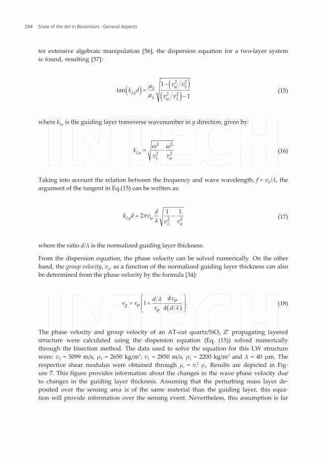
The phase velocity and group velocity of an AT-cut quartz/SiO2 Z’ propagating layeredstructure were calculated using the dispersion equation (Eq. (15)) solved numericallythrough the bisection method. The data used to solve the equation for this LW structurewere: vS = 5099 m/s, ρS = 2650 kg/m3, vL = 2850 m/s, ρL = 2200 kg/m3 and λ = 40 μm. Therespective shear modulus were obtained through μi = vi

2 ρi. Results are depicted in Fig‐ure 7. This figure provides information about the changes in the wave phase velocity dueto changes in the guiding layer thickness. Assuming that the perturbing mass layer de‐posited over the sensing area is of the same material than the guiding layer, this equa‐tion will provide information over the sensing event. Nevertheless, this assumption is far


from the biosensors reality, where the consideration of a five–layer model is required (seeFigure 1b).

Running Title 15

2 2

2 2

1tan

1

SSLy

L L

v vk d

v v

(0.15) 1

where kLy is the guiding layer transverse wavenumber in y direction, given by: 2

2 2

2 2LyL

kv v

(0.16) 3

Taking into account the relation between the frequency and wave wavelength, f = vφ/λ, the argument 4 of the tangent in Eq.(0.15) can be written as: 5

2 2

1 12Ly

L

dk d v

v v

(0.17) 6

where the ratio d/λ is the normalized guiding layer thickness. 7

From the dispersion equation, the phase velocity can be solved numerically. On the other hand, the 8 group velocity, vg, as a function of the normalized guiding layer thickness can also be determined 9 from the phase velocity by the formula [34]: 10

d

1dg

vdv v

v d

(0.18) 11

The phase velocity and group velocity of an AT-cut quartz/SiO2 Z’ propagating layered structure 12 were calculated using the dispersion equation (Eq. (0.15)) solved numerically through the bisection 13 method. The data used to solve the equation for this LW structure were: vS = 5099 m/s, 14 ρS = 2650 kg/m3, vL = 2850 m/s, ρL = 2200 kg/m3 and λ = 40 μm. The respective shear modulus were 15 obtained through μi = vi

2 ρi. Results are depicted in Figure 7. This figure provides information about 16 the changes in the wave phase velocity due to changes in the guiding layer thickness. Assuming that 17 the perturbing mass layer deposited over the sensing area is of the same material than the guiding 18 layer, this equation will provide information over the sensing event. Nevertheless, this assumption is 19 far from the biosensors reality, where the consideration of a five–layer model is required (see Figure 20 1b). 21

d/λ

Vel

ocit

y (m

/s)

0 0.2 0.4 0.6 0.8 12500

3000

3500

4000

4500

5000

5500

Figure 7. a) AT-cut Z’ propagating quartz/SiO2 phase velocity (continuous line) and group velocity (dashed line) for λ = 40 μm.

Figure 7. a) AT-cut Z’ propagating quartz/SiO2 phase velocity (continuous line) and group velocity (dashed line) for λ =40 μm.

Mc Hale et al. developed the dispersion equation of three and four-layer systems neglectingpiezoelectricity of the substrate [33]. When the substrate piezoelectricity is not considered,the dispersion equation is simplified. This can be the case of quartz substrates, which piezo‐electricity is low. However, as the piezoelectricity of a substrate increases (like in the case ofLT and LN), neglecting piezoelectricity, or assuming it is accounted for a stiffening effect inthe phase velocity, may be less valid [58]. Liu et al. provided a theoretical model for analyz‐ing the LW in a multilayered structure over a piezoelectric substrate [58]. Nevertheless, inour opinion, for those applications with a high number of layers, as in the case of biosensors,the use of the TLM is more convenient, since it is a very structured and intuitive modelwhere the addition of an extra layer does not make the procedure more complex. From theprogramming point of view, this is an enormous advantage.

The phase velocity provided by the dispersion equation can be used to determine the opti‐mal guiding layer thickness, which provides a maximum sensitivity. This issue will be ad‐dressed in Section 5.

4.3. LW sensor 3D FEM simulations

The models mentioned before, applied simplifying assumptions like considering the devicesubstrate as isotropic and neglecting the substrate piezoelectricity. This makes the modelsfar from the LW device reality. For a more accurate calculation of piezoelectric devices oper‐ating in the sonic and ultrasonic range, numerical methods such as finite element method(FEM) or boundary element methods (BEM) are the preferred choices [59]. The combinationof the FEM and BEM (FEM/BEM) has been used by many authors for the simulation of SAW


295

devices [60]. Periodic Green’s functions [61] are the basis of this model. However, theFEM/BEM only applies to infinite periodic IDTs and it is a 2 dimensional (2D) analysis.Thus, this method is only an approximation of a real finite SAW device.

Simulations of piezoelectric media require the complete set of fundamental equations relat‐ing mechanical and electrical phenomena in 3 dimensions (3D). The 3D-FEM can handlethese types of differential equations. The FEM formulation for piezoelectric SAW devices iswell explained in [59]. In general, the procedure for simulating LW devices using the 3D-FEM is the following: 1) the 3D model of the device is build using a computer-aided design(CAD) software; 2) the 3D model is imported to a commercial finite element software,which allows piezoelectric analysis; 3) the material properties of the involved materials areintroduced in the software; 4) the convenient piezoelectric finite element is selected; 5) themodel is meshed with the selected finite element; and 6) the simulation is run in the soft‐ware. As result the software obtains the particle displacements and voltage at every nodeof the model.

Although 3D-FEM simulations are extremely useful tools for studying LW device electro-acoustic interactions, LW simulations in real size are still a challenge. Delay lines in practiceare of many wavelengths and simulate them would require having too many finite ele‐ments. Thus, further efforts are required in order to achieve simulations able to reproducereal cases, which do not consume excessive computational resources. Nevertheless, someauthors have simulated scaled LW sensors using this method [62-65].

5. Sensitivity and limit of detection

A key parameter when designing a LW biosensor is the device sensitivity [13]. In generalterms, the sensitivity is defined as the derivative of the response (R) with respect to thephysical quantity to be measured (M):

0limM

R dRSM dMD ®

D= =

D(19)

It is possible to have different units of sensitivity depending on the used sensor response.E.g. for frequency output sensors, frequency (R = f), relative frequency (R = f / f0), frequencyshift (R = f - f0) and relative frequency shift (R = ( f - f0 )/ f0) can be found, being f0 the nonperturbed starting frequency. Hence, four different possibilities of sensitivity formats arepossible, and therefore it is extremely important to mention which case is been used in eachapplication.

The sensitivity of LW sensors gives the correlation between measured electric signals deliv‐ered by the sensor and a perturbing event which takes place on the sensing area of the sen‐sor. A high sensitivity relates a strong signal variation with a small perturbation [32].Depending on the used electronic configuration, the electrical signal measured in LW devi‐


ces can be: operation frequency, amplitude (or Insertion Loss), and phase. From this signal,and using the theoretical models, the phase velocity and group velocity can be obtained (seeSections 4.1 and 4.2).

When the sensor response R is the phase velocity, and the perturbing event which takesplace on the sensing area is a variation of the surface mass density of the coating σ (σ=h ρC),the velocity mass sensitivity Sv

σ of a LW device at a constant frequency is given by [32,66]:

0

1v

f

vS

vj

sj s

¶=

¶ (20)

where vφ0 is the unperturbed phase velocity and vφ is the phase velocity after a surface masschange.

Hence, Svσ has units of m2/kg. In Eq. (20) partial derivatives have been considered as the

phase velocity depends on several variables. The surface mass sensitivity reported for LWdevices in literature are between 150-500 cm2/g [45,67].

In sensor applications the phase velocity shift must be obtained from the experimental val‐ues of phase or frequency shifts. For the closed loop configuration, where the experimental‐ly measured quantity is the frequency, the frequency mass sensitivity Sf

σ is defined as:

0

1f dfSf ds s

= (21)

Jakoby and Vellekoop [66] noticed that the sensitivity measured by frequency changes in anoscillator (Eq. (21)) differs from the estimated velocity mass sensitivity (Eq. (20)) by a factorvg/vφ, since Love modes are dispersive. Thus, a typical 10% difference can be noted betweenSf

σ and Svσ.

For the open loop configuration, where the experimentally measured quantity is the phase,the phase sensitivity (also called gravimetric sensitivity) Sφ

σ in absence of interference is de‐fined as:

1 v

Lz

dS Sk D d

js s

js

= = (22)

where D is the distance between input and output IDT (see Figure 3) and kLz is the wave‐number of the Love mode, therefore kLzD is the unperturbed phase φ0.

The theoretical mass sensitivity of LW devices, derived from the perturbation theory[55],can be determined from the phase velocity according to [57]:


297

12sin( )cos( ) cos ( )1 1 Ly Ly Lyv S

L Ly L Sy

k d k d k dS

d k d k dsr

r r

-æ ö- ç ÷= + +ç ÷è ø

(23)

where kLy is the wavenumber in the guiding layer (Eq. (16)) and kSy is the wavenumber in thesubstrate (Eq. (24)). The minus sing in Eq. (23) indicates that the phase velocity of the pertur‐bed event due to an increment in the surface mass density is less than the unperturbedphase velocity (Δvφ = vφ- vφ0).

2 2

2 2SyS

kv vj

w w= - (24)

The phase velocity can be obtained with the dispersion equation (see Figure 7) or transmis‐sion line model. Once the phase velocity is known, the mass sensitivity curve can be ob‐tained using Eq. (23). In Figure 8, the dependence of the sensitivity with the guiding layerthickness for an AT-cut quartz/SiO2 Z’ propagating structure is depicted. A maximum masssensitivity Sv

σ of -39.44 m2/kg is observed at d/λ of 0.171 which corresponds to a d = 6.84 μm.The phase velocity at d/λ = 0.171 is vφ = 4140 m/s (see Figure 7) which leads to a synchronousfrequency fs = vφ/λ = 103.5 MHz.

Figure 8. a) AT-cut quartz Z’ propagating /SiO2 mass sensitivity considering λ = 40 μm.

Thus, as mentioned previously, for very small thicknesses compared to the wavelength, theacoustic field is not confined to the surface and deeply penetrates into the piezoelectric sub‐strate, resulting in low mass sensitivity [68]. If the thickness is increased the sensitivity rises,


as the acoustic energy is more efficiently trapped in the guiding layer. However, an exces‐sive increase in the guiding layer thickness leads to a reduction of wave energy density andthe mass sensitivity decreases [69]. Therefore, there is an optimal guiding layer thickness atwhich a maximum mass sensitivity is achieved for a specific wavelength.

In those applications where a coating layer in contact with a liquid is deposited over thesensing area, such is the case for biosensors, both changes in the surface mass density Δσand in the mass viscosity Δ(ρCηC)1/2 of the coating occur, due to the biochemical interactionbetween the coating and the liquid medium. In this case, the sensitivity can be modeled bythe four components matrix shown in Eq.(25) [15]. These components relate shifts in surfacemass density and in mass viscosity to the measured electrical signals: phase shift φ and Inser‐tion Loss (IL). The matrix components relate shifts of surface density Δσ and mass viscosityΔ(ρη)1/2 to shifts of electrical phase Δφ and signal attenuation ΔIL. Notice that Sφ,σ is not thesame than Sφ

σ in Eq.(22).

, ,

, ,

C C

C CC CIL IL

S S

IL S S

j s j r h

s r h

sjr h

æ ö é ùDé ùD ç ÷= ê úê ú ç ÷D Dê úë û ç ÷ ë ûè ø

(25)

Generally, the high sensitivity of microacoustic sensors is closely related to the fact that theyshow a high temperature stability (low TCF) and a large signal-to-noise ratio, which, in turnyields low detection limits and a high resolution of the sensor [13]. The limit of detection(LOD) is a very important characteristic of acoustic biosensors, since it gives the minimumsurface mass that can be detected by the device. It can be directly derived from the ratio be‐tween the noise in the measured electrical signal Nf and the sensitivity of the device. For in‐stance, in a closed loop configuration, this noise Nf is the RMS value of the frequencymeasured over a given period of time in stable and constant conditions [32]. It is usually rec‐ommended to measure a signal variation higher than 3 times the noise level in order to con‐clude from an effective variation [70]. From this recommendation, it comes out that the LODis given by [32,71]:

min

3LOD f

f

N

S fs

s×

= =×

(26)

where f is the operation frequency.

The LOD is improved by minimizing the influence of temperature on the sensor re‐sponse [13]. The stability with respect to temperature can be achieved by implementingtemperature control in the biosensor system and choosing materials of low TCF, as seenin Section 2.1.


299

6. LW packaging and flow cells

Flow cells are usually constructed with an inlet at one side, an outlet at the other, and thechannels facing the sensor (see Figure 9). In most cases, a rubber seal is used for sealing, andin LW flow-cells additional absorbers made with rubber materials at the ends of the IDTsare recommended to improve the signal response (see Figure 9b). Factors such as the flowcell design, flow patterns and flow-through system influence the binding efficiency and thecourse of binding kinetics, resulting in possible variations of the true results [72].

The permittivity and the dielectric losses of the liquid medium, necessary in LW biosensorsapplications, influence the propagation of Love modes, since this medium acts as an addi‐tional layer. When the liquid medium is deposited over the device surface, the presence ofthis medium over the IDTs modifies the electrodes transfer function [73]. Permittivity anddielectric losses of the liquid lead to a corresponding change of the IDT input admittance,which influences the amplitude of the signal. A flow–through cell is crucial to eliminate thiselectric influence of the liquid. Such flow-cell isolates the IDTs from the liquid, confining theliquid in the region between the IDTs (sensing area). LW device packaging or flow-cells gen‐erally use walls to accomplish this purpose. These walls, when pressed onto the device sur‐face, disturb the acoustic wave, resulting in an increase in overall loss and distortion of thesensor response. Walls must be designed to minimize the contact area in the acoustic path inorder to obtain the minimum acoustic attenuation (see Figure 9c). It is known that the acous‐tic wave is significantly affected when increasing the walls width [27] and that materialsused for these walls play an important role. Hence, great care must be taken to ensure thatthe designed LW flow cells do not greatly perturb the acoustic signal. Recently, some re‐searchers have explored different possibilities to achieve the packaging of LW sensors forfluidic applications [27,74] and other authors have being exploring different LW flow-cellapproaches [53,75,76].

PDMS absorbers

PDMS seal

b)

Inlet

Outlet

LW sensor

a)

Sensing area PDMS seal

c) Inlet

Outlet

Transparent PMMA Aluminum

Figure 9. A developed LW flow cell for immunosensors application designed and fabricated by the authors of thischapter [53]. a) Overview of the flow cell b) Microscope view through the PMMA of the LW sensor and flow cell ele‐ments. c) PDMS square seal with pick end to minimize the contact area.


Further improvements for LW biosensors flow cells can be achieved, since it is an entirelynew field and the development trends moves towards smaller flow cells which allows theuse of less analyte. For instance, investigation on the materials used for creating flow cells,packaging, and flow patterns in microfluidic channels [72] would enhance LW performanceand move them faster to the lab-on-a-chip arena.

7. LW biosensors state-of-the-art

The first approaches employing LW for biochemical sensing were reported in 1992 by Ko‐vacs et al. [77] and by Gizeli et al. [78], who first demonstrated the use of such devices asmass sensing biosensors in liquids. However, it was not until 1997 that LW acoustic deviceswere used to detect real-time antigen-antibody interactions in liquid media [46].

In 1999, a contactless LW device was built in order to protect electrodes from the conductiveand chemically aggressive liquids used in biosensing [79]. The advantage of this technique isthat no bonding wires are required.

In 2000, a dual channel LW device was used as a biosensor to simultaneously detect Legion‐ella and E. coli by Howe and Harding [80]. In this approach a novel protocol for coating bac‐teria on the sensor surface prior to addition of the antibody was introduced. Quantitativeresults were obtained for both species down to 106 cells/mL, within 3 h.

In 2003, a LW immunosensor was designed as a model for virus or bacteria detection in liq‐uids (drinking or bathing water, food, etc.) by Tamarin et al. [47]. They grafted a monoclonalantibody (AM13 MAb) against M13 bacteriophage on the device surface (SiO2) and sensedthe M13 bacteriophage/AM13 immunoreaction. The authors suggested the potentialities ofsuch acoustic biosensors for biological detection. The same year, it was shown that masssensitivity of LW devices with ZnO layer was larger than that of sensors with SiO2 guidinglayers [48]. The authors of this work monitored adsorption of rat immunoglobulin G, obtain‐ing mass sensitivities as high as 950 cm2/g. They pointed out that such a device was a prom‐ising candidate for immunosensing applications.

An aptamer-based LW sensor which allowed the detection of small molecules was devel‐oped by Schlensog et al. in 2004 [81]. This biosensor offers an advantage over immunosen‐sors, since it does not require the production of antibodies against toxic substances. A LWbiosensor for the detection of pathogenic spores at or below inhalational infectious levelswas reported by Branch et al. in 2004 [20]. A monoclonal antibody with a high degree of se‐lectivity for anthrax spores was used to capture the non-pathogenic simulant Bacillus thurin‐giensis B8 spores in aqueous conditions. The authors stated that acoustic LW biosensors willhave widespread application for whole-cell pathogen detection.

Moll et al. developed an innovative method for the detection of E. coli employing an LW de‐vice in 2007 [49]; it consisted of grafting goat anti-mouse antibodies (GAM) onto the sensorsurface and introducing E. coli bacteria mixed with anti-E. coli MAb in a second step. Thesensor response time was shorter when working at 37°C, providing results in less than 1


301

hour with a detection threshold of 106 bacteria/mL. More recently, the same group describeda multipurpose LW immunosensor for the detection of bacteria, virus and proteins [82].They successfully detected bacteriophages and proteins down to 4 ng/mm2 and E.coli bacte‐ria up to 5.0 × 105 cells in a 500 μL chamber, with good specificity and reproducibility. Theauthors stated that whole bacteria can be detected in less than one hour.

Andrä et al. used a LW sensor to investigate the mode of action and the lipid specificity ofhuman antimicrobial peptides [83]. They analyzed the interaction of those peptides withmodel membranes. These membranes, when attached to the sensor surface, mimic the cyto‐plasmic and the outer bacterial membrane. A LW immunosensor was used in 2008 by Bisoffiet al. [84] to detect Coxsackie virus B4 and Sin Nombre Virus (SNV), a member of the hanta‐virus family. They described a robust biosensor that combines the sensitivity of SAW at afrequency of 325 MHz with the specificity provided by monoclonal and recombinant anti‐bodies for the detection of viral agents. Rapid detection (within seconds) for increasing virusconcentrations was reported. The biosensor was able to detect SNV at doses lower than theload of virus typically found in a human patient suffering from hantavirus cardiopulmonarysyndrome.

In 2009, it was shown the possibility to graft streptavidin-gold molecules onto a LW sensorsurface in a controlled way and was demonstrated the capability of the sensor to detectnano-particles in aqueous media by Fissi et al. [85]. In 2010, a complementary metal–oxidesemiconductor CMOS-LW biosensor for breast cancer biomarker detection was presented byTigli et al. [36]. This biosensor was fabricated using CMOS technology and used gold asguiding layer and as interface material between the biological sensing medium and thetransducer.

LW devices were used as sensors for okadaic acid immono-detection through immobilizedspecific antibodies by Fournel et al. [76]. They obtained three times higher frequency shiftswith the okadaic acid than with an irrelevant peptide control line. A LW based bacterial bio‐sensor for the detection of heavy metal in liquid media was reported in 2011 by Gammoudiet al. [86]. Whole bacteria (E. coli) were fixed as bioreceptors onto the acoustic path of thesensor coated with a polyelectrolyte multilayer using a layer by layer electrostatic self-as‐sembly procedure. Changes of bacteria viscoelastic equivalent parameters in presence oftoxic heavy metals were monitorized.

A LW-based wireless biosensor for the simultaneous detection of Anti- Dinitrophenyl-KLH(anti-DNP) immunoglobulin G (IgG) was presented by Song et al. in 2011 [87]. They usedpoly(methyl-methacrylate) (PMMA) guiding layer and two sensitive films (Cr/Au). A LWsensor whose phase shifts as a function of the immobilized antibody quantity, combinedwith an active acoustic mixing device, was proposed by Kardous et al. [88] in 2011. They as‐sessed that mixing at the droplet level increases antibodies transfer to a sensing area surfaceand increases the reaction kinetics by removing the dependency with the protein diffusioncoefficient in a liquid, while inducing minimum disturbance to the sensing capability of theLove mode. LW sensors have been also used to study the properties of protein layers [40],DNA [89,90] and detect the adsorption and desorption of a lipid layer [91].


Currently, the only commercial LW biosensor system available in the market is commercial‐ized by the German company SAW instruments GmbH. The sensor system can achieve a limitof detection (LOF) of 0.05 ng/cm2 with a sample volume of 40-80 μL. Senseor company (Mou‐gins, France) has a commercially available microbalance development kit (SAW-MDK1)which consists of a two-channel LW delay lines.

8. Trends and future challenges of LW sensors

LW biosensors have not been very well recognized by the scientific community [72] nor bythe market yet. This might be due to the technological hindrances found for applying thisdevice as biosensor, since it is sensitive to changes in the viscoelastic properties of the coat‐ing, which complicates the results interpretation. Reports about applications where mass al‐terations are separated from viscoelastic effects can enhance the acceptance of LW sensors[72]. Hence, it is necessary to investigate different alternatives for carrying out the procedureof parameters extraction with LW sensors. Nowadays, the trend is the placement of multi‐ple, small, versatile sensors into a network configured for a specific location [10]. LW devi‐ces will move into the lab-on-a chip arena during the next years. Nevertheless, LW devicesstill have some hurdles to clear. LW biosensors packaging needs further development andcost reduction. In addition, much research and efforts are still required addressing the fluid‐ic technology issue. Integration and automation with electronics and flow cells reduce costsof the system and increase the throughput. For a better performance of LW sensors, the com‐bination with other detection methods such as optical [32] or chromatographic [92] are beingconsidered.

Mathematical modeling and simulations of these devices are also essential for the develop‐ment of new sensors, especially with respect to the study of new materials and wave propa‐gation [72]. Numerical calculations and FEM analysis of LW sensors could help for furtherunderstanding of these devices.

Author details

María Isabel Rocha Gaso1,2, Yolanda Jiménez1, Laurent A. Francis2 and Antonio Arnau1

*Address all correspondence to: [email protected]

1 Wave Phenomena Group, Department of Electroic Engineering, Universitat Politècnica deValència, Spain

2 Sensors, Microsystems and Actuators Laboratory of Louvain (SMALL), ICTEAM Institute,Université Catholique de Louvain, Belgium


303

References

[1] March C, Manclús JJ, Jiménez Y, Arnau A, Montoya A. A piezoelectric immunosen‐sor for the determination of pesticide residues and metabolites in fruit juices. Talanta2009;78(3) 827-833.

[2] Lucklum R, Soares D, Kanazawa K. Models for resonant sensors. In: Arnau A. (ed.)Piezoelectric transducers and applications. Springer; 2008. p63-96.

[3] Janshoff A, Galla HJ, Steinem C. Piezoelectric mass-sensing devices as biosensors- analternative to optical biosensors? Angew. Chem. Int. Ed. 2000;39 4005-4032.

[4] Andle JC and Vetelino JF. Acoustic wave biosensors. Sens. Actuators, A 1994;44167-176.

[5] Länge K, Rapp BE, Rapp M. Surface acoustic wave biosensors: a review. Anal. Bioa‐nal. Chem. 2008;391(5) 1509-1519.

[6] Smith JP and Hinson-Smith V. Commercial SAW sensors move beyond military andsecurity applications. Anal. Chem. 2006; 3505-3507.

[7] Weber J, Link M, Primig R, Pitzer D, Wersing W, Schreiter M. Investigation of thescaling rules determining the performance of film bulk acoustic resonators operatingas mass sensors. IEEE Trans. Ultrason. Ferroelectr. Freq. Cont. 2007;54(2) 405-412.

[8] Oliner AA. Microwave network methods for guided elastic waves. IEEE Trans. Mi‐crowave Theory Tech. 1969;17(11) 812-826.

[9] Voinova MV. On Mass Loading and Dissipation Measured with Acoustic Wave Sen‐sors: A Review. Journal of Sensors 2009; 1-13.

[10] Rocha-Gaso M-I, March-Iborra C, Montoya-Baides A, Arnau-Vives A. Surface gener‐ated acoustic wave biosensors for the detection of pathogens: a review. Sensors2009;9 5740-5769.

[11] Ballato A. Piezoelectricity: old effect, new thrusts. IEEE Trans. Ultrason. Ferroelectr.Freq. Cont. 1995;42(5) 916-926.

[12] Francis LA. Investigation of Love waves sensors. Optimisation for biosensing appli‐cations. Master Thesis. Université Catholique de Louvain; 2001.

[13] Jakoby B, Bastemeijer J, Vellekoop MJ. Temperature-compensated Love-wave sen‐sors on quartz substrates. Sens. Actuators, A 2000;82((1-3)) 83-88.

[14] Herrmann F and Büttgenbach S. Temperature-compensated Shear Horizontal surfaceacoustic wave in layered quartz/SiO2- structures. Physica status solidi 1998;170 R3-R4.

[15] Du J and Harding GL. A multilayer structure for Love-mode acoustic sensors. Sens.Actuators, A 1998;65 152-159.


[16] Tamarin O, Déjous C, Rebiere D, Pistré J, Comeau S, Moynet D, Bezian J. Study ofacoustic Love wave devices for real time bacteriophage detection. Sens. Actuators, B2003;91 275-284.

[17] Herrmann F, Weihnacht M, Buttgenbach S. Properties of sensors based on shear-hor‐izontal surface acoustic waves in LiTaO3/SiO2 and quartz/SiO2 structures. IEEETrans. Ultrason. Ferroelectr. Freq. Cont. Jan.2001;48(1) 268-273.

[18] Kalantar-Zadeh K, Powell DA, Sadek AZ, Wlodarski W, Yang QB, Li YX. Compari‐son of ZnO/64° LiNbO3 and ZnO/36° LiTaO3 surface acoustic wave devices for sens‐ing applications. Sens. Lett. 2006;4(2) 135-138.

[19] Hickernell FS, Knuth HD, Dablemont RC, Hickernell TS. The surface acoustic wavepropagation characteristics of 64° YX LiNbO3 and 36° YX LiTaO3 substrates withthin-film SiO2. In: proceedings of the IEEE Ultrason.Symp., Seattle, USA. 1995.

[20] Branch DW and Brozik SM. Low-level detection of a Bacillus anthracis simulant us‐ing Love-wave biosensors on 36° YX LiTaO3. Biosens. Bioelectron. 2004;19 849-859.

[21] Branch DW and Thayne LE. 4D- 4 Love wave acoustic array biosensor platform forautonomous detection. In: proceedings of the IEEE Ultrason.Symp., 2007.

[22] Gizeli E, Bender F, Rasmusson A, Saha K, Josse F, Cernosek R. Sensitivity of theacoustic waveguide biosensor to protein binding as a funcion of the waveguideproperties. Biosens. Bioelectron. 2003;18 1399-1406.

[23] Powell DA, Kalantar-Zadeh K, Wlodarski W. Numerical calculation of SAW sensitiv‐ity: application to ZnO/LiTaO3 transducers. Sens. Actuators, A 2004;115 456-461.

[24] White RM and Voltmer FW. Direct piezoelectric coupling to surface elastic waves.Appl. Phys. Lett. 1965;7(12) 314-316.

[25] Nieuwenhuizen MS and Venema A. Surface acoustic wave chemical sensors. Sens.Mater. 1989;5 261-300.

[26] Morgan DP. Surface-Wave Devices for Signal Processing. Elsevier Science PublishersB.V.; 1991.

[27] El Fissi L. Détection et mesure de nanoparticules pour les applications de capteurs enmilieu liquide. PhD Thesis. Université de Franche-Comté; 2009.

[28] Hashimoto K-Y. Surface Acoustic Wave Devices in Telecommunications. Springer-Verlag; 2000.

[29] Campbell C. Surface acoustic wave devices and their signal processing applications.Academic Press; 1989.

[30] Mazein P. Étude de dispositifs à ondes de Love par modélisation numérique de lapropagation d'ondes acoustiques. Application à l'optimisation de structures et à la


305

caractérisation de matériaux en vue de la réalisation de capteurs chimiques. PhDThesis. L'Université Bordeaux I; 2005.

[31] Du J, Harding GL, Ogilvy JA, Dencher PR, Lake M. A study of Love-wave acousticsensors. Sens. Actuators, A 1996;56 211-219.

[32] Francis LA. PhD Thesis. Thin film acoustic waveguides and resonators for gravimet‐ric sensing applications in liquid. PhD Thesis. Université Catholique de Louvain;2006.

[33] McHale G, Newton MI, Martin F. Theoretical mass,liquid,and polymer sensitivity ofacoustic wave sensorswith viscoelastic guiding layers. Appl. Phys. Lett. 2003;93(1)675-690.

[34] Barié N, Wessa T, Bruns M, Rapp M. Love waves in SiO2 layers on STW-resonatorsbased on LiTaO3. Talanta 2004;62 71-79.

[35] Gizeli E, Stevenson AC, Goddard NJ, Lowe CR. A novel Love-plate acoustic sensorutilizing polymer overlayers. IEEE Trans. Ultrason. Ferroelectr. Freq. Cont. 1992;39(5)657-659.

[36] Tigli O, Binova L, Berg P, Zaghloul M. Fabrication and characterization of a Surface-Acoustic-Wave biosensor in CMOS Technology for cancer biomarker detection. IEEETrans. Biomedical. Circuit. Systems. 2010;4(1) 62-73.

[37] Powell DA, Kalantar-Zadeh K, Ippolito S, Wlodarski W. 3E- 2 A layered SAW devicebased on ZnO/LiTaO3 for liquid media sensing applications, 1 ed 2002, pp. 493-496.

[38] Kalantar-Zadeh K, Trinchi A, Wlodarski W, Holland A. A novel Love-mode devicebased on a ZnO/ST-cut quartz crystal structure for sensing applications. Sens. Actua‐tors, A 2002;100 135-143.

[39] Matatagui D, Fontecha J, Fernández MJ, Aleixandre M, Gracia I, Cané C, HorrilloMC. Array of Love-wave sensors based on quartz/Novolac to detect CWA simulants.Talanta 2011;85 1442-1447.

[40] Saha K, Bender F, Rasmusson A, Gizeli E. Probing the viscoelasticity and mass of asurface-bound protein layer with an Acoustic Waveguide Device. Langmuir 2003;191304-1311.

[41] Herrmann F, Hahn D, Büttgenbach S. Separate determination of liquid density andviscosity with sagitally corrugated Love mode sensors. Sens. Actuators, A 1999;7899-107.

[42] Franssila S. Introduction to Microbabrication. Wiley; 2004.

[43] Gizeli E, Liley M, Lowe CL. Design considerations for the acoustic waveguide bio‐sensor. Smart Mater. Struct. 1997;6 700-706.


[44] El Fissi L, Friedt J-M, Ballandras S, Robert L, Chérioux F. Acoustic characterization ofthin polymer layers for Love mode surface acoustic waveguide. In: proceedings ofthe IEEE Int.Freq.Control Symp., 2008.

[45] Grate JW, Stephen JM, Richard MW. Acoustic wave microsensors. Anal. Chem.1993;65(21) 940A-848A.

[46] Harding GL, Du J, Dencher PR, Barnett D, Howe E. Love wave acoustic immunosen‐sor operation in liquid. Sens. Actuators, A 1997;61(1-3) 279-286.

[47] Tamarin O, Comeau S, Déjous C, Moynet D, Rebière D, Bezian J, Pistré J. Real timedevice for biosensing: design of a bacteriophage model using love acoustic wave. Bi‐osens. Bioelectron. 2003;18 755-763.

[48] Kalantar-Zadeh K, Wlodarski W, Chen YY, Fry BN, Galatsis K. Novel Love modesurface acoustic wave based immunosensors. Sens. Actuators, B 2003;91 143-147.

[49] Moll N, Pascal E, Dinh DH, Pillot JP, Bennetau B, Rebiere D, Moynet D, Mas Y, Mos‐salayi D, Pistre J, Dejous C. A Love wave immunosensor for whole E. coli bacteriadetection using an innovative two-step immobilisation approach. Biosens. Bioelec‐tron. Apr.2007;22(9-10) 2145-2150.

[50] Zimmermann B, Lucklum R, Hauptmann P, Rabe J, Büttgenbach S. Electrical charac‐terisation of high-frequency thickness-shear-mode resonators by impedance analysis.Sens. Actuators, B 2001;76 47-57.

[51] Montagut Y, Garcia JV, Jimenez Y, March C, Montoya A, Arnau A. Validation of aphase-mass characterization concept and interface for acoustic biosensors. Sensors(Basel) 2011;11(5) 4702-4720.

[52] Montagut YJ, Garcia JV, Jimenez Y, March C, Montoya A, Arnau A. Frequency-shiftvs phase-shift characterization of in-liquid quartz crystal microbalance applications.Rev. Sci. Instrum. 2011;82(6) 064702.

[53] Rocha-Gaso MI, March C, García J, El Fissi L, Francis LA, Jiménez Y, Montoya A, Ar‐nau A. User-friendly love wave flow cell for biosensors. In: proceedings of the Bio‐sensors 2012, Cancun, Mexico. 2012.

[54] Abdollahi A, Jiang A, Arabshahi SA. Evaluation on mass sensitivity of SAW sensorsfor different piezoelectric materials using finite-element analyisis. IEEE Trans. Ultra‐son. Ferroelectr. Freq. Contr. 2007;54(12) 2446-2455.

[55] Auld BA. Acoustic fields and waves in solids. Krieger; 1990.

[56] McHale G, Newton MI, Matin F. Layer guided shear horizontally polarized acousticplate modes. Appl. Phys. Lett. 2002;91 5735.

[57] Wang Z, Cheeke JDN, Jen CK. Sensitivity analysis for Love mode acoustic gravimet‐ric sensors. Appl. Phys. Lett. 1994;64(22) 2940-2942.


307

[58] Liu J and He S. Theoretical analysis on Love waves in layered structure with a piezo‐electric substrate and multiple elastic layers. J. Appl. Phys. 2010;107 073511.

[59] Sankaranarayanan SKRS, Bhethanabotla VR, Joseph B. Modeling of Surface AcousticWave Sensor Response. In: Ram MK, Bhethanabotla VR. (ed.) Sensors for Chemicaland Biological Applications. CRC Press; 2010. p97-134.

[60] Laude V, Reinhardt A, Ballandras S, Khelif A. Fast FEM/BEM computation of SAWharmonic admittance and slowness curves. In: proceedings of the IEEE Ultra‐son.Symp., 2004.

[61] Plessky VP and Thorvaldsson T. Rayleigh waves and leaky SAW's in periodic sys‐tems of electrodes: Periodic Green functions analysis. Electronics Letters 1992;281317-1319.

[62] Atashbar MZ, Bazuin BJ, Simpeh M, Krishnamurthy S. 3D FE simulation of H2 SAWgas sensor. Sens. Actuators, B 2005;111-112 213-218.

[63] Xu G. Finite element analysis of second order effects on the frequency response of aSAW device. In: proceedings of the IEEE Ultrason.Symp., 2000.

[64] Ippolito SJ, Kalantar-Zadeh K, Powell DA, Wlodarski W. A 3-dimensional finite ele‐ment approach for simulating acoustic wave propagation in layered SAW devices.In: proceedings of the IEEE Ultrason.Symp., 2003.

[65] Rocha-Gaso M-I, Fernandez-Díaz R, March-Iborra C, Arnau-Vives A. Mass sensitivi‐ty evaluation of a Love wave sensor using the 3D Finite Element Method. In: pro‐ceedings of the IEEE Int.Freq.Control Symp., 2010.

[66] Jakoby B and Vellekoop MJ. Properties of Love waves: applications in sensors. SmartMater. Struct. 1997;6 668-679.

[67] Ferrari V and Lucklum R. Overview of Acoustic-Wave Microsensors. In: Arnau A.(ed.) Piezoelectric transducers and applications. Springer; 2008. p39-59.

[68] Lee HJ, Namkoong K, Cho EC, Ko C, Park JC, Lee SS. Surface acoustic wave immu‐nosensor for real-time detection of hepatitis B surface antibodies in whole blood sam‐ples. Biosens. Bioelectron. June2009;24(10) 3120-3125.

[69] Kovacs G and Venema A. Theoretical comparison of sensitivities of acoustic shearwave modes for (bio) chemical sensing in liquids. Appl. Phys. Lett. 1992;61(6)639-641.

[70] MacDougall D, Amore FJ, Cox GV, Crosby DG, Estes FL, et.al. Guidelines for dataacquisition and data quality evaluation in environmental chemistry. Anal. Chem.1980;52(14) 2242-2249.

[71] Du J, Harding DR, Collings AF, Dencher PR. An experimental study of Love-waveacoustic sensors operating in liquids. Sens. Actuators, A 1997;60 54-61.


[72] Gronewold TM. Surface acoustic wave sensors in the bioanalytical field: recenttrends and challenges. Anal. Chim. Acta Nov.2007;603(2) 119-128.

[73] Jakoby B and Vellekoop MJ. Viscosity sensing using a Love-wave device. Sens. Ac‐tuators, A 1998;68 275-281.

[74] Francis LA, Friedt J-M, Bartic C, Campitelli A. A SU-8 liquid cell for surface acousticwave biosensors. In: proceedings of the SPIE - The International Society for OpticalEngineering, 2004.

[75] Tarbague H, Lachaud L, Vellutini L, Pillot JP, Bennetaur B, Moynet D, Rebière D.PDMS microfluidic chips combined to saw biosensors for ultra-fast biodetection ofantibodies and E. coli bacteria. In: proceedings of the Biosensors 2012, Cancun, Mexi‐co. 2012.

[76] Fournel F, Baco E, Mamani-Matsuda M, Degueil M, Bennetau B, Moynet D, Mossa‐layi D, Vellutini L, Pillot J-P, Dejous C, Rebiere D. Love wave biosensor for real-timedetection of okadaic acid as DSP phycotoxin. In: proceedings of the EurosensorsXXIV, Linz, Austria. 2010.

[77] Kovacs G, Lubking GW, Vellekoop MJ, Venema A. Love waves for (bio)chemicalsensing in liquids. In: proceedings of the IEEE Ultrason.Symp., Tucson, USA. 1992.

[78] Gizeli E, Goddard NJ, Lowe CR, Stevenson AC. A Love plate biosensor utilising apolymer layer. Sens. Actuators, B 1992;6 131-137.

[79] Freudenberg J, Schelle S, Beck K, von Schickfus M., Hunklinger S. A contactless sur‐face acoustic wave biosensor. Biosens. Bioelectron. 1999;14 423-425.

[80] Howe E and Harding G. A comparison of protocols for the optimisation of detectionof bacteria using a surface acoustic wave (SAW) biosensor. Biosens. Bioelectron.2000;15(11-12) 641-649.

[81] Schlensog MD, Thomas MA, Gronewold TM, Tewes M, Famulok M, Quandt E. ALove-wave biosensor using nucleic acids as ligands. Sens. Actuators, B 2004;101308-315.

[82] Moll N, Pascal E, Dinh DH, Lachaud J-L, Vellutini L, Pillot J-P, Rebière D, Moynet D,Pistré J, Mossalayi D, Mas Y, Bennetau B, Déjous C. Multipurpose Love acousticwave immunosensor for bacteria, virus or proteins detection. ITBM-RBM 2008;29155-161.

[83] Andrä J, Böhling A, Gronewold TMA, Schlecht U, Perpeet M, Gutsmann T. Surfaceacoustic wave biosensor as a tool to study the interactions of antimicrobial peptideswith phospholipid and lipopolysaccharide model membranes. Langmuir 2008;24(16)9148-9153.


309

[84] Bisoffi M, Hjelle B, Brown DC, Branch DW, Edwards TL, Brozik SM, Bondu-HawkinsVS, Larson RS. Detection of viral bioagents using a shear horizontal surface acousticwave biosensor. Biosens. Bioelectron. Apr.2008;23(9) 1397-1403.

[85] El Fissi L, Friedt J-M, Luzet V, Chérioux F, Martin G, Ballandras S. A Love-wave sen‐sor for direct detection of biofunctionalized nanoparticles. IEEE 2009; 861-865.

[86] Gammoudi I, Tarbague H, Lachaud JL, Destor S, Othmane A, Moyenet D, Kalfat R,Rebiere D, Dejous C. Love Wave Bacterial Biosensors and Microfluidic Network forDetection of Heavy Metal Toxicity. Sensor Letters 2011;9(2) 816-819.

[87] Song T, Song SY, Yoon HC, Lee K. Development of a wireless Love wave biosensorplatform for multi-functional detection. Japanese J. of Appl. Phys. 2011;50 1-6.

[88] Kardous F, El Fissi L, Friedt J-M, Bastien F, Boireau W, Yahiaoui R, Manceau JF, Bal‐landras S. Integrated active mixing and biosensing using low frequency vibrationmixer and Love-wave sensor for real time detection of antibody binding event. J.Appl. Phys. 2011;109 1-8.

[89] Tsortos A, Papadakis G, Mitsakakis K, Melzak KA, Gizeli E. Quantitative determina‐tion of size and shape of surface-bound DNA using an acoustic wave sensor. Bio‐phys. J. 2008;94 2706-2715.

[90] Papadakis G, Tsortos A, Gizeli E. Triple-helix DNA structural studies using a Lovewave acoustic biosensor. Biosens. Bioelectron. 2009;25 702-707.

[91] Gizeli E, Lowe CL, Liley M, Vogel H. Detection of supported lipid layers with theacoustic Love waveguidedevice: application to biosensors. Sens. Actuators, B 1996;34295-300.

[92] Marth M, Maier D, Stahl U, Rapp M, Wessa T, Honerkamp J. Optimization of surfaceacoustic wave sensor arrays and application to high performance liquid chromatog‐raphy. Sens. Actuators, B 1999;61 191-198.


589 ' # '6& *#5 & 7 - cdn.intechopen.comcdn.intechopen.com/pdfs-wm/43454.pdf ·...

Documents