6 front horn - quarter · pdf fileworksheet for front loaded horns, the calculated results are...

Section 6.0 : Design of a Front Loaded Exponential Horn By Martin J. King, 7/01/08

Copyright © 2008 by Martin J. King. All Rights Reserved.

of 26

Section 6.0 : Design of a Front Loaded Exponential Horn For a couple of years, a front loaded horn MathCad worksheet was available for downloading from my website. The worksheet was derived to simulate the front loaded horn geometry shown in Figure 6.1. The model solved the equivalent acoustic and electrical circuits as shown in Figures 6.2 and 6.3 respectively. A unit input of 1 watt into an assumed 8 ohm voice coil resistance, was applied as a constant voltage of 2.8284 volts RMS. There were minor updates to this worksheet over the years to extend the scope and correct a few minor bugs. At this point, a complete analysis of the equivalent circuits could be performed and the derivations would drag on for many pages. But this type of analysis, while providing some very useful sizing and limitation relationships, would probably not provide any intuitive feel for the workings of an exponential front loaded horn speaker. So instead of a rigorous mathematical derivation, which can be found in a number of other excellent technical references, the understanding gained in the preceding sections will be used to produce a set of simulations intended to characterize how a front loaded exponential horn works and what trade-offs can be made to optimize the final system performance. In all of the following simulations, it was assumed that the cross-sectional areas are circular. Square and rectangular cross-sectional areas will have to be examined later in a separate study. Probably the most important results presented so far are the resistive nature of the acoustic impedance of the horn and the potential for a large increase in the volume velocity ratio Ε above the lower cut-off frequency fc. This means that the front of the driver is radiating into a pure acoustic resistance that is a function only of the air density, the speed of sound, and the horn throat area.

Keeping this in mind, while looking again at Figure 6.1, we are left with a driver mounted in a closed box radiating into an acoustic resistance. Once the horn speaker system is recognized as being a driver in a closed box radiating into a pure acoustic resistance, the design problem can then be split into two separate sub-systems. Sizing the driver in a closed box as one sub-system and mating it to an appropriately sized exponential horn as a second sub-system will be the approach used in the following simulations. The two sub-systems are consistent if the same tuning frequency is used. A consistent design mates a driver in a closed box with an exponential horn geometry where both have the same tuning frequencies. This last statement is an important definition that will be assumed throughout the remainder of this document. The resulting motion of the driver’s cone, the driver’s volume velocity, is amplified by the horn to become an even greater volume velocity at the horn’s mouth. This result produces a dramatic increase in speaker efficiency compared to a closed or ported box. Looking back at Figures 5.2 through 5.5, there is no evidence of strong resonances in a correctly sized horn which would be seen as peaks in the magnitude response and rapid

= Zthroatρ cS0



of 26

phase shifts. All of this depends on the horn being sized to act as a horn and not as a resonant transmission line which was demonstrated in Figures 5.8 through 5.15.

Figure 6.1 : Front Loaded Horn Geometry

SL = SmouthS0 = Sthroat

Back ChamberFront Chamber

Lhorn

LFLB

S0B SDB SDF SLFHorn

where : Horn Geometry is defined by : S0 = Sthroat = throat area SL = Smouth = mouth area Lhorn = horn length Front Chamber Geometry is defined by : SDF = front chamber area at the driver end SLF = front chamber area at the throat end LF = front chamber length Back Chamber Geometry is defined by : SDB = back chamber area at the driver end S0B = back chamber area at the closed end LB = back chamber length



of 26

Figure 6.2 : Acoustic Equivalent Circuit for a Front Loaded Horn Speaker

Cad

pg

Ratd MadZab

Ud

Zal

Ud

p

where : pg = pressure source = (eg Bl) / (Sd Re) Rad = driver acoustic resistance = (Bl2 / Sd

2) [Qed / ((Rg + Re) Qmd)] Ratd = total acoustic resistance = Rad + (Bl)2 / [Sd

2 ((Rg + Re) + jω Lvc)] Cad = driver acoustic compliance = Vd / (ρair c2) Mad = driver acoustic mass

= (fd2 Cad)-1

Zab = back chamber acoustic impedance Zal = horn acoustic impedance (including front chamber) Ud = driver volume velocity = Sd ud ud = driver cone velocity then : UL = mouth air volume velocity = Ε Ud Ε = UL / Ud = volume velocity ratio

uL = mouth air velocity = ε ud

ε = uL / ud = velocity ratio



of 26

Figure 6.3 : Electrical Equivalent Circuit for a Front Loaded Horn Speaker

eg

Rg + Re Lvc

RedCmedLced Zeb Zeled

where : eg = voltage source = 2.8284 volt Rg+Re = electrical resistance of the amplifier, cables, and voice coil Lvc = voice coil inductance Lced = inductance due to the driver suspension compliance

= [Cad (Bl)2] / Sd2

Cmed = capacitance due to the driver mass

= (Mad Sd2) / (Bl)2

Red = resistance due to the driver suspension damping

= Re (Qmd / Qed)

Zel = horn equivalent electrical impedance (including front chamber) = (Bl)2 / (Sd

2 Zal) Zeb = back chamber equivalent electrical impedance = (Bl)2 / (Sd

2 Zal) ed = Bl ud



of 26

The Generic Driver : Before any simulations can be run, a generic driver needs to be defined that is easily adjustable to different combinations of Thiele / Small(8,9,10,11) parameters. The following driver parameters have been defined and are intended to represent a typical eight inch diameter full range driver such as those produced by Lowther, Fostex, or AER. All of the results that follow are really intended for full range driver applications but should also be applicable to larger woofer or mid-bass drivers. The generic full range driver is defined below based on key input properties and some derived properties. When looking at the relationships used to calculate the derived properties, please keep in mind that MathCad internally automatically converts frequency in Hertz to frequency in rad/sec. This property of MathCad leads to equations that may not look exactly like those familiar to the speaker designer. In equations containing a frequency term, a 2π multiplier may be missing or added depending on the desired units of the result.

Bl 12.9newton

amp=Bl

fd Re⋅ Mmd⋅

Qed

⎛⎜⎝

⎞

⎠

0.5

:=

dBSPL 96.0=SPL 112 10 log ηo( )⋅+:=

ηo 2.5%=ηo Vad 2 π⋅ c3⋅ Qed⋅ fd

3−⋅⎛

⎝⎞⎠

1−⋅:=

Vad 43.0liter=Vad Cmd ρ c2⋅ Sd

2⋅⎛

⎝⎞⎠⋅:=

Cmd 7.2 10 4−×

mnewton

=Cmd Mmd fd2

⋅⎛⎝

⎞⎠

1−:=

Qed 0.2=Qed1

Qtd

1Qmd

−⎛⎜⎝

⎞⎠

1−:=

Derived Thiele / Small Parameters

Sd 205 cm2⋅:=

Mmd 14 gm⋅:=Lvc 0 mH⋅:=

Qtd 0.2:=Re 8 ohm⋅:=

Qmd 4:=fd 50 Hz⋅:=

Driver Thiele / Small Parameters : Generic Driver Derivation

Now that a generic driver has been defined, baseline horn geometry can be formulated and a simulation run to calculate the on axis anechoic SPL response, the electrical impedance, and the impulse pressure response. Modifications can be made to



of 26

the generic driver, and the exponential horn geometry, to study the changes that occur in the calculated responses. Baseline Exponential Horn Design : The first simulation to be run, and the results presented, will be referred to as the baseline design. The lower cut-off frequency fc is specified as 150 Hz. A front chamber will not be included in the baseline horn geometry. The throat area is set equal to the driver’s Sd so that a length can be calculated. This style of horn system can be readily found on the Internet crossed over to bass enclosures yielding a complete full range speaker system. To start the design process, the area of the horn mouth is calculated using Equation (5.3). Smouth = (1 / π) x (c / (2 x fc))2 Smouth = (1 / π) x (342 m/sec / (2 x 150 Hz))2 Smouth = 0.414 m2 = 641.2 in2 Smouth = 20.2 x Sd Using Equation (5.2), the flare constant is calculated next. m = (4 π fc) / c m = (4 π 150 Hz) / 342 m/sec m = 5.512 m-1 And finally, the horn’s length is calculated using Equation (5.1) after setting the throat area equal to Sd. Lhorn = ln(Smouth / Sthroat) / m Lhorn = ln(20.2 / 1) / 5.512 m-1 Lhorn = 0.545 m = 21.5 in The horn sub-system geometry is now completely defined. To define the back chamber, a consistent approach is used by tuning the driver mounted in the back chamber to the same 150 Hz cut off frequency. Sizing of the horn geometry and the driver mounted in a sealed box are consistent since the same tuning frequencies are selected. Simple relationships for a closed box can be used to derive the back chamber volume and the resulting closed box alignment parameters.



of 26

The box tuning frequency is defined first. fb = 150 Hz Then the closed box Qtc parameter is calculated. Qtc = Qtd x (fb / fd) Qtc = 0.2 x (150 Hz / 50 Hz) Qtc = 0.6 And finally, the volume is calculated for the back chamber. Vb = Vad / ((Qtc / Qtd)2 - 1) Vb = 43 liter / ((0.6 / 0.2)2 - 1) Vb = 5.375 liter All of the geometry parameters have now been determined. The exact choice of cross-sectional area and length for the back chamber will have an impact on the SPL response when the frequency reaches a high enough value to generate standing waves inside the chamber. After substituting the dimensions and areas into a MathCad worksheet for front loaded horns, the calculated results are shown in Figure 6.4 and Figure 6.5. Figure 6.4 is the standard output format for all of the simulations that will be presented in this section. At the top of this figure, the driver parameters and horn geometry are restated. This is followed by plots of the anechoic on-axis SPL response at 1 m / 1 watt radiating into 2π space, the electrical impedance magnitude, and the pressure impulse response. In each plot, the horn system’s response is shown as a red solid curve. The same driver’s response when mounted in an infinite baffle is also shown as a blue dashed curve. This convention is used in all of the plots in this section. Several interesting results need to be highlighted in Figure 6.4. The first thing that jumps right out, when looking at the horn’s anechoic SPL plot (red solid curve) in Figure 6.4, is the deep null that appears in the on-axis response at approximately 5500 Hz. This is not an inherent property of the horn speaker; it is generated by the combination of a 1 m reference position and a large mouth radiating area. The path length differences between the simple sources used to simulate this large mouth area produce perfect cancellation of the summed SPL response at specific frequencies. As the reference position changes, the nulls move up or down in the frequency domain. This is demonstrated in Figure 6.6 for 0.5 m, 2.0 m, and 3.0 m reference positions. Also in the anechoic SPL response plot, the driver in an infinite baffle (blue dashed curve) is compared to the driver mounted in the horn system (red solid curve). Comparing the curves shows a 10 to 11 dB increase in output SPL for the horn system. The SPL response is fairly smooth, ignoring the nulls due to the 1 m listening position, and shows no sign of a resonant condition inside the horn.



of 26

This same conclusion can be reached after studying the impedance curve and the impulse response, there are no signs of extra peaks in the impedance curve or ringing in the impulse response that would be generated by resonances. Comparing the impedance curve for the infinite baffle (blue dashed curve) with the horn (red solid curve) shows that both exhibit single degree of freedom impedance magnitude curves. The impedance peak for the horn system is higher in frequency, compared to the infinite baffle curve, due to the closed box added to the back of the driver. Finally the displacement is plotted in Figure 6.5 for the infinite baffle (blue dashed curve) and the horn (red solid curve). Notice that the driver displacement, when mounted in the horn system, is significantly reduced just like in a closed box design. This is a very important result for eight inch full range drivers which typically have Xmax values of 1 mm. Not only is nonlinear distortion reduced but power handling is increased. With an appropriate bass enclosure, capable of generating a similar SPL, a full range high efficiency and high performance speaker system is achieved. The next few sections look at different variations to this baseline design and the impact this has on the calculated response. All plotted data will follow the format established in Figure 6.4. Again, please keep in mind that the solid red curves represent the response of the horn system and the dashed blue curves represent the response of the same driver mounted in an infinite baffle.



of 26

Figure 6.4 : Front Loaded Exponential Horn Response - Baseline Configuration

0 2 4 6 8 10 12 14 16 18 2020

10

0

10

20

30

40Impulse Pressure Response in Time Domain

Time (milliseconds)

psummedn

1000 Pa⋅

n dt⋅ 1000⋅

10 100 1 .1030

30

60

90

120

150Impedance Magnitude

Frequency (Hz)

Impe

danc

e (o

hms)

Zor

Z r

r dω⋅ Hz 1−⋅

10 100 1 .103 1 .10460

70

80

90

100

110

120On-Axis Anechoic SPL at 1 m / 1 watt

Frequency (Hz)

SPL

(dB

)

SPLor

SPLr

r dω⋅ Hz 1−⋅

Summary of Plotted Results

Lhorn 21.5in=Bl 12.93tesla m⋅=

Smouth 20.2Sd=Vad 43.0liter=

Sthroat 1.0Sd=Qtd 0.2=

fh 20000.0Hz=Re 8.0ohm=

fl 150.0Hz=fd 50.0Hz=

Horn SummaryDriver Summary



of 26

Figure 6.5 : Front Loaded Exponential Horn Response - Baseline Displacement Curve

10 100 1 .1030

1

2

3

4

5Driver Displacement

Frequency (Hz)

Def

lect

ion

(mm

)

xdr

mm

xr

mm

r dω⋅

Hz



of 26

Figure 6.6 : Front Loaded Exponential Horn Anechoic SPL Response as a Function of Reference Position

10 100 1 .103 1 .10460

70

80

90

100

110

120On-Axis Anechoic SPL at 0.5 m / 1 watt

Frequency (Hz)

SPL

(dB

)

SPLor

SPLr

r dω⋅ Hz 1−⋅

10 100 1 .103 1 .10460

70

80

90

100

110


Frequency (Hz)

SPL

(dB

)

SPLor

SPLr

r dω⋅ Hz 1−⋅

10 100 1 .103 1 .10460

70

80

90

100

110


Frequency (Hz)

SPL

(dB

)

SPLor

SPLr

r dω⋅ Hz 1−⋅



of 26

Changing the Throat Size : To study the impact of increasing or decreasing the throat area, three simulations were run and the results plotted. The baseline throat area of 1.0 x Sd was run along with throat areas of 0.5 x Sd and 2.0 x Sd. The plotted results are shown in Figures 6.7, 6.8, and 6.9 respectively and summarized below in Table 6.1.

Table 6.1 : Exponential Horn Throat Size Study Throat Area Mouth Area Length (in) SPL at 1 m / 1 w Resonance (Hz)

0.5 x Sd 20.2 x Sd 26.4 110 105 1.0 x Sd 20.2 x Sd 21.5 108 117 2.0 x Sd 20.2 x Sd 16.5 105 126

Comparing the plots in Figures 6.7, 6.8, and 6.9 it is obvious that the smaller the throat area the more efficient the exponential horn. The basic shape of the SPL response is the same for each horn but the maximum efficiency changes shifting the curve up or down in the plot relative to the baseline design. As the throat area decreases, the horn length increases. The increased horn length means that below the lower cut-off frequency fc, the air volume in the horn increases adding to the mass of the driver cone and voice coil. This change in the moving mass results in different resonant frequencies for the combined sub-systems. The last column in Table 6.1 lists the system’s resonant frequency as seen in the impedance magnitude plot. Also, as the efficiency changes, so does the pressure trace in the impulse response plot. Compared to the baseline simulations, the smaller throat produces a larger magnitude pulse with an additional time delay due to the longer horn geometry. The larger throat generates a smaller magnitude pulse with respect to the baseline simulation and a shorter time delay due to the shorter horn length. This is evident after reviewing the bottom plots in Figures 6.7, 6.8, and 6.9.



of 26

Figure 6.7 : Front Loaded Exponential Horn Response - Sthroat = 0.5 x Sd

0 2 4 6 8 10 12 14 16 18 2020

10

0

10

20

30


Time (milliseconds)

psummedn

1000 Pa⋅

n dt⋅ 1000⋅

10 100 1 .1030

30

60

90

120


Frequency (Hz)

Impe

danc

e (o

hms)

Zor

Z r

r dω⋅ Hz 1−⋅

10 100 1 .103 1 .10460

70

80

90

100

110


Frequency (Hz)

SPL

(dB

)

SPLor

SPLr

r dω⋅ Hz 1−⋅





fh 20000.0Hz=Re 8.0ohm=

fl 150.0Hz=fd 50.0Hz=




of 26

Figure 6.8 : Front Loaded Exponential Horn Response - Sthroat = 1.0 x Sd (Baseline)

0 2 4 6 8 10 12 14 16 18 2020

10

0

10

20

30


Time (milliseconds)

psummed n

1000 Pa⋅

n dt⋅ 1000⋅

10 100 1 .1030

30

60

90

120


Frequency (Hz)

Impe

danc

e (o

hms)

Zor

Z r

r dω⋅ Hz 1−⋅

10 100 1 .103 1 .10460

70

80

90

100

110


Frequency (Hz)

SPL

(dB

)

SPLor

SPLr

r dω⋅ Hz 1−⋅





fh 20000.0Hz=Re 8.0ohm=

fl 150.0Hz=fd 50.0Hz=




of 26

Figure 6.9 : Front Loaded Exponential Horn Response - Sthroat = 2.0 x Sd

0 2 4 6 8 10 12 14 16 18 2020

10

0

10

20

30


Time (milliseconds)

psummedn

1000 Pa⋅

n dt⋅ 1000⋅

10 100 1 .1030

30

60

90

120


Frequency (Hz)

Impe

danc

e (o

hms)

Zor

Z r

r dω⋅ Hz 1−⋅

10 100 1 .103 1 .10460

70

80

90

100

110


Frequency (Hz)

SPL

(dB

)

SPLor

SPLr

r dω⋅ Hz 1−⋅





fh 20000.0Hz=Re 8.0ohm=

fl 150.0Hz=fd 50.0Hz=




of 26

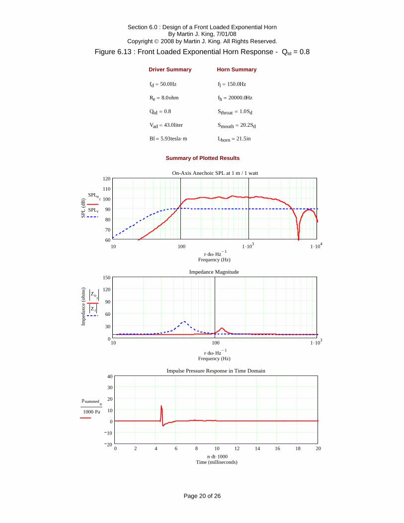
Changing the Driver’s Qtd Parameter : Traditionally, drivers with Qtd values between 0.15 and 0.25 are recommended for front loaded horns. These drivers usually have a very large powerful magnet resulting in a high Bl parameter and are extremely efficient with SPL’s approaching 98 – 100 dB at 1 m / 1 watt. It is typical to see strong comments on the Internet forums stating that a particular driver was designed strictly for horn loading. It is stated as a fact that cannot be questioned. This is a common theme when discussing some of the Lowther (PM2A, DX4, or EX4 model) or Fostex (FE-206E of FE-208 Sigma model) drivers. To investigate this observation, the baseline horn simulation will be rerun with the generic driver taking on Qtd values of 0.2, 0.4, 0.6, and 0.8. The horn and back chamber geometry will be held constant. Placing a higher Qtd driver in the same back chamber should lead to a closed box alignment that is severely under damped and far from an optimum flat sealed box alignment. Table 6.2 summarizes the test cases run and plotted in the following figures.

Table 6.2 : Driver Properties and Resulting Exponential Horn System Properties Driver Properties Qtd = 0.2 Qtd = 0.4 Qtd = 0.6 Qtd = 0.8 Bl (tesla-m) 12.92 8.90 7.06 5.93 Driver SPL (dB) 96.0 92.8 90.8 89.3 Horn Properties Qtc = 0.6 Qtc = 1.2 Qtc = 1.8 Qtc = 2.4 Horn SPL (dB) 108 104 102 101 Results for Qtd values of 0.2, 0.4, 0.6, and 0.8 are plotted in Figures 6.10, 6.11, 6.12, and 6.13 respectively. Reviewing the results in the table, it can be seen that as the Qtd increased the driver efficiency drops due to the decrease in the Bl parameter. After placing the higher Qtd drivers in the same back chamber, the combined Qtc becomes very large and typical of an under damped sealed box alignment. But looking at the SPL and impulse response plots, in the appropriate figures, there is no evidence of a ringing under damped low frequency response. In fact, other then the loss of horn system efficiency, the higher Qtd drivers extended lower in frequency and produced a smoother SPL response. The large mouth of the horn must be contributing a significant amount of damping to the entire horn system including the driver suspension. The loss of efficiency is a property of the driver; the boost provided by the horn remains constant at approximately 12 dB in all of the simulations.



of 26

Figure 6.10 : Front Loaded Exponential Horn Response - Qtd = 0.2

0 2 4 6 8 10 12 14 16 18 2020

10

0

10

20

30


Time (milliseconds)

psummed n

1000 Pa⋅

n dt⋅ 1000⋅

10 100 1 .1030

30

60

90

120


Frequency (Hz)

Impe

danc

e (o

hms)

Zor

Z r

r dω⋅ Hz 1−⋅

10 100 1 .103 1 .10460

70

80

90

100

110


Frequency (Hz)

SPL

(dB

)

SPLor

SPLr

r dω⋅ Hz 1−⋅





fh 20000.0Hz=Re 8.0ohm=

fl 150.0Hz=fd 50.0Hz=




of 26


0 2 4 6 8 10 12 14 16 18 2020

10

0

10

20

30


Time (milliseconds)

psummedn

1000 Pa⋅

n dt⋅ 1000⋅

10 100 1 .1030

30

60

90

120


Frequency (Hz)

Impe

danc

e (o

hms)

Zor

Z r

r dω⋅ Hz 1−⋅

10 100 1 .103 1 .10460

70

80

90

100

110


Frequency (Hz)

SPL

(dB

)

SPLor

SPLr

r dω⋅ Hz 1−⋅





fh 20000.0Hz=Re 8.0ohm=

fl 150.0Hz=fd 50.0Hz=




of 26

Compromised Exponential Horn Geometry Response : In Section 5.0, a series of plots were presented that depicted the evolution from straight transmission line geometry to exponential horn geometry. The results of this transition process are presented in Figures 5.8 through 5.15 and the individual steps defined in Table 5.2. The geometries that produce the impedances and volume velocity ratios plotted in Figure 5.12 and 5.13 were substituted for the baseline exponential horn geometry and the simulations rerun. The plotted output is shown in Figure 6.14 and 6.15 respectively. The results shown in Figure 6.14 and 6.15 are not “perfect” for the compromised horn geometry when compared to a consistently sized exponential horn system. The SPL responses show ripples in the lower frequency range and the impedance plot contains multiple peaks indicative of resonances in the horn itself. The impulse responses also exhibit ringing as the main pulse decays. And finally, the efficiency in both compromised horns is lower with respect to the baseline horn system shown in Figure 6.4. To determine if a particular enclosure is a consistently sized horn system, a review of the measured impedance magnitude would probably be a good indicator. If there is evidence of multiple impedance peaks then the enclosure is probably starting to act more like a transmission line or TQWT. A properly sized exponential horn, with consistent tuning frequencies for the back chamber and the horn geometry, will have only one predominant impedance peak.



of 26

Figure 6.14 : Compromised Front Loaded Exponential Horn Response

0 2 4 6 8 10 12 14 16 18 2020

10

0

10

20

30


Time (milliseconds)

psummedn

1000 Pa⋅

n dt⋅ 1000⋅

10 100 1 .1030

30

60

90

120


Frequency (Hz)

Impe

danc

e (o

hms)

Zor

Z r

r dω⋅ Hz 1−⋅

10 100 1 .103 1 .10460

70

80

90

100

110


Frequency (Hz)

SPL

(dB

)

SPLor

SPLr

r dω⋅ Hz 1−⋅





fh 20000.0Hz=Re 8.0ohm=

fl 150.0Hz=fd 50.0Hz=




of 26

Figure 6.15 : Compromised Front Loaded Exponential Horn Response

0 2 4 6 8 10 12 14 16 18 2020

10

0

10

20

30


Time (milliseconds)

psummedn

1000 Pa⋅

n dt⋅ 1000⋅

10 100 1 .1030

30

60

90

120


Frequency (Hz)

Impe

danc

e (o

hms)

Zor

Z r

r dω⋅ Hz 1−⋅

10 100 1 .103 1 .10460

70

80

90

100

110


Frequency (Hz)

SPL

(dB

)

SPLor

SPLr

r dω⋅ Hz 1−⋅





fh 20000.0Hz=Re 8.0ohm=

fl 150.0Hz=fd 50.0Hz=




of 26

Addition of a Front Chamber : The final simulation to be presented in this section will include a front chamber that rolls off the horn response at a higher cut-off frequency fh of 2500 Hz. The chamber volume V is calculated, in the same manner as demonstrated in Section 5, using Equation (5.4).

V = (342 m/sec x 0.010 m2) / (2 π 2500 Hz) x (1000 liters / m3) = 0.218 liters Placing this volume in series with the baseline horn geometry, and rerunning the MathCad simulation, produces the results plotted in Figure 6.16. Figure 6.16 exhibits a high frequency roll-off of the on axis anechoic SPL response as anticipated.



of 26

Figure 6.16 : Baseline Front Loaded Exponential Horn Response with a Front Chamber

0 2 4 6 8 10 12 14 16 18 2020

10

0

10

20

30


Time (milliseconds)

psummedn

1000 Pa⋅

n dt⋅ 1000⋅

10 100 1 .1030

30

60

90

120


Frequency (Hz)

Impe

danc

e (o

hms)

Zor

Z r

r dω⋅ Hz 1−⋅

10 100 1 .103 1 .10460

70

80

90

100

110


Frequency (Hz)

SPL

(dB

)

SPLor

SPLr

r dω⋅ Hz 1−⋅





fh 2500.0Hz=Re 8.0ohm=

fl 150.0Hz=fd 50.0Hz=




of 26

Summary : Rather then wade through many pages of mathematical derivations, this section used some simple sample problems to gain insight into how to design a front loaded exponential horn system. The key principle is to size the two sub-systems, the horn geometry and the driver in a closed back chamber, to have consistent tuning frequencies and then assemble these two sub-systems to form a front loaded exponential horn speaker. Sizing the exponential horn sub-system starts by sizing the mouth area for the lower cut-off frequency fc and then setting the throat area to determine the length and to provide the desired amount of SPL boost. A simulation program can be used to iterate the geometry parameters to quickly get an optimized result. Sizing the driver sub-system involves tuning a closed box design to the same lower cut-off frequency fc value as the horn sub-system. When sizing the front exponential horn sub-system, it is interesting to note that the driver’s size and Thiele / Small parameter do not enter into the calculations. The lower cut-off frequency fc determines the mouth cross-sectional area. The throat area and horn length are determined by the desired SPL boost above the lower cut-off frequency fc. Given two similar drivers that vary only in diameter, the same size horn mouth would result for the same low cut-off frequency fc. The same exponential front horn could be used for similar eight inch and six inch diameter drivers. With this basic understanding of the front loaded exponential horn, some advanced front loaded horn simulations will be investigated in articles to be presented independently at some later date.. The same approach characterizing the horn response using more advanced simulations, instead of a long mathematical derivation, will be used.

6 front horn - quarter · pdf fileworksheet for front loaded horns, the calculated results are...

Documents