6 relational markov networks - university of central...

6 Relational Markov Networks

Ben Taskar, Pieter Abbeel, Ming-Fai Wong, and Daphne Koller

One of the key challenges for statistical relational learning is the design of a repre-sentation language that allows flexible modeling of complex relational interactions.Many of the formalisms presented in this book are based on the directed graph-ical models (probabilistic relational models, probabilistic entity-relationship mod-els, Bayesian logic programs). In this chapter, we present a probabilistic modelingframework that builds on undirected graphical models (also known as Markov ran-dom fields or Markov networks). Undirected models address two limitations of theprevious approach. First, undirected models do not impose the acyclicity constraintthat hinders representation of many important relational dependencies in directedmodels. Second, undirected models are well suited for discriminative training, wherewe optimize the conditional likelihood of the labels given the features, which gen-erally improves classification accuracy. We show how to train these models effec-tively, and how to use approximate probabilistic inference over the learned modelfor collective classification and link prediction. We provide experimental results onhypertext and social network domains, showing that accuracy can be significantlyimproved by modeling relational dependencies.1

6.1 Introduction

We focus on supervised learning as a motivation for our framework. The vastmajority of work in statistical classification methods has focused on “flat” data– data consisting of identically structured entities, typically assumed to be i.i.d.However, many real-world data sets are innately relational: hyperlinked webpages,cross-citations in patents and scientific papers, social networks, medical records,and more. Such data consists of entities of different types, where each entity type is

1. This chapter is based on work in [21, 22].


characterized by a different set of attributes. Entities are related to each other viadifferent types of links, and the link structure is an important source of information.

Consider a collection of hypertext documents that we want to classify usingsome set of labels. Most naively, we can use a bag-of-words model, classifying eachwebpage solely using the words that appear on the page. However, hypertext has avery rich structure that this approach loses entirely. One document has hyperlinksto others, typically indicating that their topics are related. Each document alsohas internal structure, such as a partition into sections; hyperlinks that emanatefrom the same section of the document are even more likely to point to similardocuments. When classifying a collection of documents, these are important cuesthat can potentially help us achieve better classification accuracy. Therefore, ratherthan classifying each document separately, we want to provide a form of collectiveclassification, where we simultaneously decide on the class labels of all of the entitiestogether, and thereby can explicitly take advantage of the correlations between thelabels of related entities.

Another challenge arises from the task of predicting which entities are related towhich others and what are the types of these relationships. For example, in a dataset consisting of a set of hyperlinked university webpages, we might want to predictnot just which page belongs to a professor and which to a student, but also whichprofessor is which student’s advisor. In some cases, the existence of a relationshipwill be predicted by the presence of a hyperlink between the pages, and we will haveonly to decide whether the link reflects an advisor-advisee relationship. In othercases, we might have to infer the very existence of a link from indirect evidence,such as a large number of coauthored papers.

We propose the use of a joint probabilistic model for an entire collection ofrelated entities. Following the work of Lafferty et al. [13], we base our approach ondiscriminatively trained undirected graphical models, or Markov networks [17]. Weintroduce the framework of relational Markov networks (RMNs), which compactlydefines a Markov network over a relational data set. The graphical structure ofan RMN is based on the relational structure of the domain, and can easily modelcomplex patterns over related entities. For example, we can represent a patternwhere two linked documents are likely to have the same topic. We can also capturepatterns that involve groups of links: for example, consecutive links in a documenttend to refer to documents with the same label. As we show, the use of an undirectedgraphical model avoids the difficulties of defining a coherent generative model forgraph structures in directed models. It thereby allows us tremendous flexibility inrepresenting complex patterns.

Undirected models lend themselves well to discriminative training, where we op-timize the conditional likelihood of the labels given the features. Discriminativetraining, given sufficient data, generally provides significant improvements in clas-sification accuracy over generative training (see [23]). We provide an effective pa-rameter estimation algorithm for RMNs which uses conjugate gradient combinedwith approximate probabilistic inference (belief propagation [17, 14, 12]) for esti-mating the gradient. We also show how to use approximate probabilistic inference

6.2 Relational Classification and Link Prediction 177

over the learned model for collective classification and link prediction. We provideexperimental results on a webpage classification and social network task, showingsignificant gains in accuracy arising both from the modeling of relational depen-dencies and the use of discriminative training.

6.2 Relational Classification and Link Prediction

Consider hypertext as a simple example of a relational domain. A relational domainis defined by a schema, which describes entities, their attributes, and the relationsbetween them. In our domain, there are two entity types: Doc and Link. If a webpageis represented as a bag of words, Doc would have a set of Boolean attributesDoc.HasWordk indicating whether the word k occurs on the page. It would alsohave the label attribute Doc.Label, indicating the topic of the page, which takes ona set of categorical values. The Link entity type has two attributes: Link.From andLink.To, both of which refer to Doc entities.

In general, a schema specifies of a set of entity types E = {E1, . . . , En}. Eachtype E is associated with three sets of attributes: content attributes E.X (e.g.,Doc.HasWordk), label attributes E.Y (e.g., Doc.Label), and reference attributesE.R (e.g. Link.To). For simplicity, we restrict label and content attributes to takeon categorical values. Reference attributes include a special unique key attributeE.K that identifies each entity. Other reference attributes E.R refer to entities ofa single type E′ = Range(E.R) and take values in Domain(E′.K).

An instantiation I of a schema E specifies the set of entities I(E) of each entitytype E ∈ E and the values of all attributes for all of the entities. For example, aninstantiation of the hypertext schema is a collection of webpages, specifying theirlabels, the words they contain, and the links between them. We will use I.X, I.Y,and I.R to denote the content, label, and reference attributes in the instantiationI; I.x, I.y, and I.r to denote the values of those attributes. The component I.r,which we call an instantiation skeleton or instantiation graph, specifies the set ofentities (nodes) and their reference attributes (edges). A hypertext instantiationgraph specifies a set of webpages and links between them, but not their words orlabels.

To address the link prediction problem, we need to make links first-class citizensin our model. Following Getoor et al. [7], we introduce into our schema objecttypes that correspond to links between entities. Each link object � is associatedwith a tuple of entity objects (o1, . . . , ok) that participate in the link. For example,a Hyperlink link object would be associated with a pair of entities — the linkingpage, and the linked-to page, which are part of the link definition. We note thatlink objects may also have other attributes; e.g., a hyperlink object might haveattributes for the anchor words on the link.

As our goal is to predict link existence, we must consider links that exist andlinks that do not. We therefore consider a set of potential links between entities.Each potential link is associated with a tuple of entity objects, but it may or may


not actually exist. We denote this event using a binary existence attribute Exists,which is true if the link between the associated entities exists and false otherwise.In our example, our model may contain a potential link � for each pair of webpages,and the value of the variable �.Exists determines whether the link actually exists ornot. The link prediction task now reduces to the problem of predicting the existenceattributes of these link objects.

6.3 Graph Structure and Subgraph Templates

The structure of the instantiation graph has been used extensively to infer itsimportance in scientific publications [5] and hypertext [10]. Several recent papershave proposed algorithms that use the link graph to aid classification. Chakrabartiet al. [2] use system-predicted labels of linked documents to iteratively relabeleach document in the test set, achieving a significant improvement compared to abaseline of using the text in each document alone. A similar approach was usedby Neville and Jensen [16] in a different domain. Slattery and Mitchell [19] tried toidentify directory (or hub) pages that commonly list pages of the same topic, andused these pages to improve classification of university webpages. However, noneof these approaches provide a coherent model for the correlations between linkedwebpages. Thus, they apply combinations of classifiers in a procedural way, withno formal justification.

Taskar et al. [20] suggest the use of probabilistic relational models (PRMs) for thecollective classification task. PRMs [11, 6] are a relational extension to Bayesian net-works [17]. A PRM specifies a probability distribution over instantiations consistentwith a given instantiation graph by specifying a Bayesian network-like template-level probabilistic model for each entity type. Given a particular instantiation graph,the PRM induces a large Bayesian network over that instantiation that specifiesa joint probability distribution over all attributes of all of the entities. This net-work reflects the interactions between related instances by allowing us to representcorrelations between their attributes.

In our hypertext example, a PRM might use a naive Bayes model for words,with a directed edge between Doc.Label and each attribute Doc.HadWordk; each ofthese attributes would have a conditional probability distribution P (Doc.HasWordk |Doc.Label) associated with it, indicating the probability that word k appears in thedocument given each of the possible topic labels. More importantly, a PRM canrepresent the interdependencies between topics of linked documents by introducingan edge from Doc.Label to Doc.Label of two documents if there is a link betweenthem. Given a particular instantiation graph containing some set of documentsand links, the PRM specifies a Bayesian network over all of the documents in thecollection. We would have a probabilistic dependency from each document’s labelto the words on the document, and a dependency from each document’s label tothe labels of all of the documents to which it points. Taskar et al. [20] show that

6.3 Graph Structure and Subgraph Templates 179

this approach works well for classifying scientific documents, using both the wordsin the title and abstract and the citation-link structure.

However, the application of this idea to other domains, such as webpages, isproblematic since there are many cycles in the link graph, leading to cycles in theinduced “Bayesian network,” which is therefore not a coherent probabilistic model.Getoor et al. [8] suggest an approach where we do not include direct dependenciesbetween the labels of linked webpages, but rather treat links themselves as randomvariables. Each two pages have a “potential link,” which may or may not existin the data. The model defines the probability of the link existence as a functionof the labels of the two endpoints. In this link existence model, labels have noincoming edges from other labels, and the cyclicity problem disappears. This model,however, has other fundamental limitations. In particular, the resulting Bayesiannetwork has a random variable for each potential link — N2 variables for collectionscontaining N pages. This quadratic blowup occurs even when the actual link graphis very sparse. When N is large (e.g., the set of all webpages), a quadratic growth isintractable. Even more problematic are the inherent limitations on the expressivepower imposed by the constraint that the directed graph must represent a coherentgenerative model over graph structures. The link existence model assumes that thepresence of different edges is a conditionally independent event. Representing morecomplex patterns involving correlations between multiple edges is very difficult. Forexample, if two pages point to the same page, it is more likely that they point toeach other as well. Such interactions between many overlapping triples of links donot fit well into the generative framework.

Furthermore, directed models such as Bayesian networks and PRMs are usuallytrained to optimize the joint probability of the labels and other attributes, while thegoal of classification is a discriminative model of labels given the other attributes.The advantage of training a model only to discriminate between labels is thatit does not have to trade off between classification accuracy and modeling thejoint distribution over nonlabel attributes. In many cases, discriminatively trainedmodels are more robust to violations of independence assumptions and achievehigher classification accuracy than their generative counterparts.

In our experiments, we found that the combination of a relational language witha probabilistic graphical model provides a very flexible framework for modelingcomplex patterns common in relational graphs. First, as observed by Getoor et al.[7], there are often correlations between the attributes of entities and the relationsin which they participate. For example, in a social network, people with the samehobby are more likely to be friends.

We can also exploit correlations between the labels of entities and the relationtype. For example, only students can be teaching assistants in a course. We caneasily capture such correlations by introducing cliques that involve these attributes.Importantly, these cliques are informative even when attributes are not observedin the test data. For example, if we have evidence indicating an advisor-adviseerelationship, our probability that X is a faculty member increases, and thereby ourbelief that X participates in a teaching assistant link with some entity Z decreases.


We also found it useful to consider richer subgraph templates over the link graph.One useful type of template is a similarity template, where objects that share acertain graph-based property are more likely to have the same label. Consider, forexample, a professor X and two other entities Y and Z. If X’s webpage mentions Yand Z in the same context, it is likely that the X-Y relation and the Y-Z relation areof the same type; for example, if Y is Professor X’s advisee, then probably so is Z.Our framework accomodates these patterns easily, by introducing pairwise cliquesbetween the appropriate relation variables.

Another useful type of subgraph template involves transitivity patterns, wherethe presence of an A-B link and of a B-C link increases (or decreases) the likelihoodof an A-C link. For example, students often assist in courses taught by their advisor.Note that this type of interaction cannot be accounted for by just using pairwisecliques. By introducing cliques over triples of relations, we can capture such patternsas well. We can incorporate even more complicated patterns, but of course we arelimited by the ability of belief propagation to scale up as we introduce larger cliquesand tighter loops in the Markov network.

We note that our ability to model these more complex graph patterns relies onour use of an undirected Markov network as our probabilistic model. In contrast,the approach of Getoor et al. [8] uses directed graphical models (Bayesian networksand PRMs [11]) to represent a probabilistic model of both relations and attributes.Their approach easily captures the dependence of link existence on attributes ofentities. But the constraint that the probabilistic dependency graph be a directedacyclic graph makes it hard to see how we would represent the subgraph patternsdescribed above. For example, for the transitivity pattern, we might consider simplydirecting the correlation edges between link existence variables arbitrarily. However,it is not clear how we would then parameterize a link existence variable for a linkthat is involved in multiple triangles. See [20] for further discussion.

6.4 Undirected Models for Classification

As discussed, our approach to the collective classification task is based on the useof undirected graphical models. We begin by reviewing Markov networks, a “flat”undirected model. We then discuss how Markov networks can be extended to therelational setting.

6.4.1 Markov Networks

We use V to denote a set of discrete random variables and v an assignment ofvalues to V. A Markov network for V defines a joint distribution over V. It consistsof a qualitative component, an undirected dependency graph, and a quantitativecomponent, a set of parameters associated with the graph. For a graph G, a cliqueis a set of nodes Vc in G, not necessarily maximal, such that each Vi, Vj ∈ Vc isconnected by an edge in G. Note that a single node is also considered a clique.

6.4 Undirected Models for Classification 181

Definition 6.1

Let G = (V, E) be an undirected graph with a set of cliques C(G). Each c ∈ C(G)is associated with a set of nodes Vc and a clique potential φc(Vc), which is a non-negative function defined on the joint domain of Vc. Let Φ = {φc(Vc)}c∈C(G). TheMarkov net (G,Φ) defines the distribution P (v) = 1

Z

∏c∈C(G) φc(vc), where Z is

the partition function — a normalization constant given by Z =∑

v′∏φc(v′

c).

Each potential φc is simply a table of values for each assignment vc that definesa “compatibility” between values of variables in the clique. The potential is oftenrepresented by a log-linear combination of a small set of features :

φc(vc) = exp{∑i

wifi(vc)} = exp{wc · fc(vc)} .

The simplest and most common form of a feature is the indicator functionf(Vc) ≡ δ(Vc = vc). However, features can be arbitrary logical predicates of thevariables of the clique, Vc. For example, if the variables are binary, a feature mightsignify the parity or whether the variables are all the same value. More generally,the features can be real-valued functions, not just binary predicates. See furtherdiscussion of features at the end of section 6.4.

We will abbreviate log-linear representation as follows:

logP (v) =∑c

wc · fc(vc)− logZ = w · f(v) − logZ;

where w and f are the vectors of all weights and features.For classification, we are interested in constructing discriminative models using

conditional Markov nets which are simply Markov networks renormalized to modela conditional distribution.

Definition 6.2

Let X be a set of random variables on which we condition and Y be a set of target(or label) random variables. A conditional Markov network is a Markov network(G,Φ) which defines the distribution P (y | x) = 1

Z(x)

∏c∈C(G) φc(xc,yc), where

Z(x) is the partition function, now dependent on x: Z(x) =∑

y′∏φc(xc,y′

c).

Logistic regression, a well-studied statistical model for classification, can beviewed as the simplest example of a conditional Markov network. In standard form,for Y = ±1 and X ∈ {0, 1}n (or X ∈ �n), P (y | x) = 1

Z(x) exp{yw ·x}. Viewing themodel as a Markov network, the cliques are simply the edges ck = {Xk, Y } withpotentials φk(xk, y) = exp{ywkxk}. In this example, each feature is of the formfk(xk, y) = yxk.

6.4.2 Relational Markov Networks

We now extend the framework of Markov networks to the relational setting. Arelational Markov network specifies a conditional distribution over all of the labels


Figure 6.1 An unrolled Markov net over linked documents. The links follow acommon pattern: documents with the same label tend to link to each other moreoften.

of all of the entities in an instantiation given the relational structure and the contentattributes. (We provide the definitions directly for the conditional case, as theunconditional case is a special case where the set of content attributes is empty.)Roughly speaking, it specifies the cliques and potentials between attributes ofrelated entities at a template level, so a single model provides a coherent distributionfor any collection of instances from the schema.

For example, suppose that pages with the same label tend to link to each other,as in figure 6.1. We can capture this correlation between labels by introducing,for each link, a clique between the labels of the source and the target page. Thepotential on the clique will have higher values for assignments that give a commonlabel to the linked pages.

To specify what cliques should be constructed in an instantiation, we will definea notion of a relational clique template. A relational clique template specifies tuplesof variables in the instantiation by using a relational query language. For our linkexample, we can write the template as a kind of SQL query:

SELECT doc1.Category, doc2.CategoryFROM Doc doc1, Doc doc2, Link linkWHERE link.From = doc1.Key and link.To = doc2.Key

Note the three clauses that define a query: the FROM clause specifies the crossproduct of entities to be filtered by the WHERE clause and the SELECT clausepicks out the attributes of interest. Our definition of clique templates contains thecorresponding three parts.

Definition 6.3

A relational clique template C = (F,W,S) consists of three components:

F = {Fi}— a set of entity variables, where an entity variable Fi is of type E(Fi).W(F.R) — a Boolean formula using conditions of the form Fi.Rj = Fk.Rl.F.S ⊆ F.X ∪F.Y — a selected subset of content and label attributes in F.

6.4 Undirected Models for Classification 183

For the clique template corresponding to the SQL query above, F consistsof doc1 , doc2 , and link of types Doc, Doc, and Link, respectively. W(F.R) islink.From = doc1.Key ∧ link.T o = doc2.Key and F.S is doc1.Category anddoc2.Category.

A clique template specifies a set of cliques in an instantiation I:

C(I) ≡ {c = f .S : f ∈ I(F) ∧W(f .r)},

where f is a tuple of entities {fi} in which each fi is of type E(Fi); I(F) =I(E(F1))× . . .×I(E(Fn)) denotes the cross product of entities in the instantiation;the clause W(f .r) ensures that the entities are related to each other in specifiedways; and finally, f .S selects the appropriate attributes of the entities. Note thatthe clique template does not specify the nature of the interaction between theattributes; that is determined by the clique potentials, which will be associatedwith the template.

This definition of a clique template is very flexible, as the WHERE clause ofa template can be an arbitrary predicate. It allows modeling complex relationalpatterns on the instantiation graphs. To continue our webpage example, consideranother common pattern in hypertext: links in a webpage tend to point to pages ofthe same category. This pattern can be expressed by the following template:

SELECT doc1.Category, doc2.CategoryFROM Doc doc1, Doc doc2, Link link1, Link link2WHERE link1.From = link2.From and link1.To = doc1.Keyand link2.To = doc2.Key and not doc1.Key = doc2.Key

Depending on the expressive power of our template definition language, wemay be able to construct very complex templates that select entire subgraphstructures of an instantiation. We can easily represent patterns involving three (ormore) interconnected documents without worrying about the acyclicity constraintimposed by directed models. Since the clique templates do not explicitly depend onthe identities of entities, the same template can select subgraphs whose structureis fairly different. The RMN allows us to associate the same clique potentialparameters with all of the subgraphs satisfying the template, thereby allowinggeneralization over a wide range of different structures.

Definition 6.4

A relational Markov networkM = (C,Φ) specifies a set of clique templates C andcorresponding potentials Φ = {φC}C∈C to define a conditional distribution:

P (I.y | I.x, I.r) =1

Z(I.x, I.r)∏C∈C

∏c∈C(I)

φC(I.xc, I.yc),

where Z(I.x, I.r) is the normalizing partition function:

Z(I.x, I.r) =∑I.y′

∏C∈C

∏c∈C(I)

φC(I.xc, I.y′c).


Using the log-linear representation of potentials, φC(VC) = exp{wC · fC(VC)},we can write

logP (I.y | I.x, I.r) =∑C∈C

∑c∈C(I)

wC · fC(I.xc, I.yc)− logZ(I.x, I.r)

=∑C∈C

wC · fC(I.x, I.y, I.r) − logZ(I.x, I.r)

= w· f(I.x, I.y, I.r) − logZ(I.x, I.r),

where

fC(I.x, I.y, I.r) =∑

c∈C(I)

fC(I.xc, I.yc)

is the sum over all appearances of the template C(I) in the instantiation, and f isthe vector of all fC .

Given a particular instantiation I of the schema, the RMN M produces anunrolled Markov network over the attributes of entities in I. The cliques in theunrolled network are determined by the clique templates C. We have one clique foreach c ∈ C(I), and all of these cliques are associated with the same clique potentialφC . In our webpage example, an RMN with the link feature described above woulddefine a Markov net in which, for every link between two pages, there is an edgebetween the labels of these pages. Figure 6.1 illustrates a simple instance of thisunrolled Markov network.

Note that we leave the clique potentials to be specified using arbitrary sets offeature functions. A common set is the complete table of indicator functions, onefor each instantiation of the discrete-valued variables in the clique. However, thisresults in a large number of parameters (exponential in the number of variables).Often, as we encounter in our experiments, only a subset of the instantiations isof interest or many instantiations are essentially equivalent because of symmetries.For example, in an edge potential between labels of two webpages linked from agiven page, we might want to have a single feature tracking whether the two labelsare the same. In the case of triad cliques enforcing transitivity, we might constrainfeatures to be symmetric functions with respect to the variables. In the presence ofcontinuous-valued variables, features are often a predicate on the discrete variablesmultiplied by a continuous value. We do not prescribe a language for specifyingfeatures (as does Markov logic; see chapter 11), although in our implementation,we use a combination of logical formulae and custom-designed functions.

6.5 Learning the Models

We focus here on the case where the clique templates are given; our task is toestimate the clique potentials, or feature weights. Thus, assume that we are given aset of clique templates C which partially specify our (relational) Markov network,

6.5 Learning the Models 185

and our task is to compute the weights w for the potentials Φ. In the learning task,we are given some training set D where both the content attributes and the labelsare observed. Any particular setting for w fully specifies a probability distributionPw over D, so we can use the likelihood as our objective function, and attempt tofind the weight setting that maximizes the likelihood (ML) of the labels given otherattributes. However, to help avoid overfitting, we assume a prior over the weights(a zero-mean Gaussian), and use maximum a posteriori (MAP) estimation. Moreprecisely, we assume that different parameters are a priori independent and definep(wi) = 1√

2πσ2 exp{−w2

i /2σ2}. Both the ML and MAP objective functions are

concave and there are many methods available for maximizing them. Our experienceis that conjugate gradient performs fairly well for logistic regression and relationalMarkov nets. However, recent experience with conditional random fields (CRFs)suggests the L-BFGS method might be somewhat faster [18].

6.5.1 Learning Markov Networks

We first consider discriminative MAP training in the flat setting. In this case Dis simply a set of i.i.d. instances; let d index over all labeled training data D. Thediscriminative likelihood of the data is

∏d Pw(yd | xd). We introduce the parameter

prior, and maximize the log of the resulting MAP objective function:

L(w, D) =∑d∈D

(w· f(xd, yd)− logZ(xd))−||w||222σ2

+ C .

The gradient of the objective function is computed as

∇L(w, D) =∑d∈D

(f(xd, yd)− IEPw [f(xd, Yd)])−wσ2

.

The last term is the shrinking effect of the prior and the other two terms are thedifference between the expected feature counts and the empirical feature counts,where the expectation is taken relative to Pw:

IEPw [f(xd, Yd)] =∑y′

f(xd, y′d)Pw(y′d | xd) .

Thus, ignoring the effect of the prior, the gradient is zero when empirical andexpected feature counts are equal.2 The prior term gives the smoothing we expectfrom the prior: small weights are preferred in order to reduce overfitting. Note thatthe sum over y′ is just over the possible categorizations for one data sample everytime.

2. The solution of ML estimation with log-linear models is also the solution to the dualproblem of maximum entropy estimation with constraints that empirical and expectedfeature counts must be equal [4].


6.5.2 Learning RMNs

The analysis for the relational setting is very similar. Now, our data setD is actuallya single instantiation I, where the same parameters are used multiple times — oncefor each different entity that uses a feature. A particular choice of parameters wspecifies a particular RMN, which induces a probability distribution Pw over theunrolled Markov network. The product of the likelihood of I and the parameterprior define our objective function, whose gradient ∇L(w, I) again consists of theempirical feature counts minus the expected feature counts and a smoothing termdue to the prior:

f(I.y, I.x, I.r) − IEw[f(I.Y, I.x, I.r)] − wσ2,

where the expectation EPw [f(I.Y, I.x, I.r)] is∑I.y′

f(I.y′, I.x, I.r)Pw(I.y′ | I.x, I.r) .

This last formula reveals a key difference between the relational and the flatcase: the sum over I.y′ involves the exponential number of assignments to all thelabel attributes in the instantiation. In the flat case, the probability decomposesas a product of probabilities for individual data instances, so we can compute theexpected feature count for each instance separately. In the relational case, theselabels are correlated — indeed, this correlation was our main goal in defining thismodel. Hence, we need to compute the expectation over the joint assignments to allthe entities together. Computing these expectations over an exponentially large setis the expensive step in calculating the gradient. It requires that we run inferenceon the unrolled Markov network.

6.5.3 Inference in Markov Networks

The inference task in our conditional Markov networks is to compute the pos-terior distribution over the label variables in the instantiation given the contentvariables. Exact algorithms for inference in graphical models can execute this pro-cess efficiently for specific graph topologies such as sequences, trees, and other lowtreewidth graphs. However, the networks resulting from domains such as our hy-pertext classification task are very large (in our experiments, they contain tensof thousands of nodes) and densely connected. Exact inference is completely in-tractable in these cases.

We therefore resort to approximate inference. There is a wide variety of approxi-mation schemes for Markov networks, including sampling and variational methods.We chose to use belief propagation(BP) for its simplicity and relative efficiency andaccuracy. BP is a local message passing algorithm introduced by Pearl [17] andlater related to turbo-coding by McEliece et al. [14]. It is guaranteed to converge tothe correct marginal probabilities for each node only for singly connected Markov

6.6 Experimental Results 187

networks. Empirical results [15] show that it often converges in general networks,and when it does, the marginals are a good approximation to the correct posteriors.As our results in section 6.6 show, this approach works well in our domain. We referthe reader to chapter 2 in this book for a detailed description of the BP algorithm.

6.6 Experimental Results

We present experiments with collective classification and link prediction, in bothhypertext and social network data.

6.6.1 Experiments on WebKB

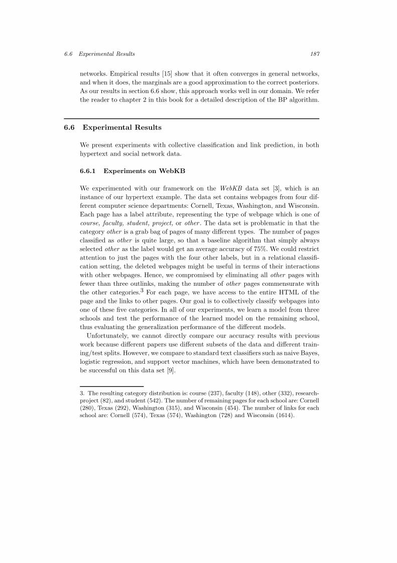
We experimented with our framework on the WebKB data set [3], which is aninstance of our hypertext example. The data set contains webpages from four dif-ferent computer science departments: Cornell, Texas, Washington, and Wisconsin.Each page has a label attribute, representing the type of webpage which is one ofcourse, faculty, student, project, or other . The data set is problematic in that thecategory other is a grab bag of pages of many different types. The number of pagesclassified as other is quite large, so that a baseline algorithm that simply alwaysselected other as the label would get an average accuracy of 75%. We could restrictattention to just the pages with the four other labels, but in a relational classifi-cation setting, the deleted webpages might be useful in terms of their interactionswith other webpages. Hence, we compromised by eliminating all other pages withfewer than three outlinks, making the number of other pages commensurate withthe other categories.3 For each page, we have access to the entire HTML of thepage and the links to other pages. Our goal is to collectively classify webpages intoone of these five categories. In all of our experiments, we learn a model from threeschools and test the performance of the learned model on the remaining school,thus evaluating the generalization performance of the different models.

Unfortunately, we cannot directly compare our accuracy results with previouswork because different papers use different subsets of the data and different train-ing/test splits. However, we compare to standard text classifiers such as naive Bayes,logistic regression, and support vector machines, which have been demonstrated tobe successful on this data set [9].

3. The resulting category distribution is: course (237), faculty (148), other (332), research-project (82), and student (542). The number of remaining pages for each school are: Cornell(280), Texas (292), Washington (315), and Wisconsin (454). The number of links for eachschool are: Cornell (574), Texas (574), Washington (728) and Wisconsin (1614).


0

0.05

0.1

0.15

0.2

0.25

0.3

0.35

Naïve Bayes Svm Logistic

Tes

tE

rro

r

Words Words+Meta

0

0.05

0.1

0.15

0.2

0.25

0.3

0.35

Cor Tex Wash Wisc AVG

Tes

tE

rro

r

Logistic Link Section Link+Section

(a) (b)

Figure 6.2 (a) Comparison of Naive Bayes, Svm, and Logistic on WebKB, withand without metadata features. (Only averages over the four schools are shownhere.) (b) Flat versus collective classification on WebKB: flat logistic regressionwith metadata, and three different relational models: Link, Section, and a combinedSection+Link. Collectively classifying page labels (Link, Section, Section+Link)consistently reduces the error over the flat model (logistic regression) on all schools,for all three relational models.

6.6.1.1 Flat Models

The simplest approach we tried predicts the categories based on just the text contenton the webpage. The text of the webpage is represented using a set of binaryattributes that indicate the presence of different words on the page. We found thatstemming and feature selection did not provide much benefit and simply prunedwords that appeared in fewer than three documents in each of the three schoolsin the training data. We also experimented with incorporating metadata: wordsappearing in the title of the page, in anchors of links to the page, and in thelast header before a link to the page [24]. Note that metadata, although mostlyoriginating from pages linking into the considered page, are easily incorporated asfeatures, i.e., the resulting classification task is still flat feature-based classification.Our first experimental setup compares three well-known text classifiers — Naive

Bayes, linear support vector machines 4 (Svm), and logistic regression (Logistic)— using words and metawords. The results, shown in figure 6.2(a), show that thetwo discriminative approaches outperform Naive Bayes. Logistic and Svm give verysimilar results. The average error over the four schools was reduced by around 4%by introducing the metadata attributes.

4. We trained one-against-others SVM for each category and during testing, picked thecategory with the largest margin.


6.6.1.2 Relational Models

Incorporating metadata gives a significant improvement, but we can take additionaladvantage of the correlation in labels of related pages by classifying them collec-tively. We want to capture these correlations in our model and use them for trans-mitting information between linked pages to provide more accurate classification.We experimented with several relational models. Recall that logistic regression issimply a flat conditional Markov network. All of our relational Markov networksuse a logistic regression model locally for each page.

Our first model captures direct correlations between labels of linked pages. Thesecorrelations are very common in our data: courses and research projects almostnever link to each other; faculty rarely link to each other; students have links toall categories but mostly to courses. The Link model, shown in figure 6.1, capturesthis correlation through links: in addition to the local bag of words and metadataattributes, we introduce a relational clique template over the labels of two pagesthat are linked.

A second relational model uses the insight that a webpage often has internalstructure that allows it to be broken up into sections. For example, a facultywebpage might have one section that discusses research, with a list of links toall of the projects of the faculty member, a second section might contain links tothe courses taught by the faculty member, and a third to his advisees. This patternis illustrated in figure 6.3. We can view a section of a webpage as a fine-grainedversion of Kleinberg’s hub [10] (a page that contains a lot of links to pages of aparticular category). Intuitively, if we have links to two pages in the same section,they are likely to be on similar topics. To take advantage of this trend, we needto enrich our schema with a new relation Section, with attributes Key, Doc (thedocument in which it appears), and Category. We also need to add the attributeSection to Link to refer to the section it appears in. In the RMN, we have two newrelational clique templates. The first contains the label of a section and the labelof the page it is on:

SELECT doc.Category, sec.CategoryFROM Doc doc, Section secWHERE sec.Doc = doc.Key

The second clique template involves the label of the section containing the link andthe label of the target page.

SELECT sec.Category, doc.CategoryFROM Section sec, Link link, Doc docWHERE link.Sec = sec.Key and link.To = doc.Key

The original data set did not contain section labels, so we introduced them usingthe following simple procedure. We defined a section as a sequence of three or morelinks that have the same path to the root in the HTML parse tree. In the trainingset, a section is labeled with the most frequent category of its links. There is a sixth


Figure 6.3 An illustration of the Section model.

category, none, assigned when the two most frequent categories of the links are lessthan a factor of 2 apart. In the entire data set, the breakdown of labels for thesections we found is: course (40), faculty (24), other (187), research.project (11),student (71), and none (17). Note that these labels are hidden in the test data, sothe learning algorithm now also has to learn to predict section labels. Although notour final aim, correct prediction of section labels is very helpful. Words appearingin the last header before the section are used to better predict the section label byintroducing a clique over these words and section labels.

We compared the performance of Link, Section, and Section+Link (a combinedmodel which uses both types of cliques) on the task of predicting webpage labels,relative to the baseline of flat logistic regression with metadata. Our experimentsused MAP estimation with a Gaussian prior on the feature weights with standarddeviation of 0.3. Figure 6.2(b) compares the average error achieved by the differentmodels on the four schools, training on three and testing on the fourth. We seethat incorporating any type of relational information consistently gives significantimprovement over the baseline model. The Link model incorporates more relationalinteractions, but each is a weaker indicator. The Section model ignores links outsideof coherent sections, but each of the links it includes is a very strong indicator. Ingeneral, we see that the Section model performs slightly better. The joint modelis able to combine benefits from both and generally outperforms all of the othermodels. The only exception is for the task of classifying the Wisconsin data. Inthis case, the joint Section+Link model contains many links, as well as some largetightly connected loops, so belief propagation did not converge for a subset of nodes.Hence, the results of the inference, which was stopped at a fixed arbitrary numberof iterations, were highly variable and resulted in lower accuracy.

6.6.1.3 Discriminative vs. Generative

Our last experiment illustrates the benefits of discriminative training in relationalclassification. We compared three models. The Exists+Naive Bayes model is a com-pletely generative model proposed by Getoor et al. [8]. At each page, a naive Bayesmodel generates the words on a page given the page label. A separate generativemodel specifies a probability over the existence of links between pages conditioned


0

0.05

0.1

0.15

0.2

0.25

0.3

0.35

Cor Tex Wash Wisc AVG

Tes

tE

rro

r

Exists+Naïve Bayes Exists+Logistic Link

Figure 6.4 Comparison of generative and discriminative relational models. Ex-

ists+Naive Bayes is completely generative. Exists+Logistic is generative in the links,but locally discriminative in the page labels given the local features (words, meta-words). The Link model is completely discriminative.

on both pages’ labels. We can also consider an alternative Exists+Logistic model thatuses a discriminative model for the connection between page label and words —i.e., uses logistic regression for the conditional probability distribution of page labelgiven words. This model has equivalent expressive power to the naive Bayes modelbut is discriminatively rather than generatively trained. Finally, the Link model isa fully discriminative (undirected) variant we have presented earlier, which uses adiscriminative model for the label given both words and link existence. The results,shown in figure 6.4, show that discriminative training provides a significant im-provement in accuracy: the Link model outperforms Exists+Logistic which in turnoutperforms Exists+Naive Bayes.

As illustrated in table 6.1, the gain in accuracy comes at some cost in trainingtime: for the generative models, parameter estimation is closed form while thediscriminative models are trained using conjugate gradient, where each iterationrequires inference over the unrolled RMN. On the other hand, both types ofmodels require inference when the model is used on new data; the generativemodel constructs a much larger, fully connected network, resulting in significantlylonger testing times. We also note that the situation changes if some of the datais unobserved in the training set. In this case, generative training also requires aniterative procedure (such as the expectation macimation algorihtm (EM)) whereeach iteration uses the significantly more expressive inference.

6.6.2 Experiments on extended WebKB

We collected and manually labeled a new relational data set inspired by WebKB [3].Our data set consists of computer science department webpages from three schools:Stanford, Berkeley, and MIT. A total of 2954 pages are labeled into one of eightcategories: faculty, student, research scientist, staff, research group, research project,


Table 6.1 Average train/test running times (seconds). All runs were done on a700Mhz Pentium III. Training times are averaged over four runs on three schoolseach. Testing times are averaged over four runs on one school each.

Links Links+Section Exists+NB

Training 1530 6060 1

Testing 7 10 100

course, and organization (organization refers to any large entity that is not aresearch group). Owned pages, which are owned by an entity but are not the mainpage for that entity, were manually assigned to that entity. The average distributionof classes across schools is: organization (9%), student (40%), research group (8%),faculty (11%), course (16%), research project (7%), research scientist (5%), andstaff (3%).

We established a set of candidate links between entities based on evidence of arelation between them. One type of evidence for a relation is a hyperlink from anentity page or one of its owned pages to the page of another entity. A second typeof evidence is a virtual link : We assigned a number of aliases to each page usingthe page title, the anchor text of incoming links, and email addresses of the entityinvolved. Mentioning an alias of a page on another page constitutes a virtual link.The resulting set of 7161 candidate links were labeled as corresponding to one offive relation types — advisor (faculty, student), member (research group/project,student/faculty/research scientist), teach (faculty/research scientist/staff, course),TA (student, course), part-of (research group, research project) — or “none,”denoting that the link does not correspond to any of these relations.

The observed attributes for each page are the words on the page itself and the“metawords” on the page — the words in the title, section headings, anchors to thepage from other pages. For links, the observed attributes are the anchor text, textjust before the link (hyperlink or virtual link), and the heading of the section inwhich the link appears.

Our task is to predict the relation type, if any, for all the candidate links. Wetried two settings for our experiments: with page categories observed (in the testdata) and page categories unobserved. For all our experiments, we trained on twoschools and tested on the remaining school.

Observed entity labels We first present results for the setting with observedpage categories. Given the page labels, we can rule out many impossible relations;the resulting label breakdown among the candidate links is: none (38%), member(34%), part-of (4%), advisor (11%), teach (9%), TA (5%).

There is a huge range of possible models that one can apply to this task. Weselected a set of models that we felt represented some range of patterns thatmanifested in the data.

Link-Flat is our baseline model, predicting links one at a time using multinomiallogistic regression. This is a strong classifier, and its performance is competitive


0.7

0.75

0.8

0.85

0.9

0.95

ber mit sta ave

Acc

urac

yFlatTriadSectionSection & Triad

0.6

0.65

0.7

0.75

0.8

0.85

ber mit sta ave

Acc

ura

cy

FlatNeigh

(a) (b)

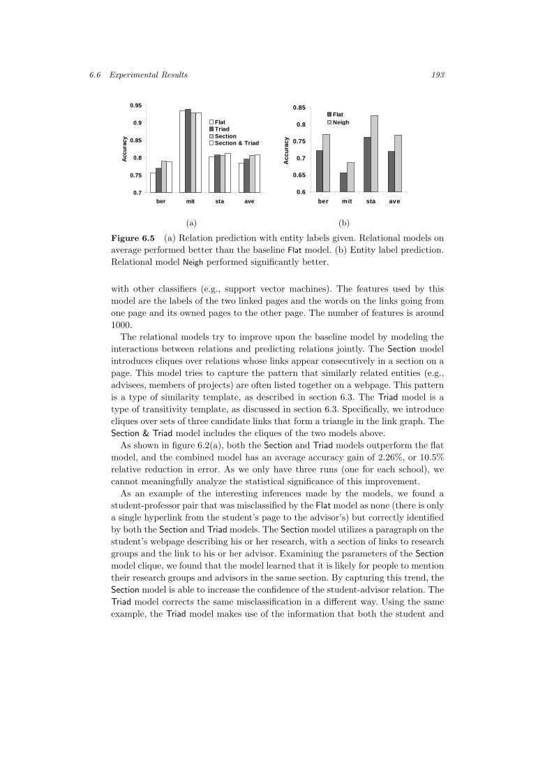
Figure 6.5 (a) Relation prediction with entity labels given. Relational models onaverage performed better than the baseline Flat model. (b) Entity label prediction.Relational model Neigh performed significantly better.

with other classifiers (e.g., support vector machines). The features used by thismodel are the labels of the two linked pages and the words on the links going fromone page and its owned pages to the other page. The number of features is around1000.

The relational models try to improve upon the baseline model by modeling theinteractions between relations and predicting relations jointly. The Section modelintroduces cliques over relations whose links appear consecutively in a section on apage. This model tries to capture the pattern that similarly related entities (e.g.,advisees, members of projects) are often listed together on a webpage. This patternis a type of similarity template, as described in section 6.3. The Triad model is atype of transitivity template, as discussed in section 6.3. Specifically, we introducecliques over sets of three candidate links that form a triangle in the link graph. TheSection & Triad model includes the cliques of the two models above.

As shown in figure 6.2(a), both the Section and Triad models outperform the flatmodel, and the combined model has an average accuracy gain of 2.26%, or 10.5%relative reduction in error. As we only have three runs (one for each school), wecannot meaningfully analyze the statistical significance of this improvement.

As an example of the interesting inferences made by the models, we found astudent-professor pair that was misclassified by the Flat model as none (there is onlya single hyperlink from the student’s page to the advisor’s) but correctly identifiedby both the Section and Triad models. The Section model utilizes a paragraph on thestudent’s webpage describing his or her research, with a section of links to researchgroups and the link to his or her advisor. Examining the parameters of the Section

model clique, we found that the model learned that it is likely for people to mentiontheir research groups and advisors in the same section. By capturing this trend, theSection model is able to increase the confidence of the student-advisor relation. TheTriad model corrects the same misclassification in a different way. Using the sameexample, the Triad model makes use of the information that both the student and


0.45

0.5

0.55

0.6

0.65

0.7

0.75

ber mit sta ave

P/R

Bre

akev

en P

oin

t

Phased (Flat/Flat)Phased (Neigh/Flat)Phased (Neigh/Sec)Joint+NeighJoint+Neigh+Sec

Figure 6.6 Relation prediction without entity labels. Relational models performedbetter most of the time, even though there are schools in which some modelsperformed worse.

the teacher belong to the same research group, and the student TAed a class taughtby his advisor. It is important to note that none of the other relations are observedin the test data, but rather the model bootstraps its inferences.

Unobserved entity labels When the labels of pages are not known duringrelations prediction, we cannot rule out possible relations for candidate links basedon the labels of participating entities. Thus, we have many more candidate links thatdo not correspond to any of our relation types (e.g., links between an organizationand a student). This makes the existence of relations a very low-probability event,with the following breakdown among the potential relations: none (71%), member(16%), part-of (2%), advisor (5%), teach (4%), TA (2%). In addition, when weconstruct a Markov network in which page labels are not observed, the networkis much larger and denser, making the (approximate) inference task much harder.Thus, in addition to models that try to predict page entity and relation labelssimultaneously, we also tried a two-phase approach, where we first predict pagecategories, and then use the predicted labels as features for the model that predictsrelations.

For predicting page categories, we compared two models. The Entity-Flat modelis a multinomial logistic regression that uses words and “metawords” from the pageand its owned pages in separate “bags” of words. The number of features is roughly10, 000. The Neighbors model is a relational model that exploits another type ofsimilarity template: pages with similar URLs often belong to the same category ortightly linked categories (research group/project, professor/course). For each page,two pages with URLs closest in edit distance are selected as “neighbors,” and weintroduced pairwise cliques between “neighboring” pages. Figure 6.5(b) shows thatthe Neighbors model clearly outperforms the Flat model across all schools, by anaverage of 4.9% accuracy gain.


0.4

0.45

0.5

0.55

0.6

0.65

0.7

0.75

10% observed 25% observed 50% observed

ave

p/r

brea

keve

npo

int

flatcompatibility

0.4

0.45

0.5

0.55

0.6

0.65

0.7

0.75

DD JL TX 67 FG LM BC SS

ave

p/r

brea

keve

npo

int

flatcompatibility

(a) (b)

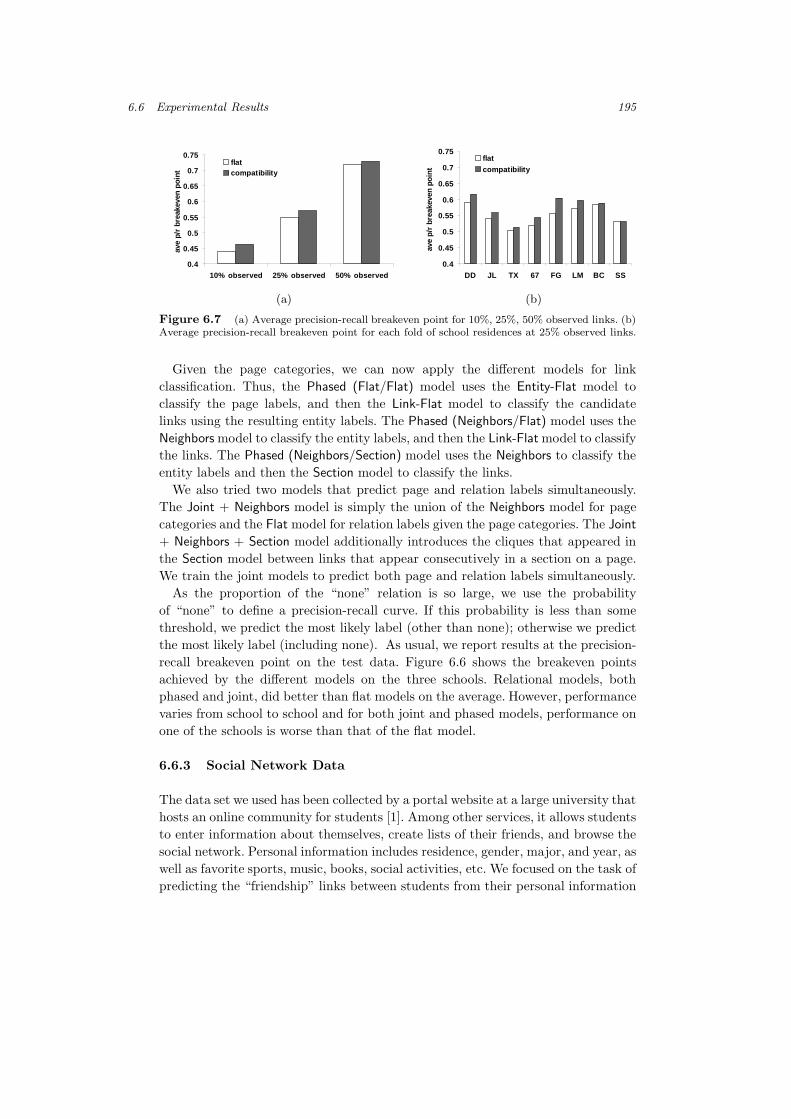
Figure 6.7 (a) Average precision-recall breakeven point for 10%, 25%, 50% observed links. (b)Average precision-recall breakeven point for each fold of school residences at 25% observed links.

Given the page categories, we can now apply the different models for linkclassification. Thus, the Phased (Flat/Flat) model uses the Entity-Flat model toclassify the page labels, and then the Link-Flat model to classify the candidatelinks using the resulting entity labels. The Phased (Neighbors/Flat) model uses theNeighbors model to classify the entity labels, and then the Link-Flat model to classifythe links. The Phased (Neighbors/Section) model uses the Neighbors to classify theentity labels and then the Section model to classify the links.

We also tried two models that predict page and relation labels simultaneously.The Joint + Neighbors model is simply the union of the Neighbors model for pagecategories and the Flat model for relation labels given the page categories. The Joint

+ Neighbors + Section model additionally introduces the cliques that appeared inthe Section model between links that appear consecutively in a section on a page.We train the joint models to predict both page and relation labels simultaneously.

As the proportion of the “none” relation is so large, we use the probabilityof “none” to define a precision-recall curve. If this probability is less than somethreshold, we predict the most likely label (other than none); otherwise we predictthe most likely label (including none). As usual, we report results at the precision-recall breakeven point on the test data. Figure 6.6 shows the breakeven pointsachieved by the different models on the three schools. Relational models, bothphased and joint, did better than flat models on the average. However, performancevaries from school to school and for both joint and phased models, performance onone of the schools is worse than that of the flat model.

6.6.3 Social Network Data

The data set we used has been collected by a portal website at a large university thathosts an online community for students [1]. Among other services, it allows studentsto enter information about themselves, create lists of their friends, and browse thesocial network. Personal information includes residence, gender, major, and year, aswell as favorite sports, music, books, social activities, etc. We focused on the task ofpredicting the “friendship” links between students from their personal information


and a subset of their links. We selected students living in sixteen different residencesor dorms and restricted the data to the friendship links only within each residence,eliminating interresidence links from the data to generate independent training/testsplits. Each residence has about fifteen to twenty-five students and an averagestudent lists about 25% of his or her housemates as friends.

We used an eight-fold train-test split, where we trained on fourteen residences andtested on two. Predicting links between two students from just personal informationalone is a very difficult task, so we tried a more realistic setting, where someproportion of the links is observed in the test data, and can be used as evidence forpredicting the remaining links. We used the following proportions of observed linksin the test data: 10%, 25%, and 50%. The observed links were selected at random,and the results we report are averaged over five folds of these random selectiontrials.

Using just the observed portion of links, we constructed the following flat features:for each student, the proportion of students in the residence that list him/her andthe proportion of students he/she lists; for each pair of students, the proportion ofother students they have as common friends. The values of the proportions werediscretized into four bins. These features capture some of the relational structureand dependencies between links: Students who list (or are listed by) many friendsin the observed portion of the links tend to have links in the unobserved portion aswell. More importantly, having friends in common increases the likelihood of a linkbetween a pair of students.

The Flat model uses logistic regression with the above features as well as personalinformation about each user. In addition to the individual characteristics of the twopeople, we also introduced a feature for each match of a characteristic; for example,both people are computer science majors or both are freshmen.

The Compatibility model uses a type of similarity template, introducing cliquesbetween each pair of links emanating from each person. Similarly to the Flat model,these cliques include a feature for each match of the characteristics of the twopotential friends. This model captures the tendency of a person to have friendswho share many characteristics (even though the person might not possess them).For example, a student may be friends with several computer science majors, eventhough he is not a CS major himself. We also tried models that used transitivitytemplates, but the approximate inference with 3-cliques often failed to converge orproduced erratic results.

Figure 6.7(a) compares the average precision-recall breakpoint achieved by thedifferent models at the three different settings of observed links. Figure 6.7(b) showsthe performance on each of the eight folds containing two residences each. Usinga paired t -test, the Compatibility model outperforms Flat with p-values 0.0036,0.00064, and 0.054 respectively.

6.7 Discussion and Conclusions 197

6.7 Discussion and Conclusions

We propose an approach for collective classification and link prediction in relationaldomains. Our approach provides a coherent probabilistic foundation for the processof collective prediction, where we want to classify multiple entities and links,exploiting the interactions between the variables. We have shown that we canexploit a very rich set of relational patterns in classification, significantly improvingthe classification accuracy over standard flat classification.

We show that the use of a probabilistic model over link graphs allows us torepresent and exploit interesting subgraph patterns in the link graph. Specifically,we have found two types of patterns that seem to be beneficial in several places.Similarity templates relate the classification of links or objects that share a certaingraph-based property (e.g., links that share a common endpoint). Transitivitytemplates relate triples of objects and links organized in a triangle.

Our results use a set of relational patterns that we have discovered to be usefulin the domains that we have considered. However, many other rich and interestingpatterns are possible. Thus, in the relational setting, even more so than in simplertasks, the issue of feature construction is critical. It is therefore important to explorethe problem of automatic feature induction, as in [4].

Finally, we believe that the problem of modeling link graphs has numerousother applications, including analyzing communities of people and the hierarchicalstructure of organizations, identifying people or objects that play certain key roles,predicting current and future interactions, and more.

References

[1] L. Adamic, O. Buyukkokten, and E. Adar. A social network caught in the web.http://www.hpl.hp.com/shl/papers/social/, 2002.

[2] S. Chakrabarti, B. Dom, and P. Indyk. Enhanced hypertext categorizationusing hyperlinks. In Proceedings of ACM International Conference on Man-agement of Data, 1998.

[3] M. Craven, D. DiPasquo, D. Freitag, A. McCallum, T. Mitchell, K. Nigam,and S. Slattery. Learning to extract symbolic knowledge from the World WideWeb. In Proceedings of the National Conference on Artificial Intelligence, 1998.

[4] S. Della Pietra, V. Della Pietra, and J. Lafferty. Inducing features of randomfields. IEEE Transactions on Pattern Analysis and Machine Intelligence, 19(4):380–393, 1997.

[5] L. Egghe and R. Rousseau. Introduction to Informetrics. Elsevier, Amsterdam,1990.

[6] N. Friedman, L. Getoor, D. Koller, and A. Pfeffer. Learning probabilisticrelational models. In Proceedings of the International Joint Conference on


Artificial Intelligence, 1999.

[7] L. Getoor, N. Friedman, D. Koller, and B. Taskar. Learning probabilisticmodels of relational structure. In Proceedings of the International Conferenceon Machine Learning, 2001.

[8] L. Getoor, E. Segal, B. Taskar, and D. Koller. Probabilistic models of textand link structure for hypertext classification. In Proceedings of the IJCAI01Workshop on Text Learning: Beyond Supervision, 2001.

[9] T. Joachims. Transductive inference for text classification using support vectormachines. In Proceedings of the International Conference on Machine Learning,1999.

[10] J. M. Kleinberg. Authoritative sources in a hyperlinked environment. Journalof the ACM, 46(5):604–632, 1999.

[11] D. Koller and A. Pfeffer. Probabilistic frame-based systems. In Proceedingsof the National Conference on Artificial Intelligence, 1998.

[12] F. Kschischang and B. Frey. Iterative decoding of compound codes byprobability propagation in graphical models. IEEE Journal of Selected Areasin Communications, 16(2):219–230, 1998.

[13] J. Lafferty, A. McCallum, and F. Pereira. Conditional random fields: Prob-abilistic models for segmenting and labeling sequence data. In Proceedings ofthe International Conference on Machine Learning, 2001.

[14] R. McEliece, D. MacKay, and J. Cheng. Turbo decoding as an instance ofPearl’s ‘belief propagation’ algorithm. IEEE Journal on Selected Areas inCommunications, 16(2):140–152, 1998.

[15] K. P. Murphy, Y. Weiss, and M. I. Jordan. Loopy belief propagation forapproximate inference: an empirical study. In Proceedings of the Conferenceon Uncertainty in Artificial Intelligence, 1999.

[16] J. Neville and D. Jensen. Iterative classification in relational data. InProceedings of the AAAI-2000 Workshop on Learning Statistical Models fromRelational Data, 2000.

[17] J. Pearl. Probabilistic Reasoning in Intelligent Systems. Morgan Kaufmann,San Francisco, 1988.

[18] F. Sha and F. Pereira. Shallow parsing with conditional random fields. InProceedings of Human Language Technology Conference and North AmericanChapter of the Association for Computational Linguistics, 2003.

[19] S. Slattery and T. Mitchell. Discovering test set regularities in relationaldomains. In Proceedings of the International Conference on Machine Learning,2000.

[20] B. Taskar, E. Segal, and D. Koller. Probabilistic classification and clusteringin relational data. In Proceedings of the International Joint Conference onArtificial Intelligence, 2001.

References 199

[21] B. Taskar, P. Abbeel, and D. Koller. Discriminative probabilistic models forrelational data. In Proceedings of the Conference on Uncertainty in ArtificialIntelligence, 2002.

[22] B. Taskar, M. Wong, P. Abbeel, and D. Koller. Link prediction in relationaldata. In Proceedings of Neural Information Processing Systems, 2003.

[23] V. Vapnik. The Nature of Statistical Learning Theory. Springer-Verlag, NewYork, 1995.

[24] Y. Yang, S. Slattery, and R. Ghani. A study of approaches to hypertextcategorization. Journal of Intelligent Information Systems, 18(2):219–241,2002.

6 relational markov networks - university of central...

Documents