6.- supervised neural networks: multilayer perceptron€¦ · supervised neural networks:...

1

CVG-UPM C

OM

PU

TE

R V

ISIO

N

Machine Learning and Neural Networks P. Campoy P. Campoy

Machine Learning & Neural Networks

6.- Supervised Neural Networks:

Multilayer Perceptron by

Pascual Campoy Grupo de Visión por Computador

U.P.M. - DISAM

CVG-UPM

CO

MP

UT

ER

VIS

ION


topics

  Artificial Neural Networks

  Perceptron and the MLP structure

  The Back-Propagation learning algorithm

  MLP features and drawbacks

  The auto-encoder

2

CVG-UPM C

OM

PU

TE

R V

ISIO

N


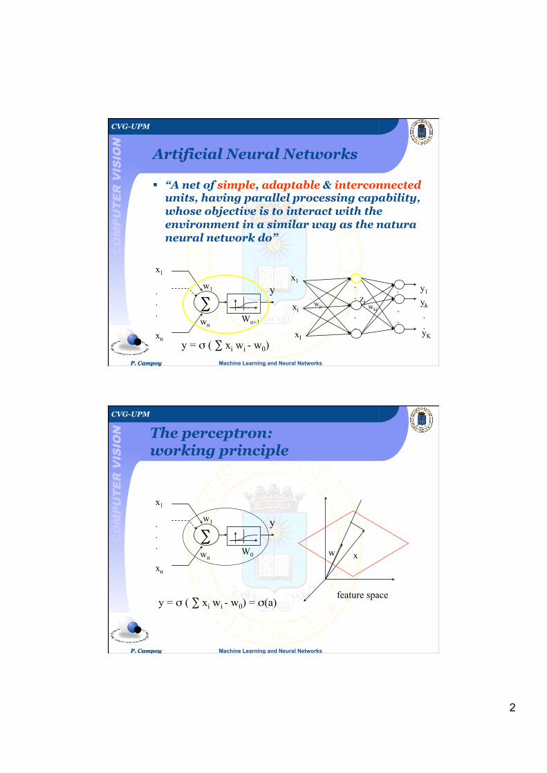
Artificial Neural Networks

  “A net of simple, adaptable & interconnected units, having parallel processing capability, whose objective is to interact with the environment in a similar way as the natura neural network do”

y = σ ( ∑ xi wi - w0)

x1 . . . xn

∑w1

wn

y

Wn+1

.

.

.

.

y1

yK

.

.

.

yk

.

.

.

x1

xI

xi

.

. .

zj wji wkj

CVG-UPM

CO

MP

UT

ER

VIS

ION


The perceptron: working principle

feature space

w x

y = σ ( ∑ xi wi - w0) = σ(a)

x1 . . . xn

∑w1

wn

y

W0

3

CVG-UPM C

OM

PU

TE

R V

ISIO

N


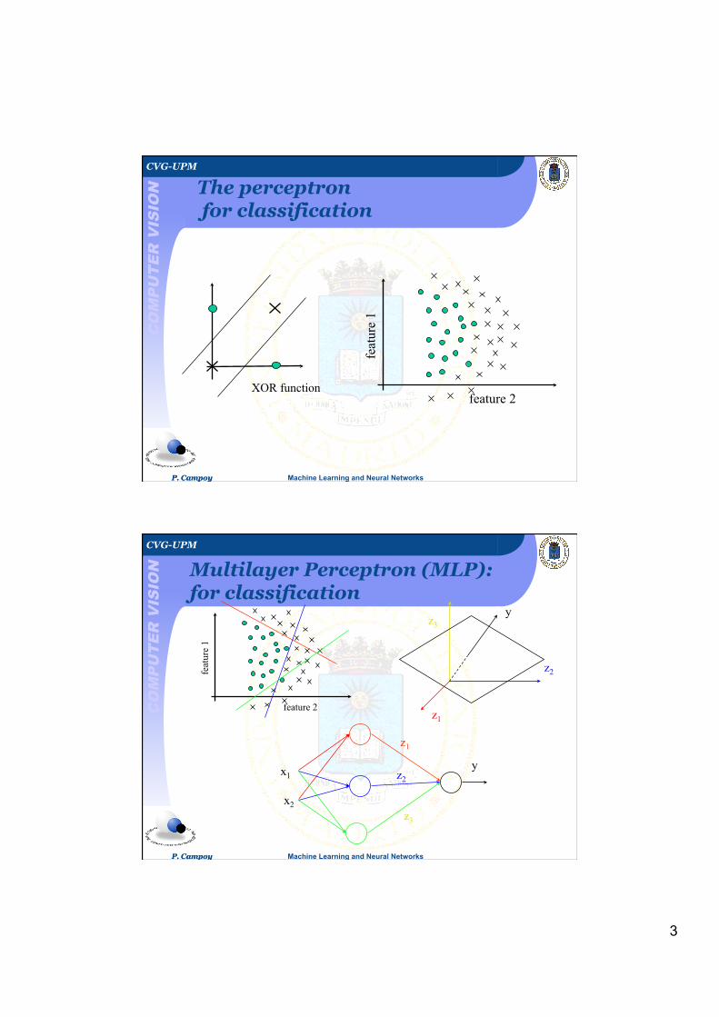
The perceptron for classification

XOR function fe

atur

e 1

feature 2

CVG-UPM

CO

MP

UT

ER

VIS

ION


Multilayer Perceptron (MLP): for classification

y z3

z2

z1

y

feat

ure

1

feature 2

x1

x2

z1

z2

z3

4

CVG-UPM C

OM

PU

TE

R V

ISIO

N


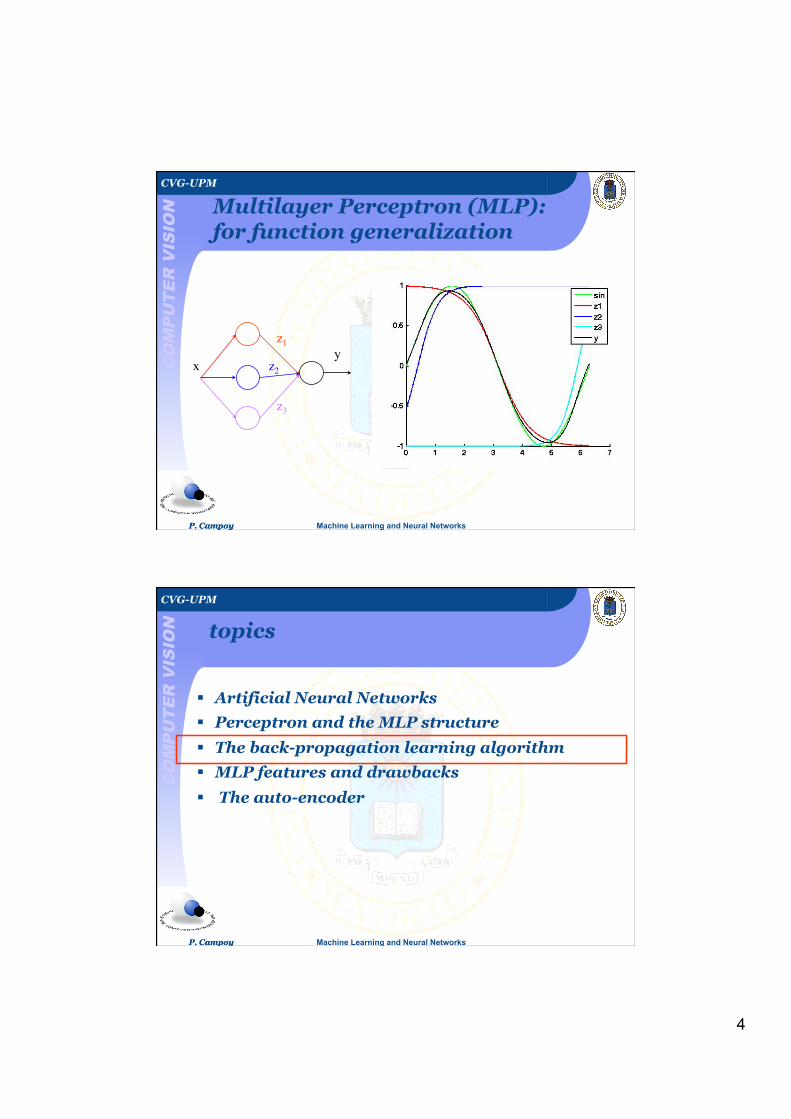
Multilayer Perceptron (MLP): for function generalization

x

z1

z2

z3

y

CVG-UPM

CO

MP

UT

ER

VIS

ION


topics



  The back-propagation learning algorithm



5

CVG-UPM C

OM

PU

TE

R V

ISIO

N


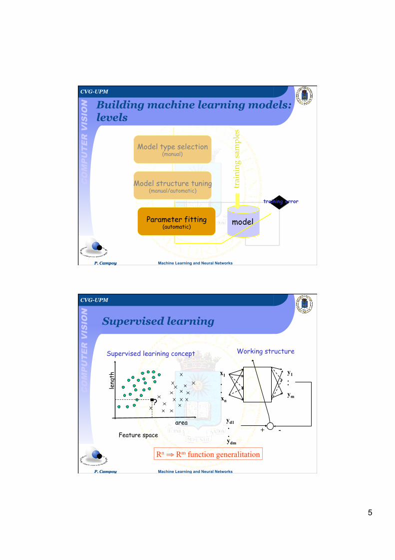
Building machine learning models: levels

Model structure tuning (manual/automatic)

Model type selection (manual)

model Parameter fitting (automatic)

!

trai

ning

sam

ples!

training error

CVG-UPM

CO

MP

UT

ER

VIS

ION


Supervised learning

area

leng

th

Feature space

?

Supervised learining concept Working structure

y1 . . ym

.

. xn

x1

yd1

ydm

+ - . .

Rn ⇒ Rm function generalitation

6

CVG-UPM C

OM

PU

TE

R V

ISIO

N


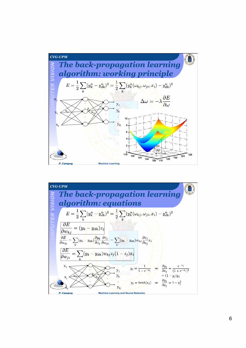
The back-propagation learning algorithm: working principle

.

.

.

.

y1

yK

.

.

.

yk

.

.

.

x1

xI

xi

.

. .

zj wji wkj

CVG-UPM

CO

MP

UT

ER

VIS

ION


The back-propagation learning algorithm: equations

.

.

.

.

y1

yK

.

.

.

yk

.

.

.

x1

xI

xi

.

. .

zj wji wkj

7

CVG-UPM C

OM

PU

TE

R V

ISIO

N


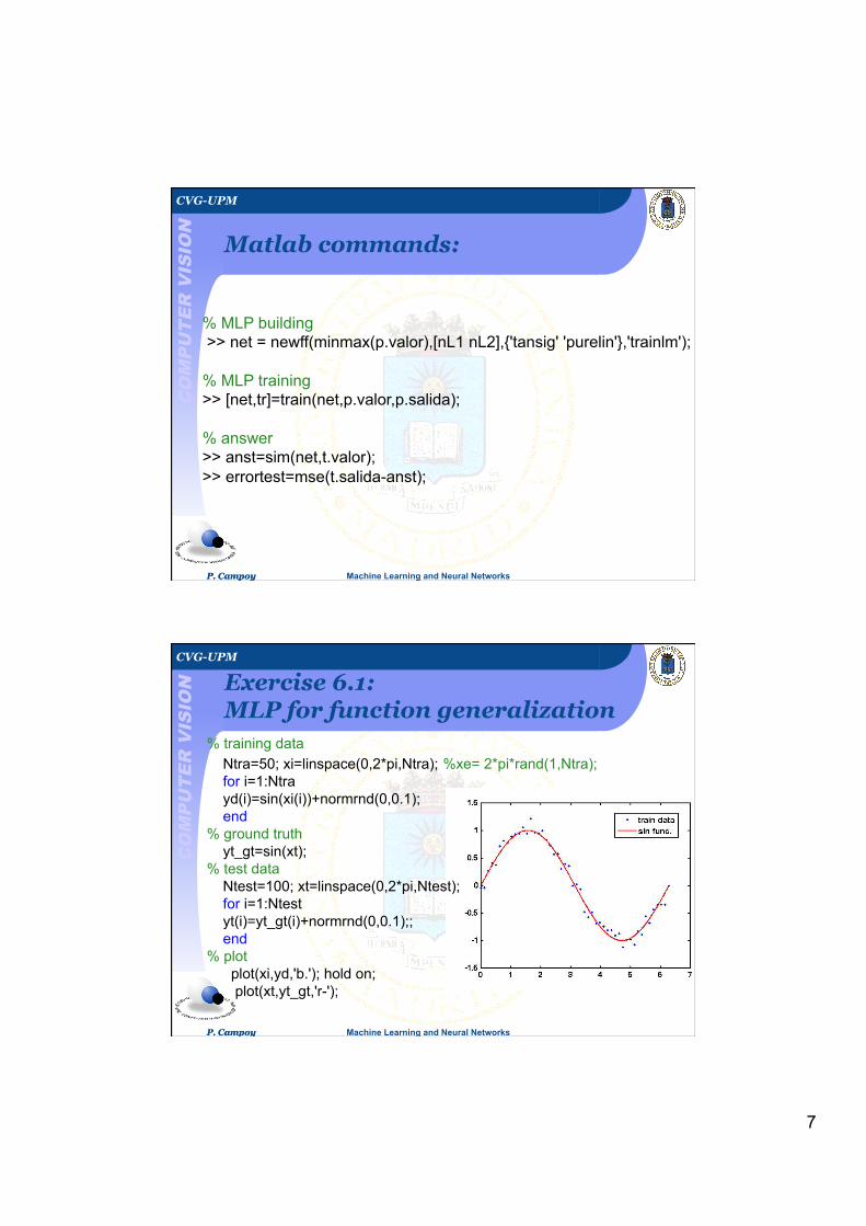
Matlab commands:

% MLP building >> net = newff(minmax(p.valor),[nL1 nL2],{'tansig' 'purelin'},'trainlm'); % MLP training >> [net,tr]=train(net,p.valor,p.salida); % answer >> anst=sim(net,t.valor); >> errortest=mse(t.salida-anst);

CVG-UPM

CO

MP

UT

ER

VIS

ION


Exercise 6.1: MLP for function generalization

% training data Ntra=50; xi=linspace(0,2*pi,Ntra); %xe= 2*pi*rand(1,Ntra); for i=1:Ntra yd(i)=sin(xi(i))+normrnd(0,0.1); end % ground truth yt_gt=sin(xt); % test data Ntest=100; xt=linspace(0,2*pi,Ntest); for i=1:Ntest yt(i)=yt_gt(i)+normrnd(0,0.1);; end % plot plot(xi,yd,'b.'); hold on; plot(xt,yt_gt,'r-');

8

CVG-UPM C

OM

PU

TE

R V

ISIO

N


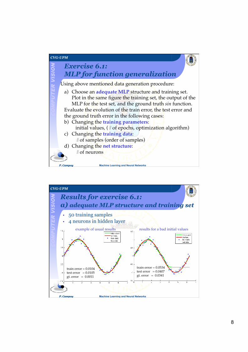
Exercise 6.1: MLP for function generalization

a)  Choose an adequate MLP structure and training set.!Plot in the same figure the training set, the output of the!MLP for the test set, and the ground truth sin function.!

Evaluate the evolution of the train error, the test error and!the ground truth error in the following cases:!b)  Changing the training parameters:!! initial values, (# of epochs, optimization algorithm)!

c)  Changing the training data:!! # of samples (order of samples)!

d)  Changing the net structure:!! # of neurons!

Using above mentioned data generation procedure: !

CVG-UPM

CO

MP

UT

ER

VIS

ION


results for a bad initial values!

Results for exercise 6.1: a) adequate MLP structure and training set •  50 training samples •  4 neurons in hidden layer

train error = 0.0104!test error = 0.0105!gt. error = 0.0011!

train error = 0.0534!test error = 0.0407!gt. error = 0.0341!

example of usual results!

9

CVG-UPM C

OM

PU

TE

R V

ISIO

N


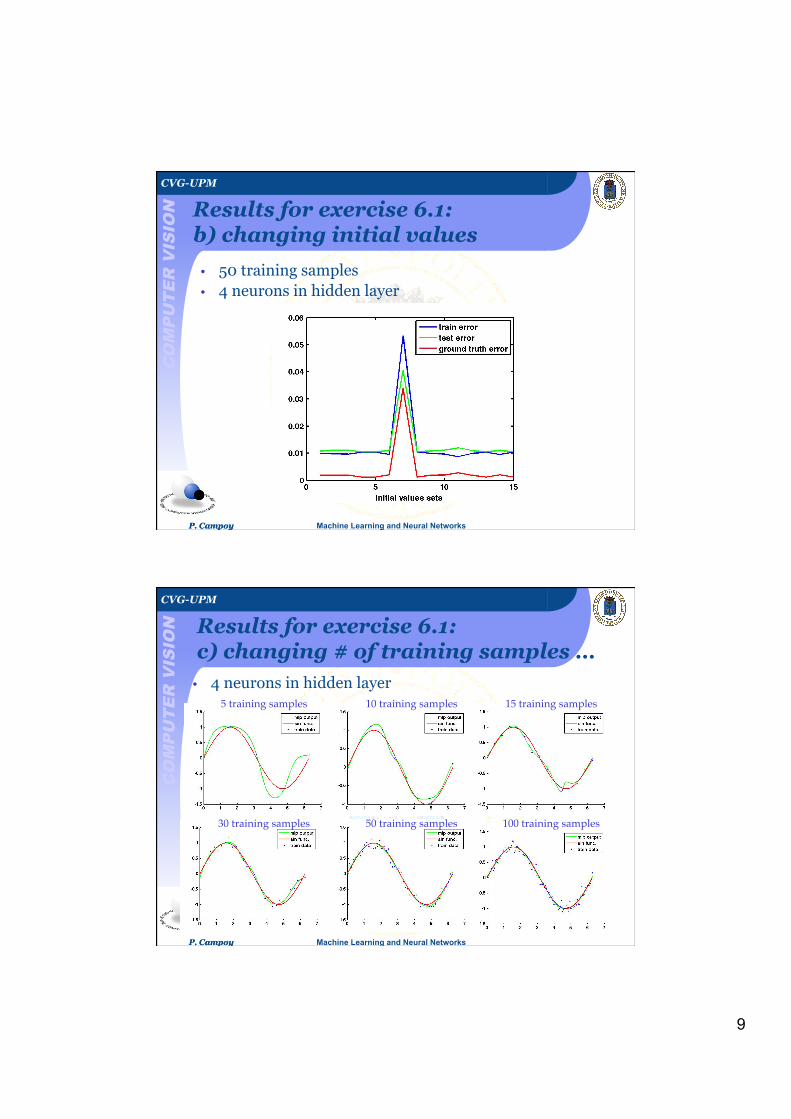
Results for exercise 6.1: b) changing initial values

•  50 training samples •  4 neurons in hidden layer

CVG-UPM

CO

MP

UT

ER

VIS

ION


Results for exercise 6.1: c) changing # of training samples … •  4 neurons in hidden layer

5 training samples! 10 training samples! 15 training samples!

100 training samples!50 training samples!30 training samples!

10

CVG-UPM C

OM

PU

TE

R V

ISIO

N


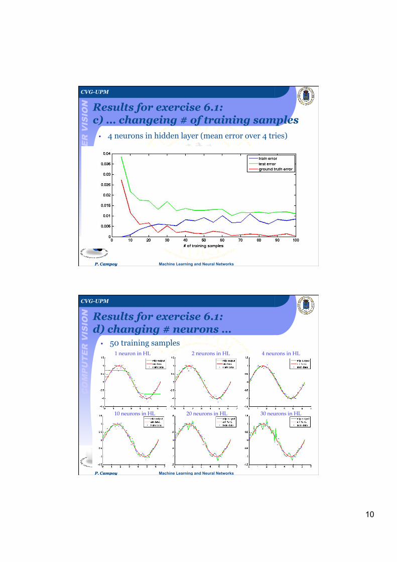
Results for exercise 6.1: c) … changeing # of training samples •  4 neurons in hidden layer (mean error over 4 tries)

CVG-UPM

CO

MP

UT

ER

VIS

ION


Results for exercise 6.1: d) changing # neurons … •  50 training samples

1 neuron in HL! 2 neurons in HL! 4 neurons in HL!

30 neurons in HL!20 neurons in HL!10 neurons in HL!

11

CVG-UPM C

OM

PU

TE

R V

ISIO

N


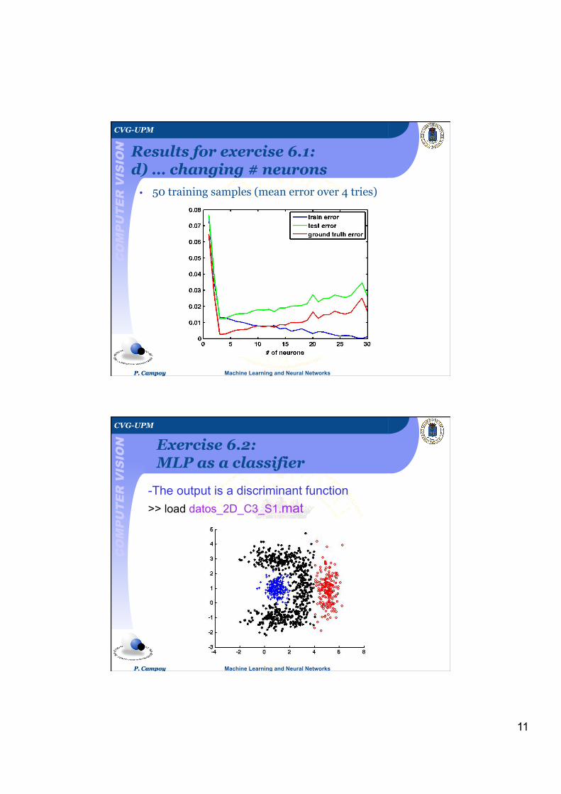
Results for exercise 6.1: d) … changing # neurons •  50 training samples (mean error over 4 tries)

CVG-UPM

CO

MP

UT

ER

VIS

ION


Exercise 6.2: MLP as a classifier

- The output is a discriminant function >> load datos_2D_C3_S1.mat

12

CVG-UPM C

OM

PU

TE

R V

ISIO

N


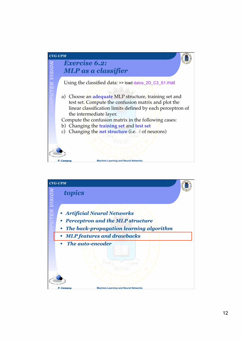
Exercise 6.2: MLP as a classifier

a)  Choose an adequate MLP structure, training set and test set. Compute the confusion matrix and plot the linear classification limits defined by each perceptron of the intermediate layer.!

Compute the confusion matrix in the following cases:!b)  Changing the training set and test set!c)  Changing the net structure (i.e. # of neurons)!

Using the classified data: >> load datos_2D_C3_S1.mat!

CVG-UPM

CO

MP

UT

ER

VIS

ION


topics






13

CVG-UPM C

OM

PU

TE

R V

ISIO

N


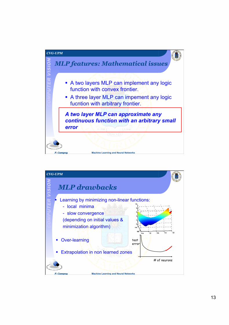
MLP features: Mathematical issues

  A two layers MLP can implement any logic function with convex frontier.

  A three layer MLP can impement any logic fucntion with arbitrary frontier.

A two layer MLP can approximate any continuous function with an arbitrary small error

CVG-UPM

CO

MP

UT

ER

VIS

ION


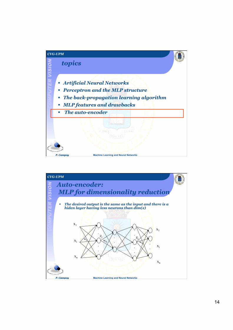
MLP drawbacks

  Learning by minimizing non-linear functions: -  local minima -  slow convergence (depending on initial values & minimization algorithm)

# of neurons

test error

  Over-learning

  Extrapolation in non learned zones

14

CVG-UPM C

OM

PU

TE

R V

ISIO

N


topics






CVG-UPM

CO

MP

UT

ER

VIS

ION


.

. .

.

.

.

.

x1

xn

xi

.

. zj wji wkj

x1

xn

xi . .

.

.

.

. . zj

wkj

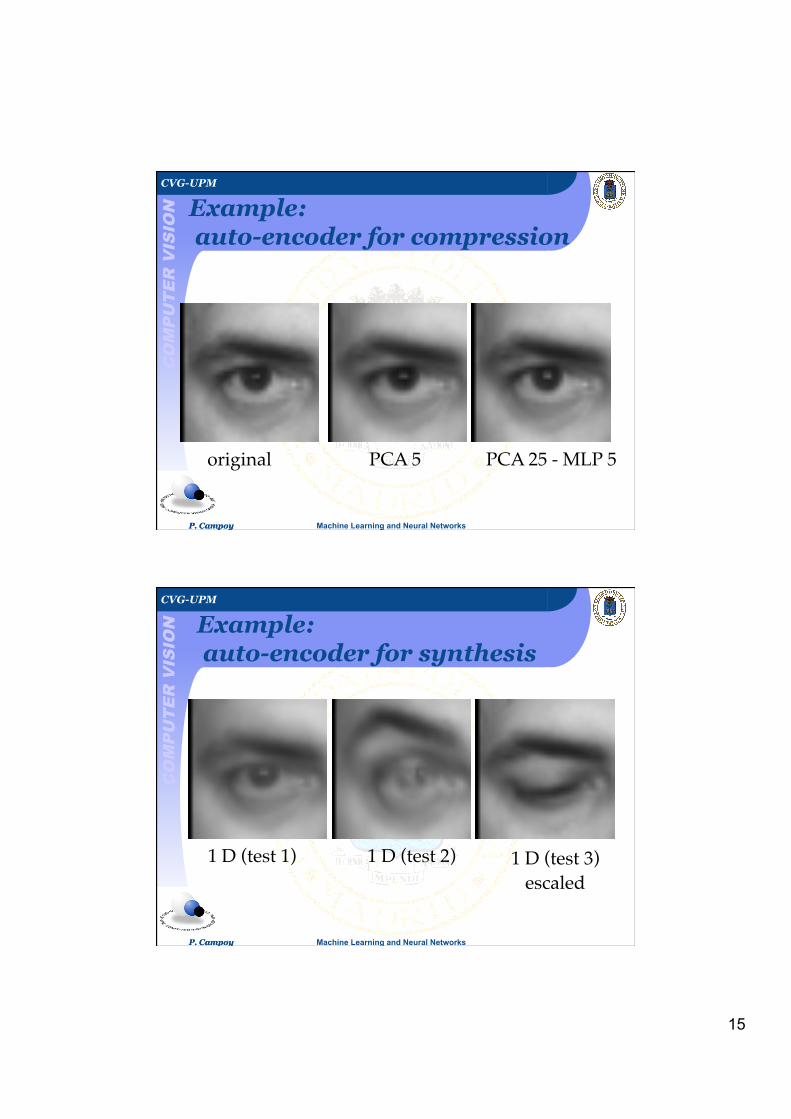
Auto-encoder: MLP for dimensionality reduction

  The desired output is the same as the input and there is a hiden layer having less neurons than dim(x)

15

CVG-UPM C

OM

PU

TE

R V

ISIO

N


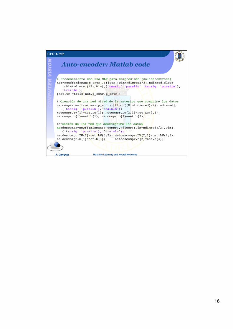
Example: auto-encoder for compression

original! PCA 5! PCA 25 - MLP 5!

CVG-UPM

CO

MP

UT

ER

VIS

ION


Example: auto-encoder for synthesis

1 D (test 1)! 1 D (test 2)! 1 D (test 3)!escaled!

16

CVG-UPM C

OM

PU

TE

R V

ISIO

N


Auto-encoder: Matlab code

% Procesamiento con una MLP para compresioón (salida=entrada)!net=newff(minmax(p_entr),[floor((Dim+ndimred)/2),ndimred,floor

((Dim+ndimred)/2),Dim],{'tansig' 'purelin' 'tansig' 'purelin'}, 'trainlm');!

[net,tr]=train(net,p_entr,p_entr);!!% Creación de una red mitad de la anterior que comprime los datos!netcompr=newff(minmax(p_entr),[floor((Dim+ndimred)/2), ndimred],

{'tansig' 'purelin'},'trainlm');!netcompr.IW{1}=net.IW{1}; netcompr.LW{2,1}=net.LW{2,1};!netcompr.b{1}=net.b{1}; netcompr.b{2}=net.b{2};!!%creación de una red que descomprime los datos!netdescompr=newff(minmax(p_compr),[floor((Dim+ndimred)/2),Dim],

{'tansig' 'purelin'}, 'trainlm');!netdescompr.IW{1}=net.LW{3,2}; netdescompr.LW{2,1}=net.LW{4,3};!netdescompr.b{1}=net.b{3}; netdescompr.b{2}=net.b{4};!

6.- supervised neural networks: multilayer perceptron€¦ · supervised neural networks:...

Documents