6. trading programs - colby college · trading programs 2001 67 6. trading programs ... but...
TRANSCRIPT

Trading Programs
2001 67
6. Trading Programs
Crocker and Dales generally are credited with first proposing that marketableemission permits be used as an incentive mechanism for achieving environmentalgoals.89 The basic approach outlined by Crocker and Dales and later refined byDewees and Harrison is that the environmental authority can issue a fixed number ofmarketable permits to release emissions.90 Through trading, low-cost sources will sellsome of their permits and abate more than they would under a traditional regulatoryapproach, while high-cost sources will buy permits and abate less. The end result,according to the academic design, is the same amount of pollution reduction thatwould be achieved through traditional regulatory approaches, but it is achieved atlower cost.
EPA first applied the concept of marketable emission permits in the mid-1970s as ameans for new sources of emissions to locate in non-attainment areas withoutcausing air quality to worsen. New sources and existing sources that wanted toexpand their facilities were required to offset their emissions by acquiring emissionreduction credits from existing sources. This important but modest beginning wasbased on an interpretation of the Clean Air Act, rather than on a specific statutoryauthority. EPA’s Offset Policy was included in the 1977 amendments to the CleanAir Act statute. In 1980, then-Administrator Hawkins signed a memo that allowedemission averaging between can-coating lines.91
On August 7, 1980, EPA promulgated New Source Review (NSR) and Prevention ofSignificant Deterioration (PSD) rules that allowed netting, a means for sources toavoid PSD and NSR requirements for emission increases due to facility expansion, ifemissions were decreased contemporaneously elsewhere at the facility.92 Under thePSD mandate, this rule included facilities within a plant as a source of emissions aswell as an entire plant as a source of emissions, in what was termed a “dual-sourcedefinition.” Chevron and others challenged this rule, claiming it made modernizationtoo difficult. Eventually the U.S. Supreme Court agreed that states did not need toinclude the dual-source definition in their non-attainment rules. This opened the doorto many of the emission trading programs that exist today.
The 1990 Clean Air Act Amendments authorized a variety of emission tradingsystems. While similar statutory authority to establish effluent permit trading systemsdoes not exist, EPA believes that the Clean Water Act allows effluent trading.Programs of this sort have been operational for several years without legalcontroversy. Pollution permit trading systems now come in a wide variety of forms,and they apply to a large and growing number of sources of pollution that affect thequality of air, water, and land.
Insofar as trading between economic entities is concerned, two main forms of tradingsystems are observed: (1) uncapped emission (or effluent) reductions credit (ERC)systems, and (2) capped allowance systems (also referred to as cap-and-tradesystems). In the case of uncapped systems, pollution limits are rate-based (e.g.,grams per mile for motor vehicles), and sources earn credits by releasing lesspollution than their legal limit or other defined baseline. Under these systems,

The U. S. Experience with Economic Incentives for Protecting the Environment
68 January
emissions can increase with economic growth. By contrast, with capped systems, total emissionsare limited by an overall ceiling that is designed to achieve health or environmental goals, andallowances are allocated to sources in quantities consistent with this ceiling. The formula formaking such allocations will vary from one situation to the next.
A number of the programs described in this chapter involve the right to average emissioncharacteristics of a slate of similar products that are manufactured by one economic entity.Emission averaging is an important mechanism for improving the cost effectiveness ofenvironmental regulation. It can be characterized as intra-firm trading across the product lineswhere it is allowed.
Trading systems, properly designed and applied in appropriate circumstances, can cutcompliance costs, encourage technological development, and create incentives for achievingenvironmental benefits beyond minimum requirements. For trading systems to function well, anumber of requirements must be satisfied. There should be several potential participants in tradesif a functioning market is to be created. Exactly how small a universe of potential participantsthere can be and still have a functioning market is difficult to say, but simulation experimentssuggest that 8−10 participants is a reasonable estimate.93 If sources are dispersed geographically,trading ratios other than one-to-one might have to be imposed to account for wind direction orthe distance between sources to ensure no degradation in environmental quality.
Some pollutants are seasonal in their impact, implying that trades might be allowed only during aportion of the year. Trading might be limited because of a desire to avoid “hot spots” wherepollution concentrations increase. Trading requires that pollution control agencies have theability to monitor emissions (or measure a surrogate to those emissions) reasonably well. Theneed to ensure accountability of trades must not pose unacceptably high transaction costs. Thecommodity to be traded needs to be defined. In general, a well-defined commodity requires abaseline from which to calculate the emission reduction credits (or allowances) that may betraded. Establishing baselines is likely to require good historic data on emissions, input use, etc.In the case of allowance systems, the political will must exist to achieve an allocation ofallowances among competing interests.
Cap-and-trade systems to date have allocated most or all of the allowable emissions under thecap to existing sources, providing allowance set-asides for new sources or using auctions as asafeguard to ensure access to allowances. Initially, environmentalists opposed marketable permittrading because the existence of trading was evidence that sources could make greater reductionsin pollution than were being achieved. In addition, there has been a lingering concern that tradingcould result in localized “hot spots” that had undesirably high levels of pollution. With thesuccess of the Regional Clean Air Incentives Market (RECLAIM) and the Acid Rain Programdescribed later in this chapter, marketable permit trading has become more accepted as a cost-effective means of achieving many environmental goals.
On the other hand, attempts to establish new trading programs often encounter controversy. Forexample, some citizen groups have opposed trading programs for ozone-forming volatile organiccompounds (VOCs). They based their opposition on two basic concerns: (1) the possibility oflocalized toxic pollution “hot spots,” or (2) the ability of the source (or EPA for that matter) toreliably measure emissions to ensure that participants would be held accountable. EPA, inconsultation with environmental justice groups and other stakeholders, is working on guidancefor addressing these environmental justice concerns with trading.

Trading Programs
2001 69
The scope of trading systems is considerable. An emission trading proposal is a centerpiece ofthe Kyoto Protocol for controlling greenhouse gas emissions. Certain Colorado communitieshave created programs to trade the right to own and operate a wood burning stove or fireplace.For a number of years, there was an active program under which refiners could trade lead thatwas used as an additive in gasoline. Heavy-duty truck manufacturers can meet engine emissionstandards by averaging together the emissions performance of all the engines they produce.Programs to trade effluents are operating in selected locations. These particular programs arelikely to be expanded significantly in coming years as a result of a new EPA initiative to improvewater quality in polluted rivers and lakes. Developers whose activities would cause the loss ofwetlands can satisfy mitigation requirements in some areas by purchasing credits from a wetlandmitigation bank.
These and other trading systems for air, water, and land are described in this chapter. Thediscussion begins with a review of trading programs in air emissions, followed by sections onwater effluent trading, land development, and, finally, international trading programs in whichthe United States is involved.
A few basic parameters may be used to characterize trading systems:
1. Scope. Is trading restricted to averaging within a single facility, allowed among facilitiesowned by the same firm, or allowed among firms or facilities under different ownership?
2. Cap. Is there a limit on total emissions or on effluents?
3. Commodity Being Traded. How will the commodity be defined: As allowances for futurepollution, as credits for quantifiable reductions in pollution, as emission characteristics ofproducts, as rights to own and operate products themselves, or as some other definition?
4. Distribution of Tradable Permits. Are the tradable certificates auctioned to the highest bidder,or are they grandfathered to existing sources?
5. Trading Ratio. Is the required trading ratio 1:1 or some greater ratio? Does the trading ratiodepend on the respective location of the sources, season of the year, or other factors?
6. Banking. Can tradable certificates be banked or otherwise reserved for future use?
7. Monitoring. How is credit generation and trading monitored?
8. Environmental Benefit. Is a “set-aside” for the benefit of the environment built into the tradingsystem? For example, each trade could be debited by 10% to yield an environmental benefit.
6.1 Trading in Clean Air Act Programs: An Overview
Since 1990, EPA has significantly expanded the use of trading in Clean Air Act programs.Today, emissions trading is a standard tool of EPA’s air quality program. Although not apanacea for every situation, trading is being used by EPA and states to help solve a variety of airpollution problems. A broad overview of these programs follows. (Some of these programs arediscussed in detail later in this chapter.)
Acid Rain: Perhaps the best-known example of trading is the Acid Rain Program’s system ofmarketable pollution allowances for sulfur dioxide emissions for electric utilities. Enacted as partof the Clean Air Act Amendments of 1990, this cap-and-trade program has been highlysuccessful at achieving cost-effective emissions reductions. The first phase of the program,

The U. S. Experience with Economic Incentives for Protecting the Environment
70 January
which took effect in 1995, reduced annual emissions by 4 million tons. Since then,measurements have shown that rainfall in the eastern United States is as much as 25% lessacidic, some ecosystems in New England are showing signs of recovery, and ambient sulfateconcentrations have been reduced, thus benefiting public health. The second phase of theprogram, beginning in 2000, will more than double the annual emissions reductions achieved bythe first phase over time. The annual cost of the program, once it is fully implemented, isexpected now to be approximately $2 billion, which is about one-half the cost that EPA hadoriginally estimated.
Smog and Other Common Pollutants: EPA is working with states to promote trading and othermarket-based approaches to help achieve national air quality standards for smog, particulates,and other common pollutants that are regulated through national air quality standards. Inaddition, EPA has provided trading opportunities in virtually all federal rules that are aimed atcutting emissions from motor vehicles and fuels. These federal measures are essential to helpingstates meet federal air quality goals.
Under the Clean Air Act, states have primary responsibility for devising pollution controlstrategies for local areas, so states can meet national air quality standards. EPA has issuedguidance to assist states in designing trading and other economic incentive programs, includingeconomic incentives rules and guidance in 1994 (which, at present, are being revised); generalguidance on State Implementation Plans (SIPs) in 1992; and the 1986 emissions trading policystatement. EPA also has assisted states in setting up trading programs, such as California’sRECLAIM cap-and-trade program for sulfur dioxide and nitrogen oxides and the OzoneTransport Commission’s (OTC) program for controlling nitrogen oxide emissions among statesin the Northeast. Through a unique partnership, EPA and the OTC states are jointlyimplementing this NOx budget system for the Northeast, which draws on the experience of theacid rain program.
In 1998, EPA issued a rule that established NOx budgets for many states (the “NOx SIP call”) tocombat the problem of transported ozone pollution in the eastern United States on a broaderscale. To encourage an efficient market-based approach to reducing NOx on a regional basis,EPA simultaneously provided states with a model cap-and-trade rule for utilities and largeindustrial sources. The experiences of the acid rain program and the OTC effort show that thisapproach holds the potential to achieve regional NOx reductions in an efficient and highly cost-effective manner.
In the 1990 Clean Air Act Amendments, Congress called for EPA to help states meet their airquality goals by issuing federal standards to cut emissions from cars, trucks, buses, many typesof non-road engines, and fuels. These rules cut toxic air pollution as well as reduced the amountof air pollutants, which were regulated through air quality standards.
EPA has provided trading opportunities in virtually all of these new standards, building on theearly success of trading in the phased reduction of lead in leaded gasoline during the 1980s.These standards include rules for cleaner burning reformulated gasoline, which now accounts forapproximately 30% of the nation’s gasoline, and the national low-emission vehicle standards forcars and light-duty trucks that will be met nationwide by 2001. Opportunities for averaging,trading, and banking also are provided by new national emissions standards for heavy-dutytrucks and buses, locomotives, heavy-duty off-road engines such as bulldozers, and smallgasoline engines (e.g., those used in lawn and garden equipment).

Trading Programs
2001 71
Another recent example is the landmark Tier II/gasoline sulfur rule that President Clintonannounced in December 1999. This rule would provide compliance flexibility to both vehiclemanufacturers and fuel refiners by allowing them to use averaging, banking, and trading. to Inthe case of automakers, EPA created different “bins” of emissions levels, rather than require asingle NOx emissions standard for each vehicle model. EPA required automakers to achieve afleet average emissions rate of 0.07 grams of NOx per mile (gpm). Automakers whose fleetaverage is below 0.07 gpm could generate credits that they could either use in a later model yearor sell to another auto manufacturer. This rule does allow the production of certain higherpolluting vehicles that consumers desire. However, it also provides a strong incentive for theindustry to develop technology well beyond the 0.07 gpm standard, since any higher pollutingvehicle will have to be offset by a lower polluting one.
Industrial Air Toxics: The 1990 Clean Air Act Amendments called on EPA to establishnational emissions standards to control major industrial sources of toxic air pollution. EPA hasused emissions averaging as one of several ways to provide compliance flexibility in theseindustry-by-industry standards. For example, emissions averaging is permitted by national airtoxics emissions standards for petroleum refining, synthetic organic chemical manufacturing,polymers and resins manufacturing, aluminum production, wood furniture manufacturing,printing and publishing, and a number of other sectors. To avoid shifting risks from one area toanother, toxics averaging is allowed only within individual facilities. With appropriatesafeguards, EPA also has used other methods, including multiple compliance options, to helpprovide flexibility in complying with air toxics rules.
Ozone Layer Depletion: In gradually phasing out the production of chemicals that harm thestratospheric ozone layer, EPA is giving producers and importers the flexibility to tradeallowances. Under the Montreal Protocol, the United States and other developed countries agreedto stop producing and importing CFCs (chlorofluorocarbons) and other chemicals that aredestructive to the ozone layer. By 1996, production of the most harmful ozone-depletingchemicals, including CFCs, virtually ceased in the United States and other developed countries.Additional chemicals are to be phased out in the future. Provided the United States and the worldcommunity maintain their commitment to planned protection efforts, the stratospheric ozonelayer is projected to recover by the middle of the 21st century.
The phase-out of these chemicals is being achieved by using trading rules developed by EPA,rules that have served as a model for programs in other countries. In part because of the flexiblemarket-based approach, the phase-out of CFCs was much less expensive than predicted. In 1988,EPA estimated that a 50% reduction of CFCs by 1998 would cost $3.55 per kilogram. In 1993,the cost for a 100% phase-out by 1996 was reduced to $2.45 per kilogram.
6.2 Foundations of Air Emissions Trading
The first trading of permitted rights to release any type of pollutant in the United States began inthe 1970s as a mechanism to allow economic development in areas that failed to meet ambientair quality standards. EPA gradually broadened the offset policy to include emission bubbles,banking, and netting. These programs are described in the following paragraphs. While many ofthe achievements are modest, EPA’s early efforts in emissions trading are important becausethey provided a foundation and valuable practical experience for the development of moreeffective and cost-effective trading programs such as the Acid Rain Program.
The U. S. Experience with Economic Incentives for Protecting the Environment
72 January
6.2.1 Offset Program
In the mid-1970s, the EPA proposed the “offset” policy that permitted growth in non-attainmentareas, provided that new sources install air pollution control equipment which met LowestAchievable Emission Rate (LAER) standards. These sources also had to offset any excessemissions by acquiring greater emission reductions from other sources in the area. Through thisprocess, growth could be accommodated while maintaining progress toward attaining nationalambient air quality standards.
Of more than 10,000 offset trades (a few of which are described later in this section), over 90%have been in California. Nationwide, about 10% of offset trades are between firms; theremainder are between sources owned by the same firm. Most offset credits are created as aresult of all or part of a facility being closed.
The offset policy, which was included in the 1977 amendments to the Clean Air Act, spawnedthree related programs: bubbles, banking, and netting. The common element in these programs isthe Emission Reduction Credit (ERC), which is generated when sources reduce actual emissionsbelow their permitted emissions and apply to the state for certification of the reduction. To becertified as an ERC, the state must determine that the reduction meets the following criteria: (1)that the reduction is surplus in the sense of not being required by current regulations in the StateImplementation Plan (SIP); (2) that it is enforceable; (3) that it is permanent; and (4) that it isquantifiable. ERCs are normally denominated in terms of the quantity of pollutant in tonsreleased over 1 year. By far the most common method of generating ERCs is closing the sourceor reducing its production. However, ERCs also can be earned by modifying productionprocesses and installing pollution control equipment. Trades of ERCs most often involvestationary sources, although trades involving mobile sources are permitted. States have approveda variety of activities that sources may use to generate offset credits. The South Coast AirQuality Management District (SCAQMD) in California, for example, accepts the scrapping ofolder vehicles and lawn mowers as a means of generating credits. It then applies a formula todetermine the magnitude of air pollution credits for each old car that is scrapped.94
The offset, banking, and netting programs and bubble policy were subject to numerous revisionsbefore being incorporated into EPA’s Final Emission Trading Policy Statement, which wasissued in 1986.95 The Policy Statement addresses trading of ERCs for criteria pollutants such assulfur dioxide, nitrogen oxides, particulate matter, carbon monoxide, and volatile organiccompounds (VOCs) that contribute to the formation of ground-level ozone. The final policystatement responded to public comments that pollutant trading could cause environmentaldamage unless accompanied by safeguards, such as trading ratios greater than 1:1and the use ofair quality modeling in some cases).
6.2.2 Bubble Policy
The bubble policy, established in 1979, allows sources to meet emission limits by treatingmultiple emission points within a facility as if they face a single aggregate emission limit. Theterm bubble was used to connote an imaginary bubble over a source such as a refinery or a steelmill that had several emission points, each with its own emission limit. Within the “bubble,” asource could propose to meet all of its emission control requirements for a criteria pollutant witha mix of controls that is different from those mandated by regulationsas long as total emissionswithin the bubble met the limit for all sources within the bubble. A bubble can include more than

Trading Programs
2001 73
one facility owned by one firm, or it can include facilities owned by different firms. However, allof the emission points must be within the same attainment or non-attainment area.
Bubbles must be approved as a revision to an applicable State Implementation Plan (SIP), afactor that has discouraged their use. Prior to the 1986 final policy, EPA approved or proposed toapprove approximately 50 source-specific bubbles. EPA approved 34 additional bubbles underEPA-authorized generic bubble rules. The EPA-approved, pre-1986 bubbles were estimated tosave $300 million over conventional control approaches. State-approved, pre-1986 bubbles savedan estimated $135 million.96 No estimates are reported for the number of, or savings from, post-1986 bubbles. By design, bubbles are neutral in terms of environmental impact.
6.2.3 Banking
EPA’s initial offset policy did not allow the banking of emission reduction credits for future useor sale. EPA contended that banking would be inconsistent with the basic policy of the Clean AirAct. But without a provision for storing or banking ERCs, the policy encouraged sources tocontinue operating dirty facilities until they needed credits for internal use. New and expandingfirms without internal sources of ERCs had to engage in lengthy searches for other firms thatwere willing to create and supply credits.
The offset policy in the 1977 amendments to the Clean Air Act included provisions for thebanking of emission reduction credits for future use or sale. Although the EPA approved severalbanks, there was limited use of the provision, most likely because of the uncertain nature of thebanked ERC. In 1980, EPA determined that an ERC is not an absolute property right and thatcommunities must have the option of modifying the use of ERCs, including the debiting of partor all of the banked ERCs.97 A 1994 report identified 24 emission banks; some limited ERCs to alife of as little as 5 years.98 Since that date, the number of banks has remained stable. Most of thebanks provided a registry to help buyers of ERCs find potential sellers. Some states debit apercentage of each ERC deposit for use by the state to attract new industry or to meet anticipatedSIP requirements.
6.2.4 Netting
Netting, the final component of EPA’s 1986 emission trading policy statement, dates from 1980.Netting allows sources undergoing modification to avoid new source review if they candemonstrate that plant-wide emissions do not increase significantly. Netting is the most widelyused of these early emission trading programs. Hahn and Hester (1989) estimate that between5,000 and 12,000 sources have used netting.
In each application, netting is designed to have no significant impacts on environmental quality.However, with a large number of netting transactions, a modest adverse impact might ensue. Thetotal savings in control costs from netting are difficult to estimate because the number oftransactions is not known precisely, and the cost savings from individual transactions can behighly variable.
Cost savings can arise in three ways. First, netting may allow a firm to avoid being classified as amajor source, under which it would be subject to more stringent emission limits. Reductions incontrol costs in such a case would depend upon the control costs and emission limits that thefirm must satisfy after netting. One source estimated that netting typically results in savingsbetween $100,000 and $1 million per application (indicating aggregate savings of $500 million

The U. S. Experience with Economic Incentives for Protecting the Environment
74 January
to as much as $12 billion).99 Second, the aggregate cost savings from avoiding the cost of goingthrough the major source permitting process could range from $25 million to $300 million.Third, additional savings could arise from avoiding construction delays that are caused by thepermitting process.
On April 3, 1996, EPA’s Office of Air and Radiation announced a series of proposed revisions tonew source regulations. These revisions were expected to reduce the number of permittingactions that new sources and sources undergoing changes must take by more than one-half.Because the proposal shares many of the features of netting, it is described here. The proposedregulations would allow sources to use plant-wide limits. They would also provide exemptionsfor pollution prevention activities and so-called “clean” emission sources in a facility.
Under the proposal, sources making changes could avoid new source review requirements byestablishing a plant-wide cap on emissions. (In general, this cap would be the source’s maximumpotential emissions.) Process changes could be made as long as the changes did not result in anincrease in emissions beyond the cap.
6.2.5 Evaluation of Early Emission Trading Activities
With data from offset transactions in the Los Angeles area, Foster and Hahn (1995) provide themost comprehensive evaluation of the original emissions trading program. The South Coast AirQuality Management District (SCAQMD) provided data on trading activity, some of which arereproduced in Table 6-1. The large increase in offset transactions in 1991 and 1992 reflectsactivity at two special funds created by the SCAQMD in 1991: the Community Bank, whichserves small sources producing less than 2 tons per year; and the Priority Reserve, which securescredits for essential public services.
Table 6-1. Emission Trading Activity in the Los Angeles Area
YEAR OFFSETS NETTING TOTALpre-1977 ... 5 5
1977 ... 30 301978 ... 34 341979 ... 72 721980 ... 129 1291981 ... 238 2381982 ... 210 2101983 ... 258 2581984 ... 256 2561985 7 235 2421986 27 432 4591987 24 329 3531988 55 358 4131989 30 352 3821990 53 394 4471991 2,208 155 2,3631992 3,678 77 3,755
Note: Trading activity is based on the number of trades reported to SCAQMD.Source: Foster and Hahn (1995).

Trading Programs
2001 75
During the period 1985−1992, over 10,000 tons of pollutants were traded in the offset program,with total expenditure on ERCs estimated to be on the order of $2 billion. (This figure indicatesan average price for traded pollutants of about $200 per ton.) Nearly three-quarters of the tradesinvolved reactive organic gases (SCAQMD terminology for a subset of volatile organiccompounds), but there also were trades in CO, NOx, PM, and SO2.
AER*X, a broker in the Los Angeles offset market, supplied data for prices for over 40 of thetrades from 1985 to 1992. The minimum price per ton in trades of reactive organic gases (ROG)fluctuated in the $40-per-ton range over this period, while the minimum value for NOx tradeswas about $120 per ton. High prices for ROG increased steadily over the period, from $135 perton to $711 per ton; and high NOx prices increased from about $320 per ton to $655 per ton overthe same period.
For a variety of reasons, one would not expect all tons of ROG or NOx to be valued identically.First, the markets are imperfect, and information on historic trades is not widely disseminated.Second, credits that have been banked involve additional costs to the selling party. Third, offsetratios vary with the distance and location of parties to the transaction. The low end of pricescould be determined largely by transaction costs to the seller (thought to be a minimum of$10,000 per transaction). In a few cases, transaction costs apparently exceeded the market valueof the credits that were exchanged. Although the highest and average prices increased over theperiod, most of the change in 1991 can be attributed to a change in SCAQMD rules in the prioryear. None of the observed prices remotely approach the typical incremental control costs forROG and NOx in the Los Angeles area over that period: on the order of $5,000 per ton for ROGand $8,000 per ton for NOx.
ERC emission trading has not lived up to expectations; trades have been fewer and offset priceslower than many had expected. Several factors seem to have limited the appeal of the emissionstrading policy. In order to assure that air quality did not deteriorate, state environmentaladministrators often required expensive air quality modeling prior to accepting proposed tradesbetween geographically separated parties. Deposits to emission banks typically were “taxed” bythe air quality management authority to meet state SIP requirements or to generate a surplus thatthe area could offer to attract new firms. Offset ratios greater than unity further depressed thevalue of ERCs. In many areas, it appears that ERCs had an economic value less than thetransaction costs of completing a sale to another party.
In other respects, the emission trading program revealed the myriad possibilities for emissiontrading and many of the features that would be necessary to make trading viable. It served as thefoundation for the enormously successful lead credit trading program and for many of theemission trading features of the 1990 Clean Air Act Amendments. States also have learned fromthe experience.
A number of states have redesigned their offset programs as trading programs without emissioncaps. (Examples include Delaware, Massachusetts, Michigan, New Jersey, Texas, andWisconsin.) The Los Angeles area has developed a much more significant trading initiativeknown as “RECLAIM,” with an emissions cap and phased reductions in the allowable emissionsof SO2 and NOx. (The RECLAIM initiative is described in more detail later in this chapter.)Illinois recently developed a similar program with an emissions cap.
The U. S. Experience with Economic Incentives for Protecting the Environment
76 January
6.3 Acid Rain Allowance Trading100
An early solution to mitigate local air pollution that was caused by sulfur dioxide (SO2) andnitrogen oxide (NOx) emissions from power plants was to build tall stacks to disperse pollutantsaway from populated areas. This strategy led to large increases in regional pollutionconcentrations and concerns about potential ecological damage. Coal-burning electric generatingunits built after 1970 were limited to 1.2 pounds of SO2 per million Btu (British Thermal Units).By 1977, new plants were forced to meet a percent-reduction requirement in addition to the 1.2-pound limit. However, older coal-burning units continued to emit pollutants at much higherratesup to 7 pounds of SO2 per million Btus—and to operate far beyond their original designlives because of the high cost of building new units.
By the 1980s, studies began to demonstrate probable harm to lakes and forests, agriculturalcrops, materials, and visibility from the long-range transport of sulfates and nitrates formed fromSO2 and nitrogen oxide emissions. Studies also revealed that the acidification of soils and waterscould release heavy metals and aluminum that were previously bound in soils. Further, increasedatmospheric levels of sulfate and nitrate pose a risk to human health.
In Title IV of the Clean Air Act Amendments of 1990, Congress created the Acid Rain Programto address both wet and dry acidic deposition by cutting national SO2 emissions from powerplants by approximately 50%. Costs of compliance were estimated in the range of $5 billion peryear. At that time, quantifiable economic benefits were believed to be lowerin the range of $1billion per year.101 Actual costs have been far less and associated benefits have been far greater,as further explained in this last paragraph of this subsection.
Title IV also sets allowable limits on NOx emissions from utility boilers by placing limits onemission rates. An owner of two or more power plants may comply with the NOx requirement byaveraging emissions across all its power plants, a rudimentary form of emissions trading.
The Acid Rain Program set a cap of 8.95 million tons of SO2 per year, to be achieved in twophases. During Phase I, which ran from 1995 through 1999, the 110 highest emitting coal-firedpower plants (with a total of 263 coal-burning units) were required to reduce emissions to satisfya tonnage cap. These so-called “Table 1” units were targeted for the first phase because theiremissions exceeded 2.5 pounds of SO2 per million Btu, and their capacity exceeded 100megawatts. Between 125 and 182 additional units each year joined Phase I as substitution orcompensating units. Although not required to participate until Phase II, these units elected toparticipate early to help fulfill the compliance obligations of a Table 1 unit. Furthermore, severalunits not required to participate in the Acid Rain Program opted to join the program during theseyears. In the second phase, which began in 2000, all power plants producing more than 25megawatts and all new facilities must meet a lower emission cap. Phase II reductions will totalan additional 5 million tons and will reach the overall 8.95 million-ton cap.
A major innovation of the program is the acceptance of emissions trading as a means ofachieving compliance. Prior to the drafting of Title IV of the Clean Air Act, a number of studieshad identified potential cost savings of as much as $1 billion per year through emissions tradingdue to significant differences among utility sources in the marginal cost of abatement.102 Actualexperiences with emission trading have exceeded expectations. A recent study estimates thatemissions trading reduces the cost of complying with Title IV by 50%, or $2.5 billionannually.103
Trading Programs
2001 77
6.3.1 Allowances
Emission caps are enforced through a system of tradable emission allowances. Title IV specifiesfixed numbers of allowances, each of which represents a limited authorization to emit one ton ofSO2, to be given each year to each of the affected units. Political considerations dictated thatallowances be given rather than auctioned. SO2 allowances issued in any particular year do notexpire, meaning allowances issued in 1 year may be “banked” for use in subsequent years. Thebanking provision has been widely utilized in the Acid Rain Program. Emissions each year havebeen well below allocated levels, resulting in an increasing amount of banked allowances thatcan be used for compliance in later years. For example, 1999 emissions were almost 30% belowthe level allowed. Sources benefit from the flexibility that allows them to conserve allowancesfor use in later years.
The basic formula for computing Phase I allowances is 2.5 pounds of SO2 per million Btu,multiplied by each unit’s average 1985−1987 Btu consumption. For Phase II, 1.2 pounds of SO2
per million Btu are multiplied by each unit’s 1985−1987 Btu consumption. There are a numberof departures from the basic formula, particularly in Phase II. Sources that fail to hold sufficientallowances to cover their emissions following a compliance period are subject to a penalty foreach ton of excess emissions. Initially set at $2,000 per ton, the penalty is indexed for inflationand is currently more than $2,600 per ton. The Acid Rain Program has reported 100%compliance for its first 5 years, primarily because noncompliance carries such a high price.
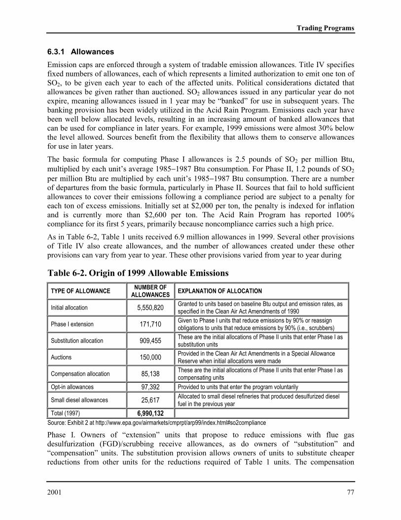
As in Table 6-2, Table 1 units received 6.9 million allowances in 1999. Several other provisionsof Title IV also create allowances, and the number of allowances created under these otherprovisions can vary from year to year. These other provisions varied from year to year during
Table 6-2. Origin of 1999 Allowable Emissions
TYPE OF ALLOWANCE NUMBER OFALLOWANCES EXPLANATION OF ALLOCATION
Initial allocation 5,550,820 Granted to units based on baseline Btu output and emission rates, asspecified in the Clean Air Act Amendments of 1990
Phase I extension 171,710 Given to Phase I units that reduce emissions by 90% or reassignobligations to units that reduce emissions by 90% (i.e., scrubbers)
Substitution allocation 909,455 These are the initial allocations of Phase II units that enter Phase I assubstitution units
Auctions 150,000 Provided in the Clean Air Act Amendments in a Special AllowanceReserve when initial allocations were made
Compensation allocation 85,138 These are the initial allocations of Phase II units that enter Phase I ascompensating units
Opt-in allowances 97,392 Provided to units that enter the program voluntarily
Small diesel allowances 25,617 Allocated to small diesel refineries that produced desulfurized dieselfuel in the previous year
Total (1997) 6,990,132Source: Exhibit 2 at http://www.epa.gov/airmarkets/cmprpt/arp99/index.html#so2compliance
Phase I. Owners of “extension” units that propose to reduce emissions with flue gasdesulfurization (FGD)/scrubbing receive allowances, as do owners of “substitution” and“compensation” units. The substitution provision allows owners of units to substitute cheaperreductions from other units for the reductions required of Table 1 units. The compensation

The U. S. Experience with Economic Incentives for Protecting the Environment
78 January
provision lets a utility reduce electricity generation of a Table 1 unit below its baseline level,provided the source of any compensating generation is designated. If the compensating unitemits SO2, EPA provides an allocation of allowances to that unit, so the compensating unit inessence becomes part of Table 1. Phase I initially included 263 units. An additional 125−182combustion units joined Phase I as compensation or substitution units (the totals varied by year).Several opt-in sources joined as well, raising the total of Phase I units to between 398 and 445units.
Beginning January 1, 1995, EPA could allocate up to 300,000 bonus allowances from itsConservation and Renewable Energy Reserve to utilities that undertake energy efficiency andrenewable energy measures. The full accounting of provisions for allocating 1999 allowances areidentified in Table 6-2 to illustrate the many sources of allowances.
In order to maintain the emissions cap, new sources receive no allowances. Instead, they mustbuy them from existing allowance holders or in EPA auctions. New sources are also required tosatisfy New Source Performance Standards.
In March 1995, EPA expanded the Acid Rain Program to include industrial facilities that burnfossil fuels.104 The rule establishes an “opt-in” program that allows industrial sources and othersources to participate in the existing SO2 program, which previously included only utilities.Industrial sources that participate in the program will have an allocation of allowances that theycan use for compliance or for selling or trading to other sources. These provisions allowingindustrial sources to opt-in have been little used, partially due to high transaction costs andlower-than-expected allowance prices.105 Ten units had joined the program as opt-in units by1999.
6.3.2 Monitoring and Compliance
Utilities whose units are included in Phase I and Phase II must install continuous emissionmonitoring (CEM) systems to verify compliance with emission limits, and they must filequarterly reports of their hourly emissions data with EPA. Initially, sources mailed these data toEPA on computer disks, but most sources now transmit the information over the Internet.Continuous emission monitoring systemsthe accepted industry standard for measuring SO2,NOx, and CO2provide an accurate accounting of emissions, assuring those buying and sellingallowances that the commodity they are trading is real and assuring EPA that emission limitshave been met.
CEMs for coal-fired electric power plants have an initial capital cost of just over $700,000, andannual operating costs of just under $50,000. On an annualized basis that spreads the capitalcosts over a capital recovery period, the cost of operating a CEM is approximately $125,000each year. This amount is equivalent to about $0.16 per kilowatt of installed capacity.106
The cost of monitoring with CEMS represents approximately 7% of the observed cost ofcompliance. More than 2,100 units are now required to have CEMS for Phase II of the program.This requirement helps ensure low transaction costs and confidence that each allowancerepresents one ton of SO2 emissions, regardless of where or when it is generated. Thatconfidence is an important underpinning of trading.
At the end of each quarter, EPA receives more than 1,700 reports containing hourly emissionsdata and heat input for affected units. More than 90% of this data is received electronically.
Trading Programs
2001 79
Using these data and the allowance record for each unit, EPA tracks compliance. CEMS providesome of the most accurate and complete data ever collected by EPA. In 1999, SO2 monitors onsources in the Acid Rain Program achieved a median relative accuracy of 3% and a medianavailability of 99.5%.
Under the authority of Title IV, EPA developed an allowance tracking system that serves as theofficial record of ownership and transfers. The system currently requires a paper form with thesignature of the seller, but it will allow transactions to be completed on the Internet by the end ofthis year. With just two staff members, EPA processes most allowance transactions within oneday of receipt.
6.3.3 Allowance Auction
In addition to private transactions in allowances, Title IV directed EPA to offer allowances at anannual auction, beginning in 1993. This auction offers the equivalent of roughly 2.8% of totalallowances. Private parties may also offer allowances at the auction. Each offer includes thequantity for sale and a minimum acceptable price. The auctions helped to provide a price signalto the allowance market in the early stages of the program and currently provide an additionalsource of allowances for utilities. The auctions have only involved allowances that can be used inthe current year and 6 and 7 years into the future. From now on, each auction will involvecurrent-year and 7-year allowances.
Before discussing the specifics of the auction, it is worth noting that it has largely served itspurpose now that (1) the market under the Acid Rain Program is flourishing and (2) the auctionactivity is dwarfed by the allowance exchanges occurring every day all over the country.Economists have criticized the mechanics of the auction, suggesting that it may also contribute tolower prices than otherwise would occur.107 The Act requires a discriminating price auction,which ranks bids from highest to lowest. EPA has interpreted this statement as requiring thateach seller receive the bid price of a specific buyer. The auction first awards allowances offeredby the seller with the lowest asking price to the bidder with the highest bid price. Incrementally,the allocation mechanism moves up the supply list and moves down the bid list until no bidder iswilling to offer what the remaining sellers are asking. The idea of having a discriminating priceauction came from staff members of the U.S. House of Representatives, who were convincedthat such an auction maximized revenue to sellers.108
This unusual auction mechanism may cause sellers to misrepresent and under-reveal their truecosts of emission control.109 By lowering the reservation price, a seller increases the probabilityof sale and the expected price, if buyers are offering different prices. Therefore, sellers would setlower reservation prices in such a discriminating price auction than in a single-price auction.Joskow (1998) concludes that EPA auctions became a sideshow to the much larger privatemarket, after just the first two auctions. (These two auctions provided useful indications early inthe process that allowance prices would be lower than first anticipated.)–The evidence from adetailed analysis of the auction records is that private sellers in the EPA auction have tended toset prices above market-clearing levels rather than too low, as initially hypothesized by Casonand others.
6.3.4 Transaction Costs
Many observers of the Acid Rain Program have noted the low transaction costs of the allowancemarket. The allowance market operates on a very narrow bid—to-ask spread. Recently, this

The U. S. Experience with Economic Incentives for Protecting the Environment
80 January
spread has been less than $2 per ton, or about 1% of allowance prices. Most allowance transfersare processed within 24 hours of receipt, as program requirements eliminate the need for reviewof submissions beyond electronic verification that the allowances being transferred are indeed inthe seller’s account. In addition, program design eliminates the need for source-specific emissionlimits or reviews of compliance strategies, causing the costs of oversight to drop dramatically.
During the 5 years following the Clean Air Act Amendments, EPA spent $44 million toimplement the Acid Rain Program and allocated an additional $18.9 million to state and localgovernments to implement the program. These costs may be compared with the $1.09 billion thatEPA spent to implement the Clean Air Act in the same period and the $833 million EPAdistributed to state and local governments for this purpose.110
6.3.5 Results
From 1995 through 1999, the Acid Rain Program has exceeded expectations, with firmsexceeding the reduction target at less than one-half the forecast cost. These results follow fromthe very flexible structure of the program, one key component of which was the tradingprovision.111
While there was considerable trading activity from the start, little of that activity initially wasbetween economically distinct entities. (See Figure 6-1.) In searching for explanations for therelatively low level of tradingbetween economically distinctentities (labeled “external” inFigure 6-1), analysts have citedrelatively high transaction costsat first, the behavior of publicutility commissions, andlegislation in some states thatpromoted the use of locallyproduced coal.
Emissions data compiled byEPA show at least 9,300transfers involving 81.5 millionallowances through the end of1999. About 62% of theallowances or 50.4 million tonswere transferred withinorganizations, and 38% or 31million tons were transferredbetween organizations. Another40 million tons reflectmovements of allowances from EPA to the market through auctions, Phase I extensionallowances, substitution allowances, and other mechanisms. SO2 emissions control is ahead ofschedule. The excess emissions reductionsunused allowancesin Phase I are being banked byutilities for use during Phase II, when the performance standard tightens significantly.
Figure 6-1. Internal and External Trading
0
2
4
6
8
10
12
14
16
1994 1995 1996 1997 1998 1999
INTERNAL EXTERNAL
Source: Exhibit 6 athttp://www.epa.gov/airmarkets/cmprpt/arp99/index.html#so2compliance

Trading Programs
2001 81
The price of allowances has been far below initial forecasts, an issue that has attractedconsiderable attention. Prior to passage of the Clean Air Act Amendments of 1990, industryestimates of abatement costs were $1,000 per ton, and EPA forecast allowance prices were in the$750-per-ton range. As an ultimate backstop for compliance, Congress authorized directallowance sales by EPA at a price of $1,500 per ton. The direct sale provisions were eliminatedseveral years ago when it became clear that allowance prices were far lower than anticipated, andthe direct sale option would not be utilized.
Some early allowance transactions occurred at prices as high as $300 per ton in 1992. By 1993,the price had fallen to a range of $150 per ton to $200 per ton. Allowance pricesfrom EPAauctions, transactions through the Emissions Exchange, and through brokersgradually fell to alow of $66 per ton through mid-1995 and, in general, remained below $120 per ton through1997. (See Figure 6-2.) In 1998, allowance prices began to increase and exceeded $200 per tonby early 1999, peaking at $217 per tonin March. Prices then declined to about$130 ton by March 2000.112
Lower-than-forecast allowance priceshave several explanations. Prices forvirtually every form of compliance arewell below anticipated levels. The priceof low-sulfur western coal delivered toMid-West and Eastern markets hasdeclined due to productivityimprovements in extraction andtransport, and deregulation of rail rates.Engineers have found ways to blendlow-sulfur Western coal with high-sulfur Eastern coal to meet emissionlimits in boilers that had been designedto burn high-sulfur coal. In addition, innovations in the scrubber market have cut the cost ofscrubbing by approximately one-half. Many utilities committed themselves to scrubbers andother relatively expensive control measures, based on early engineering cost studies. If utilitieshad anticipated SO2 control costs better, fewer scrubbers would have been placed in service. Theconsequence of greater-than- expected compliance is downward pressure on allowance prices inPhase I.
Analysts debate the role that allowance trading plays in stimulating cost effectiveness in SO2
control from power plants. There is no doubt that SO2 control has experienced tremendoustechnological and productivity improvement over a very short period of time, leading toapproximately 50% lower costs for controlling emissions than had been anticipated. The issue isthe extent to which allowance trading should be credited with these gains. Burtraw (1995)reached two conclusions. First, it is the flexible, performance-based design of the program thathas stimulated the development of low-cost compliance measures seen in Phase I. Second, withinthat framework, allowance trading played an important, positive role. Ellerman (2000) attributesall of the cost savings to trading provisions. The difference in the two points of view isconsiderable. Ellerman gives credit to emissions trading for a dramatic fall in the cost ofscrubbing emissions and for the growing use of low-sulfur Western coal. In contrast, Burtraw
Figure 6-2. Acid Rain Allowance Prices
$0
$50
$100
$150
$200
$250
Aug
-94
Feb
-95
Aug
-95
Feb
-96
Aug
-96
Feb
-97
Aug
-97
Feb
-98
Aug
-98
Feb
-99
Aug
-99
Feb
-00
Source: Exhibit 5 athttp://www.epa.gov/airmarkets/cmprpt/arp99/index.html#so2compliance

The U. S. Experience with Economic Incentives for Protecting the Environment
82 January
credits performance standards and flexible program design, not emissions trading directly, formuch of the cost savings.
Phase II of the Acid Rain Program is likely to see much greater reliance on allowance trading.Phase II will involve 700 additional sources, many of which are likely to select scrubbing as theirmethod of compliance. More scrubbing should result in greater variation in the marginal costs ofcontrol across sources. Consequently, there should be greater incentives to trade allowances toachieve compliance in Phase II.
A 1995 EPA assessment of the Acid Rain Program put the costs at $1.2 billion annually in PhaseI and $2.2 billion annually in Phase II.113 The same EPA report estimated the mean value ofannual health benefits at $10.6 billion in Phase I and $40 billion in Phase II. These healthbenefits are limited to benefits from reduced sulfates; total health benefits would be even higher.Interestingly, health benefits were not a major concern in the legislative decision to control acidrain, yet they now appear to be the dominant benefit component, dwarfing earlier estimates ofenvironmental effects. Recall that early estimates of the costs of controlling acid rain put thecosts at $4.5 billion to $6 billion annually with a traditional regulatory approach and benefits at$1 billion to $2 billion. An independent assessment reached a similar conclusion: Benefits willbe much greater than costs.114 More recent studies have estimated Phase II costs at $1.0 billion(Carlson et al., 2000) and $1.4 billion (Ellerman, 2000, p. 282).
To estimate the savings attributable to tradable allowances, Carlson et al. (2000) estimatedmarginal abatement cost functions for thermal power plants that were affected by Title IV. Forplants that use low-sulfur coal as a means of compliance, they found that the main sources ofcost reductions are technological improvements and the fall in low-sulfur coal prices, notallowance trading. Over the long run, the authors estimate that allowance trading could result insavings of $700 million to $800 million per year, relative to an “enlightened” regulatoryapproach with a uniform emission standard.
6.4 NOx Regional Ozone Programs
The federal SO2 control program shows that acid rain poses a number of difficult problems forpolicy makers, regulators, environmentalists, and industry. Experiences with the SO2 programwere instrumental in designing and implementing the recent NOx control program.
Along with SO2, NOx contributes to the acid rain problem nationwide. NOx also contributes toground-level ozone and fine particulate problems in the East and in certain densely populatedareas elsewhere. With respect to acid rain, both SO2 and NOx have cumulative and long-rangeimpacts on the environment. With respect to ground-level ozone and fine particulate matter, theprimary concern is ambient concentrations over short periods of time during the summer months.
NOx trading is designed to account for these complex time and space dimensions in the need tocontrol NOx. Electric power generation peaks in summer months in the Northeast to meet airconditioning demands. Periods of peak power production are periods of peak NOx emissions andtend to be periods of time when ambient ground-level ozone concentrations are most likely toexceed federal standards.
Trading Programs
2001 83
6.4.1 OTC NOx Budget Program
In the 1990 Clean Air Act Amendments, Congress established the Ozone Transport Commission(OTC), a working group consisting of 12 Northeast states and the District of Columbia. OTC’smandate was to develop plans to meet national ambient air quality goals for ozone in the EasternUnited States. With the help of EPA, the OTC developed a NOx Budget Program to addressregional ozone problems. Critical program elements, such as monitoring and reportingprovisions, compliance determination, and penalties, were required to be uniform across states. A1994 memorandum of understanding with EPA was signed by all of the OTC states, exceptVirginia. It put in place a NOx cap-and-trade system within the OTC states. The intent of theagreement is to institute a cooperative effort to solve a common problem.
The agreement caps NOx emissions at 219,000 tons during the May through Septembercompliance period for the years 1999−2000 and at 143,000 tons starting in 2003. Both amountsare less than one-half the 1990 baseline of 490,000 tons. The cap affects 465 sources of NOx inthe participating OTC states, including utilities, industrial plants, and independent powerproducers.
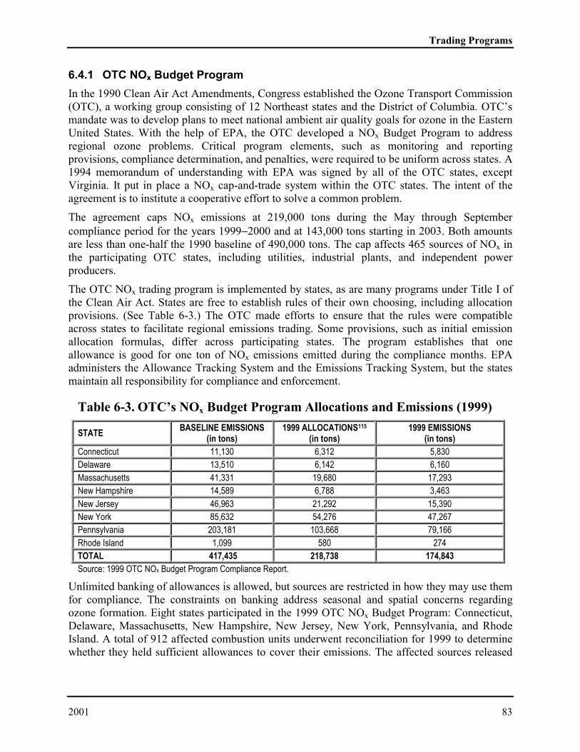
The OTC NOx trading program is implemented by states, as are many programs under Title I ofthe Clean Air Act. States are free to establish rules of their own choosing, including allocationprovisions. (See Table 6-3.) The OTC made efforts to ensure that the rules were compatibleacross states to facilitate regional emissions trading. Some provisions, such as initial emissionallocation formulas, differ across participating states. The program establishes that oneallowance is good for one ton of NOx emissions emitted during the compliance months. EPAadministers the Allowance Tracking System and the Emissions Tracking System, but the statesmaintain all responsibility for compliance and enforcement.
Table 6-3. OTC’s NOx Budget Program Allocations and Emissions (1999)
STATE BASELINE EMISSIONS(in tons)
1999 ALLOCATIONS115
(in tons)1999 EMISSIONS
(in tons)Connecticut 11,130 6,312 5,830Delaware 13,510 6,142 6,160Massachusetts 41,331 19,680 17,293New Hampshire 14,589 6,788 3,463New Jersey 46,963 21,292 15,390New York 85,632 54,276 47,267Pennsylvania 203,181 103,668 79,166Rhode Island 1,099 580 274TOTAL 417,435 218,738 174,843Source: 1999 OTC NOx Budget Program Compliance Report.
Unlimited banking of allowances is allowed, but sources are restricted in how they may use themfor compliance. The constraints on banking address seasonal and spatial concerns regardingozone formation. Eight states participated in the 1999 OTC NOx Budget Program: Connecticut,Delaware, Massachusetts, New Hampshire, New Jersey, New York, Pennsylvania, and RhodeIsland. A total of 912 affected combustion units underwent reconciliation for 1999 to determinewhether they held sufficient allowances to cover their emissions. The affected sources released

The U. S. Experience with Economic Incentives for Protecting the Environment
84 January
emissions at a level nearly 20% below their allocations for 1999, banking the remainder forfuture use when emission limits will be stricter.116
The market is showing signs of maturing. Trades for future year allowances have higher prices,which reflect the anticipated difficulty of meeting a shrinking cap on emissions. Similar pricespreads also exist in the SO2 allowance market.
6.4.2 NOx Budget Trading Program
EPA promulgated the call for State Implementation Plans (SIPs) on NOx, (the NOx SIP call)pursuant to the requirements of Section 110 of the Clean Air Act (CAA). Section 110 requires aSIP to contain adequate provisions that prohibit any source or type of source or other types ofemissions within a state from emitting any air pollutants in amounts that will contributesignificantly to non-attainment in, or interfere with maintenance of attainment of a standard by,any other State with respect to any National Ambient Air Quality Standard (NAAQS). Section110 authorizes EPA to find that a SIP is substantially inadequate to meet any CAA requirementwhen appropriate, and, based on such finding, to then require the state to submit a SIP revisionwithin a specified time to correct such inadequacies.
The final rule required 22 states and the District of Columbia to submit State ImplementationPlans that address the regional transport of ground-level ozone. The rule will reduce totalsummertime emissions of nitrogen oxides by about 28% (1.2 million tons) in the affected statesand the District of Columbia. The final rule includes a model NOx Budget Trading Program thatwill allow states to achieve over 90% of the required emissions reductions from large electricgenerating sources and large industrial boilers in a highly cost-effective way.
The NOx SIP call was challenged by representatives of both industry and affected states. In May1999, the U.S. Court of Appeals for the District of Columbia Circuit stayed the submittaldeadline of the NOx SIP call indefinitely. In November 1999, oral arguments were heard and, inMarch 2000, the Appeals Court ruled in favor of EPA on all major issues, remanding to EPAonly a few minor issues.
As a result of its ruling, three states were no longer required to comply with the NOx SIP call(Wisconsin, Georgia, and Missouri), and EPA was required to take further notice and commenton a portion of its electric generation unit (EGU) definition. Sources in several states will besubject to this action: Alabama, Connecticut, District of Columbia, Delaware, Illinois, Indiana,Kentucky, Massachusetts, Maryland, Michigan, North Carolina, New Jersey, New York, Ohio,Pennsylvania, Rhode Island, South Carolina, Tennessee, Virginia, and West Virginia. In June2000, the Appeals Court lifted the stay and ruled that affected states must submit SIPs to EPA bythe end of October 2000. In August 2000, the court made another ruling. This ruling moved thecompliance date to submit SIPs to May 31, 2004, from its original date of May 1, 2003. As ofSeptember 2000, EPA had not yet decided whether to appeal this ruling.
The petitioners have asked the Supreme Court to review the Appeals Court’s decision. As ofAugust 2000, the Supreme Court had not decided to hear the case.
Section 126 of the Clean Air Act allows states that are adversely affected by interstate transportof pollution to petition EPA to set pollution limits on specific sources of pollution in other states.In a December 17, 1999 rule, EPA granted petitions filed by Connecticut, Massachusetts, NewYork, and Pennsylvania that sought to reduce ozone in these states through the control of NOx

Trading Programs
2001 85
emissions from other states.117 These states had petitioned that they could not attain the federal 1-hour ozone standard because of the interstate transport of ozone and its precursors.
Under its Section 126 authority, EPA published a final rule that affects 392 electric utilities andindustrial boilers with rated output greater than 25 megawatts or a maximum heat input capacitygreater than 250 MMBtu/hr. The Federal NOx Budget Trading Program establishes emissionlimits for affected sources in the form of tradable NOx allowances. One allowance authorizes theemission of one ton of NOx. Sources in the program are located in Delaware, the District ofColumbia, Indiana, Kentucky, Maryland, Michigan, North Carolina, New Jersey, New York,Ohio, Pennsylvania, Virginia, and West Virginia. Collectively, they must reduce NOx emissionsby nearly 530,000 tons per year by 2007 from levels had been allowed that year.
Both the NOx SIP call and the Section 126 action require sources to reduce emissions of NOx.However, the SIP call allows states the flexibility to choose how reductions will be made; underthe 126 action, EPA directly regulates sources. Furthermore, the SIP call covers a largergeographic area. EPA is continuing to work with the states to determine how to integrate thesetwo programs.
6.5 Chlorofluorocarbon (CFC) Production Allowance Trading
The Montreal Protocol on Substances that Deplete the Ozone Layer called for a cap onchlorofluorocarbon (CFC) and halon consumption at 1986 levels, with reductions in the capscheduled for 1993 and 1998. At a second meeting in 1990, the parties to the Montreal Protocolagreed to a full phaseout of the already-regulated CFCs and halons, as well as a phaseout of“other CFCs,” by 2000.118
The Montreal Protocol defined consumption as production plus imports, minus exports.Consequently, in implementing the agreement, EPA distributed allowances to companies thatproduced or imported CFCs and halons. Based on 1986 market shares, EPA distributedallowances to 5 CFC producers, 3 halon producers, 14 CFC importers, and 6 halon importers.
The marketable permit system for producers and importers resulted in a number of savingsrelative to a program that directly controlled end uses. EPA needed just 4 staffers to oversee theprogram, rather than the 33 staffers and $23 million in administrative costs it anticipated wouldbe required to regulate end uses. Industry estimated that a traditional regulatory approach to enduses would cost more than $300 million for recordkeeping and reporting, versus only $2.4million for the allowance trading approach.
Title VI of the Clean Air Act Amendments of 1990 modified the trading system to allowproducers and importers to trade allowances within groups of regulated chemicals that weresegregated by their ozone-depleting potential. As an example, EPA assigned producers andimporters allowances for five types of CFCs (CFC-11, CFC-12, CFC-113, CFC-114, and CFC-115). Producers and importers could trade allowances within this group. For example, 14 millionkilograms of CFC-11 and CFC-113 were traded for CFC-12 in 1992 as air conditioner makersand foam producers reduced their use of these substances. At the same time, CFC-12 usersmaintained their demand. By 1994, the quantity of CFC-11 and CFC-113 swapped for CFC-12grew to 26 million kilograms. EPA rules implementing Title VI specify that, each time aproduction allowance is traded, 1% of the allocation is “retired” to assure further improvement inthe environment.

The U. S. Experience with Economic Incentives for Protecting the Environment
86 January
Congress coupled the marketable allowance trading system with excise taxes on CFCproduction, which are discussed in Chapter 4, Pollution Charges, Fees, and Taxes. The rationalefor the excise taxes was that the restrictions on the quantity of CFCs and halons could be soldwould lead to rapidly escalating prices. The excise taxes were designed to capture “windfallprofits.” In contrast, the allowance trading system was designed to assure that the production andimport of the CFCs was cost-effective. The excise tax has the effect of making CFCs much moreexpensive in the United States than they are in developing countries where production is stillallowed. Smuggling of these chemicals has become a serious problem.
6.6 Lead Credit Trading
As early as the 1920s, tetra-ethyl lead was added to gasoline by refiners to increase octane levelsand reduce premature combustion in engines, which allowed more powerful engines to be built.Lead additives in gasoline were the least expensive of several ways of raising octane levels. Theadditives also prevented premature recession of soft-valve seats, a feature of most automobileengines that were manufactured prior to 1975 (but not after).
By the 1970s, virtually all gasoline contained lead at an average of almost 2.4 grams per gallon.EPA acted to curtail lead use in gasoline for two reasons. One, by 1975 new production vehicleswere equipped with exhaust system catalysts, so these vehicles could meet the tailpipe emissionstandards for hydrocarbons, carbon monoxide, and nitrogen oxides that were mandated by the1970 Clean Air Act. Unleaded fuel was required for vehicles manufactured after model year1975, since exhaust system catalysts would be fouled and not function properly if vehicles wererun on leaded gasoline. As catalyst-equipped vehicles began to dominate the fleet, sales ofunleaded gasoline reached about 80% of all gasoline sales by the mid-1980s.
Two, concerns about the role of airborne lead in adult hypertension and cognitive developmentin children motivated EPA to limit the overall use of lead in gasoline. EPA required that theaverage lead content of all gasoline sold be reduced from 1.7 grams per gallon after January 1,1975, to 0.5 grams per gallon by January 1, 1979. Initially, these limits were applicable asquarterly averages for the production of individual refineries, implicitly allowing trading acrossbatches of gasoline at individual refineries. Later, EPA broadened definition of averaging toallow refiners who owned more than one refinery to average or “trade” among refineries tosatisfy their lead limits each quarter.
During the late 1970s, the demand for unleaded gasoline grew steadily as more catalyst-equippedvehicles were sold. By the early 1980s, the market share of leaded gasoline had shrunk to thepoint that EPA’s limits on the average lead content of all gasoline ceased to have an impact onthe lead content in leaded gasoline. Meanwhile, evidence on the magnitude and severity of thehealth effects attributable to lead mounted.
EPA acted to curtail sharply the remaining use of lead in gasoline, initially setting a limit of anaverage level of 1.1 gm/gal beginning on November 1, 1982. EPA lowered the average to 0.5gm/gal by July 1, 1985, and then to 0.1 gm/gal by January 1, 1986. To facilitate the phasedown,EPA allowed two forms of trading: inter-refinery averaging during each quarter and banking forfuture use or sale.
Inter-refinery averaging, which operated from November 1, 1982, to December 31, 1985,allowed refineries to “constructively allocate” lead. To take an example, suppose refiner Aproduced 200 million gallons of gasoline in the first quarter of 1983 with an average lead content

Trading Programs
2001 87
of 1.4 gm/gal. Refiner A could buy 60 million grams of lead credits from Refiner B, whoproduced an equal quantity of gasoline with lead content of 0.8 gm/gal. In 1985, EPA permittedrefiners to bank credits for use until the end of 1987, which in effect extended the life of leadcredits to that date.
Lead credits were created by refiners, importers, and ethanol blenders (who reduced the leadcontent of gasoline by adding ethanol). For example, when the average lead content was limitedto 1.0 gm/gal, a refiner producing 1 million gallons of gasoline with an average lead content 0.5gm/gal would earn 500,000 lead credits. EPA enforcement relied on reporting requirements andthe random testing of gasoline samples. Reporting rules were simple. Each refiner or importerwas obligated to provide the names of entities with whom it traded, the volumes for each trade,and the physical transfer of lead additives. The data allowed EPA to compare reported leadadditive purchases and sales for each transaction to assure compliance. Discrepancies in reportedfigures could trigger investigations and enforcement actions. Well over 99% of all transactionswere reported accurately; however, several dozen fraudulent transactions occurred.119 In onequarter alone, the now-defunct Good Hope refinery in Louisiana accounted for over one-half ofall reported lead credits sold during one quarter. Subsequent investigation uncovered the fraud.
Judged by market activity, lead credit trading was quite successful. Lead credit trading as apercentage of lead use rose above 40% by 1987. Some 20% of refineries participated in tradingearly in the program; by the end of the program, 60% participated.120 Early in the program, 60%of refineries participated in banking, rising to 90% by the end. Trading allowed the EPA to phaseout the use of lead in gasoline much more rapidly than otherwise would have been feasible.Given that refiners faced very different opportunities for reducing the lead content of gasoline, arapid phase-down without trading would have rewarded refiners collectively, since the marketprice of gasoline would have been determined by the high-cost producers.
During the period of time when lead credits were traded, the price increased from about 3/4cent/gm to 4 cents/gm.121 Nearly one-half of all lead traded was between refineries owned by thesame firm.122 With external transactions, refiners revealed a preference to deal with normaltrading partners, even though they could obtain a better price elsewhere. This preferenceindicates that trading did not produce the least cost outcomes, even though there was an activemarket in lead credits. In part, this result occurred because internal trades have lower transactionand information costs than inter-refinery trades. However, it also reflects strong preferences inthe industry to avoid revealing potentially valuable information to competitors.
EPA estimated that the banking provisions alone would involve 9.1 billion grams of lead creditsand save refiners $226 million. Subsequently, the amount of lead banked was placed at just over10 billion grams. Lead credit trading may be viewed in retrospect as a considerable success. Theuse of lead in leaded gasoline was sharply reduced over a short period of time, without spikes inthe price of gasoline that otherwise might have occurred. The market in lead credits was quiteactive, although, as noted in the previous paragraph, refiners did not maximize their gains fromtrade. In addition, some small refiners and ethanol blenders nonetheless sold many more creditsthan they had earned, despite seemingly foolproof procedures for catching fraudulent trades.
6.7 Gasoline Constituents
Title II of the Clean Air Act Amendments of 1990 imposes substantially tightened mobile sourceemission standards by requiring automobile manufacturers to reduce tailpipe emissions and by

The U. S. Experience with Economic Incentives for Protecting the Environment
88 January
requiring refiners to develop reformulated fuels. The Amendments require reductions in tailpipeemissions of 35% for hydrocarbons and 60% for NOx, starting with 40% of the vehicles sold in1994 and increasing to all vehicles sold in 1996. Light-duty trucks are subject to similarrequirements. EPA is required to impose further reductions of 50% below these standards by2003 if it finds such reductions are necessary, technologically feasible, and cost-effective. EPArecently issued Tier 2 gasoline sulfur standards that implement this further reduction.
Title II requires that states having CO non-attainment areas with design values of 9.5 parts permillion (ppm) or higher must implement a program to supply oxygenated fuels to motorists inwinter months. (The term “design values” is defined as the second highest ambient readingmeasured over the most recent two years.) Gasoline sold in the 41 cities affected by thisrequirement must have an oxygen content of 2.7% starting in 1992. To meet the percent oxygenrequirement, states are “strongly encouraged” to create a program for marketable oxygen creditsto provide flexibility to gasoline suppliers.
In October 1992, EPA issued guidance for trading programs in oxygenates under the wintertimeoxygenated gasoline program; however, participation is optional for the affected states.123 Inareas where trading is permitted, credits in oxygenates can be exchanged between parties that thestate has designated as responsible for satisfying fuel requirements, also known as the ControlArea Responsible Party or CAR. Normally the CAR is the party who owns gasoline at aterminal. The CAR receives data on the volume and oxygen content of all gasoline shipped to theterminal and assures that the average oxygen content is 2.7% by weight. Where trading isallowed, the CAR would be free to sell excess oxygenate credits to other CARs or buy oxygenatecredits from a CAR to meet the 2.7% requirement. While trading in oxygenates theoreticallyoffers a cost-effective means of meeting wintertime oxygenate requirements, in fact, the tradingprograms have been moribund. Only the Pennsylvania part of the Philadelphia ozone non-attainment area (which also includes parts of New Jersey) adopted trading rules. Within that area,no trades have been reported. Other areas have declined to allow trading, citing the costs ofmonitoring such a program as prohibitive.
Title II also requires that the 9 worst ozone non-attainment areas offer reformulated gasolineduring the summer months. It also specifies several performance characteristics for reformulatedgasoline as well as certain fuel properties, including a minimum oxygen content of 2% by weightbeginning in 1995. Under so-called “opt in” provisions, an additional 31 areas applied to EPA, sothey could participate in the reformulated gasoline program.
Title II requires that EPA establish trading systems for three constituents of reformulated fuels:oxygen, aromatics, and benzene. Under a trading system, refiners could meet reformulatedcontent requirements by producing gasoline that met the specifications or by trading credits inthese constituents with other refiners, so collectively the standards were satisfied. EPA’s rulesfor reformulated gasoline set up an averaging-and-trading system as well as an averaging-and-trading system for meeting EPA’s performance standards for VOCs and toxic air chemicals.
There has been considerable trading and averaging of reformulated gasoline requirements,mainly from the Midwest to the East Coast. That trading has led to some regional failures tomeet oxygenate retail averages, and it has resulted in a tightening of the oxygenate standards forreformulated gasoline.

Trading Programs
2001 89
6.8 Tier 2 Emission Standards
On February 10, 2000, EPA promulgated new standards for tailpipe emissions of NOx frompassenger cars and light-duty trucks and for the sulfur content of gasoline.124 The tailpipeemission action was taken under EPA’s authority to set tailpipe emission standards for newvehicles (Section 202 of the Clean Air Act). The fuel standard action was based on EPA’sdetermination that motor vehicle fuels contribute to air pollution and adversely affect theperformance of emission control systems (an authority under Section 211 (c)(1) of the Clean AirAct).
Manufacturers will be able to average their Tier 2 vehicles to comply with the corporate averageNOx tailpipe standard of 0.07 grams per mile (gpm), which is more than a 75% reduction fromthe current 0.30 gpm. standard.125 When a manufacturer’s corporate average NOx emissions fallbelow the standard, it will earn credits that may be banked for later use or sold to anothermanufacturer. These credits will be very similar to those currently in place for non-methaneorganic gas (NMOG) emissions under California and the federal National Low Emission Vehicle(NLEV) regulations. The NOx credits will have unlimited life. Manufacturers would be permittedto run a credit deficit for 1 year and carry forward that deficit. If the manufacturer has a creditdeficit in the second year, the manufacturer would be subject to an enforcement action.
Refiners and gasoline importers must satisfy a corporate average gasoline standard of 120 ppmand a cap of 300 ppm sulfur beginning in 2004. In 2005, this corporate average standard drops to90 ppm sulfur, with the cap remaining at 300 ppm. The format of the program changes in 2006from a corporate average to a per-refinery requirement. At that time, the cap will be 80 ppmsulfur, and most refiners will have to produce gasoline that averages no more than 30 ppm sulfur.Refiners who produce gasoline with a corporate average sulfur content lower than the standardwill be allowed to bank credits for future use or for sale to other refiners that are unable to meetthe standard. Credits produced under the phase-in years have a limited life. Those creditsproduced beginning in 2006 have an unlimited life. The program runs until 2010. However,refiners will be able to carry forward a deficit for 1 additional year, providing that the average isbelow 80 ppm sulfur.
The standards concern hydrocarbon emissions, which was termed “NMOG” in the rulemaking.Manufacturers would have to satisfy a corporate average standard, but they could meet thisstandard through the trading of credits earned by manufacturers that exceeded the corporateaverage standard. Banking also would be allowed. Banked credits, however, would be subject todiscounting over time.
6.9 Heavy-Duty Truck Engine Emission Averaging
Title II of the Clean Air Act Amendments of 1990 authorizes EPA to set standards for particulatematter, NOx, and other emissions from heavy-duty truck engines. The standards must representthe maximum degree of reductions achievable, taking cost and other factors into consideration.EPA has interpreted this provision to authorize the use of averaging, banking, and trading as partof the process of realizing the maximum degree of reductions achievable.
Under this program, there has been a great deal of averaging and banking but only one tradebetween firms, a 1996 exchange of rights to 5 tons of particulate matter from Navistar to DetroitDiesel. The averaging of emissions facilitates compliance, since not every class of engines has to
The U. S. Experience with Economic Incentives for Protecting the Environment
90 January
meet the 75% reduction standard. How much engine manufacturers actually save is unknown.However, a recent paper examined a similar type of engine performance averaging program thatwas proposed in California for light-duty trucks. It concluded that the cost savings of theprogram were likely to be modest.126
6.10 Corporate Average Fuel Economy (CAFE) Standards
The Energy Policy and Conservation Act of 1975 established corporate average fuel economy(CAFE) standards for all manufacturers that sell vehicles in the United States. The standardswere first imposed in 1978 and are now 27.5 miles per gallon (mpg) for production passengercars and 20.7 mpg for production light-duty vehicles. (Light-duty vehicles include sport utilityvehicles, minivans, and pickup trucks with gross vehicle weight ratings less than 8500 pounds.)
Corporate average fuel economy and compliance with the CAFE standard is determined as theharmonic mean of the fuel economy of automobiles produced by each manufacturer.127
Harmonic average fuel economy is more difficult to achieve than is simple averaging. Forexample, to achieve a CAFE standard of 27.5 mpg, two 35-mpg vehicles must be sold for every20-mpg vehicle sold. The penalty for failing to meet the CAFE standard is $5.50 per automobilefor every 0.1-mpg shortfall. Carry back and carry forward provisions akin to banking do exist,and they allow shortfalls in one year to be met with credits from another year.
CAFE standards have been the primary national policy instrument for improving personalvehicle fuel economy and for reducing gasoline and oil consumption in the transportation sector.From the late 1970s through the mid-1980s, CAFE standardsworking in concert with highergasoline prices through most of that periodnearly doubled the average fuel economy of newpersonal vehicles. Throughout the 1990s, with oil and gasoline prices recording historic lows onan inflation-adjusted basis, CAFE standards provided a floor for automotive fuel economy. Fueleconomy was higher than it would have been absent the standards. Therefore, compliance withthese standards reduced gasoline consumption.
Since fuel economy is inversely proportional to carbon dioxide emissions, the primarygreenhouse gas from motor vehicles, CAFE has yielded reductions in carbon dioxide emissionsand overall greenhouse gas emissions. (Fuel economy is largely unrelated to emissions of criteriapollutants such as particulate matter, CO, and NOx). In this regard, CAFE can be viewed as anintra-firm trading system to meet a de facto standard to reduce the carbon dioxide emissionsfrom personal vehicles.
As a policy instrument, CAFE has both advantages and disadvantages. Some of CAFE’sadvantages follow.
• CAFE is in place, it has proven to be a workable program, and lessons have been learnedabout how it could be improved.
• CAFE has yielded significant reductions in gasoline consumption and carbon dioxideemissions, which would not have been the case without these standards.
• The general public strongly supports CAFE relative to other alternatives to increase fueleconomy and reduce carbon dioxide emissions, such as higher gasoline taxes.
• CAFE includes many market elements, such as

Trading Programs
2001 91
• sales-weighted averaging (as opposed to a floor that every vehicle must meet),
• a 7-year rolling average for compliance (and credits can be carried back or forward for 3years), and
• the option of paying monetary fines in lieu of meeting the standard, a choice that is left tothe discretion of the manufacturer. (Several non-U.S. firms pay these fines. All U.S.automakers have chosen to meet CAFE standards in the past.)
Like any policy instrument, CAFE also has disadvantages. Some of them follow.
• CAFE is inconsistent with low fuel prices. That is, when gasoline prices are relativelylow, there is less demand for high-fuel economy cars, and manufacturers must sell higherfuel economy than the market demands.128
• CAFE does nothing to reduce vehicle miles traveled (VMT). (Some analysts argue thatCAFE increases VMT and emissions by lowering the cost of driving, i.e., raising the fueleconomy of vehicles means, in theory, that less gasoline is needed to travel a certainnumber of miles. Other analysts assert that these effects are negligible.)
• CAFE does have a cost, either in terms of the higher prices of vehicles or the tradeoffsthat must be made with other vehicle attributes such as utility, weight, or acceleration.
• CAFE is strongly opposed by automakers, whose objections include higher vehicle costand the potential reduction in safety for passengers in these lighter weight vehicles.
Alternatives to CAFE standards would include higher gasoline taxes and “feebates,” whichwould assess fees to the sale of vehicles with low-fuel economy and rebates for the purchase ofhigh-fuel economy vehicles. Like CAFE, each of these options has advantages anddisadvantages. The relative merits of these options relative to CAFE are debated, as is themagnitude required for such policies to provide the same benefits as CAFE.
6.11 Hazardous Air Pollutant (HAP) Early Reduction
In December 1992, EPA issued final rules for the early reduction of hazardous air pollutants.129
If a facility qualifies for inclusion in the program by reducing hazardous air pollutants by90%95% in the case of hazardous particulate emissionsprior to EPA proposing maximumavailable control technology (MACT) regulations on the source category, the facility may defercompliance with the new MACT for as long as 6 years. Because participation in the program isvoluntary, a source must anticipate cost savings, or it would not have an incentive to participate.Once a source is accepted into the program, it becomes legally obligated to meet the 90% (or95%) reduction in emissions. Trading exists intertemporally across time in that sources exchangetheir early reductions for their later reductions. (The example in the next paragraph illustrateshow this program works.)
EPA has shown that such a program can benefit the environment. Assume a source emits 100tons per year. Under the early reduction program, it would emit 10 tons per year. Further assumethat MACT would have the source reduce emissions to 2 tons per year in year 5 and thereafter.The source has reduced emissions by 360 tons in years 1 through—4 in exchange for 48 tons ofemissions in years 5 through10. Total emissions are reduced by 312 tons. Table 6-4 illustratesthe time profile of emissions.

The U. S. Experience with Economic Incentives for Protecting the Environment
92 January
By mid-1993, over 60 chemical plants had asked to participate in the program, so they couldavoid the synthetic organic chemical MACT standard for 6 years. Other types of facilities alsohad applied to join the program.130
Table 6-4. Benefits of Achieving Early Emission Reductions
YEAR MACT EMISSIONS (in tons) EARLY REDUCTION EMISSIONS (in tons)1 100 102 100 103 100 104 100 105 2 106 2 107 2 108 2 109 2 10
10 2 10TOTAL 412 100
Source: 57 FR 61970
6.11.1 The Petroleum Industry NESHAP
EPA’s National Emission Standard for Hazardous Air Pollutants (NESHAP) rule, promulgatedon August 18, 1995, establishes Maximum Available Control Technology (MACT) requirementsfor process vents, storage vessels, wastewater streams, and equipment leaks at refineries. Therule specifically includes marine tank vessel-loading activities and gasoline loading racks.
The rule excludes distillation units at pipeline pumping stations and certain process vents thatEPA determined would be subject to future NESHAP rules: catalyst regeneration on crackingunits, vents on sulfur recovery units, and vents on catalytic reforming units.
On September 19, 1995, EPA issued a final NESHAP rule for marine vessel tank-loadingoperations. The rule affects new and existing marine bulk loading and unloading facilities thatemit 10 tons or more of a single hazardous air pollutant (HAP) or 25 tons of any aggregateHAPs. Affected facilities must install a vapor collection system to collect volatile organiccompounds (VOCs) that are displaced from marine tank vessels during loading. The vaporrecovery system must achieve a 95% reduction in emissions, 98% if combustion is used.
Both of these NESHAP rules permit the use of emissions averaging among marine tank vessel-loading operations, bulk gasoline terminal or pipeline breakout station storage vessels and bulkgasoline loading racks, and petroleum refineries. Emissions averaging gives the owner theopportunity to find the most cost-effective control strategies for a particular situation. The ownermay over-control at some emission points and under-control at others to achieve the overall levelof emissions control that is required.
6.11.2 Hazardous Organic Chemical NESHAP
The Hazardous Organic Chemical NESHAP (or “HON”) affects more than 400 facilities of theSynthetic Organic Chemical Manufacturing Industry (SOCMI). The final rule requires sources tolimit emissions of organic hazardous air pollutants (HAPs) and to apply “reference control” or

Trading Programs
2001 93
equivalent maximum available control technology (MACT). In recognition of the high costs ofsome MACT controls in this industry, the rule allows emissions averaging. Under this alternativemethod of compliance, sources engaging in pollution prevention measures that over-control atsome points earn emissions credits that can be used to offset the debits they accrue whenmeasures under-control at other points.
6.12 Regional Clean Air Incentives Market (RECLAIM)
Some of the highest ozone levels in the nation are recorded in the Los Angeles area. The SouthCoast Air Quality Management District (SCAQMD or District) also fails to meet the particulatematter and CO NAAQS, although not by such a large margin. Historically, the SCAQMD hasrelied on source-specific emissions regulations to limit the emissions of ground-level ozoneprecursors (as well as other pollutants).
Substantial progress has been made over the past three decades in improving the air quality in theLos Angeles Basin. However, it was apparent to SCAQMD officials that further progress towardattaining federal standards would be prohibitively expensive if they used traditional regulatorymethods. By 1990, the marginal costs of NOx control in the District had reached $10,000 per tonto $25,000 per ton at electric power plants, versus $500 per ton to $2000 per ton elsewhere in theUnited States. Proposed SOx controls on catalytic cracking units at refineries would have cost$32,000 per ton, versus the national costs of less than $500 per ton for other methods ofcontrolling SO2 emissions. (See Section 6.3, Acid Rain Allowance Trading. Consequently, theDistrict began to investigate the feasibility of creating a marketable permit in reactive organicgases (ROG) and NOx as well as SOxthe latter for its role in the formation of small particulatematteras a means of accomplishing air quality goals at lower cost.
The District initially proposed a marketable permits program termed “RECLAIM” (for RegionalClean Air Incentives Market). The program would include about 2,000 sources of reactiveorganic gases (sources that represent about 85% of permitted stationary source emissions); 700NOx sources (sources that represent 95% of permitted NOx emissions); and about 50 sources ofSOx (sources that represent about two-thirds of permitted stationary source emissions). Eachmarket would start with an allocation of emissions to sources equal to the 1994 emissions targetin the District’s Air Quality Management Plan (AQMP). Each marketable permit program wouldbe designed to reduce emissions annually by the amounts necessary to achieve the AQMPtargets: Meeting air quality standards for SOx and NOx emissions by 2003 and meeting the goalsfor reducing ROG emissions by 2010.
For the NOx and SOx programs, emissions originated at combustion sources with well-definedexit points to the environment. Emission monitoring would be based on stack gas measurementusing continuous emission monitors (CEM). For ROG, the market was based largely onevaporative emissions, which are inherently more difficult to measure. Prospective ROG tradingalso was complicated by the fact that ROG are not homogeneous; some react much more readilyto form ozone than others do. Furthermore, some ROG are classified as toxic pollutants andregulated separately. After about 1 year of analysis and discussion, RECLAIM officials decidedto defer including ROG in its program and to concentrate on the program’s design for NOx andSOx.
A basic issue for both programs was which facilities would be included. Despite the prospect forlower control costs that would accompany participation in a marketable permit program, a

The U. S. Experience with Economic Incentives for Protecting the Environment
94 January
number of sources argued for exemptions. These sources were concerned about the future priceand availability of marketable permits. District officials eventually exempted sewage treatmentplants, landfills, and three small municipally owned power plants.
Baseline emission allocations proved contentious. According to the basic design features forRECLAIM, emission allocations would be based on the 1994 emission target for each source.This target was computed in the AQMP by taking reported 1987 emissions and deductingprojected reductions that were mandated by air quality regulations. Due to a recession in theearly 1990s, emissions in 1991, 1992, and 1993 were lower for many sources than what theAQMP required. Many interest groups, including the affected sources, argued that baselineallocations should be based on the AQMP. Environmental groups argued that actual 1993emissions should serve as the baseline for emission allocations, not the AQMP. The compromisethat was struck defines the emission cap for each source as the highest year of reported emissionsbetween 1989 and 1991, less any reductions required by regulations that were implementedthrough 1993.
Monitoring and reporting issues also proved controversial, with lengthy debates over howemissions would be measured and how often reports would be filed. Industry sought to file onereport per year, while public health agencies and environmentalists wanted daily or weeklyreporting. The EPA sought assurance that the hourly NOx standard would not be violated.
In an attempt to allay industry concerns that frequent monitoring would be too expensive, theAQMD developed a central computer that would accept data directly from the facilitiesparticipating in RECLAIM. Sources installed continuous emission monitors, or CEMS, whichcost $100,000 to $150,000 each, on every boiler emitting 10 tons annually or more. These CEMsrecorded pollutant readings minute by minute and sent the readings to a remote terminal thataveraged the readings over 15-minute periods. The remote terminal then forwarded the numberto the AQMD central computer. An artificial intelligence system analyzed the data and verifiedcompliance by each boiler. When the system detected a potential problem, inspectors weredispatched to investigate further.
The District projected that the one-time costs of installing monitoring equipment would beapproximately $13 million, with negligible annual operating costs. The District projected thatannual savings in compliance costs relative to traditional forms of regulation would be anaverage of $58 million annually for each of the next 10 years. These calculations effectivelymuted the industry’s complaints about the costs of monitoring equipment.
The actual trading works as follows. Each source has a declining allocation of RECLAIMTrading Credits (RTC) for each year from 1994 to 2003. After 2003, the balance remainsconstant. The RTC are denominated in pounds: one RTC equals one pound of emissions. Sourcesare free to trade RTC for the current year or for future years; however, all RTC are good only forthe year for which they are issued. Trades in RTC are limited by geographical factors; for apotential buyer, the number of credits required to offset a pound of emissions varies with thelocation of the seller. The District maintains records of all transactions in RTC and shares thatinformation with market participants.
Under RECLAIM rules, the District may impose penalties for net emissions (including trades) inexcess of the permitted amounts. One such penalty would reduce next year’s emission allocationby the amount that emissions exceeded the allowable limit. Other possible actions include civilpenalties and the loss of the facility’s operating permit.

Trading Programs
2001 95
In 1994, the NOx and SOx markets began with 370 sources and 40 sources, respectively. Bothmarkets represented approximately 70% of stationary source emissions. Analysis shows that theprogram should reduce NOx emissions by an average of 8.3% per year, which amounts to acumulative reduction of 80 tons per day by 2003. It should also reduce SOx emissions by 6.8%per year, which amounts to a cumulative reduction of 15 tons per day by 2003. The Districtprojects that RECLAIM will lower compliance costs by $57.9 million a year when compared to atraditional regulatory approach: $80.8 million versus $138.7 million.
As a means of jump-starting the market, the SCAQMD held an auction of RTC on July 29, 1994.Utilities, which had by then installed new emission control equipment and did not need their fullallocation, were large sellers of NOx credits. A total of 114,676 NOx credits and 9,400 SOx
credits changed hands at the auction. Prices for RTC were low for near years and much higherfor more distant years. In all cases, though, the cost for a ton of credits was far lower than themarginal control costs incurred from recently enacted or proposed regulations. The per-ton priceranged from less than $20 to $2000, depending upon the credit’s year of validity, prices that arevery much in line with the 1994 auction. (See Table 6-5 for the prices of these credits.)
Table 6-5. Reclaim Trading Credit Prices
NOx ($ per ton)** SOx ($ per ton)**VINTAGE* 1994 1997 1994 19971994 21995 334 1,5001996 574 1,9001997 227 6419981999 1,4802000 1,5802001 1,7002002 1,8302003 2,090 2,3932010 1,880 2,385
Notes: * The term “Vintage” refers to the year in which the credit could be used. ** These figures are based on prices at a July1994 auction and 1997 market prices.
Source: BNA Daily Environment Report, Aug. 10, 1994; SCAQMD 1998.
In June 1995, the SCAQMD proposed adding VOC emissions to RECLAIM; the initiativeincluded almost 1,000 facilities in 14 industrial categories that generated 4 tons or more of VOCannually. In contrast to the NOx and SO2 programs that were scheduled to last for 7 years, theVOC program would last 14 years. Officials estimated that the program would reduce emissionsfrom these sources from 53 tons a day, the projected level for 1996, to 15 tons a day by 2010.
The proposal to include the trading of VOCs within RECLAIM met with fierce opposition fromenvironmentalists. They charged that the 1989 baseline selected for emissions by SCAQMDcould result in a huge increase in emissions over 1993 levels when the program is fullyimplemented. Regulators sought the 1989 baseline to avoid locking industry into emission levelsthat were associated with the recessionary conditions that occurred in 1991, 1992, and 1993.Industry representatives note that the AQMP has a schedule for orderly reductions over timetoward the 2010 goals. In their view, emissions increases that occur from 1993 to 1996 as the

The U. S. Experience with Economic Incentives for Protecting the Environment
96 January
economy pulls out of a recession are not relevant so long as emissions remain below the targetlevels in the AQMP.
Unable to resolve the baseline issue, the 12-member governing board of SCAQMD set aside theproposed rule to include trading of VOCs within RECLAIM in January 1996. The board thendirected its staff to develop a program to trade VOC emissions separately. Due to strongopposition in some quarters and to difficulties in accurately measuring these emissions, asubsequent VOC initiative ultimately was shelved.
RECLAIM has won praise for its progress to date. A state-mandated performance review foundthat the District has a state-of-the-art air quality program that is performing efficiently andeffectively. According to the report, RECLAIM demonstration projects have helped stimulatetechnological development. Furthermore, its outreach and compliance programs have helpedsave or create more than 10,000 jobs, while, at the same time, these programs have improved airquality.
Trading in the program has been active, expanding from $2.1 million worth of credits in 1994 to$21 million worth of credits in 1997.131 The largest buyers of credits have been large refineriesand utilities, while the sellers were smaller refiners, glass container manufacturers and facilitiesthat ceased operations. Of the sources that went out of business or left the area, only a handfulcited environmental regulations as a factor in their decision.
RECLAIM credit prices have remained far below the prices that were projected at the time ofprogram adoption. The average price in 1997 for NOx credits of the same vintage was just $227per ton, while 2010 vintage credits were $1,880 per ton. Average 1997 prices for SOx creditswere as low as $64 for 1997 vintage credits and as much as $2,393 per ton for 2003 vintagecredits. According to Cantor Fitzgerald, a broker in emission reduction credits, the average pricefor SOx RTC in early 2000 was about $1500 per ton for 2000 vintage credits and $2,300 per tonfor 2005 to 2010 vintage credits.132
6.13 Other State Programs
In addition to RECLAIM, emission-trading programs are in various stages of development inseveral states. This section reviews activities in Illinois, Michigan, New Jersey, Texas,Pennsylvania, Colorado, and Washington. The state programs are an outgrowth of EPA’sproposed 1995 Open Market Trading Rule.133 While the 1995 proposal was never finalized, itwas incorporated into Draft Economic Incentive Program (EIP) Guidelines in September 1999.The Open Market Trading Rule and the subsequent EIP Guidelines provided guidance for statesthat wish to institute emissions trading as part of their State Implementation Plans (SIP). As isthe case with all draft guidance documents, the guidelines are subject to change. The advantageof EPA’s generic emission trading rules over offsets, bubbles, netting, and banking is thatindividual trades do not require a SIP revision or EPA review. By following the generic rules, thetransaction costs of emission trading can be reduced substantially.
6.13.1 Illinois Emission Reduction Market System
The Illinois Emission Reduction Market System (ERMS) allows the trading of VOC emissioncredits between firms in the Chicago non-attainment area. Like RECLAIM and the Acid RainProgram, the Illinois ERMS is an allowance program designed with an overall emissions cap andphased reductions to meet air quality goals. By 2007, when the market is scheduled to end, the

Trading Programs
2001 97
Chicago area must be in attainment for the national ambient air quality standard for ozone. Airquality modeling revealed that controlling emissions of volatile organic matter would be farmore effective in reducing ozone than controlling NOx emissions.
The ERMS is applicable to sources in the Chicago ozone non-attainment area that emit morethan 10 tons per year of volatile organic matter (VOM) during the ozone season and that aresubject to the Clean Air Act Permit Program. Sources receive an allocation of allotment tradingunits (ATU), each of which represents the right to release 200 pounds of VOM during the May1-to-September 30 allotment period. Sources may receive a program exemption if they accept a15-ton per season cap on emissions or if they agree to limit emissions to 82% of baselineemissions. Sources in the program receive an allocation that is 12% lower than their baselineemissions, defined as the two highest emission years during the 1994−1996 period.
6.13.2 Michigan Emissions Trading Program
The Michigan Air Emission Trading Program began in 1996.134 It provides for the banking andtrading of emission reduction credits (ERCs) in NOx, VOCs, and all criteria pollutants exceptozone. ERCs, which are denominated in tons per year, may be generated in the following ways:(1) through a facility shutdown; (2) through a permanent reduction in operations that results inreduced emissions; (3) through the use of new technologies, equipment, or inputs that result inreduced emissions; and (4) through the installation of pollution control equipment that decreasesactual emissions. Various methods may be used to measure emissions: CEM; stack gas sampling;measuring surrogates (e.g., some VOC, but not all VOC); inputs; process conditions; etc. Ingeneral, credits obtained through a facility shutdown cannot be traded within a non-attainmentarea to satisfy a source’s obligations.
6.13.3 New Jersey Emission Trading Program
The New Jersey Emission Trading Program is similar to Michigan’s program, except that itapplies only to NOx and VOC.135 The New Jersey Department of Environmental Protectionmaintains a registry of discrete emission reduction (DER) credits that are transferred. Averageprices for 2000 are reported in Table 6-6.
Table 6-6. Open Market Emissions Trading Registry Report (2000)
POLLUTANT OZONE SEASON YEAR-TO-DATEAVERAGE PRICE PER DER
NOx No $43.91NOx Yes 48.40VOC No 127.50VOC Yes 127.50
Source: http://www.omet.com/scripts/omet/OMET_Report_Month_Selector.idc
6.13.4 Texas Emissions Trading Program
The Texas Natural Resource Conservation Commission (TNRCC) Emission Credit Banking andTrading Program provides a market-based framework for trading emission reductions of volatileorganic compounds (VOC), nitrogen oxides (NOx), and certain other criteria pollutants fromstationary, area, and mobile sources. The program was designed to provide additional flexibilityfor complying with the Texas Clean Air Act while creating a net reduction in total air emissions

The U. S. Experience with Economic Incentives for Protecting the Environment
98 January
with each transaction. At present, the TNRCC is developing a NOx cap-and-trade for certainozone non-attainment areas.
6.13.5 Pennsylvania Emission Trading Program
The Pennsylvania program is similar to the Michigan program, with some exceptions. ERCs maybe generated only for VOCs and NOx. ERCs can be transferred from dirtier areasthe fivePhiladelphia countiesto cleaner areas, but not from the cleaner areas to the dirtier ones.136
ERCs may be transferred within the five-county Philadelphia area with some limitations. ThePennsylvania Department of Environmental Protection (DEP) maintains a registry of ERCs thatare available for trade or future use. Buyers and sellers of ERCs are encouraged to contact DEPfor assistance.
6.13.6 Wood Stove and Fireplace Permit Trading (Colorado)
During the 1970s and 1980s, a number of mountain communities in Colorado experiencedunacceptably high levels of particulate pollution during winter months due to the use of wood-burning stoves and fireplaces. The growing popularity of skiing and other winter activities hasexacerbated the problem in some of these areas.
Telluride tried to combat the problem through traditional forms of regulation. In 1977, the citypassed an ordinance limiting new residential construction to one stove or fireplace per unit. Thisrule might have slowed the deterioration in air quality. However, new construction continued,which virtually guaranteed that air quality would continue to worsen, which it did into the 1980s.
In 1987, the city adopted a program that was part traditional and part modeled on air pollutionoffsets that would guarantee improvements in air quality. Owners of existing wood stoves andfireplaces were grandfathered with operating permits, but they were required to meet stringentperformance standards within 3 years: 6 grams of particulate matter and 200 grams of CO perhour. During the first 2 years of the program, those individuals who converted their fireplacesand wood stoves to natural gas could earn a rebate of $750, which would partially defray theircosts. For new construction, no new permits would be issued for wood-burning stoves orfireplaces. To install such an appliance in a newly constructed building, the owner must producepermits to operate two fireplaces or stoves. These permits could only be acquired from existingpermit owners.
In a matter of months, a lively market in second-hand permits developed, with potential buyersand sellers making contact through classified advertisements. By the mid-1990s, permit priceswere in the $2,000 range. In the years after Telluride adopted the program, it has reported noviolations of the ambient air quality standard for particulate matter.
Other communities in Colorado soon implemented similar programs, which combinedperformance-based standards that encouraged the retirement of older inefficient fireplaces andwood stoves. All these programs focused on reducing the burning of wood, but some offered norebates for converting these fireplaces and stoves to natural gas. From the available evidence, theprograms appear to have been a success, achieving air quality goals quickly and at a relativelymodest cost. A project for future research would compare and contrast the approaches taken bydifferent communities in limiting the use of heavily polluting wood stoves and fireplaces, as wellas assess the effectiveness of the programs.

Trading Programs
2001 99
6.13.7 Grass-Burning Permit Trading (Washington)
The City of Spokane, Washington, is nestled in the Spokane River Basin about 400 feet belowthe surrounding Columbia River Plateau. The basin forms a natural trap for air pollution duringtemperature inversions. The area exceeds the federal 24-hour standard for particulate matterseveral times each year, due to a combination of unpaved roads, wind-blown dust, grass burning,and wood-burning stoves.
Spokane is a major growing region for turf grass seed, with between 15,000 and 30,000 acresplanted for seed production each year. After harvest each year, the fields are burned in August orSeptember to control weeds and pests and to stimulate the grass to produce seed rather thanconcentrate its energy on vegetative growth. In 1990, air pollution authorities in Spokane Countyimplemented an innovative program to reduce grass burning as a source of particulate matter.137
Grass burning had been subject to permitting for years. The program superimposes a countywidecap of 35,000 acres that may be burned each year onto the existing permit process. Growers areallocated permits to burn grass based on burning permits they held during the base period, 1985to 1989. The overall cap does not appear to be binding; it exceeds the actual acreage burned inevery year since 1971. However, some grass growers found themselves short of desired permitsbecause they had planted other crops during the base period or because they had rented their landto tenants (who held the permits) during the base period.
The program allows transfers of grass-burning permits in three situations: permanent landtransfers; temporary land transfers by lease; and transfer through an auction held by the AirPollution District. When permits are transferred through the auction, 10% of the burnableacreage is deducted from the buyer’s account, resulting in a small decrease over time in the totalnumber of burnable acres. The auction mechanism is patterned after the acid rain allowanceauction. Parties submit sealed bids and offers prior to the auction. The party with the highest bidis matched with the party with the lowest offer, with the actual transaction occurring at a pricemidway between the bid and offer. If the entire quantity offered was not purchased by thatbidder, the bidder with the next lower price is then matched with the remaining offer. Theprocess continues until all potential transactions are completed.
6.14 Effluent Trading
Despite many academic studies showing the potential benefit of effluent trading and considerableeffort by EPA and the states to implement the concept, effluent trading has yet to live up to itsfull promise. While conceptually very similar to emission trading (which deals with emissions tothe air), effluent discharge and its regulation also differ significantly from emission tradingbecause effluent trading deals with emissions to the water.
Water pollution is caused by both point and non-point sources. Point sources dischargepollutants into surface waters through a conveyance such as a pipe or ditch. Primary pointsources include publicly owned treatment works (POTWs) and industries. Non-point sources addpollutants from diffuse locations such as surface agricultural runoff or unchannelized urbanrunoff. The most important non-point source of water pollution is agriculture. The differencesbetween emission trading and effluent trading have made it difficult to design practical programsthat can capture the potential benefits of effluent trading. New efforts by EPA to implement itsTotal Maximum Daily Load (TMDL) program in areas with impaired water quality are expected

The U. S. Experience with Economic Incentives for Protecting the Environment
100 January
to vastly increase the use of effluent trading. For current EPA efforts to promote effluent trading,see http://www.epa.gov/owow/watershed/trading.htm.
6.14.1 Effluent Bubble
In concept, a water effluent bubble operates identically to the air emission bubble described inSection 6.2.2, Bubble Policy. A facility with multiple discharge points is wrapped in animaginary bubble, with a facility-wide discharge limit rather than separate limits at the individualpoints of discharge. In contrast to the 100-some bubbles approved under the air emission tradingprogram, only a handful of facilities within the iron and steel industry have received the authorityto bubble effluents. The historical development of that program is described in the followingparagraphs.
Asked by EPA to evaluate the potential for water effluent bubbling, a contractor ventured in1981 that bubbling would not produce cost savings for most industrial facilities.138 The reasonsinclude the fact that most industrial facilities already have centralized wastewater treatmentplants with a single point of discharge, trades between outfalls may be circumscribed due towater quality concerns, and some facilities already operated under permits that allowed alltechnologically feasible tradeoffs to be made.
Despite the acknowledged limitations, a subsequent study identified four plants in the iron andsteel industry that would, potentially, benefit from water bubbling as they went from BPT (bestpracticable control technology currently available) to BAT (best available technologyeconomically achievable).139 The projected savings were less than $1 million annually. Aretrospective study estimated the savings from effluent bubbles in the iron and steel industrywere far larger: in excess of $122 million, as shown in Table 6-7.
Table 6-7. Estimated Cost Savings from Iron and Steel Intraplant Trades
FACILITY OUTFALLSIN TRADE
TRADING PERIODFOR ANALYSIS
PRESENT VALUE OFREDUCED CAPITAL
COSTS (in millions of1993 dollars)
PRESENT VALUE OFREDUCED OPERATING &MAINTENANCE COSTS
(in millions of 1993 dollars)
PRESENT VALUE OFALL REDUCED COSTS
(in millions of1993 dollars
A 5 1987−1993 $3.9 $2.4 $6.3B 2 1983−1986 No Data No Data No DataC 2 1985−1993 2.4 2.5 4.9D 3 1984−1993 2.1 1.2 3.3E 4 1986−1993 No Data No Data No DataF 2 1983−1988 10.3 3.9 14.2G 2 1984−1993 5.5 3.1 8.6H 2 1984−1989 8.9 6.8 15.7I 3 1983−1985 57.7 12.1 69.8J 3 1984−mid-1980s No Data No Data No Data
TOTALS $90.8 $32.0 $122.8Source: Kashmanian et al. 1995.
EPA’s implementation of the effluent bubble for the iron and steel industry was dictated by a1983 settlement agreement among EPA, the Natural Resources Defense Council (NRDC), andthe American Iron and Steel Institute. The agreement supports the use of bubbling under the

Trading Programs
2001 101
Clean Water Act, but it imposes constraints on the approach. Bubbling of effluents from iron andsteel plants is acceptable, provided that net reductions are achieved in each pollutant that isbubbled. Relative to the BAT limits that are in effect, bubbling must involve a reduction of atleast 15% of the amount of both suspended solids and oil and grease and 10% of the amount ofother pollutants. The NRDC reserved the right to challenge bubbles that might be proposed forother industries.
Complying with the steel effluent bubble has produced considerable cost savings for theindustry. According to a former EPA employee who is now a consultant to the industry,however, the bubble has not resulted in any pollution control innovations.140 EPA will soonpropose revisions to the iron and steel regulations that would make the effluent bubbleunnecessary.
6.14.2 Effluent Trading: Point-to-Point
Effluent trading dates to the early 1980s. At that time, the State of Wisconsin created a state-wide program to give sources such as wastewater treatment plants and pulp and paper millsadded flexibility to meet the state’s water quality standards through the trading of effluent rights.The first application of this authority was on the heavily industrialized lower Fox River.
The Fox River program applies to the last 35miles of the river, allowing trading between pointsources with permits to discharge wastes that increase biochemical oxygen demand (BOD).Sources that control more waste than their discharge permit requires can sell those incrementalrights to sources that control less waste than is required. Strict conditions are imposed on would-be buyers of rights: Trading of rights is allowed only if the buyer is a new facility, is increasingproduction, or is unable to meet required discharge limits despite optimal operation of itstreatment facilities. Traded rights must have a life of at least 1 year, but they may not run past theexpiration date of the seller’s discharge permit, which is, at most, a 5-year period. Since effluentdischarge limits may change with each permit renewal, there can be no guarantee that rights thatwere traded-in during one permit period would be available during subsequent permit periods.Analysis predicted that the potential gains from effluent trading among sources on the lower FoxRiver was significant: $7 million annually or roughly one-half of anticipated compliance costsfor BOD regulations.141
Later, the state initiated BOD trading programs on 500 miles of the Wisconsin River. Foradministrative reasons, the Fox River was divided into three segments and the Wisconsin Riverinto five segments. The Fox River program included 21 parties: five mills and two towns in eachof the three administrative segments. Twenty-six parties are included in the Wisconsin Riverprogram. To date, trading under these programs has been disappointing, involving a single tradeon the Fox River between a municipal wastewater plant and a paper mill. One reason for thelimited activity is that dischargers developed a variety of compliance alternatives notcontemplated when the regulations were drafted. Second, there were questions about thevulnerability of the program to legal challenge, and these questions remain since the Clean WaterAct does not explicitly authorize trading. Furthermore, there is a requirement that all facilitiesmeet minimum technology-based effluent limits. Finally, as noted in a previous paragraph, thestate imposed severe restrictions on the ability of sources to trade.
The U. S. Experience with Economic Incentives for Protecting the Environment
102 January
6.14.3 Effluent Trading: Point-to-Non-point Sources
A number of programs allow the trading of nutrient discharges between point and non-pointsources. Three such programs are described here; others are included in Table 6-8.
6.14.3.1 Dillon Reservoir
Dillon Reservoir, which supplies Denver with more than one-half of its water supply, is situatedin the midst of a popular recreational area. Four municipal wastewater treatment plants dischargeinto the reservoir: the Frisco Sanitation District, Copper Mountain, the Breckenridge SanitationDistrict, and the Snake River treatment plant of the Keystone area.
Due to concerns that future population growth in the region could lead to eutrophic conditions inDillon Reservoir, as well as the discovery that Copper Mountain was exceeding its dischargelimits, EPA launched a study of the Dillon Reservoir in 1982 under its Clean Lakes program.The study indicated that phosphorus discharges would have to be reduced to maintain waterquality and accommodate future growth. Point source controls alone were unlikely to besufficient; runoff from lawns and streets and seepage from septic tanks also would have to bereduced.
A coalition of government and private interests developed a plan to reduce phosphorus releasesto the reservoir. The plan established a cap on total phosphorus loadings, allocated loadings tothe four wastewater treatment plants, and provided for the first-ever trading of phosphorusloadings with non-point sources.
The plan relies on 1982 phosphorus discharges as the baseline; that year represented a nearworst-case scenario due to high rainfall and water levels that led to high non-point loadings.Discharges from new non-point sources are restricted through regulations that require developersto show a 50% reduction of phosphorus from pre-1984 norms. New non-point sources mustoffset all of their discharges by using a trading ratio of 1:1 with existing non-point sources. Forpoint sources, the plan established a trading ratio of 2:1, whereby point sources that are abovetheir allocation must obtain credits from point or non-point sources for twice the amount of theexcess from sources that are below their allocation. The system would be monitored throughexisting NPDES (National Pollution Discharge Elimination System) permits for point sources.
Trading has been very slow. Not only has the region experienced a recession for a number ofyears that limited population growth, but the wastewater treatment plants have found cheapermeans of controlling phosphorus than were previously envisioned. In the future, though,opportunities for further control at the wastewater treatment plants are thought to be limited.Population growth is once again evident, leading to the conclusion that more trading activity islikely.
6.14.3.2 Cherry Creek Reservoir
Like the Dillon Reservoir, Cherry Creek Reservoir also is a source of water for the Denverregion and an important recreation area. The 800-acre reservoir attracts more than 1.5 millionvisitors annually. To protect recreational and water supply uses, the Cherry Creek BasinAuthority developed a total phosphorus standard to limit algae concentrations and assignedwasteload allocations to the 12 wastewater treatment facilities in the watershed (a total maximumdaily load for the reservoir). Source trading between point sources and non-point sources isauthorized as an option for addressing the fact that 80% of the phosphorus load originates withnon-point sources. To date, there has been no compelling need to trade at Cherry Creek since

Trading Programs
2001 103
phosphorus effluent at municipal wastewater treatment facilities remain below the limits set bythe Colorado Water Quality Commission. The Cherry Creek Basin Authority has designed anumber of non-point pollution control projects that will generate phosphorus reduction credits.When regional economic growth compels wastewater treatment facilities to achieve greaterphosphorus reductions, the credits will be available.
6.14.3.3 Tar Pamlico Basin
The North Carolina Environmental Management Commission designated the Tar-Pamlico Basinas nutrient-sensitive waters in 1989, in response to findings that algae blooms and low-dissolvedoxygen threatened fisheries in the estuary. Upon designating an area as nutrient-sensitive, NorthCarolina law requires that the Division of Environmental Management (DEM) must identify thenutrient sources, set nutrient limitation objectives, and develop a nutrient control plan.
DEM prepared analysis showing that most of the nutrient loadings (nitrogen as the limitingfactor but also phosphorus) came from non-point sources, principally agricultural runoff. Otheridentified sources included municipal wastewater treatment plants and industrial and miningoperations. DEM proposed a solution to control both nitrogen and phosphorus discharge fromwastewater treatment plants: nitrogen at 4 mg/l in the summer and 8 mg/l in the winter andphosphorus at 2 mg/l year-round.
Concerned about the potential costs of this regulation, municipal wastewater dischargers workedwith state agencies and the North Carolina Environmental Defense Fund to design an alternativeapproach. Ultimately accepted by the DEM, the plan requires the parties to the accord to developa model of the estuary, identify engineering control options, and implement a trading programfor nutrient reductions. The trading program allows each of the 12 point source dischargers theopportunity to offset any discharges above their permitted limits. They may trade with feedlotoperators on a 2:1 basis or with cropland managers on a 3:1 basis. To date, point sourcedischargers have found ways to meet new and stricter discharge limits without resorting totrading. In the future, trading may become more attractive as a compliance option. Hoag andHughes-Popp (1997) provide a useful discussion of the program.
6.14.3.4 Other Effluent Trading Initiatives
EPA and the states are actively involved in a number of other effluent trading projects. Theseprojects are summarized in Table 6-8 and in more detail in a recent EPA report entitled “ASummary of U.S. Effluent Trading and Offset Projects.”142 Many of these projects also arediscussed on the Nutrientnet web site: http://www.nutrientnet.org.
6.14.4 Future Prospects for Effluent Trading
The Federal Water Pollution Control Act (FWPCA) of 1972 developed the basic framework forfederal water pollution control. After amendments in 1977, the FWPCA has been known as theClean Water Act (CWA). The FWPCA controls water pollution by regulating discharges ofpollutants from point sourcessuch as industrial facilities, sewage treatment plants, andconcentrated animal feeding operationswith a system of national effluent standards andpermits for each class of point source discharge (the NPDES system). EPA sets effluentdischarge standards based on the cost of control and the availability of control technology. Byusing this basic approach, many of the nation’s streams and rivers are demonstrably cleaner thanthey were in 1972.

The U. S. Experience with Economic Incentives for Protecting the Environment
104 January
Table 6-8. Effluent Trading Projects
PROJECT WATER BODY STATE ACTIVITYDESCRIPTION STAGE
TRADES/OFFSETS
APPROVED?
SAVINGSESTIMATE
AVAILABLE?Grassland AreaTradable Loads
San JoaquinRiver CA Watershed
trading program Implementation Y N
San Francisco BayMercury Offset
San FranciscoBay CA Regional offset
programUnderdevelopment N N
Bear Creek TradingProgram
Bear CreekReservoir CO Watershed
trading program Approved N N
Boulder CreekTrading Program Boulder Creek CO Watershed
trading program Implementation Y Y
Chatfield ReservoirTrading Program
ChatfieldReservoir CO Watershed
trading program Approved N N
Cherry Creek BasinTrading Program
Cherry CreekReservoir CO Watershed
trading program Implementation Y N
Dillon ReservoirTrading Program Dillon Reservoir CO Watershed
trading program Implementation Y N
Long Island SoundTrading Program
Long IslandSound CT Large watershed
trading programUnderdevelopment N Y
Blue Plains WWTPCredit Creation Chesapeake Bay DC Single trade Under
development N N
Tampa BayCooperativeNitrogenManagement
Tampa Bay FL Regionalcooperation Implementation Y N
Cargill andAjinomoto PlantsPermit Flexibility
Des Moines IA NPDES permitflexibility Implementation Y N
Lower Boise RiverEffluent TradingDemonstrationProject
Boise River ID Watershedtrading program
Underdevelopment N Y
Specialty MineralsInc. Hoosic River MA Offset for one
discharger Implementation N Some
Town of ActonPOTW Assabet River MA Offset for one
dischargerUnderdevelopment N Some
Wayland BusinessCenter TreatmentPlant Permit
Sudbury River MA Offset for onedischarger Implementation Y Y
Maryland NutrientTrading Policy
ChesapeakeBay, other MDwaters
MD Statewide tradingprogram
Underdevelopment N N
Kalamazoo RiverWater QualityTradingDemonstration
KalamazooRiver, LakeAllegan
MI Watershed pilotprogram Implementation Y N
Michigan WaterQuality Trade RuleDevelopment
MI Waters MI Statewide tradingprogram
Nearingcompletion N Y

Trading Programs
2001 105
PROJECT WATER BODY STATE ACTIVITYDESCRIPTION STAGE
TRADES/OFFSETS
APPROVED?
SAVINGSESTIMATE
AVAILABLE?Minnesota RiverNutrient TradingStudy
Minnesota River MN Watershedtrading study Completed N/A Y
Rahr Malting Plant Minnesota River MN Offset for onedischarger Implementation Y N
Southern MinnesotaBeet Sugar Plant Minnesota River MN Offset for one
discharger Implementation Y N
Chesapeake BayNutrient Trading Chesapeake Bay multi Large watershed
trading programUnderdevelopment N N
Neuse River NutrientStrategy
Neuse RiverEstuary NC Watershed
trading program Approved N Y
Tar Pamlico NutrientProgram
Pamlico RiverEstuary NC Watershed
trading program Implementation Y Y
Passaic ValleySewerage Com.Effluent Trading
Hudson River NJ Pretreatmentprogram Implementation Y N
Truckee River WaterRights and OffsetProgram
Truckee River NV Offset for onedischarger Implementation Y N
New YorkWatershedPhosphorus OffsetPilot Programs
Hudson River NY Offset pilotprograms Implementation Y N
Claremont CountyProject
Little MiamiRiver, HarshaReservoir
OH Potential regionaltrading project
Underdevelopment N N
Delaware RiverBasin TradingSimulation
Delaware River PA Watershed pilotprogram
Earlydiscussion N N
Henry Co. PublicService Auth. andCity of Martinsville
Smith River VA Single trade Implementation Y N
Virginia WaterQuality ImprovementAct and TributaryStrategy
ChesapeakeBay, other VAwaters
VA Statewide tradingprogram Approved N N
Wisconsin EffluentTrading RuleDevelopment
WI waters WI Statewide tradingprogram Pilots active N N
Fox-Wolf BasinWatershed Pilot Green Bay WI Watershed pilot
program Approved N Y
Red Cedar RiverPilot TradingProgram
Tainter Lake WI Watershed pilotprogram Approved N Y
Rock River BasinPilot TradingProgram
Rock River Basin WI Watershed pilotprogram
Underdevelopment N N
Source: EPA. Reinvention Activity Fact Sheets. Effluent Trading in Watersheds

The U. S. Experience with Economic Incentives for Protecting the Environment
106 January
According to data submitted by states in 1998, about 40% of the nation’s streams and rivers donot meet the water quality goals set forth by states, Indian tribes, and territories.143 For thesewater bodies, a little-known provision in Section 303 of the Clean Water Act will soon be used toachieve further improvements in water quality. Recently, EPA published final rules, which havenot yet taken effect, concerning the Total Maximum Daily Load (TMDL) Program.
A TMDL is a calculation of the maximum quantity of pollution that a water body can accept andstill meet designated water quality standards. The TMDL is then allocated to point and non-pointsources. Effluent trading will be encouraged as a means of lowering compliance costs foraffected sources.
Of concern is the CWA requirement that existing, expanding, and new facilitiesincludingpublicly owned treatment works, industrial dischargers, stormwater programs, and coastal zonemeasuresmeet all applicable technology-based requirements. This requirement appears torepresent a severe obstacle to trading.
The potential cost savings from effluent trading are impressive. Analysis by EPA suggests thattrading among indirect dischargers could produce compliance cost savings of $658 million to$7.5 billion. Trading just among point sources could achieve cost savings of $8.4 million to $1.9billion, while trading among point and non-point sources could yield compliance cost savings of$611 million to $5.6 billion.144
6.15 Wetland Mitigation Banking
Wetlands (also sometimes termed “swamps,” “bogs,” or “floodplain”) were long consideredunproductive wastelands. Over time, hundreds of thousands of acres of wetlands were drained byfarmers, filled by developers, and otherwise converted to “productive” uses. From the 1780 to1980, the contiguous 48 states lost over one-half of their original wetland acreage. 145
In recent years, scientists pointed out the ecological importance of wetlands. Governmentpolicies at the federal, state, and local level have since come to emphasize wetland preservation,not development. Developers whose proposed actions would destroy wetlands are increasinglybeing forced to minimize damage to wetlands and to offset what damage occurs through wetlandprotection or enhancement offsite. Sometimes, the offset takes the form of compensation. Thatapproach is described more fully in Chapter 4, Pollution Charges, Fees, and Taxes. This sectiondescribes wetland mitigation banking, a procedure for offsetting the adverse impacts ofdevelopment on wetlands.
Wetland mitigation banks are created through a memorandum of understanding (MOU) amongfederal and state officials and a bank administrator. In most cases, the MOU would describe theresponsibilities of each party, the physical boundaries of the bank, how mitigation credits will becalculated, and who is responsible for long-term management of the bank. Credits, which areusually denominated in terms of acres of habitat values, may only be used to mitigatedevelopment within the same watershed. State regulations would cover issues such as wheremitigation credits can be used (e.g., statewide or within a watershed) and the compensation ratiosthat would be required for various types of development. Existing banks vary from a few acres toover 7,000 acres.
Among established wetland mitigation banks, most MOUs allow the bank operator to sell creditsonly after the bank has actually accomplished wetland enhancement or preservation. A few states

Trading Programs
2001 107
allow the bank operator to sell credits concurrently as preservation or enhancement actions areundertaken.
The land for a mitigation bank could have any number of origins. Some of the more commonsources of mitigation bank lands include existing natural wetland areas, enhanced naturalwetland areas, pits created by the removal of landfill material, and lands that previously had beendrained for agricultural use. State highway departments established approximately one-half ofexisting wetland mitigation banks to provide a means for mitigating losses due to highwayconstruction. Conservation organizations and for-profit entities have set up mitigation banks thatoffer mitigation credits for sale.
Mitigation banking offers several advantages over more traditional on-site mitigation activities.
• Environmental values are better protected in large-scale developments.
• Economies of scale in wetland preservation and enhancement can be realized.
• The cost of wetland mitigation actions can be made known to developers very early in thedevelopment process.
• Mitigation banking offers greater assurance of long-term management of the protectedarea.
About 100 wetland mitigation banks in at least 34 states are currently in operation, and more arein advanced stages of planning. Wetland mitigation banking was featured in the 1996 Farm Billas part of the Wetlands Reserve Program. Wetland mitigation banking has been endorsed byEPA, the Army Corps of Engineers (which oversees most development in wetlands underSection 404 of the Clean Water Act), and by the authors of leading legislative initiatives toreauthorize the Clean Water Act. All of these facts suggest that wetland mitigation banking willgrow in importance as a means of protecting and enhancing the nation’s wetlands.
6.16 Greenhouse Gas Emissions
The Kyoto Protocol to the United Nations Framework Convention on Climate Change(UNFCCC) establishes quantified emission limitations and reduction targets for greenhousegases (GHG) that are to be achieved by the end of the first commitment period (2008−2012). Onaverage, these commitments call for a 5.2% reduction from 1990 emission levels. (However,these commitments vary from one Party to the Convention to another.) To date, the Protocol hasbeen signed by 38 industrialized countries and the European Community—the so-called Annex IParties—but it has not been ratified by a sufficient number of Parties to come into effect.
Among other things, the Protocol includes basic provisions for the monitoring, reporting, andverification of greenhouse gas emissions (Articles 5, 7, and 8), and it outlines the need foreffective procedures and mechanisms to address non-compliance (Article 18). Most remarkably,the Kyoto Protocol allows for the use of economic-incentive mechanisms, the so-called “flexiblemechanisms,” that enable the emission reduction targets to be met at least cost. Thesemechanisms, described in the following paragraphs, consist of Joint Implementation (Art. 6); theClean Development Mechanism (Art. 12); and International Emissions Trading (Art. 17). Theyalso include the use of Article 4 (the “bubble”) by a group of Parties to fulfill their commitmentsjointly. At present, many of the rules and guidelines related to these provisions are in the processof being negotiated. How the issues are resolved will have an effect on the number of countries

The U. S. Experience with Economic Incentives for Protecting the Environment
108 January
that will ratify the Kyoto Protocol and the cost of achieving these emission reduction targets. InNovember 2000, delegates met in The Hague, The Netherlands but were unable to resolve manyof the issues concerning GHG trading. They have scheduled a resumed session for May 2001 inBonn.146
Joint Implementation (JI): JI allows Annex I Parties to transfer and acquire “Emission ReductionUnits” that are generated from project-level activities that reduce emissions by sources or thatenhance removals by sinks in other Annex I countries. That is, a country or designated legalentity within a country can invest in a greenhouse gas (GHG) reduction project in another AnnexI country and receive credits for the emissions reductions that the project generates. Projectparticipants must show that the emissions reductions or removals are real, measurable, andadditional to what would have occurred in the absence of the project activity.
Clean Development Mechanism (CDM): The CDM enables Annex I Parties or legal entitieswithin these countries to invest in GHG emission reduction or removal projects in non-Annex Icountries (i.e., developing countries), in exchange for “certified emissions reduction” units. TheCDM would promote sustainable development in developing countries and help Annex Icountries meet their GHG targets. Similar to JI, project participants must show that the emissionsreductions or removals are real, long-term, measurable, and additional to what would haveoccurred in the absence of the project activity.
International Emissions Trading (IET): Under Article 17, Annex I Parties are able to participatein international emissions trading to meet their GHG targets. That is, countries with high costs ofemissions abatement can provide funding for additional reductions in other Annex I countriesthat have low costs of emissions abatement, in exchange for the acquisition of assigned amountunits. This ruling, in effect, enables Annex I Parties to reach their emission reduction targets atminimum cost.
The Article 4 Joint Fulfillment: Article 4 would allow a group of Parties in Annex I to choose tosatisfy their emission reduction commitments jointly and to reallocate the commitments amongthe Parties within the group. The provision was designed to allow the European Union (EU) tochange the distribution of reduction and limitation commitments set out in Annex B of the KyotoProtocol for its members, with the absolute EU target remaining unchanged. The provision alsoenables other groups of Annex I Parties to enter into such an agreement, if they choose.
Activities Implemented Jointly (AIJ): At the first conference of the Parties to the UN FrameworkConvention on Climate Change, which was held at the 1990 Rio Earth Summit, the Partiesagreed to a pilot program called “Activities Implemented Jointly.” Under this program,government entities in one country could jointly undertake projects with similar entities inanother country.
The United States Initiative on Joint Implementation (USIJI) was the first national program toadopt a formal set of criteria and an evaluation process for activities that could be implementedjointly (AIJ). An Evaluation Panel with representatives from U.S. government agenciesdetermined the acceptability of proposed projects. The first United States AIJ projects wereaccepted in January 1995, and others followed soon thereafter. Central America hosted most ofthe early U.S. projects, but Russia and other nations also hosted AIJ projects. Projects involvedenergy end uses; energy production; biomass, geothermal, hydroelectric, and wind energytechnologies; and forestry management. Through the end of July 1998, the USIJI panel had

Trading Programs
2001 109
approved 32 projects out of 110 that had been submitted. (See Table 6-9.) The other projectswere withdrawn or rejected.
Table 6-9. Accepted USIJI Projects(As of October 25, 2000)
PROJECT NAME COUNTRY PROJECT TYPECAPEX, SA Electric Generation Project Argentina Energy productionLandfill Gas Management in Greater Buenos Aires Argentina Energy productionRio Bermejo Carbon Sequestration Project Argentina GHG sinkBel/Maya Biomass Power Generation Project Belize Energy productionRio Bravo Conservation and Forest Management Belize GHG sinkNoel Kempff M. Climate Action Project Bolivia GHG sinkRural Solar Electrification Project Bolivia Energy productionThe Taquesi River Hydroelectric Power Project Bolivia Energy productionSIF Carbon Sequestration Project Chile GHG sinkThe Rio Condor Carbon Sequestration Project Chile GHG sinkWind Energy Project Chile Energy productionLa Sierra Electricity Efficiency in Colombia Colombia Energy end useAeroenergia S.A. Wind Facility Costa Rica Energy productionConsolidation of National Parks & Biological Reserves as Carbon Deposit Costa Rica GHG sinkDona Julia Hydroelectric Project Costa Rica Energy productionECOLOAND: Piedras Blancas National Park Costa Rica GHG sinkEsquinas National Park Costa Rica GHG sinkKlinki Forestry Project Costa Rica GHG sinkPlantas Eolicas S.R.L. Wind Facility Costa Rica Energy productionTerritorial and Financial Consolidation of Costa Rican National Parks and BiologicalReserves Costa Rica GHG sink
Tierras Morenas Windfarm Project Costa Rica Energy productionCity of Cecin: Fuel Switching, District Heating System Czech Rep. Energy end useBilsa Biological Reserve Ecuador GHG sinkCemento de El Salvador, S.A. de C.V. El Salvador Energy end useMatanzas Hydroelectric Project Guatemala Energy productionRio Hondo II Hydroelectric Project Guatemala Energy productionSanta Teresa Hydroelectric Project Guatemala Energy productionBio-Gen Biomass Power Generation Project, Phase I Honduras Energy productionBio-Gen Biomass Power Generation Project, Phase II Honduras Energy productionSolar-Based Rural Electrification Honduras Energy productionThe Bagepalli Project: Community-Based Fruit Tree Orchards for CO2 Sequestration India GHG sinkReduced Impact Logging for Carbon Sequestration in East Kalimantan Indonesia GHG sinkEnergy Centers for Mali Mali Energy productionSolar Electric Generation for the Island of Rodrigues Mauritius Energy productionAPS/CRD Renewable Energy Mini-Grid Project Mexico Energy productionCommunity Silviculture in the Siera Norte of Oaxaca Mexico GHG sinkProject Salicornia: Halophyte Cultivation in Sonora Mexico GHG sinkScolel Té: Carbon Sequestration and Sustainable Forest Management in Chiapas Mexico GHG sinkEl Hoyo-Monte Galan Geothermal Project Nicaragua Energy productionContinued on the next page
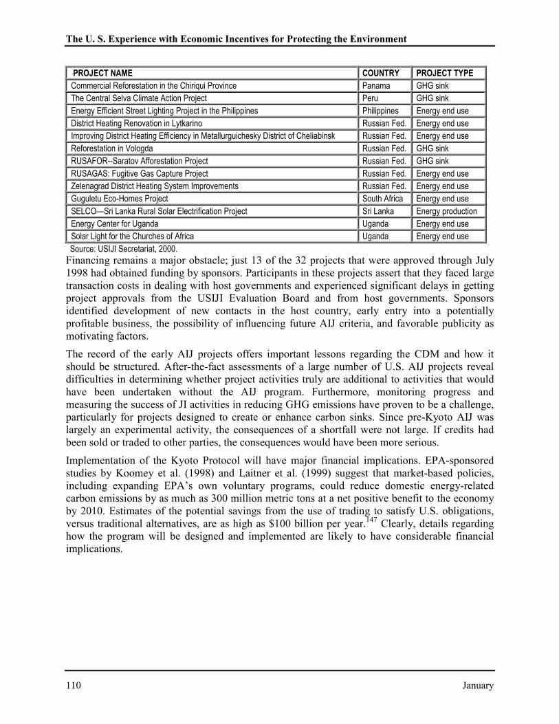
The U. S. Experience with Economic Incentives for Protecting the Environment
110 January
PROJECT NAME COUNTRY PROJECT TYPECommercial Reforestation in the Chiriqui Province Panama GHG sinkThe Central Selva Climate Action Project Peru GHG sinkEnergy Efficient Street Lighting Project in the Philippines Philippines Energy end useDistrict Heating Renovation in Lytkarino Russian Fed. Energy end useImproving District Heating Efficiency in Metallurguichesky District of Cheliabinsk Russian Fed. Energy end useReforestation in Vologda Russian Fed. GHG sinkRUSAFOR--Saratov Afforestation Project Russian Fed. GHG sinkRUSAGAS: Fugitive Gas Capture Project Russian Fed. Energy end useZelenagrad District Heating System Improvements Russian Fed. Energy end useGuguletu Eco-Homes Project South Africa Energy end useSELCO—Sri Lanka Rural Solar Electrification Project Sri Lanka Energy productionEnergy Center for Uganda Uganda Energy end useSolar Light for the Churches of Africa Uganda Energy end useSource: USIJI Secretariat, 2000.
Financing remains a major obstacle; just 13 of the 32 projects that were approved through July1998 had obtained funding by sponsors. Participants in these projects assert that they faced largetransaction costs in dealing with host governments and experienced significant delays in gettingproject approvals from the USIJI Evaluation Board and from host governments. Sponsorsidentified development of new contacts in the host country, early entry into a potentiallyprofitable business, the possibility of influencing future AIJ criteria, and favorable publicity asmotivating factors.
The record of the early AIJ projects offers important lessons regarding the CDM and how itshould be structured. After-the-fact assessments of a large number of U.S. AIJ projects revealdifficulties in determining whether project activities truly are additional to activities that wouldhave been undertaken without the AIJ program. Furthermore, monitoring progress andmeasuring the success of JI activities in reducing GHG emissions have proven to be a challenge,particularly for projects designed to create or enhance carbon sinks. Since pre-Kyoto AIJ waslargely an experimental activity, the consequences of a shortfall were not large. If credits hadbeen sold or traded to other parties, the consequences would have been more serious.
Implementation of the Kyoto Protocol will have major financial implications. EPA-sponsoredstudies by Koomey et al. (1998) and Laitner et al. (1999) suggest that market-based policies,including expanding EPA’s own voluntary programs, could reduce domestic energy-relatedcarbon emissions by as much as 300 million metric tons at a net positive benefit to the economyby 2010. Estimates of the potential savings from the use of trading to satisfy U.S. obligations,versus traditional alternatives, are as high as $100 billion per year.147 Clearly, details regardinghow the program will be designed and implemented are likely to have considerable financialimplications.