6 · web viewindifference curve, a curve that represents all different combinations of the two...

CHAPTER 6

Supply of Labor to the Economy: The Decision to Work

SUMMARY

The number of hours an individual actually works is something jointly determined by employers and employees. Chapter 5 discussed factors affecting the number of hours a firm requires its employees to work. This chapter looks at factors affecting the number of hours employees wish to work. While one may not usually think of hours of work as something individuals control, choices can be made which influence the total number of hours worked, particularly over longer time periods. The decision to participate in the labor market, the decision to seek part-time or full-time work, and the number of jobs a person works are important ways individuals affect the supply of labor. The choice of occupation will also affect an individual’s total hours, as will vacations, leaves, and absenteeism.

Two notable trends in labor force participation in the U.S. and other developed countries are the increase in the participation of women, particularly married women, and the decrease in the length of working life for men. Other trends include the decrease in the length of the workweek and changes in the flexibility of work hours. Overall, the labor force participation rate has fallen in recent years.

Given that individuals have some discretion over the supply of labor, what kinds of factors affect the choices they make? In answering this question the approach that is taken in this chapter is to view the individual’s supply of labor hours as the total time available less the individual’s demand for leisure time. Here, leisure time refers simply to any time not spent working for pay, i.e., it does not necessarily have to be time spent in a relaxing or enjoyable manner. By thinking about labor supply in this way, it is possible to analyze the demand for leisure hours—and inversely, the supply of labor—much like one would analyze the demand for food, clothing, or any other good that households regularly consume.

The standard approach to modeling consumer demand is to assume that an individual chooses between two goods so as to maximize happiness, or utility, subject to a budget constraint. Any particular level of utility can be represented graphically by an indifference curve, a curve that represents all different combinations of the two goods that yield equal satisfaction. The maximization process can be represented graphically as an individual trying to attain the highest possible indifference curve subject to a budget

1

Chapter 6: Supply of Labor

constraint. The result of this maximization process yields the demand function for each good, where this function relates the desired quantity of the good to the opportunity cost of the good, the level of household wealth, and the particular preferences of the person. In the labor supply model, the two goods are assumed to be leisure and income (which represents the consumption of all other goods at fixed prices). The demand for leisure can eventually be expressed in terms of the wage rate, the amount of nonlabor income the individual receives, and certain parameters representing the individual’s willingness to trade off leisure and income.

In constructing the individual’s labor supply curve, we ask: what happens to the number of hours the individual wishes to supply when the wage rate changes, holding all else constant? In the case of a wage increase, the opportunity cost of leisure time increases, so the number of leisure hours demanded decreases, increasing hours of labor supplied. This is called the substitution effect of a wage increase. However, as the wage rate increases, the individual is also wealthier for any given number of hours of work beyond zero. An increase in wealth allows an individual to consume more of all normal goods, including leisure, decreasing the number of hours of labor supplied. This effect of a wage increase is called the income effect.

In general, the substitution effect refers to the individual’s response to a change in the opportunity cost of the good, holding all else constant, while the income effect refers to the individual’s response to a change in wealth, holding the opportunity cost of the good constant. Since for leisure the substitution and income effects of a wage change typically oppose one another, whether the labor supply schedule is upward or downward sloping depends on the relative magnitude of the two effects. What drives the size of the income and substitution effects? Because normal preferences, with convex indifference curves, exhibit a changing marginal rate of substitution between income and leisure, the number of hours a person already works is important. Generally, the more a person is already working, the more valuable a marginal hour of leisure will be and hence the larger the income effect. The substitution effect grows larger when leisure and work hours are viewed as being highly substitutable. This could happen when the individual’s leisure time consists largely of work around the home.

Example 1

Suppose an individual ranks combinations of leisure (L) and income (Y) according to the formula

U = LY.

U denotes the utility level, or happiness ranking (higher levels of U are better), the individual places on the particular combination of leisure and income. The symbols and are constants greater than zero and represent the relative importance the individual places on leisure and income. Such a formula is called a Cobb-Douglas utility function.

2


Letting W stand for the wage rate, H the number of work hours, T the total time available, and V nonlabor income, the budget constraint an individual faces can be written as

Y = WH + V Y = W(T–L) +V.

Maximizing U subject to the budget constraint yields the following expression for the optimal value of L

L∗¿ αα+β

WT+VW

.

(For the reader with calculus training, this expression can be derived using the method of Lagrangian Multipliers; or by substituting the budget constraint into the utility function and then maximizing the resulting function.) Note that this expression applies only for the Cobb–Douglas utility function used in this example. If one changes the formula depicting preferences, the expression for the optimal value of L also changes.

Suppose the individual gives equal weight to units of leisure and income and that and are both equal to one. Assuming the analysis pertains to one month and that T = 400 hours, W = 4, and V = 400, then the optimal value for L is

L∗¿ 11+1

(4 )( 400)+4004

=250 .

This, in turn, implies that the number of hours supplied to the market (H*) is 150, and the total income of the consumer is $1,000 [(4 x 150) + 400]. This optimal combination of L and Y which yields utility level U1 is denoted by point a in Figure 6-1. The highest level of utility in this case is achieved where the indifference curve representing utility level U1

is just tangent to the budget constraint. Note that the constraint starts at $400 when H is zero, reflecting the nonlabor income of the individual. Its highest value of $2,000 (called the individual’s full income) is determined by summing the nonlabor income of the individual and his total earnings when working the maximum time of 400 hours at a wage rate of $4. The wage rate is reflected in the slope of the constraint.

What happens if the wage rate rises to $8? The slope of the budget constraint increases in magnitude showing the higher opportunity cost of leisure. The constraint also lies further to the right (except at its starting point) since the higher wage rate will imply a higher income (and wealth) at any given level of work hours. Given the preferences in this example, the individual responds by reducing leisure to 225 and increasing work hours to 175 (point b). The move from point a to b is a result of both the opportunity cost change and the income level change.

How much of the move is due to each factor? Holding the opportunity cost constant, suppose the consumer attained the higher level of utility U2 through an increase in

3


nonlabor income. In this case, the budget constraint would be the dotted line parallel to the original budget constraint (having the same wage and slope), and the optimal choice would have been point c. The movement from point a to point c is the income effect of the wage increase. Holding the level of utility constant at U2 and allowing the slope of the constraint to increase, reflecting the rise in the wage, moves the individual from point c to point b. This movement represents the substitution effect of the wage increase. Here the income and substitution effects oppose one another, but because the substitution effect is larger, the net effect of the wage increase is for leisure hours to fall and work hours to increase. The reader should note that this need not be the case, since the location of point b is determined by the preferences of the individual represented by the indifference curves. Point b must be to the left of point c, reflecting the positive substitution effect. But depending on the preferences (and the shape of the corresponding indifference curves), point b could, theoretically, end up left, right, or directly above point a.

Figure 6-1

Allowing the wage rate to vary over the entire range between $0 and $10 yields the individual labor supply schedule shown in Figure 6-2. Note that for any labor hours to be supplied the wage must be greater than one.

The lowest wage that will induce a person to participate in the labor market is called the reservation wage. When there are significant unpaid time obligations (e.g., commuting time) that accompany a job, the reservation wage will be associated with a certain minimum number of work hours.

Also note that for the preferences represented here, the substitution effect always dominates the income effect and so the curve is always upward sloping. (For differing preferences, represented by a differently shaped indifference curve mapping, the results might differ.) The wage and work hour combinations associated with the optimal points depicted in Figure 6-1 are shown again in Figure 6-2 to emphasize the close connection between the two graphs.

4


Figure 6-2

The main application of labor supply theory is to the analysis of income replacement and income maintenance programs like workers’ compensation, unemployment insurance, and welfare. By analyzing how these programs change the budget constraints, the work incentive effects of these programs can be analyzed for any given set of preferences.

For example, in some income maintenance programs, the person who does not work at all receives a subsidy S from the government, perhaps as compensation while injured or as payment of unemployment benefits. This causes a “spike” in the budget constraint, because the person receives income even when supplying zero hours of work. This program clearly has serious work disincentives; when the worker goes from zero hours to some positive number of hours, income initially drops. Second, it allows the worker to consume a bundle that contains the same amount of income but more leisure than at least one point on the original budget constraint, and that may well be preferred to other possibilities. Thus these programs stop or slow the return to work by injured or unemployed workers.

Programs such as welfare are needs-based; they pay the recipient the difference between what they earn and some standard. Thus the more income the worker earns, the lower the amount of benefits received. Benefits are scaled back by some fraction for every dollar individuals earn on their own. Letting this fraction, called the implicit tax rate, be denoted by t, where 0 t 1, then the basic budget constraint can be written as

Y = S + WH – tWH + V

Y = S + (1–t)WH + V

Y = (1–t)W(T–L) + S + V.

5


Notice that the effective wage rate (the slope of the budget constraint) becomes (1–t)W and the total level of nonlabor income (the initial height of the budget constraint) is S + V. The lower the level of t, the higher the opportunity cost of leisure, and in most instances, the stronger the incentive to work. However, the lower the level of t, the longer people remain eligible for the program, thus increasing the number of people receiving payments and thereby increasing the cost of the program. This trade-off between work incentives and program costs is a fundamental tension running through all income replacement and income maintenance programs.

The point on the budget constraint separating those who receive benefits from those who do not is called the breakeven point. Given the type of program structure mentioned above, the level of income associated with the breakeven point could be computed by finding earnings such that

S – tWH = 0 WH = .

The actual level of income at the breakeven point, of course, would be (S/t) + V.

Example 2

Consider an individual with preferences given by the formula

U=L34 Y

14 .

Assume the going wage rate is $4 per hour and that the maximum time available per month is 400 hours. Also assume initially that the person has no nonlabor income. Now suppose a welfare program provides low income individual’s with a benefit of $200 if they do not work at all. As the person earns income, however, benefits are scaled back 20 cents for every dollar earned. What would be the breakeven point of the program and what effect would such a program have on the work incentives of this individual?

The breakeven level of income would occur when the person earned enough to have the initial $200 subsidy “taken away,” that is, the total subsidy received should be zero. Algebraically, this occurs when

200 – 0.2(WH) = 0 WH = $1,000.

This would occur when the person worked 250 hours and leisure was 150 hours.

Substituting the appropriate values into the expression for the optimal level of L yields a choice of L* = 300 before the welfare program. This implies 100 work hours and a total

6


income of $400. After the adoption of the welfare program, however, the person’s nonlabor income effectively becomes S + V = $200, and the effective wage rate becomes (1–t)W = $3.20. Substituting these values into the demand function for L yields L* = 346.875 which implies work hours of 53.125. This yields total earnings of $212.50, plus a subsidy of $157.50, for a total income of $370.

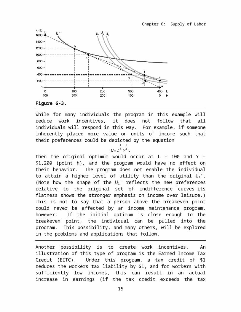
An indifference curve/budget constraint graph showing these results is plotted in Figure 6-3. The budget constraint before the welfare program is denoted by the line ab. After the welfare program is established the constraint becomes the line acdb. Note that the breakeven point of the program occurs at point d. The individual’s optimal combination of L and Y before the program was at the point e, leading to a utility level at U 1. After the program is enacted, the individual’s optimum is at point f and involves more leisure and less work (and just slightly less total income). The large gain in leisure at the cost of little income leads to the higher level of utility U2. This tendency to consume more leisure makes sense since the program creates income and substitution effects that in this case both work in the same direction to reduce work hours. Notice how the program shifts the constraint out, thus making individuals eligible for the program richer. When people are richer they typically consume more of all goods, including leisure. Notice also that the constraint is flatter, representing a lower effective wage rate, and hence a lower opportunity cost to leisure time. When the opportunity cost of a good is lower, people typically respond by substituting more of that good for the other, in this case, more leisure for less income.

While this program does reduce work incentives, it is also important to note that it does not eliminate them. This would occur, however, if the program were set up with an implicit tax rate of t = 1. The constraint then would be acgb and the person would maximize utility at point c by dropping out of the labor force entirely. As the effective wage rate goes to zero, notice the L* expression gets extremely large, but since L has a maximum of 400, that is where the optimum occurs. This is an example where the optimum does not occur at a tangency between the indifference curve and the budget constraint. Graphically, while a tangency has not been attained, the person still has reached the highest possible indifference curve consistent with the budget constraint. Notice that by dropping out of the labor force the individual would actually increase utility from U1 to U2. In general, when analyzing the work incentive effects of income maintenance programs, be sure to watch for the tendency of individuals to cluster around sharp corners on the constraint like point c. Also, note that such corner points do not necessarily occur at the end of the constraint, and sometimes the corners lack the accompanying horizontal segment between points c and g. When there is no such horizontal segment (i.e., the program pays out a subsidy only at one specific leisure value) the point is characterized in the text as a budget constraint spike.

7


Figure 6-3.

While for many individuals the program in this example will reduce work incentives, it does not follow that all individuals will respond in this way. For example, if someone inherently placed more value on units of income such that their preferences could be depicted by the equation

U=L14 Y

34 ,

then the original optimum would occur at L = 100 and Y = $1,200 (point h), and the program would have no effect on their behavior. The program does not enable the individual to attain a higher level of utility than the original U1'. (Note how the shape of the U1' reflects the new preferences relative to the original set of indifference curves—its flatness shows the stronger emphasis on income over leisure.) This is not to say that a person above the breakeven point could never be affected by an income maintenance program, however. If the initial optimum is close enough to the breakeven point, the individual can be pulled into the program. This possibility, and many others, will be explored in the problems and applications that follow.

Another possibility is to create work incentives. An illustration of this type of program is the Earned Income Tax Credit (EITC). Under this program, a tax credit of $1 reduces the workers tax liability by $1, and for workers with sufficiently low incomes, this can result in an actual increase in earnings (if the tax credit exceeds the tax liability, the government pays the worker the difference). The actual amount of the tax credit depends on both earnings and number of dependent children and is phased out as income rises. Thus there are a variety of effects, depending on the worker’s original income. For workers who work few or zero hours, the tax credit is the greatest, making the after-tax wage greater than the market wage. Thus while there are both income and substitution effects, it is likely that income effects will dominate and thus that some workers will enter the labor force or work more hours. For the middle income range, the net wage is equal to the market wage, so there is an income effect but not a substitution effect. Thus workers may actually work less. In the upper income range, the net wage is less than the market wage, as the credit is phased out. Thus the implicit reduction in the wage will create income and substitution effects, both of which will cause workers to supply less labor (because the opportunity cost of leisure has fallen while

8


income has increased), and thus it is likely that workers at that income range will choose to work less.

9


REVIEW QUESTIONS

Choose the letter that represents the BEST response.

The Labor/Leisure Choice: The Fundamentals

1. Although firms have an important say in how many hours an employee works, workers can adjust their hours through

a. choice of occupation.b. choice of full-time or part-time work.c. absenteeism.d. all of the above.

2. Indifference curves representing preferences for leisure and income should be drawn in such a way that they do not cross. If they do, it can be inferred that

a. the steeper curve represents an individual who places a low value on an extra hour of leisure.b. the individual is inconsistent in his ranking of different income and leisure combinations.c. the indifference curves that cross pertain to different individuals.d. either b or c.

In answering questions 3 and 4, please refer to Figure 6-4. The budget constraint is represented by line abc.

Figure 6-4

10


3. Which of the following is true in Figure 6-4?a. The wage rate is $4.b. Nonlabor income is $400.c. The optimal number of hours to supply is zero.d. All of the above.

4. The convex shape of the indifference curves in Figure 6-4 means thata. when leisure is low and income is high, additional units of leisure are very valuable.b. when leisure is high and income low, additional units of leisure are not very valuable.c. people generally prefer having some leisure and some income to having much income and little leisure, or much leisure and little income.d. all of the above.

5. The optimal level of leisure occurs wherea. the level of leisure is maximized subject to the budget constraint.b. the level of income is maximized subject to the budget constraint.c. the highest attainable indifference curve is tangent to the budget constraint.d. both a and b.

6. An individual with standard downward-sloping indifference curves will participate in the labor market provided

a. the indifference curves between leisure and income are steep.b. a tangency between the budget constraint and the indifference curve is reached.c. at the point where leisure is at its maximum, the indifference curve is steeper than the budget constraint.d. at the point where leisure is at its maximum, the indifference curve is flatter than the budget constraint.

In answering questions 7 and 8, please refer to Figure 6-5. The budget constraint is given by line abcd.

7. The shape of the indifference curves in Figure 6-5 means thata. after a certain number of leisure hours is reached, additional leisure hours become very valuable.b. after a certain number of leisure hours are reached, additional leisure hours have no value.c. after a certain number of leisure hours are reached, work hours are actually viewed as a good thing.d. as leisure hours increase, additional hours of leisure fall in value, but after some point, start to increase again.

11


Figure 6-5

8. Which of the following statements is consistent with Figure 6-5?a. The market wage rate is $6.b. Low income individuals receive a subsidy of $400 and face an implicit tax rate of zero.c. The optimal number of hours to supply is 50.d. The optimal number of hours to supply is zero.

Income and Substitution Effects

9. If a person has preferences that lead to a choice of zero work hours, an increase in the wage rate will result in

a. an income effect only.b. a substitution effect only.c. counteracting income and substitution effects.d. a dominant substitution effect.

10. Suppose leisure is an inferior good (a good whose consumption goes down as income goes up). As the wage rate goes up

a. hours supplied should go up.b. hours supplied should go down.c. hours supplied go up provided the substitution effect dominates the income effect.d. hours supplied go up provided the income effect dominates the substitution effect.

12


11. A backward-bending labor supply curve occurs whena. leisure is a normal good and the substitution effect dominates at low wage levels.b. leisure is a normal good and the income effect dominates at high wage levels.c. at low wages level, leisure is a normal goods, but then is an inferior good at high wage levels.d. both a and b.

12. What should be the effect on labor supply of reducing marginal income tax rates while keeping the total taxes paid by a worker constant?

a. Hours supplied should go up.b. Hours supplied will go down.c. Hours supplied stay the same.d. Hours supplied should go up if the substitution effect dominates the income effect.

Basic Income Replacement and Income Maintenance Programs

13. Suppose the government promises to pay workers who lose their sight in a workplace accident $100,000 regardless of their earnings before the accident. This payment would create

a. a pure income effect.b. a pure substitution effect.c. reinforcing income and substitution effects.d. counteracting income and substitution effects.

14. An income replacement program based on scheduled benefits generally preserves work incentives better than one that guarantees replacement of the actual income loss because the scheduled benefits approach

a. creates a pure substitution effect.b. does not alter the price of leisure.c. leads to a higher level of utility.d. overcompensates workers for their injuries.

13


In answering questions 15–18, please refer to Figure 6-6. The original constraint is line ab. The constraint associated with the income maintenance program is line acdb.

Figure 6-6

15. The implicit tax rate (t) used in this income maintenance program isa. 1.b. 0.c. 0.4.d. 0.5.

16. The actual subsidy paid to the individual will bea. $100.b. $500.c. $600.d. $1,200.

17. The substitution effect associated with this income maintenance program isa. an increase of 47 leisure hours.b. an increase of 103 leisure hours.c. a decrease of 103 leisure hours.d. an increase of 150 leisure hours.

18. The income effect associated with this income maintenance program isa. a decrease of $100.b. an increase of 47 leisure hours.c. an increase of 103 leisure hours.d. an increase of leisure hours.

14


19. In the typical income maintenance program, the higher the implicit tax ratea. the higher the breakeven point.b. the lower the work incentive.c. the higher the cost of the program.d. all of the above.

20. The problem with reducing the implicit tax rate pertaining to the welfare program is that

a. individuals well above the poverty level may receive benefits.b. the cost of the program increases.c. people will have less incentive to work.d. both a and b.

21. Under the Earned Income Tax Credit program, the theoretical effects on labor supply are ___________ for the lowest income recipients, and __________ for the highest income recipients.

a. an increase; a decreaseb. a decrease; an increasec. ambiguous; a decreased. an increase; ambiguous

22. The Earned Income Tax Credit is now viewed by many as being the most effective way of raising the incomes of the working poor because

a. it is much more closely targeted on the working poor than the minimum wage.b. the estimated impact on hours worked by the working poor is positive.c. since the subsidy comes through the tax system rather than through employers, there is no negative stigmatizing effect on recipients.d. all of the above.

PROBLEMS

The Labor/Leisure Choice: The Fundamentals

23. Suppose an individual’s preferences for leisure and income can be represented by a Cobb–Douglas utility function of the form

U = LY.

Assume the analysis pertains to one day and the maximum time available is 16 hours.

23a. Plot the U = 1,000 indifference curve assuming = 1 and = 1.

15


23b. Plot the U = 8,000 indifference curve assuming = 2 and = 1.

23c. What effect does an increased appreciation for leisure time have on the slope of a typical indifference curve?

24. Suppose the analysis pertains to one month and the maximum time available is 400 hours.

24a. Plot the budget constraint facing an individual receiving $400 in nonlabor income and a wage of $5 per hour.

24b. On the same graph, plot the budget constraint facing an individual receiving $200 in nonlabor income and a wage of $7 per hour.

Income and Substitution Effects

25. Consider Figure 6-7 which depicts a wage decrease. The original constraint is line abc. The new constraint is line abd.

Figure 6-7

25a. By how much has the wage decreased?

25b. What is the income effect of the wage decrease? What is the substitution effect of the wage decrease?

25c. Find the coordinates of two points on this individual’s labor supply curve. Is the labor supply curve upward or downward sloping over the range of the wage change?

16


Basic Income Replacement and Income Maintenance Programs

26. Consider an individual with preferences given by the formula U = LY. Suppose the total time available per day is 16 hours, the wage rate is $5, and nonlabor income is zero.

26a. Calculate the optimal level of leisure and labor hours, and the resulting earnings and utility level.

26b. Suppose the person is injured on the job in such way that he cannot work at all. Prove that a policy that compensates the worker for his lost income will increase his utility.

26c. Find the minimum percentage of income that could be replaced and just keep the worker at the same level of utility as before his injury. Do you see any problems with this analysis?

27. Consider an individual with preferences given by the formula U = LY. Assume the going wage rate is $4 per hour and that the maximum time available per month is 400 hours. Also assume initially that the person has no nonlabor income. Now suppose that a welfare program is developed that provides low income individuals with a benefit of $500 if they do not work at all. As the person earns income on his own, benefits are scaled back by the fraction t for every dollar earned.

27a. Find the change in hours supplied for each of the following implicit tax rates: t = 1, t = 0.5, t = 0.

27b. Which rate provides the least work disincentive? Explain why this happens.

28. Figure 6-8 shows two income maintenance programs that provide a maximum subsidy of $350 to anyone who does not work at all. One program is represented by the constraint acdb, while the other is represented by the constraint aceb.

17


28a. What are the implicit tax rates associated with each program?

28b. Given the preferences depicted on the graph, which program provides the strongest work incentives? Explain the intuition behind your finding.

Figure 6-8

A Variation on the Basic Income Maintenance Program

29. Consider an individual with preferences for leisure and income given by the Cobb–Douglas utility function U = LY. Suppose an income maintenance program is created where individuals who do not work receive $2,000. Those that do work also receive the full subsidy provided they earn $4,000 or less. Those earning above $4,000 have their subsidy reduced by a dollar for every additional dollar earned beyond $4,000. The maximum time available is 2,800 hours per year, and the going wage is $5. The person initially has no nonlabor income.

29a. Graph the budget constraint facing a typical individual before the program is enacted. Then draw the constraint after the program is enacted. What is the breakeven point?

29b. Find the optimal number of hours before the adoption of the program. Calculate the level of utility the individual achieves.

29c. Using the graph as a guide, find the optimal number of hours after the program is enacted. Calculate the new level of utility. Would your answer have been different if all benefits were simply cut off once a person earned $4,000?

18


APPLICATIONS

Reforming Income Maintenance and Income Replacement Programs30. A common theme in welfare reform proposals is the notion of mutual obligation. That is, society has an obligation to help the poor, but the poor also have a responsibility to strive to become self-sufficient. A concrete way in which this notion is implemented is to make the receipt of benefits conditional on the recipient first performing some task, e.g., enroll in job training or accept part-time government employment, etc.

Suppose an individual’s preferences for leisure and income can be represented by a Cobb–Douglas utility function of the form

U = LY.

Assume the going wage rate is $4 per hour and that the maximum time available per month is 400 hours. Also assume initially that the person has no nonlabor income. Concerned about the work disincentives that can accompany income maintenance programs, suppose Congress legislates that to qualify for the maximum benefit of $200 you must work 100 hours a month. Those working in excess of 100 hours will see the maximum benefit scaled back by 40 cents for each additional dollar they earn once they have qualified for the program.

30a. Draw the budget constraint facing an individual in the absence of the welfare program. Then draw the constraint with the welfare system in place. What is the breakeven point under this program?

30b. Using the graph as a guide, find the effects of the welfare program on hours worked for each of the following preference parameter combinations.1) = 0.65, = 0.35,2) = 0.75, = 0.25,3) = 0.85, = 0.15.

30c. Assess the usefulness of threshold provisions such as this in reforming welfare programs.

The Earned Income Tax Credit

31. Suppose that the Earned Income Tax Credit (EITC) program is set up so that a maximum payment of $2,700 can be earned when a qualified worker earns $9,000. This represents a payment of 30 cents for each additional dollar earned. Suppose also that workers earning between $9,000 and $12,000 are eligible for the maximum payment, but that once earnings exceed $12,000, additional earnings cause the payment to be reduced by 45 cents for each additional dollar earned.

19


Assume the maximum number of hours a person can work in a year is 3,000, and that the going wage rate is $6 per hour. Recall that individuals who do not work receive no benefits under this program.

31a. Graph the budget constraint facing a typical individual before the program is enacted. Then graph the budget constraint after the program in enacted. Be sure to find the coordinates of the point where a person is no longer eligible for the program.

31b. What is the slope of the constraint for anyone earning less than $9,000? What is the slope of the constraint for anyone earning more than $12,000?

31c. Consider a worker with preferences such that before the tax credit program she would have worked 500 hours. Is this individual likely to work more or less because of the tax credit program? How can you tell?

31d. Discuss the work incentives for someone with preferences such that before the program he worked more than 1,500 hours.

Effects of Progressive Taxes on Labor Supply

*32. Suppose an individual’s preferences for leisure and income can be represented by a Cobb–Douglas utility function of the form

U = LY.

Assume the going wage rate is $4 per hour and that the maximum time available per month is 400 hours. Also assume that the person has nonlabor income of $200. Suppose that the government raises revenue through a tax on total income. As an example, suppose that when total monthly income is $1,000 or less, income is taxed at the rate of 20 percent. Anyone with income above $1,000 must pay 20 percent on the first $1,000 they received, but also 40 percent on every dollar over $1,000. Such a system is called a progressive tax, and the two rates are called marginal tax rates. For simplicity, ignore the issue of how the tax revenues would be used.

*32a. Draw the before tax budget constraint facing an individual. Then draw the constraint with the income tax system in place.

*32b. At what point on the leisure (hours worked) axis does the 40 percent marginal tax rate begin to apply? Find the slope of the constraint to the left and to the right of this point.

*32c. Assuming a = b = 1, find the optimal hours supplied by this individual before and after the tax. What is the average tax rate the individual faces?

20


*32d. If one follows the budget line associated with the 40 percent marginal tax rate to the point where leisure is at its minimum (the full income level), it will be as if the level of nonlabor income has increased above $200. Use the value of income at this point, and the formula for full income (WT + V) to find the height of the constraint (the implicit value of V) at this point.

*32e. Assume = 1 and = 3. Using your answer to 32d, find the optimal hours supplied by this individual before and after tax. What is the average tax rate this individual faces?

*32f. Assess the consequences for labor supply of tax proposals that call for the wealthy to face significantly higher marginal tax rates.

Reducing the Costs of Working through Telecommuting

33. Consider an individual with preferences given by the formula U = LY. Assume the going wage rate is $4 per hour and that the maximum time available per month is 400 hours. Also assume initially that the person has nonlabor income of $200. Suppose the individual incurs a fixed monetary cost of $100 per month associated with working and a fixed time cost of 30 hours per month.

33a. Find the optimal amount of leisure and work that can be attained and the level of utility achieved. Verify that the level of utility is greater than that attained by not working at all.

33b. Suppose both the monetary and time costs of working are eliminated by telecommuting, that is, the person now works at home and sends her work to the office via the Internet. Find the optimal number of leisure and work hours and the level of utility achieved.

21

6 · web viewindifference curve, a curve that represents all different combinations of the two...

Documents