6.042j course notes, planar graphs
TRANSCRIPT

�� �� ......
�� �� �� ��
��� ��
��� �� ��� �
�� ��
� � ����
...........................................................................
� � �� �� �
�� �� �� � �
� � ����
� �
�
�� �
�
� �
�
�� � � �
���� � � ����
��
� � �
�. ......................................................................................................
��
Chapter 12
Planar Graphs
12.1 Drawing Graphs in the Plane
Here are three dogs and three houses.
���� ���� ����
Dog Dog Dog Can you find a path from each dog to each house such that no two paths inter
sect? A quadapus is a little-known animal similar to an octopus, but with four arms.
Here are five quadapi resting on the seafloor:
��������.............
..............................................................................
������
......................................................... ������
...............................................................................................
������
.........................................................��������
��.....................................................................................................
233
.....................................................................................................
� � � ��
� �� �
� � �� �
�� � � �
� �� �
�
�
�
�
� ���
� � � �
�
234 CHAPTER 12. PLANAR GRAPHS
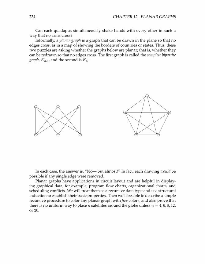
Can each quadapus simultaneously shake hands with every other in such a way that no arms cross?
Informally, a planar graph is a graph that can be drawn in the plane so that no edges cross, as in a map of showing the borders of countries or states. Thus, these two puzzles are asking whether the graphs below are planar; that is, whether they can be redrawn so that no edges cross. The first graph is called the complete bipartite graph, K3,3, and the second is K5.
�� ��� � � � ����
��� ���
����� �� ��
� � � ��
�� �������� �
�� �� �
�� �
�� ��� � � ����� �
���� ��
���� ������� � �
�� ���
In each case, the answer is, “No— but almost!” In fact, each drawing would be possible if any single edge were removed.
Planar graphs have applications in circuit layout and are helpful in displaying graphical data, for example, program flow charts, organizational charts, and scheduling conflicts. We will treat them as a recursive data type and use structural induction to establish their basic properties. Then we’ll be able to describe a simple recursive procedure to color any planar graph with five colors, and also prove that there is no uniform way to place n satellites around the globe unless n = 4, 6, 8, 12, or 20.
235 12.2. CONTINUOUS & DISCRETE FACES
When wires are arranged on a surface, like a circuit board or microchip, crossings require troublesome three-dimensional structures. When Steve Wozniak designed the disk drive for the early Apple II computer, he struggled mightly to achieve a nearly planar design:
For two weeks, he worked late each night to make a satisfactory design. When he was finished, he found that if he moved a connector he could cut down on feedthroughs, making the board more reliable. To make that move, however, he had to start over in his design. This time it only took twenty hours. He then saw another feedthrough that could be eliminated, and again started over on his design. ”The final design was generally recognized by computer engineers as brilliant and was by engineering aesthetics beautiful. Woz later said, ’It’s something you can only do if you’re the engineer and the PC board layout person yourself. That was an artistic layout. The board has virtually no feedthroughs.’”a
aFrom apple2history.org which in turn quotes Fire in the Valley by Freiberger and Swaine.
12.2 Continuous & Discrete Faces
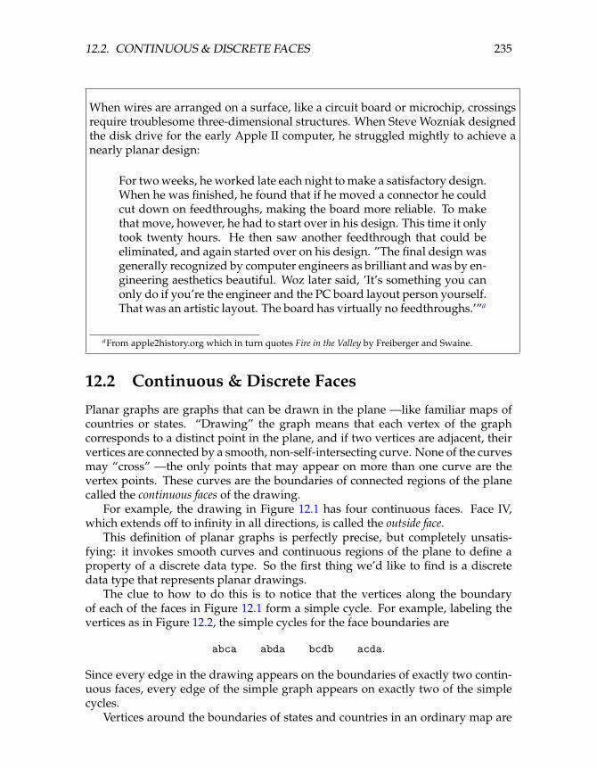
Planar graphs are graphs that can be drawn in the plane —like familiar maps of countries or states. “Drawing” the graph means that each vertex of the graph corresponds to a distinct point in the plane, and if two vertices are adjacent, their vertices are connected by a smooth, non-self-intersecting curve. None of the curves may “cross” —the only points that may appear on more than one curve are the vertex points. These curves are the boundaries of connected regions of the plane called the continuous faces of the drawing.
For example, the drawing in Figure 12.1 has four continuous faces. Face IV, which extends off to infinity in all directions, is called the outside face.
This definition of planar graphs is perfectly precise, but completely unsatisfying: it invokes smooth curves and continuous regions of the plane to define a property of a discrete data type. So the first thing we’d like to find is a discrete data type that represents planar drawings.
The clue to how to do this is to notice that the vertices along the boundary of each of the faces in Figure 12.1 form a simple cycle. For example, labeling the vertices as in Figure 12.2, the simple cycles for the face boundaries are
abca abda bcdb acda.
Since every edge in the drawing appears on the boundaries of exactly two continuous faces, every edge of the simple graph appears on exactly two of the simple cycles.
Vertices around the boundaries of states and countries in an ordinary map are
236 CHAPTER 12. PLANAR GRAPHS
Figure 12.1: A Planar Drawing with Four Faces.
IV IIIII
a
b
cd
Figure 12.2: The Drawing with Labelled Vertices.
always simple cycles, but oceans are slightly messier. The ocean boundary is the set of all boundaries of islands and continents in the ocean; it is a set of simple cycles (this can happen for countries too —like Bangladesh). But this happens because islands (and the two parts of Bangladesh) are not connected to each other. So we can dispose of this complication by treating each connected component separately.
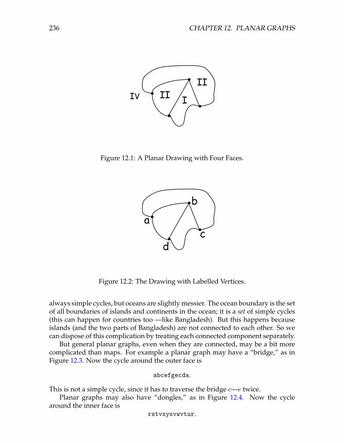
But general planar graphs, even when they are connected, may be a bit more complicated than maps. For example a planar graph may have a “bridge,” as in Figure 12.3. Now the cycle around the outer face is
abcefgecda.
This is not a simple cycle, since it has to traverse the bridge c—e twice. Planar graphs may also have “dongles,” as in Figure 12.4. Now the cycle
around the inner face is rstvxyxvwvtur,
237
Figure 12.3: A Planar Drawing with a Bridge.
12.3. PLANAR EMBEDDINGS
a
d
bc
g
f
e
rt
s
u
y x
wv
Figure 12.4: A Planar Drawing with a Dongle.
because it has to traverse every edge of the dongle twice —once “coming” and once “going.”
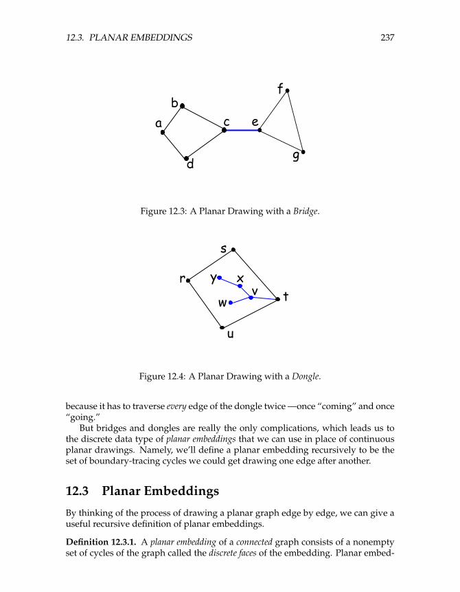
But bridges and dongles are really the only complications, which leads us to the discrete data type of planar embeddings that we can use in place of continuous planar drawings. Namely, we’ll define a planar embedding recursively to be the set of boundary-tracing cycles we could get drawing one edge after another.
12.3 Planar Embeddings
By thinking of the process of drawing a planar graph edge by edge, we can give a useful recursive definition of planar embeddings.
Definition 12.3.1. A planar embedding of a connected graph consists of a nonempty set of cycles of the graph called the discrete faces of the embedding. Planar embed
238 CHAPTER 12. PLANAR GRAPHS
dings are defined recursively as follows:
• Base case: If G is a graph consisting of a single vertex, v, then a planar embedding of G has one discrete face, namely the length zero cycle, v.
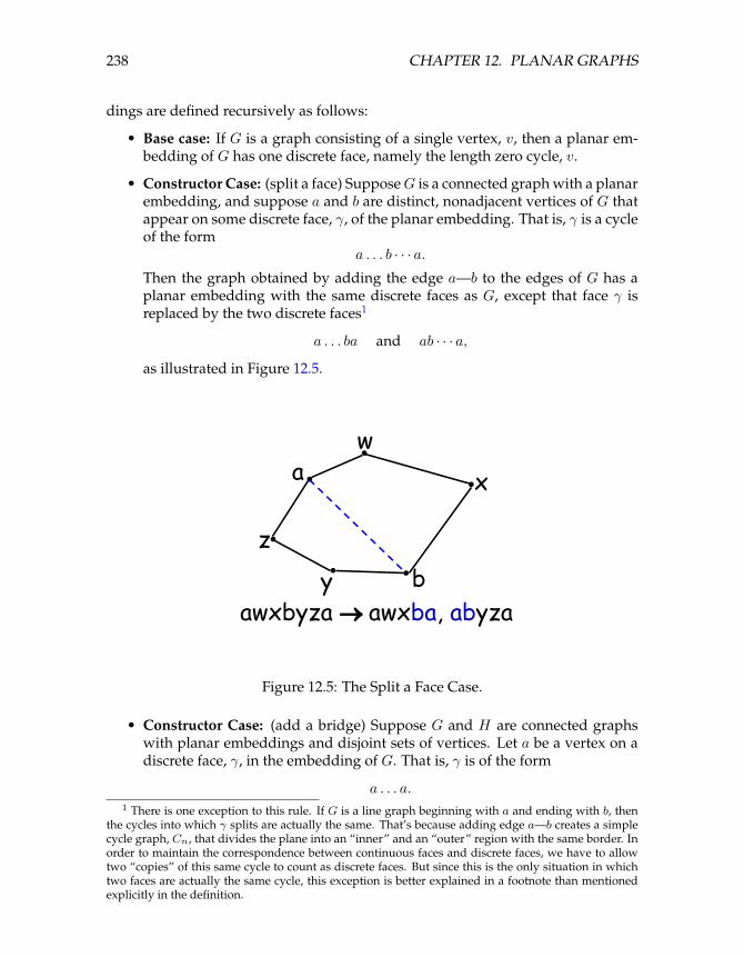
• Constructor Case: (split a face) Suppose G is a connected graph with a planar embedding, and suppose a and b are distinct, nonadjacent vertices of G that appear on some discrete face, γ, of the planar embedding. That is, γ is a cycle of the form
a . . . b a.· · · Then the graph obtained by adding the edge a—b to the edges of G has a planar embedding with the same discrete faces as G, except that face γ is replaced by the two discrete faces1
a . . . ba and ab · · · a,
as illustrated in Figure 12.5.
a
z
y b
x
w
awxbyza → awxba, abyza
Figure 12.5: The Split a Face Case.
• Constructor Case: (add a bridge) Suppose G and H are connected graphs with planar embeddings and disjoint sets of vertices. Let a be a vertex on a discrete face, γ, in the embedding of G. That is, γ is of the form
a . . . a. 1 There is one exception to this rule. If G is a line graph beginning with a and ending with b, then
the cycles into which γ splits are actually the same. That’s because adding edge a—b creates a simple cycle graph, Cn, that divides the plane into an “inner” and an “outer” region with the same border. In order to maintain the correspondence between continuous faces and discrete faces, we have to allow two “copies” of this same cycle to count as discrete faces. But since this is the only situation in which two faces are actually the same cycle, this exception is better explained in a footnote than mentioned explicitly in the definition.

axyza, btuvwb → axyzabtuvwba
y
x
za
ut
b
vw
239 12.3. PLANAR EMBEDDINGS
Similarly, let b be a vertex on a discrete face, δ, in the embedding of H , so δ is of the form
b b.· · ·
Then the graph obtained by connecting G and H with a new edge, a—b, has a planar embedding whose discrete faces are the union of the discrete faces of G and H , except that faces γ and δ are replaced by one new face
a . . . ab ba.· · ·
This is illustrated in Figure 12.6, where the faces of G and H are:
G : {axyza, axya, ayza} H : {btuvwb, btvwb, tuvt} ,
and after adding the bridge a—b, there is a single connected graph with faces
{axyzabtuvwba, axya, ayza, btvwb, tuvt} .
Figure 12.6: The Add Bridge Case.
An arbitrary graph is planar iff each of its connected components has a planar embedding.
240 CHAPTER 12. PLANAR GRAPHS
12.4 What outer face?
Notice that the definition of planar embedding does not distinguish an “outer” face. There really isn’t any need to distinguish one.
In fact, a planar embedding could be drawn with any given face on the outside. An intuitive explanation of this is to think of drawing the embedding on a sphere instead of the plane. Then any face can be made the outside face by “puncturing” that face of the sphere, stretching the puncture hole to a circle around the rest of the faces, and flattening the circular drawing onto the plane.
So pictures that show different “outside” boundaries may actually be illustrations of the same planar embedding.
This is what justifies the “add bridge” case in a planar embedding: whatever face is chosen in the embeddings of each of the disjoint planar graphs, we can draw a bridge between them without needing to cross any other edges in the drawing, because we can assume the bridge connects two “outer” faces.
12.5 Euler’s Formula
The value of the recursive definition is that it provides a powerful technique for proving properties of planar graphs, namely, structural induction.
One of the most basic properties of a connected planar graph is that its number of vertices and edges determines the number of faces in every possible planar embedding:
Theorem 12.5.1 (Euler’s Formula). If a connected graph has a planar embedding, then
v − e + f = 2
where v is the number of vertices, e is the number of edges, and f is the number of faces.
For example, in Figure 12.1, |V | = 4, |E| = 6, and f = 4. Sure enough, 4−6+4 = 2, as Euler’s Formula claims.
Proof. The proof is by structural induction on the definition of planar embeddings. Let P (E) be the proposition that v − e + f = 2 for an embedding, E .
Base case: (E is the one vertex planar embedding). By definition, v = 1, e = 0, and f = 1, so P (E) indeed holds.
Constructor case: (split a face) Suppose G is a connected graph with a planar embedding, and suppose a and b are distinct, nonadjacent vertices of G that appear on some discrete face, γ = a . . . b a, of the planar embedding. · · ·
Then the graph obtained by adding the edge a—b to the edges of G has a planar embedding with one more face and one more edge than G. So the quantity v − e + f will remain the same for both graphs, and since by structural induction this quantity is 2 for G’s embedding, it’s also 2 for the embedding of G with the added edge. So P holds for the constructed embedding.
�
241 12.6. NUMBER OF EDGES VERSUS VERTICES
Constructor case: (add bridge) Suppose G and H are connected graphs with planar embeddings and disjoint sets of vertices. Then connecting these two graphs with a bridge merges the two bridged faces into a single face, and leaves all other faces unchanged. So the bridge operation yields a planar embedding of a connected graph with vG + vH vertices, eG + eH + 1 edges, and fG + fH − 1 faces. But
(vG + vH ) − (eG + eH + 1) + (fG + fH − 1) = (vG − eG + fG) + (vH − eH + fH ) − 2
= (2) + (2) − 2 (by structural induction hypothesis) = 2.
So v −e+f remains equal to 2 for the constructed embedding. That is, P also holds in this case.
This completes the proof of the constructor cases, and the theorem follows by structural induction. �
12.6 Number of Edges versus Vertices
Like Euler’s formula, the following lemmas follow by structural induction directly from the definition of planar embedding.
Lemma 12.6.1. In a planar embedding of a connected graph, each edge is traversed once by each of two different faces, or is traversed exactly twice by one face.
Lemma 12.6.2. In a planar embedding of a connected graph with at least three vertices, each face is of length at least three.
Corollary 12.6.3. Suppose a connected planar graph has v ≥ 3 vertices and e edges. Then
e ≤ 3v − 6.
Proof. By definition, a connected graph is planar iff it has a planar embedding. So suppose a connected graph with v vertices and e edges has a planar embedding with f faces. By Lemma 12.6.1, every edge is traversed exactly twice by the face boundaries. So the sum of the lengths of the face boundaries is exactly 2e. Also by Lemma 12.6.2, when v ≥ 3, each face boundary is of length at least three, so this sum is at least 3f . This implies that
3f ≤ 2e. (12.1)
But f = e − v + 2 by Euler’s formula, and substituting into (12.1) gives
3(e − v + 2) ≤ 2e
e − 3v + 6 ≤ 0
e ≤ 3v − 6
242 CHAPTER 12. PLANAR GRAPHS
Corollary 12.6.3 lets us prove that the quadapi can’t all shake hands without crossing. Representing quadapi by vertices and the necessary handshakes by edges, we get the complete graph, K5. Shaking hands without crossing amounts to showing that K5 is planar. But K5 is connected, has 5 vertices and 10 edges, and 10 > 3 5 − 6. This violates the condition of Corollary 12.6.3 required for K5 to be · planar, which proves
Lemma 12.6.4. K5 is not planar.
Another consequence is
Lemma 12.6.5. Every planar graph has a vertex of degree at most five.
Proof. If every vertex had degree at least 6, then the sum of the vertex degrees is at least 6v, but since the sum equals 2e, we have e ≥ 3v contradicting the fact that e ≤ 3v − 6 < 3v by Corollary 12.6.3. �
12.7 Planar Subgraphs
If you draw a graph in the plane by repeatedly adding edges that don’t cross, you clearly could add the edges in any other order and still wind up with the same drawing. This is so basic that we might presume that our recursively defined planar embeddings have this property. But that wouldn’t be fair: we really need to prove it. After all, the recursive definition of planar embedding was pretty technical —maybe we got it a little bit wrong, with the result that our embeddings don’t have this basic draw-in-any-order property.
Now any ordering of edges can be obtained just by repeatedly switching the order of successive edges, and if you think about the recursive definition of embedding for a minute, you should realize that you can switch any pair of successive edges if you can just switch the last two. So it all comes down to the following lemma.
Lemma 12.7.1. Suppose that, starting from some embeddings of planar graphs with disjoint sets of vertices, it is possible by two successive applications of constructor operations to add edges e and then f to obtain a planar embedding, F . Then starting from the same embeddings, it is also possible to obtain F by adding f and then e with two successive applications of constructor operations.
We’ll leave the proof of Lemma 12.7.1 to Problem 12.6.
Corollary 12.7.2. Suppose that, starting from some embeddings of planar graphs with disjoint sets of vertices, it is possible to add a sequence of edges e0, e1, . . . , en by successive applications of constructor operations to obtain a planar embedding, F . Then starting from the same embeddings, it is also possible to obtain F by applications of constructor operations that successively add any permutation2 of the edges e0, e1, . . . , en.
2If π : {0, 1, . . . , n} → {0, 1, . . . , n} is a bijection, then the sequence eπ(0), eπ(1), . . . , eπ(n) is called a permutation of the sequence e0, e1, . . . , en.
243 12.8. PLANAR 5-COLORABILITY
Corollary 12.7.3. Deleting an edge from a planar graph leaves a planar graph.
Proof. By Corollary 12.7.2, we may assume the deleted edge was the last one added in constructing an embedding of the graph. So the embedding to which this last edge was added must be an embedding of the graph without that edge. �
Since we can delete a vertex by deleting all its incident edges, Corollary 12.7.3 immediately implies
Corollary 12.7.4. Deleting a vertex from a planar graph, along with all its incident edges of course, leaves another planar graph.
A subgraph of a graph, G, is any graph whose set of vertices is a subset of the vertices of G and whose set of edges is a subset of the set of edges of G. So we can summarize Corollaries 12.7.3 and 12.7.4 and their consequences in a Theorem.
Theorem 12.7.5. Any subgraph of a planar graph is planar.
12.8 Planar 5-Colorability
We need to know one more property of planar graphs in order to prove that planar graphs are 5-colorable.
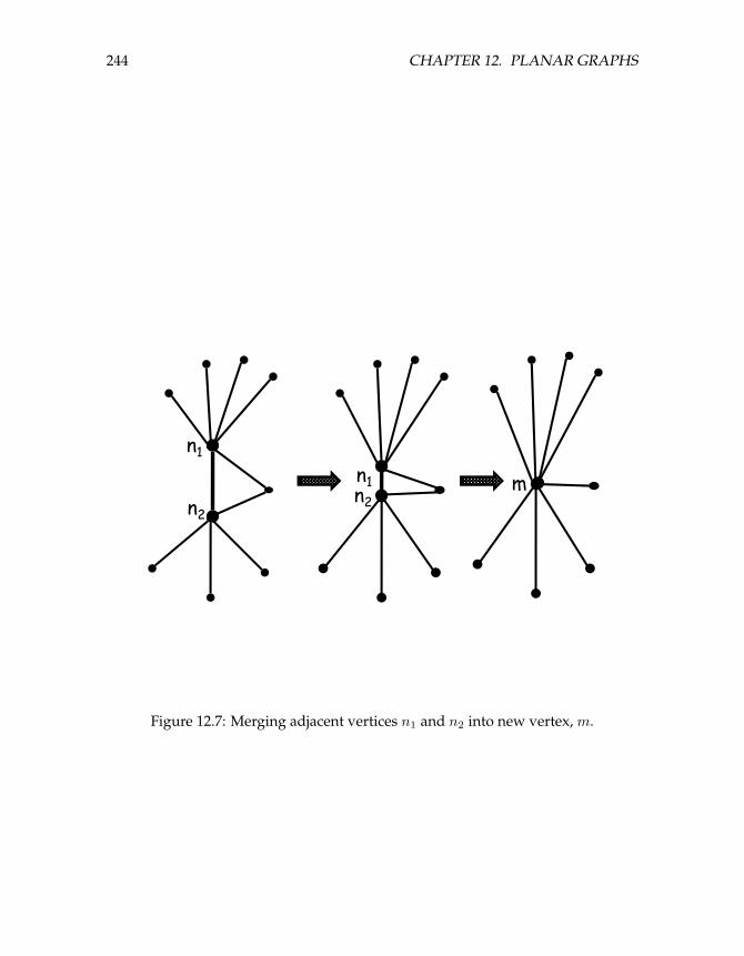
Lemma 12.8.1. Merging two adjacent vertices of a planar graph leaves another planar graph.
Here merging two adjacent vertices, n1 and n2 of a graph means deleting the two vertices and then replacing them by a new “merged” vertex, m, adjacent to all the vertices that were adjacent to either of n1 or n2, as illustrated in Figure 12.7.
Lemma 12.8.1 can be proved by structural induction, but the proof is kind of boring, and we hope you’ll be relieved that we’re going to omit it. (If you insist, we can add it to the next problem set.)
Now we’ve got all the simple facts we need to prove 5-colorability.
Theorem 12.8.2. Every planar graph is five-colorable.
Proof. The proof will be by strong induction on the number, v, of vertices, with induction hypothesis:
Every planar graph with v vertices is five-colorable.
Base cases (v ≤ 5): immediate. Inductive case: Suppose G is a planar graph with v + 1 vertices. We will de
scribe a five-coloring of G. First, choose a vertex, g, of G with degree at most 5; Lemma 12.6.5 guarantees
there will be such a vertex. Case 1 (deg (g) < 5): Deleting g from G leaves a graph, H , that is planar by
Lemma 12.7.4, and, since H has v vertices, it is five-colorable by induction hypothesis. Now define a five coloring of G as follows: use the five-coloring of H for all
244 CHAPTER 12. PLANAR GRAPHS
n11
n n2n1 m
n2
Figure 12.7: Merging adjacent vertices n1 and n2 into new vertex, m.
�
245 12.9. CLASSIFYING POLYHEDRA
the vertices besides g, and assign one of the five colors to g that is not the same as the color assigned to any of its neighbors. Since there are fewer than 5 neighbors, there will always be such a color available for g.
Case 2 (deg (g) = 5): If the five neighbors of g in G were all adjacent to each other, then these five vertices would form a nonplanar subgraph isomorphic to K5, contradicting Theorem 12.7.5. So there must be two neighbors, n1 and n2, of g that are not adjacent. Now merge n1 and g into a new vertex, m, as in Figure 12.7. In this new graph, n2 is adjacent to m, and the graph is planar by Lemma 12.8.1. So we can then merge m and n2 into a another new vertex, m�, resulting in a new graph, G�, which by Lemma 12.8.1 is also planar. Now G� has v − 1 vertices and so is five-colorable by the induction hypothesis.
Now define a five coloring of G as follows: use the five-coloring of G� for all the vertices besides g, n1 and n2. Next assign the color of m� in G� to be the color of the neighbors n1 and n2. Since n1 and n2 are not adjacent in G, this defines a proper five-coloring of G except for vertex g. But since these two neighbors of g have the same color, the neighbors of g have been colored using fewer than five colors altogether. So complete the five-coloring of G by assigning one of the five colors to g that is not the same as any of the colors assigned to its neighbors.
A graph obtained from a graph, G, be repeatedly deleting vertices, deleting edges, and merging adjacent vertices is called a minor of G. Since K5 and K3,3 are not planar, Lemmas 12.7.3, 12.7.4, and 12.8.1 immediately imply:
Corollary 12.8.3. A graph which has K5 or K3,3 as a minor is not planar.
We don’t have time to prove it, but the converse of Corollary 12.8.3 is also true. This gives the following famous, very elegant, and purely discrete characterization of planar graphs:
Theorem 12.8.4 (Kuratowksi). A graph is not planar iff it has K5 or K3,3 as a minor.
12.9 Classifying Polyhedra
The Pythagoreans had two great mathematical secrets, the irrationality of √
2 and a geometric construct that we’re about to rediscover!
A polyhedron is a convex, three-dimensional region bounded by a finite number of polygonal faces. If the faces are identical regular polygons and an equal number of polygons meet at each corner, then the polyhedron is regular. Three examples of regular polyhedra are shown below: the tetrahedron, the cube, and the octahedron.

� � � � � � � � � �� �� � �� �
� � �� � �
�
� �
� �
246 CHAPTER 12. PLANAR GRAPHS
We can determine how many more regular polyhedra there are by thinking about planarity. Suppose we took any polyhedron and placed a sphere inside it. Then we could project the polyhedron face boundaries onto the sphere, which would give an image that was a planar graph embedded on the sphere, with the images of the corners of the polyhedron corresponding to vertices of the graph. But we’ve already observed that embeddings on a sphere are the same as embed-dings on the plane, so Euler’s formula for planar graphs can help guide our search for regular polyhedra.
For example, planar embeddings of the three polyhedra above look like this:
����� ���
�� ��� ��
����
���
�������� � � ����������� �����
Let m be the number of faces that meet at each corner of a polyhedron, and let n be the number of sides on each face. In the corresponding planar graph, there are m edges incident to each of the v vertices. Since each edge is incident to two vertices, we know:
mv = 2e
Also, each face is bounded by n edges. Since each edge is on the boundary of two faces, we have:
nf = 2e
Solving for v and f in these equations and then substituting into Euler’s formula gives:
2e 2e m − e + = 2
n
which simplifies to 1 1 1 1
+ = + (12.2) m n e 2
This last equation (12.2) places strong restrictions on the structure of a polyhedron. Every nondegenerate polygon has at least 3 sides, so n ≥ 3. And at least 3 polygons must meet to form a corner, so m ≥ 3. On the other hand, if either n or m were 6 or more, then the left side of the equation could be at most 1/3 + 1/6 = 1/2, which
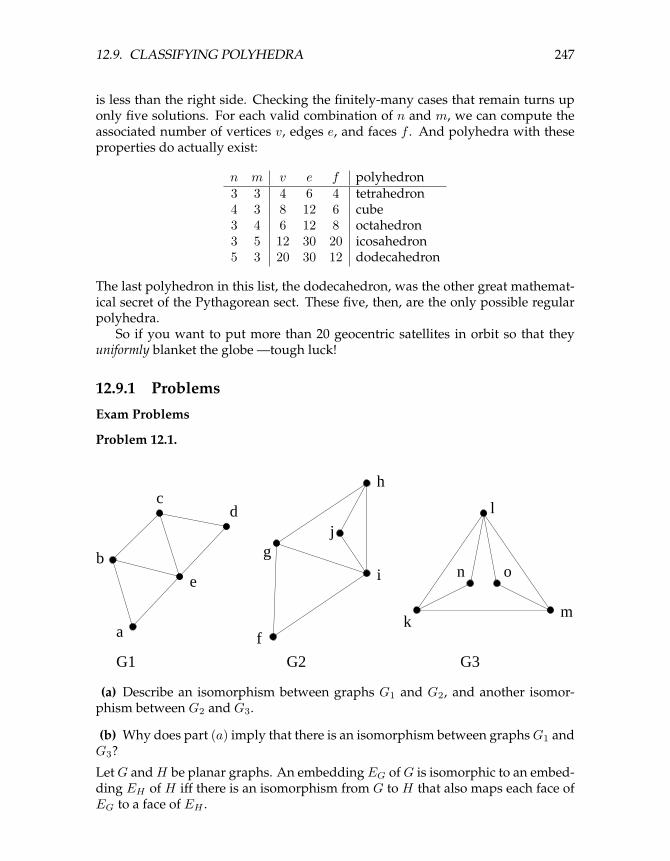
247 12.9. CLASSIFYING POLYHEDRA
is less than the right side. Checking the finitely-many cases that remain turns up only five solutions. For each valid combination of n and m, we can compute the associated number of vertices v, edges e, and faces f . And polyhedra with these properties do actually exist:
n m 3 3 4 6 4 tetrahedron 4 3 8 12 6 cube 3 4 6 12 8 octahedron 3 5 12 30 20 icosahedron 5 3 20 30 12 dodecahedron
v e f polyhedron
The last polyhedron in this list, the dodecahedron, was the other great mathematical secret of the Pythagorean sect. These five, then, are the only possible regular polyhedra.
So if you want to put more than 20 geocentric satellites in orbit so that they uniformly blanket the globe —tough luck!
12.9.1 Problems
Exam Problems
Problem 12.1.
k
n
l
o
m
gj
h
i
f
c
b
a
e
d
G1 G2 G3
(a) Describe an isomorphism between graphs G1 and G2, and another isomorphism between G2 and G3.
(b) Why does part (a) imply that there is an isomorphism between graphs G1 and G3?
Let G and H be planar graphs. An embedding EG of G is isomorphic to an embedding EH of H iff there is an isomorphism from G to H that also maps each face ofEG to a face of EH .
248 CHAPTER 12. PLANAR GRAPHS
(c) One of the embeddings pictured above is not isomorphic to either of the others. Which one? Briefly explain why.
(d) Explain why all embeddings of two isomorphic planar graphs must have the same number of faces.
Class Problems
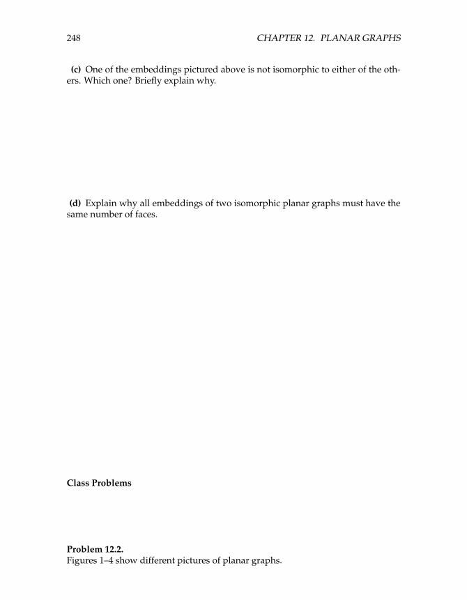
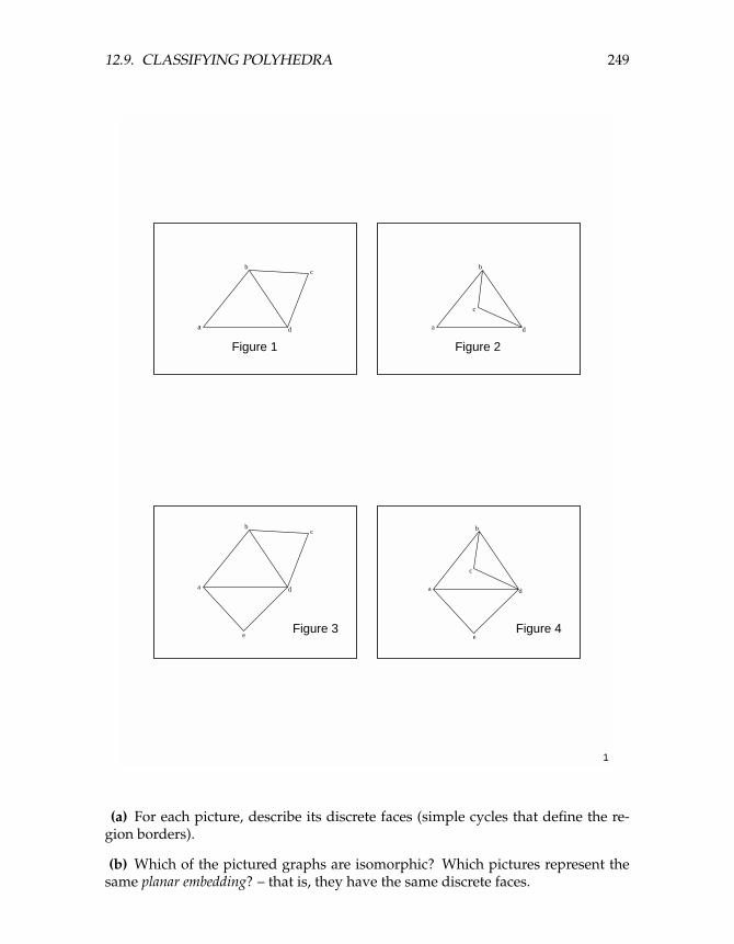
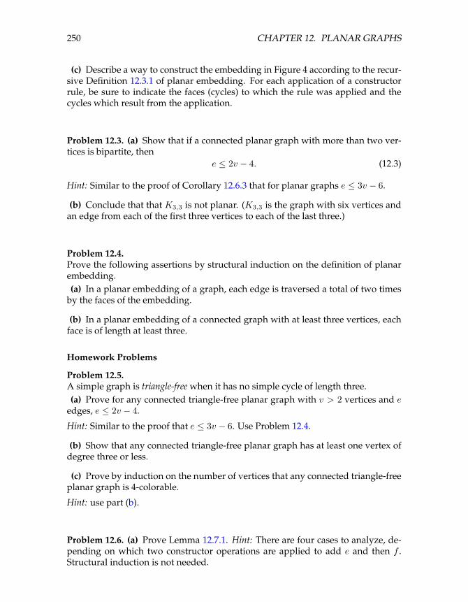
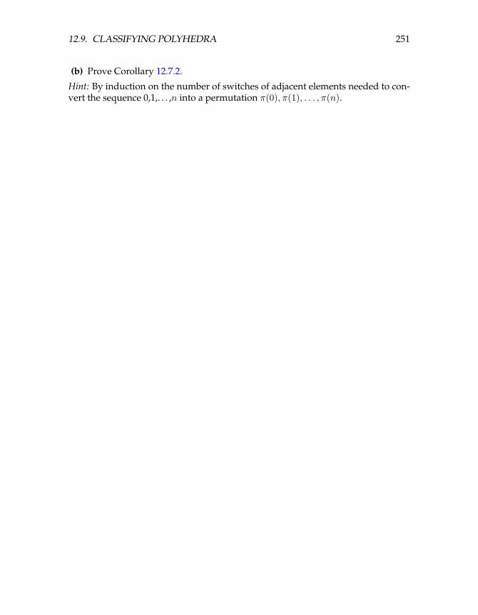
Problem 12.2. Figures 1–4 show different pictures of planar graphs.
249 12.9. CLASSIFYING POLYHEDRA
1
a
bc
d
Figure 1
a
b
c
d
Figure 2
a
bc
d
eFigure 3
a
b
c
d
eFigure 4
(a) For each picture, describe its discrete faces (simple cycles that define the region borders).
(b) Which of the pictured graphs are isomorphic? Which pictures represent the same planar embedding? – that is, they have the same discrete faces.
250 CHAPTER 12. PLANAR GRAPHS
(c) Describe a way to construct the embedding in Figure 4 according to the recursive Definition 12.3.1 of planar embedding. For each application of a constructor rule, be sure to indicate the faces (cycles) to which the rule was applied and the cycles which result from the application.
Problem 12.3. (a) Show that if a connected planar graph with more than two vertices is bipartite, then
e ≤ 2v − 4. (12.3)
Hint: Similar to the proof of Corollary 12.6.3 that for planar graphs e ≤ 3v − 6.
(b) Conclude that that K3,3 is not planar. (K3,3 is the graph with six vertices and an edge from each of the first three vertices to each of the last three.)
Problem 12.4. Prove the following assertions by structural induction on the definition of planar embedding. (a) In a planar embedding of a graph, each edge is traversed a total of two times
by the faces of the embedding.
(b) In a planar embedding of a connected graph with at least three vertices, each face is of length at least three.
Homework Problems
Problem 12.5. A simple graph is triangle-free when it has no simple cycle of length three. (a) Prove for any connected triangle-free planar graph with v > 2 vertices and e
edges, e ≤ 2v − 4.
Hint: Similar to the proof that e ≤ 3v − 6. Use Problem 12.4.
(b) Show that any connected triangle-free planar graph has at least one vertex of degree three or less.
(c) Prove by induction on the number of vertices that any connected triangle-free planar graph is 4-colorable.
Hint: use part (b).
Problem 12.6. (a) Prove Lemma 12.7.1. Hint: There are four cases to analyze, depending on which two constructor operations are applied to add e and then f . Structural induction is not needed.
251 12.9. CLASSIFYING POLYHEDRA
(b) Prove Corollary 12.7.2.
Hint: By induction on the number of switches of adjacent elements needed to convert the sequence 0,1,. . . ,n into a permutation π(0), π(1), . . . , π(n).
252 CHAPTER 12. PLANAR GRAPHS

MIT OpenCourseWarehttp://ocw.mit.edu
6.042J / 18.062J Mathematics for Computer Science Spring 2010
For information about citing these materials or our Terms of Use, visit: http://ocw.mit.edu/terms.