6.1. introduction - lneg - laboratório nacional de ... · relation is proposed between these...
TRANSCRIPT

Chapter 6. Shelf sedimentary dynamics
6.1. Introduction
The superficial sedimentary cover of the Faial shelf is described in this
chapter and the reasons for its peculiar sedimentary pattern are discussed. The
seaward limits of the cross-shore transport of sediments are estimated and a
relation is proposed between these limits and the cross-shore sedimentary
variation. The longshore transport of sediments is calculated for the sectors with
nearshore sediments and simple bathymetry. All these characterizations aim to
understand the present-day shelf dynamics and to help in the evaluation of these
sediments as aggregates and limit their potential dredging areas in Chapter 7.
6.2. Characterization of the shelf sedimentary
environments
One of the main purposes of this investigation was to study the part of the
insular shelf of Faial that is composed of sand and gravel. For that purpose Box-
Core samples were collected between 20 and 80 meters water depth (see Figure
14 in Chapter 1) in order to study the distribution patterns of sediment texture and
composition. The samples were taken along cross-shore transects spaced
between 300 and 1000 m, up to 80 m offshore and along-shore transects spaced
between 1000 and 4000m. The grid sampling was chosen to be irregular because
it was adjusted according to the specific characteristics of each shelf sector, based
on the interpretation of the seismic and bathymetric data. For each of the samples
several statistical parameters were calculated. The mean, sorting, skewness and
kurtosis were calculated using the moment measures on the whole sediment
distribution using the Folk and Ward method (1957). For that purpose the Visual
Basic program GSSTAT (Poppe et al., 2004), available from the International
Association for Mathematical Geology web-site was used to calculate these
225
The insular shelf of Faial: Morphological and sedimentary evolution
moment statistics. The Visual Basic program SEDCLASS (Poppe et al., 2003),
also available from the International Association for Mathematical Geology web-
site was used to generate automatically the Folk’s classification system of
sediments (1954) based on gravel-sand-silt-clay ratios.
6.2.1. The shelf grain-size distribution
Table 13 presents the percentages of each size fraction in the samples
using the phi scale defined by Krumbein (1938) and the Folk’s classification
system (1954) based on gravel-sand-silt-clay ratios, while Table 14 presents the
corresponding moment statistics (mean, sorting, skewness and kurtosis,
respectively M1, M2, M3 and M4), the description of the samples based on the
moment statistics classification of Folk (1974) and the carbonate calcium
percentage of each sample.
A brief analysis of the results shows that there are no samples finer than
medium sands (Table 14 and Figure 169). In fact, 54% of the samples collected
revealed sediments that are medium sands, 17% that are coarse sands, 26% that
are very coarse sands and 3% that are granules according to the Udden-
Wentworth scale (1922). Moreover, when using the Folk’s classification ternary
diagram (1954), 54% of the samples fall into the category of slightly gravely sand,
34% fall into gravely sand and 12% into sandy gravel (Table 13 and Figure 170).
Apparently, the presence of coarse sediments in the Faial shelf points out to a
rather energetic depositional environment as already discussed in section 2.4.4 of
Chapter 2 and section 4.3.7 of Chapter 4.
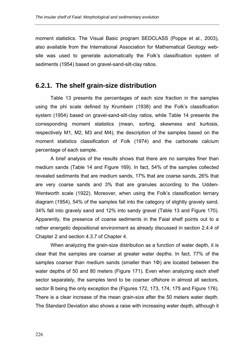
When analyzing the grain-size distribution as a function of water depth, it is
clear that the samples are coarser at greater water depths. In fact, 77% of the
samples coarser than medium sands (smaller than 1Φ) are located between the
water depths of 50 and 80 meters (Figure 171). Even when analyzing each shelf
sector separately, the samples tend to be coarser offshore in almost all sectors,
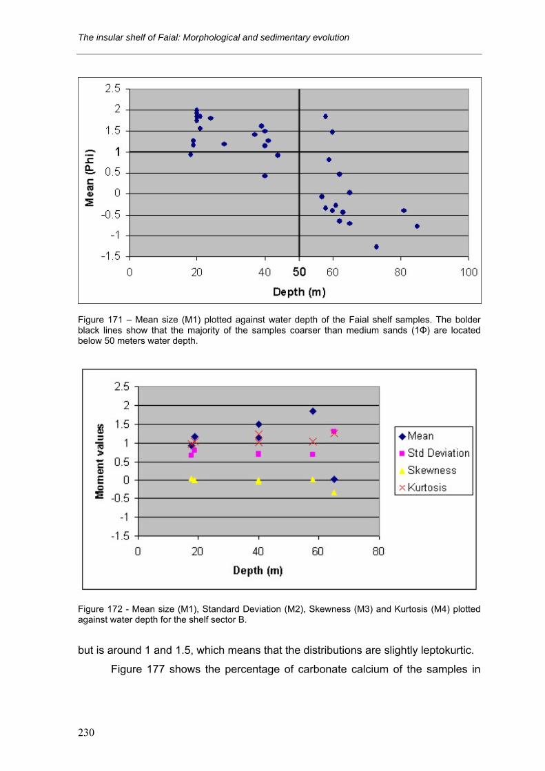
sector B being the only exception the (Figures 172, 173, 174, 175 and Figure 176).
There is a clear increase of the mean grain-size after the 50 meters water depth.
The Standard Deviation also shows a raise with increasing water depth, although it
226

Chapter 6. Shelf sedimentary dynamics
is not so clear in some shelf sectors. The Skewness is fairly constant around the 0
value, which means that the sediment distribution is nearly symmetrical in all the
cases, resembling a normal Gaussian curve. The Kurtosis value is less constant
Figure 169 – Mean grain size (M1) distribution of the samples in the shelf. The rocky outcrops correspond to the lava flows and coarse clastic deposits interpreted in Chapter 3.
A B Figure 170 – A: Folk’s (1954) classification ternary diagram. B: Folk’s (1954) classification of the Faial shelf samples showing that these have a significant percentage of gravels.
227

The insular shelf of Faial: Morphological and sedimentary evolution
228

Chapter 6. Shelf sedimentary dynamics
229
The insular shelf of Faial: Morphological and sedimentary evolution
Figure 171 – Mean size (M1) plotted against water depth of the Faial shelf samples. The bolder black lines show that the majority of the samples coarser than medium sands (1Φ) are located below 50 meters water depth.
Figure 172 - Mean size (M1), Standard Deviation (M2), Skewness (M3) and Kurtosis (M4) plotted against water depth for the shelf sector B.
but is around 1 and 1.5, which means that the distributions are slightly leptokurtic.
Figure 177 shows the percentage of carbonate calcium of the samples in
230

Chapter 6. Shelf sedimentary dynamics
the shelf, which is due to the presence of carbonate skeletal particles. It is
however difficult to explain why there is such variability along the shelf due to the
absence of habitat mapping in the Faial shelf.
Figure 173 - Mean size (M1), Standard Deviation (M2), Skewness (M3) and Kurtosis (M4) plotted against water depth for the shelf sectors C and D.
Figure 174 - Mean size (M1), Standard Deviation (M2), Skewness (M3) and Kurtosis (M4) plotted against water depth for the shelf sector E.
231
The insular shelf of Faial: Morphological and sedimentary evolution
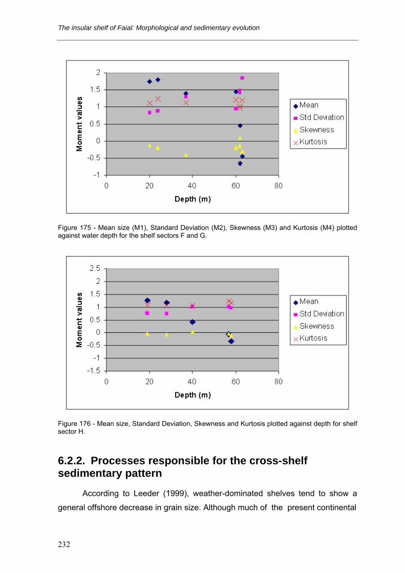
Figure 175 - Mean size (M1), Standard Deviation (M2), Skewness (M3) and Kurtosis (M4) plotted against water depth for the shelf sectors F and G.
Figure 176 - Mean size, Standard Deviation, Skewness and Kurtosis plotted against depth for shelf sector H.
6.2.2. Processes responsible for the cross-shelf sedimentary pattern
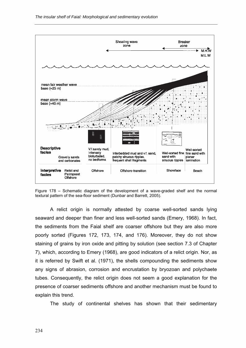
According to Leeder (1999), weather-dominated shelves tend to show a
general offshore decrease in grain size. Although much of the present continental
232

Chapter 6. Shelf sedimentary dynamics
Figure 177 – Carbonate percentages from the Faial shelf samples. The rocky outcrops correspond to the lava flows and coarse clastic deposits interpreted in Chapter 3.
shelf contains relict or palimpsest sediments (Emery, 1968; Swift et al., 1971),
those parts of the inner-shelf where sediment is accumulating today should show
such a seaward-fining profile (Figure 178), reflecting the balance between grain
size, water depth and wave energy (Dunbar and Barrett, 2005).
Surprisingly, being the Faial shelf a wave to storm-dominated system, the
sampling has shown the absence of this offshore-fining profile. On the contrary,
the data shows an offshore-coarsening profile, especially below 50 meters water
depth. The simplest explanation is to assume that at higher depths the presence of
relict or palimpsest sediments dominates. Relict sediments are sediments that
were deposited long time ago in equilibrium with their environments, most likely
when the sea level was lower than today. As the sea-level rose, the sedimentary
environments changed and the sediments are no longer in equilibrium (Emery,
1968). Therefore, the coarse sediments that are presently at greater depths could
have been formed in a shoreface environment that with the rise of sea-level has
changed to an outer shelf environment.
233
The insular shelf of Faial: Morphological and sedimentary evolution
Figure 178 – Schematic diagram of the development of a wave-graded shelf and the normal textural pattern of the sea-floor sediment (Dunbar and Barrett, 2005).
A relict origin is normally attested by coarse well-sorted sands lying
seaward and deeper than finer and less well-sorted sands (Emery, 1968). In fact,
the sediments from the Faial shelf are coarser offshore but they are also more
poorly sorted (Figures 172, 173, 174, and 176). Moreover, they do not show
staining of grains by iron oxide and pitting by solution (see section 7.3 of Chapter
7), which, according to Emery (1968), are good indicators of a relict origin. Nor, as
it is referred by Swift et al. (1971), the shells compounding the sediments show
any signs of abrasion, corrosion and encrustation by bryozoan and polychaete
tubes. Consequently, the relict origin does not seem a good explanation for the
presence of coarser sediments offshore and another mechanism must be found to
explain this trend.
The study of continental shelves has shown that their sedimentary
234

Chapter 6. Shelf sedimentary dynamics
sequences basically consist of beds displaying storm-induced depositional
structures intercalated with mud and shale layers. At short time scales, sediment
redistribution across the shelf is controlled by hydrodynamic processes, i.e. waves,
tides, geostrophic currents during storm events, whilst at longer time scales and 1-
100 m sequence scale the controlling factors are the accommodation space and
availability of sediments (Quiquerez et al., 2004). Several studies demonstrated
that winter storms are the agent causing much of the sediment dispersal on
coastal shelves. The effects of these storms are observable from shoreface to
water depths greater than 200m, at several tens of kilometres (Nittrouer and
Wright, 1994). Side-scan surveys after an intense winter storm at the Scotian shelf
showed the presence of hummocky megaripples in a region previously mapped as
featureless (Amos et al., 1996). These megaripples were linked to the storm,
which produced 7 m high significant waves. Box cores through the megaripples
revealed a well-defined tempestite bed 0.3 m thick overlying a lag layer of 4-cm
diameter pebbles (Amos et al., 1996). However, Lee et al. (1998) have shown that
these highly energetic events responsible for redistributing sediments to the shelf
have a very low recurrence. Conversely, fair-weather period is rather constant all
over the year and bioturbation and swell waves contribute significantly to the
smoothing of depositional profiles by favouring resuspension of the sediments
(Amos et al., 1996; Gagan et al., 1988). Lee et al. (1998) have also shown that it is
the interplay between the low recurrence groups of storm events and the steady
onshore feed of sediments from the shoreface during fair-weather conditions that
appear to play an important role on medium- and long-term profile evolution at
Duck beach, California. Furthermore, the onshore feeding of sediments in Duck
beach was not significantly affected by individual storms during the fair-weather
conditions, which lasted up to 4 years. On the contrary, the responsible for the
significant changes were the high energetic storm group events.
The mechanisms of which sediments are redistributed across the modern
shelves during the passage of storms are well established (Cookman and
Flemings, 2001). A range of wind stress orientations are present during the
passage of the storm and it can produce upwelling or downwelling (Figure 179B)
at different locations and at different times during a storm’s history. In the example
235

The insular shelf of Faial: Morphological and sedimentary evolution
of Figure 179A, shore-parallel wind stress drives a current at the sea surface
which is acted upon by the Coriolis force, causing the current to veer to the right.
This rotating flow adjacent to the water surface is called the surface Ekman layer
(Figure 179A) and the onshore component of the flow causes pilling of water on
the coast (coastal set-up). The resulting water surface gradient drives an offshore
current which extends throughout the entire water column and veers to the right,
producing a geostrophic flow oriented parallel to the shore. Below one Ekman
depth (D) is the geostrophic core where the interlayer shear stress goes to zero.
Near the sea floor, frictional forces retard the geostrophic flow, and the Coriolis
force causes the current to veer to the left. In this bottom Ekman layer, flow is
oriented obliquely offshore (Figure 179A).
It is clear that the Faial shelf is subjected to a very high energetic regime;
big storms struck the Azores (see section 2.2.4 of Chapter 2) and downwelling
currents were recorded associated to them (see section 2.4.4 of Chapter 2).
Therefore, four mechanisms often associated to storms could explain the
coarsening-offshore trend in the Faial shelf:
1. It is possible to assume that a very energetic event or group of events may
have swept off the shelf of Faial dispersing coarse sediments all over it. Strong
storm winds push surface waters landward and coastal setup results. The
resulting water surface gradient drives a downwelling offshore current which
transports sediments seaward. These extreme energetic events that affect the
entire shelf have probably a low frequency, much less than 1 per year. Only a
big storm could provoke downwelling currents strong enough to transport such
coarse sediments (coarse sands to granules) across the entire shelf. In fact, as
already discussed in section 2.2.4 of Chapter 2, violent storms occur once
every seven years. Nevertheless, it does not explain the transition between the
dominance of medium sands above 50 meters water depth to coarser
sediments below this depth (Figure 171).
2. Although most of the storm-bed models describe deposits which thin and
become more finely grained with increasing water depth and distance from
236

Chapter 6. Shelf sedimentary dynamics
shore due to offshore directed storm-surge ebb-flow, Gagan et al. (1990; 1988)
have shown that other patterns are also possible. They showed that
theWinifred storm-layer in the central Great Barrier Reef, Australia, becomes
thicker and more coarsely grained offshore. According to these authors, the
cross-shelf changes in thickness, texture and composition of the Winifred storm
bed were controlled by the changing response of a variable shelf substrate
rather than by shore-normal changes in the current velocity. Furthermore,
Figure 179 – A - In the northern hemisphere, downwelling (thick arrows show flow direction) results from steady wind oriented to right as observer faces seaward. Ekman layers develop at water surface and sea bed in response to boundary shear stresses. Geostrophic core has a constant shore-parallel velocity. B - Downwelling (D) occurs in deep and shallow regime if the wind is oriented (a) in quadrant III. Upwelling (U) occurs in deep and shallow regime if the wind is in quadrant I. If wind orientation is in quadrant II or IV, upwelling can occur in shallow zone and downwelling in deep zone (or vice versa) (Cookman and Flemings, 2001).
237

The insular shelf of Faial: Morphological and sedimentary evolution
resampling one year after showed preservation of the Winifred storm layer
nearshore and rapid reworking offshore below fair-weather wave-base. This
work shows that different shelf substrates may respond differently to storm
currents, resulting in storms beds that have significantly lateral variations in
thickness, texture and composition. However, the surface of the sand and
gravel deposits of the Faial shelf, except for the coarsening offshore pattern
and the varying calcium carbonate percentage, show a rather cross-shelf
uniform composition. The sediments are basically medium to coarse sands
composed of dark volcanic minerals and a variable percentage of skeletal
carbonate particles. The seismic interpretation also showed homogenous
sedimentary deposits. Although they present varied thickness, their geometry
and internal structure (see section 4.3.1 in Chapter 4) is the same all over the
shelf. Therefore, it would not be very convincing to explain the present-day
sedimentary pattern of the Faial shelf by the existence of a previous variable
shelf substrate.
3. As mentioned before, the downwelling currents directed offshore during storms
are known to be the major responsibles for the sediment redistribution in the
continental shelves. There might be however transport of sediments in any
direction, depending on the intensity, orientation (relative to the shoreline) and
duration of the storm winds. Probably unlikely, but possible, is to assume the
presence of strong winds blowing in the offshore direction resulting in the
predominance of upwelling currents that would transport finer sediments
onshore leaving the coarser offshore. In fact, the predominant wind directions
(higher frequencies and velocities) in the Faial Island (see section 2.3.1 in
Chapter 2) are those orientated towards S to SW and N to NE. The Coriolis
effect would cause net transport of surface and bottom waters approximately
directed W-E, which would only explain the fining landward trend in the shelf
sectors E and H (see Figure 169 for coastal orientation), leaving the
sedimentary pattern in the remaining sectors unexplained. Moreover, most of
the onshore transport of sand is attributed to wave asymmetry, whilst upwelling
currents are considered to be a process of secondary importance (Niedoroda
238

Chapter 6. Shelf sedimentary dynamics
et al., 1985).
4. Another possible explanation is to consider that the shelf break in Faial Island
is a zone of active sedimentation. The majority of the detailed surveys on the
outer margins have provided evidence of recent sediment displacement at and
near the shelf break (Southard and Stanley, 1976). Furthermore, there is also a
wide variety of data showing that relict sediment has been reworked since the
rise in sea level and continues to be modified at present resulting in palimpsest
sediment (Swift et al., 1971). Southard and Stanley (1976) reviewed the
physical processes at the shelf break capable of sediment entrainment and
transport at the shelf break. Several kinds of water movements seem to be
distinctive here. These distinctive processes when superimposed on bottom
currents caused by tides, waves and winds that are known to be typical of the
outer shelf environment, act to increase bottom sediment movements that
seem to be characteristic of the shelf edge. Tidal currents, especially on low-
latitude, gently sloping shelves, tend to be stronger on the outer shelf than
nearshore. Bottom currents produced by migration of the atmospheric
pressure-induced wave that migrates beneath a major storm moving in the
offshore direction can result in a current on the order of 10 cm/s concentrated
on the shelf break. Both theory and experiment suggest that internal waves of
tidal or shorter period propagating shoreward in thermoclines produce
intensified near-bottom velocities near the shelf edge as they steepen and
break. Large eddies generated at shear zones between major currents on the
shelf and in adjacent open-ocean should locally increase bottom velocities in
the shelf break region (Southard and Stanley, 1976). In conclusion, there seem
to be several processes that may be responsible for the winnowing of fine
sediments near the shelf break leaving behind the coarser fractions.
Furthermore, the shelf break in Faial Island occurs on average at depths that
vary between 55 and 80 meters (see Figure 57 in Chapter 3) which correspond
precisely to the range of depths where the coarser sediments dominate.
From what has been discussed above, it appears that the most likely
explanation of the offshore coarsening trend is the conjugation of two of the four
239
The insular shelf of Faial: Morphological and sedimentary evolution
mechanisms described. First, the existence of low recurrence and very energetic
events transport coarse sediments across the entire shelf of Faial through
downwelling currents. Then, transport of sediments at the shelf break (which was
mapped between 55 m and 80 m water depth – see Chapters 3 and 5) to the slope
provokes the winnowing of fine sediments between the 50 and 80 meters water
depth, causing the coarsening pattern found at these depths. Since the very
energetic events do not occur often (much less than one per year), the areas
below 50 meters water depth have not yet received sediments from the
downwelling currents. This would allow the outer shelf to be covered by sediments
with grain-size distribution similar to ones that are above 50 meters water depth,
homogenizing the entire sedimentary cover of the shelf.
6.3. Cross-shore sediment transport in the Faial
Island shelf
The seaward limit to significant sediment transport in sandy coastal regions
is of fundamental importance to understanding long and cross-shore sediment
budgets and modeling coastal evolution. The significance of the shoreface lies in
the role it plays in the exchange of sand with the continental shelf and whether the
offshore zone is a net source or a sink for beach sands (Cowell et al., 1999). The
shoreface (Figure 180) can be defined as the upper part of the continental shelf
that is affected by contemporary wave processes and extends from the limit of
wave run-up to the depth limit for wave-driven sediment transport (Cowell et al.,
1999).
The shoreface can be subdivided into an upper and lower section. The
upper shoreface, referred to as the littoral zone by Hallermeier (1981), is defined
as the region in which erosion and accretion result in significant (i.e. measurable)
changes in the beach profile during a typical year. The lower shoreface, referred to
as the shoal zone by Hallermeier (1981), experiences little sediment transport
processes under typical wave conditions, but significant morphological changes
can occur during extreme storm events.
The boundary between the upper and lower shoreface is referred to as the
240

Chapter 6. Shelf sedimentary dynamics
Figure 180 – Definition of the upper and lower shoreface profiles and the time scale of interest in the positioning of their limits (after Cowell et al., 1999).
depth of closure (or closure depth) and can be used to infer a seaward limit to
significant cross-shore sediment transport (Nicholls et al., 1998). According to
Hallermeier (1981), at the closure depth one should not expect vertical variations
higher than 0.3 m during a typical year. In the absence of repetitive submarine
beach profiles to determine the depth at which morphological change is
insignificant (less than 0.3 m), Hallermeier (1981) proposed that the depth of
closure dc could be predicted using the annual wave climate according to Equation
14:
2
2
568282sx
sxsxc gT
H.H.d −= (14)
Where Hsx is the nearshore significant wave height that is exceeded only 12
hours each year (e.g. one should look in the data for the highest waves of the
record that occur with this frequency: 12h/(365days×24h)×100%=0.137%), Tsx is
the associated wave period and g the acceleration due to gravity. Equation 14 was
generalized to a time-dependent form by Stive et al. (Equation 15, 1992):
2
2
568282e,t
e,te,tl,t gT
H.H.d −= (15)
241

The insular shelf of Faial: Morphological and sedimentary evolution
Where: dl,t is the dc over t years; He,t is the significant non-breaking wave
height that is exceeded 12 hours per t years, (0.137/t)% of the time; Te,t is the
associated wave period and g the acceleration due to gravity.
It has been shown in several studies that the predictive equations for the dc
(Equations 14 Equation 15) provide good estimations although they use simple
wave parameters (Hallermeier, 1981; Nicholls et al., 1998). However, these
studies have also revealed uncertainties in this estimation, which allows for the
following considerations (Capobianco et al., 2002; Cowell et al., 1999):
• The depth of closure is time and space-scale dependent and generally the
lateral (shore-normal) migration of the theoretical closure depth increases with
time-scale (Figure 181a). The stretching of the theoretical closure depth also
involves seaward shift of this limit during storms (Figure 181b) and landward
shift during fair-weather conditions.
Figure 181 – Movements in the seaward boundary of the closure depth: (a) at intervals significantly longer than the annual time scale; (b) seaward displacement of the closure depth due to a severe storm with a return interval greater than 1 year. (Cowell et al., 1999).
• The depth of closure is a morphodynamic boundary, not a sediment transport
boundary. Sediment transport occurs seaward of the closure depth, especially
during storms. However, the closure depth is a good empirical indicator of an
increasing capacity for shoreward sediment transport at any point within the
limits of closure.
242

Chapter 6. Shelf sedimentary dynamics
• At small scales, the depth of closure is usually the product of bar migration due
to surf zone processes (Nicholls et al., 1998). As the scale increases, so does
beach-nearshore profile translation and ultimately shoreface processes come
to control the location of closure.
• In two-dimensional situations, the analytical formulation for dc (Hallermeier,
1981) provides robust estimates of the limit of closure for individual erosional
events up to the annual time-scale (Nicholls et al., 1998). Between annual and
decadal scales, it continues to act as a limit, but with an increasing tendency
for overprediction. The dc only considers cross-shore redistribution of sediment
and is invalid in areas which are accreting rapidly due to longshore supply of
sand.
6.3.1. Estimation of the seaward limit of the upper shoreface
The wave-climate data (Carvalho, 2003) used to estimate the seaward limit
of the upper shoreface (closure depth - dc) includes the annual average hindcast of
Hs(m0) and the Tp for the period of 1989-2002 (Tables 1 and 2 in Chapter 2). As
already discussed in the section 2.2.3 of Chapter 2, there is the need to use in the
calculations the Hs and Ts; therefore, the Equations 3, 4, 5 and 8 (see Chapter 2)
are used to convert Hs(m0) into Hs and Tp into Ts. Since the hindcast data provides a
period bigger than one year, it is possible to use the Equation 15 from Stive et al.
(1992) to estimate the dc for a 14 year period. Including an enlarged period is
important, because it will take into account more energetic events although there
is the risk of overestimation for the dc. Nevertheless, overestimation can be a safer
approach when it comes to decide at which depth aggregates can be explored
without putting at risk the coastline (see Chapter 7). Therefore, the dc is calculated
for each coastal sector, using the values of Hs and Ts that are exceeded only 12
hours during the 14 years period (which are referred respectively as He,t and Te,t in
the Equation 15). For instance, to calculate the NE Hs that is exceeded only 12
hours during the 14 years period – (0.137/14)% of the time - one should look for
the highest waves in the record that have a frequency of 0.00978% (e.g. in Table 1
243

The insular shelf of Faial: Morphological and sedimentary evolution
the NE Hs(m0) must result from a linear interpolation between 7 m (0.020%) and 8
m (0%), which gives 7.51 m and since Hs = Hs(m0), the value is the same – see
Table 15). To calculate the NE Ts that is exceeded only 12 hours during the 14
years period – (0.137/14)% of the time - one should look for the highest periods in
the record that have a frequency of 0.00978% (e.g. in Table 2 the NE Tp must
result from a linear interpolation between 14 s (0.015%) and 15 s (0%), which
gives 14.51 s and using Equations 4, 5, and 8 the value 11.97s is found – see
Table 15).
The closure depth estimated with Equation 15 (Table 15) gives values
between 10 m (coastal sector perpendicular to the SE direction) to 26 m (coastal
sector perpendicular to the W direction). In reality, this kind of analysis only makes
sense for coastal sectors that have nearshore sands and these are only present in
the coastal sectors B, E and H (see sectors orientation in Figure 169). Therefore,
in a typical year, sectors B, E and H should not have vertical variations higher than
0.3 m below the respective water depths of 24 m, 11 m and 20 m.
Table 15 - Estimation of closure depth based on Equation 15. The represented quadrants are relative to wave ray directions.
He,t (m) Te,t
* (s) dl,t
* (m)
NE 7.510 11.973 14.373
E 5.840 10.304 11.070
SE 5.350 9.862 10.141
S 5.960 10.029 11.120
SW 11.040 12.808 19.978
W 13.720 15.669 25.923
NW 12.040 16.445 23.705
N 8.510 13.901 16.783
The transition from the upper to the lower shoreface is generally not
characterized by a change in morphology. However, the theoretical closure depth
may correspond to a distinct break in sediment characteristics (Niedoroda et al.,
1985). Upper shoreface sands are usually well-sorted and similar to beach
244

Chapter 6. Shelf sedimentary dynamics
sediments, and tend to display a seaward-fining trend. In many places, the
seaward fining of sediments occurs down to an abrupt transition at a depth similar
to dc, seaward of which coarser, poorly sorted sand may be found. In this work, a
detailed sampling is not available (samples were always taken below 20 m water
depth) to check if the transition from the upper to the lower shoreface shows such
a change in the sediment characteristics.
6.3.2. Estimation of the seaward limit of the lower shoreface
As mentioned before, the lower shoreface does not suffer significant vertical
changes (less than 0.3 m) in a typical year. Furthermore, its seaward limit
represents the depth of sediment immobility during a normal year. Only during
extreme storm events, significant changes can occur in the lower shoreface and
sediments can be transported beyond the seaward limit of it. Because the seaward
limit of the lower shoreface depends greatly on the time scale of interest (Figure
180), it is less straightforward to define. However, in the absence of other clear-cut
definitions, it is useful to turn to another of Hallermeier’s (1981) criteria for
estimating this limit (Cowell et al., 1999). Based on a synthesis of theoretical and
field studies, Hallermeier (1981) estimated that the limiting depth for the on-
offshore transport of sand by waves throughout a typical year is given by:
(16) 1 2500 3 5000 /
i s s sd (H . σH )T (g / D )= −
Where Hs is the nearshore annual average significant wave height; σHs is
the standard deviation of Hs, Ts is the associated wave period, g the acceleration
due to gravity and D50 is the size of the median sediment (in meters) determined
from a sand sample taken in a water depth (h) of h=1.5 dc. The Hs for each
quadrant (corresponds to Hsav in Chapter 2) is calculated from Table 1 in Chapter 2
using Equation 9. To calculate the standard deviation of the Hs per quadrant (σHs),
first one must calculate each monthly average significant wave height per
quadrant, using also Equation 9. This is possible because Carvalho (2003)
245

The insular shelf of Faial: Morphological and sedimentary evolution
provides tables similar to Table 1 but with monthly average significant wave
heights (these are averages from January to December for the 14 year period -
1989-2002). Then, the values of each monthly average significant wave height per
quadrant are used to calculate the annual standard deviation of Hs. The median
size used in the calculations was derived from the nearest sample of the required
water depth h, since very often there were no samples at this water depth. The Ts
for each quadrant (corresponds to in Chapter 2) is calculated from Table 2 in
Chapter 2 using the Equation 10 and then Equations 4, 5 and 8.
pavT
Table 16 shows the estimations for the seaward limit of the lower shoreface
where these vary between 29 and 49 meters water depth. In this case, the
differences are primary related with the annual variation of the value of Hs for the
distinct directional sectors.
Table 16 - Estimation of the offshore limit of the lower shoreface based on the Equation 16. The represented quadrants are relative to wave ray directions.
Hs (m) Ts(m) σ Hs D50 (m) h=1.5 dc (m) di (m) NE 1.870 7.197 0.678 0.000342 20.930 28.730 E 1.913 6.665 0.599 0.000242 16.090 32.850
SE 2.211 6.685 0.598 0.000261 14.740 37.238 S 2.456 7.037 0.576 0.000295 16.120 41.403
SW 2.999 7.777 0.893 0.000403 28.780 46.817 W 2.964 8.609 1.034 0.000426 37.660 48.984
NW 2.480 8.463 0.944 0.000438 34.700 39.316 N 2.018 7.580 0.779 0.000342 24.570 32.407
However, one question remains. How representative was the grain
diameter used for the calculations, considering the variable nature of the sediment
distribution on the lower shoreface? A simple alternative approach to defining the
seaward limit of the lower shoreface is through the application of the wave base
concept, where wave base is defined as water depth beyond which wave actions
ceases to stir the sediments bed (Cowell et al., 1999). Conventionally, this limit is
taken to be where the water depth (hLS) is half the deep-water wave length (L0) -
Equation 17 - which corresponds to the deep-water transition to intermediate-
246

Chapter 6. Shelf sedimentary dynamics
water waves.
hLS=L0/2 (17)
The general expression for wave length according to linear Airy wave
theory is (Dean and Dalrymple, 1991):
⎟⎠⎞
⎜⎝⎛=
Lπ
πgTL 2tanh2
2
(18)
And for the special case of deep-water waves, , so that
wave length simply becomes:
tanh(2 / L) 1→π
(19) π/gTL 220 =
Where L0 is the deep-water wave-length, T the period and g the
acceleration due to gravity (9.81 m/s2). For this case it will also be used the of
Chapter 2 and then use the Equations 4, 5 and 8.
pavT
The seaward limit of the lower shoreface (Table 17) calculated with this
method is very similar for some sectors, whilst for others it shows some significant
differences (e.g. 16.6 m difference for waves coming from NW). Nevertheless,
both methods put more or less this limit between 30 and 50 m, depending
essentially on the values of the wave height and period for Equation 16 and period
for Equation 17.
Figure 182 shows theoretical curves based on the Equation 16 for all wave
directions and grain size distributions. The curves were drawn with the values of Hs
and Ts for each quadrant (Table 16) and using increasing theoretical values of D50.
If one looks to the curve generated by the southwestern waves (sector H), the
area above the dark red curve represents all the sediments that at the respective
depths and grain size do not suffer transport in a typical year; they are only
247

The insular shelf of Faial: Morphological and sedimentary evolution
Table 17 - Estimation of the offshore limit of the lower shoreface based on of the wave base concept using Equation 17. The represented quadrants are relative to wave rays directions.
L0 (m) T (s) hLS (m)
NE 80.797 7.197 40.399
E 69.292 6.665 34.646
SE 69.712 6.685 34.856
S 77.243 7.037 38.621
SW 94.329 7.777 47.165
W 115.597 8.609 57.798
NW 111.721 8.463 55.861
N 89.619 7.580 44.809
transported during extreme storms events. The area below the curve represents
all the sediments that the respective depths and grain size, suffer transport,
although by definition the transport in the lower shoreface is not very significant in
terms of quantity. If one looks to the graphic of the Figure 171, it is obvious that
the sediments are coarser below 50 meters water depth. And if one plots those
sediments in a graph (Figure 183) like the one of the Figure 182 it is also obvious
that the shelf sediments below 30 m water depth do not suffer transport for the
lower energy wave quadrant (sector E) and even for the second higher energy
wave quadrant (sector H), all the samples below 50 m water depth are immobile.
Therefore, in a typical year, depending on the shelf sectors, below 30 meters
water depth (e.g. sector E) or 50 meters water depth (e.g. sector H), the respective
sector shelf sediments are immobile. One tends immediately to find a parallelism
between the offshore limit of the lower shoreface in the more energetic sectors
and the distinct change in the characteristics of sediments below 50 meters water
(Figure 171 and Figure 183). It appears that the offshore limit of the lower
shoreface for the second higher energetic shelf sector (sector H, di = -46.8 m)
roughly coincides with the coarsening trend below 50 meters water depth. This
evidence supports the hypothesis discussed in the section 6.2.2, that only during
extreme storm events the shelf below 50 meters water depth is affected by the
248

Chapter 6. Shelf sedimentary dynamics
transport of sediments. Otherwise, the sedimentary cover would be homogenized
every year and the grain-size distribution would also be the same all over the
shelf.
Figure 182 – Theoretical curves for all wave quadrants based on Equation 16 using the values of Hs and Ts for each quadrant expressed in Table 16 and increasing values of D50.
Figure 183 - Theoretical curves for the second higher and the lower energy wave quadrants (respectively SW and E) based on Equation 16 and the Faial shelf samples plotted.
From what as been discussed above, it seems that the shoreface in the
Faial Island extends down to 50 meters water depth, which is, in some shelf
sectors, almost the entire shelf area. Therefore, it does not make sense to
individualize the shoreface from the rest of the shelf like it is shown in Figure 180.
249

The insular shelf of Faial: Morphological and sedimentary evolution
6.3.3. Estimation of sediment entrainment depth during storm events
The offshore limit of the lower shoreface is not a guarantee of sediment
immobility, since during extreme storms, sediment transport can occur well beyond
this limit. It would be interesting to have a notion of how deep can storms (for
instance the storm which wave height is exceeded only 12 hours in 14 years)
affect sediment mobility. This wave height was chosen because the aim is to
calculate the entrainment depth for low occurrence and high energetic storms. In
order to get an accurate value for it, it was decided to use the approach of the
grain settling velocity to predict the entrainment threshold of sediments on a plane
bed by oscillatory waves. For that purpose it is necessary to calculate the critical
wave orbital velocity (Uwc). The Uwc can be determined from the equations of Le
Roux (Le Roux, 2001; Le Roux, 2005):
( ) 31250
/yd /μρgρDD = (20)
for 2.9074 < D( 37002360 .D.W ddv −= )
)
d < 22.9866 (21)
for 22.9866 < D( 3245082550 /ddv .D.W −= d < 134.9215 (22)
(23) 55002460 .-dvdwc W.U =
( ) ( ) ( ) ( )2 0 550 500 01 1 3416 0 6485.
wc dwc y dwc yU . U gD ρ / ρμ / T . U gD ρ / ρ / T .μ⎡ ⎤ ⎡ ⎤= − + −⎢ ⎥ ⎣ ⎦⎣ ⎦
for < 50 cm/s (24) wcU
for wcU up to 150 cm/s (25) 675700270 .-dvdwc W.U =
250
Chapter 6. Shelf sedimentary dynamics
( )0 52 2 2 250 500 002 1 0702 .
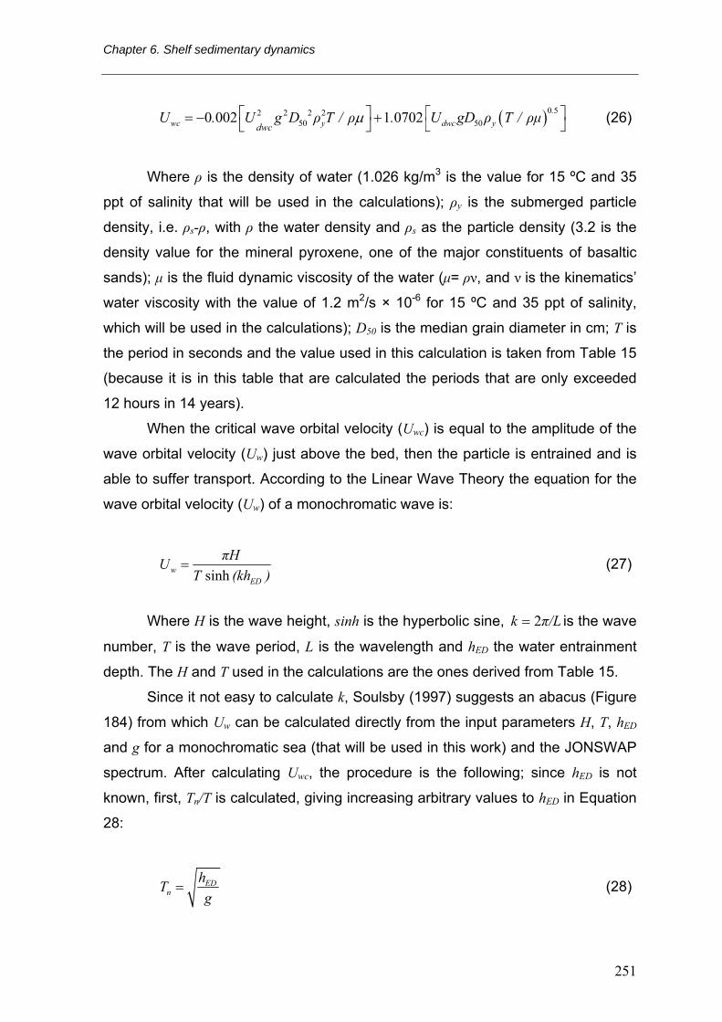
wc y dwc ydwcU . U g D ρ T / ρ . U gD ρ T / ρμμ⎡ ⎤ ⎡ ⎤= − + ⎣ ⎦⎣ ⎦ (26)
Where ρ is the density of water (1.026 kg/m3 is the value for 15 ºC and 35
ppt of salinity that will be used in the calculations); ρy is the submerged particle
density, i.e. ρs-ρ, with ρ the water density and ρs as the particle density (3.2 is the
density value for the mineral pyroxene, one of the major constituents of basaltic
sands); μ is the fluid dynamic viscosity of the water (μ= ρν, and ν is the kinematics’
water viscosity with the value of 1.2 m2/s × 10-6 for 15 ºC and 35 ppt of salinity,
which will be used in the calculations); D50 is the median grain diameter in cm; T is
the period in seconds and the value used in this calculation is taken from Table 15
(because it is in this table that are calculated the periods that are only exceeded
12 hours in 14 years).
When the critical wave orbital velocity (Uwc) is equal to the amplitude of the
wave orbital velocity (Uw) just above the bed, then the particle is entrained and is
able to suffer transport. According to the Linear Wave Theory the equation for the
wave orbital velocity (Uw) of a monochromatic wave is:
sinhw
ED
πHUT (kh )
= (27)
Where H is the wave height, sinh is the hyperbolic sine, is the wave
number, T is the wave period, L is the wavelength and h
π/Lk 2=
ED the water entrainment
depth. The H and T used in the calculations are the ones derived from Table 15.
Since it not easy to calculate k, Soulsby (1997) suggests an abacus (Figure
184) from which Uw can be calculated directly from the input parameters H, T, hED
and g for a monochromatic sea (that will be used in this work) and the JONSWAP
spectrum. After calculating Uwc, the procedure is the following; since hED is not
known, first, Tn/T is calculated, giving increasing arbitrary values to hED in Equation
28:
EDn
hTg
= (28)
251

The insular shelf of Faial: Morphological and sedimentary evolution
Then, using the graph of the Figure 184, the value of Uw×Tn/2H (y-axis) for
a monochromatic sea is taken after the value of Tn/T (x-axis); next assuming for
instance that Uw×Tn/2H = 0.2, Uw can be calculated with the following formulae:
Uw = 0.2×2H/Tn (29)
Or, generalizing:
Uw = Y×2H/Tn (30)
This procedure is repeated giving increasing values to hED in Equation 28
until Uwc is found to be equal to Uw (Equation 30) and the final value of hED is
found.
Figure 184 – Abacus for determining Uw for monochromatic waves (this case) using the input parameters UwTn/2H and Tn /T (from Soulsby, 1997). Uw is determined with the following relationship
with Y as the value taken from the curve in the vertical axis. YH/TU nw ×= 2
The grain-size of the sediments chosen, were derived from the natural
variability found on the shelf. It was chosen the median diameter (D50) of the finer,
middle and coarser sediment to cover the complete size distribution of the set of
samples.
The results from Table 18 show that the storms (coming from NW) which Hs
252
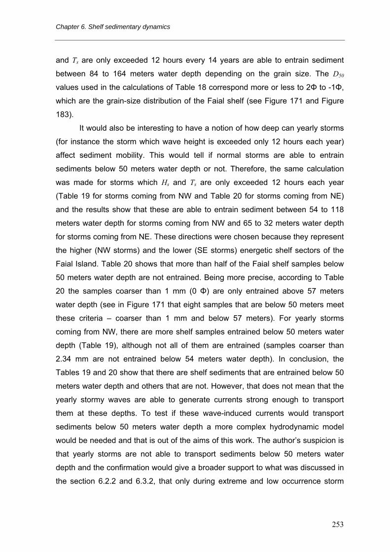
Chapter 6. Shelf sedimentary dynamics
and Ts are only exceeded 12 hours every 14 years are able to entrain sediment
between 84 to 164 meters water depth depending on the grain size. The D50
values used in the calculations of Table 18 correspond more or less to 2Φ to -1Φ,
which are the grain-size distribution of the Faial shelf (see Figure 171 and Figure
183).
It would also be interesting to have a notion of how deep can yearly storms
(for instance the storm which wave height is exceeded only 12 hours each year)
affect sediment mobility. This would tell if normal storms are able to entrain
sediments below 50 meters water depth or not. Therefore, the same calculation
was made for storms which Hs and Ts are only exceeded 12 hours each year
(Table 19 for storms coming from NW and Table 20 for storms coming from NE)
and the results show that these are able to entrain sediment between 54 to 118
meters water depth for storms coming from NW and 65 to 32 meters water depth
for storms coming from NE. These directions were chosen because they represent
the higher (NW storms) and the lower (SE storms) energetic shelf sectors of the
Faial Island. Table 20 shows that more than half of the Faial shelf samples below
50 meters water depth are not entrained. Being more precise, according to Table
20 the samples coarser than 1 mm (0 Φ) are only entrained above 57 meters
water depth (see in Figure 171 that eight samples that are below 50 meters meet
these criteria – coarser than 1 mm and below 57 meters). For yearly storms
coming from NW, there are more shelf samples entrained below 50 meters water
depth (Table 19), although not all of them are entrained (samples coarser than
2.34 mm are not entrained below 54 meters water depth). In conclusion, the
Tables 19 and 20 show that there are shelf sediments that are entrained below 50
meters water depth and others that are not. However, that does not mean that the
yearly stormy waves are able to generate currents strong enough to transport
them at these depths. To test if these wave-induced currents would transport
sediments below 50 meters water depth a more complex hydrodynamic model
would be needed and that is out of the aims of this work. The author’s suspicion is
that yearly storms are not able to transport sediments below 50 meters water
depth and the confirmation would give a broader support to what was discussed in
the section 6.2.2 and 6.3.2, that only during extreme and low occurrence storm
253
The insular shelf of Faial: Morphological and sedimentary evolution
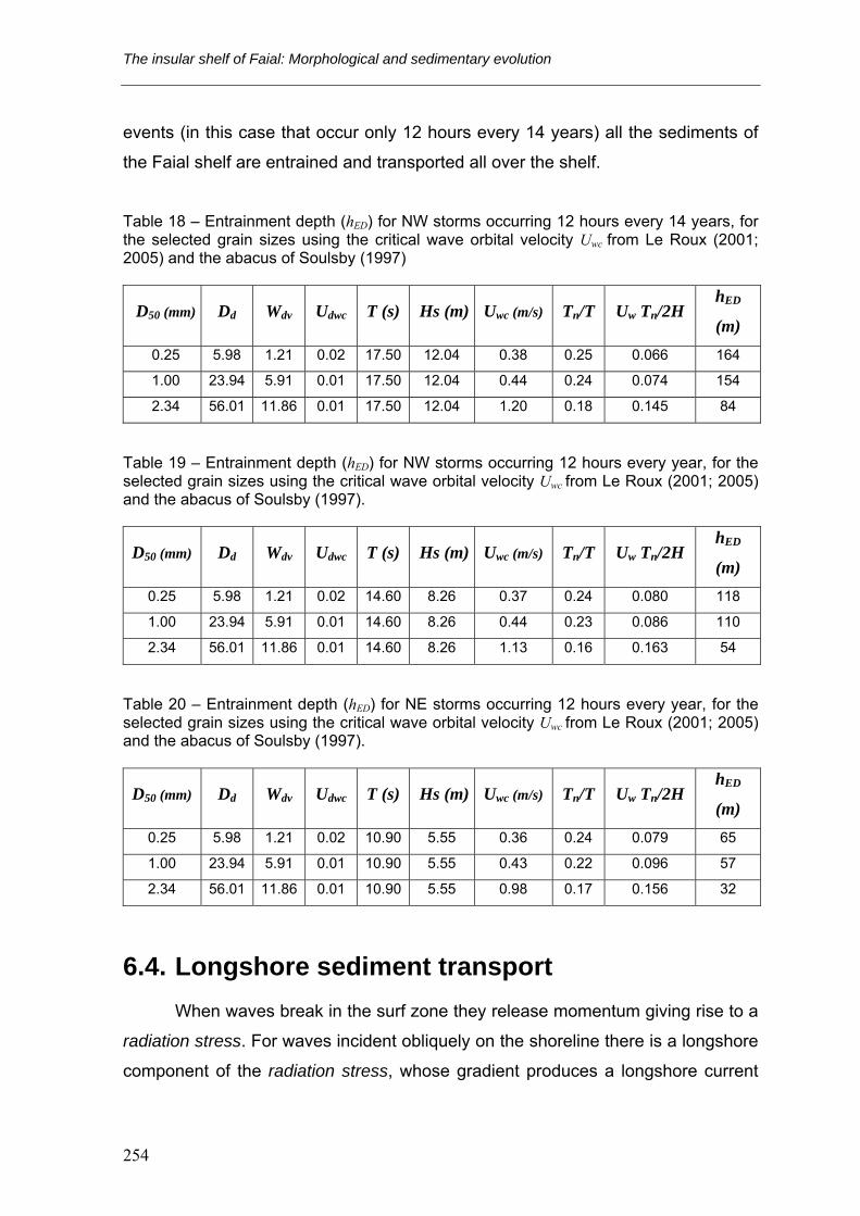
events (in this case that occur only 12 hours every 14 years) all the sediments of
the Faial shelf are entrained and transported all over the shelf.
Table 18 – Entrainment depth (hED) for NW storms occurring 12 hours every 14 years, for the selected grain sizes using the critical wave orbital velocity Uwc from Le Roux (2001; 2005) and the abacus of Soulsby (1997)
D50 (mm) Dd Wdv Udwc T (s) Hs (m) Uwc (m/s) Tn/T Uw Tn/2H hED
(m) 0.25 5.98 1.21 0.02 17.50 12.04 0.38 0.25 0.066 164
1.00 23.94 5.91 0.01 17.50 12.04 0.44 0.24 0.074 154
2.34 56.01 11.86 0.01 17.50 12.04 1.20 0.18 0.145 84
Table 19 – Entrainment depth (hED) for NW storms occurring 12 hours every year, for the selected grain sizes using the critical wave orbital velocity Uwc from Le Roux (2001; 2005) and the abacus of Soulsby (1997).
D50 (mm) Dd Wdv Udwc T (s) Hs (m) Uwc (m/s) Tn/T Uw Tn/2H hED
(m) 0.25 5.98 1.21 0.02 14.60 8.26 0.37 0.24 0.080 118
1.00 23.94 5.91 0.01 14.60 8.26 0.44 0.23 0.086 110
2.34 56.01 11.86 0.01 14.60 8.26 1.13 0.16 0.163 54
Table 20 – Entrainment depth (hED) for NE storms occurring 12 hours every year, for the selected grain sizes using the critical wave orbital velocity Uwc from Le Roux (2001; 2005) and the abacus of Soulsby (1997).
D50 (mm) Dd Wdv Udwc T (s) Hs (m) Uwc (m/s) Tn/T Uw Tn/2H hED
(m) 0.25 5.98 1.21 0.02 10.90 5.55 0.36 0.24 0.079 65
1.00 23.94 5.91 0.01 10.90 5.55 0.43 0.22 0.096 57
2.34 56.01 11.86 0.01 10.90 5.55 0.98 0.17 0.156 32
6.4. Longshore sediment transport
When waves break in the surf zone they release momentum giving rise to a
radiation stress. For waves incident obliquely on the shoreline there is a longshore
component of the radiation stress, whose gradient produces a longshore current
254

Chapter 6. Shelf sedimentary dynamics
within (and just outside) the surf zone which is balanced by friction within the bed
(Soulsby, 1997). This in turn drives sediment along-shore as a littoral drift. The
longshore sediment transport rate (QLS) measures the littoral drift across an area
normal to the shoreline. Variations in QLS along the shoreline cause recession or
advance of the shoreline in question. The CERC formula (Coastal Engineering
Research Centre, 1984) is the most widely used method to calculate the total
sediment transport QLS integrated across the width of the surf zone. However, it
does not include dependencies on grain size, beach slope and wave period and,
although it proves valuable for the transport of sediments by suspension, for grain
sizes bigger than 0.5 mm it has a tendency for overestimation (Soulsby, 1997).
Damgaard and Soulsby (1997) proposed a formula for bedload longshore
sediment transport which has probably a better applicability for Faial shorefaces.
The reason is that most of the samples taken on the shelf revealed sediments
coarser than 0.5 mm, which means that the transport mechanism will be manly
beadload instead of suspension. The resulting formula is:
QLS = maximum of QLS1, QLS2a and QLS2b (31)
( ) ( ) ( )
( )112
ˆ12sintan19.0 2/52/32/1
1 −−
=s
HgQ crbb
LSθαβ
for < 1 (32) crθ̂
for 1 (33) 01 =LSQ ≥crθ̂
( )
3/8 1/4 19/850
2 1/4
0.24 ( )12 1
b bLS a
f g D HQs T
α=
− for wsfwr θθ ≥ (34)
( )
2/5 13/5
2 6/5 1/5
0.046 ( )12 1 ( )
b bLS b
f g HQs T
απ
=−
for wsfwr θθ < (35)
for cr02 =LSQ θθ <max (36)
Where:
255
The insular shelf of Faial: Morphological and sedimentary evolution
( ) 5016.7 1ˆ
(sin 2 )(tan )cr
crb b
s DH
θθ
α β−
= (37)
)2)(sin2cos19.095.0()( bbbf ααα −= (38)
( )
3/4
1/4 1/250
0.151 ( )
bwr
Hs g TD
θ =−
(39)
( )
6/5
7/5 1/5 2/550
0.0041
bwsf
Hs g T D
θ =−
(40)
wθ = maximum of wrθ and wsfθ (41)
( ) 50
0.1 (sin )(tan )1
b bm
Hs D
α βθ =−
(42)
(43) ( ) ([ 2/122max cossin bwbwm αθαθθθ ++= ) ]
[ )02.0exp(1055.02.113.0
dd
cr DD
−−++
=θ ] (44)
2/sbb HH = (45)
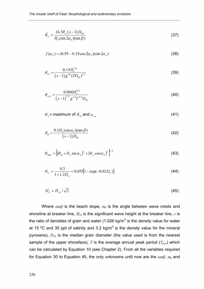
Where tanβ is the beach slope, αb is the angle between wave crests and
shoreline at breaker line, Hsb is the significant wave height at the breaker line, s is
the ratio of densities of grain and water (1.026 kg/m3 is the density value for water
at 15 ºC and 35 ppt of salinity and 3.2 kg/m3 is the density value for the mineral
pyroxene), D50 is the median grain diameter (the value used is from the nearest
sample of the upper shoreface), T is the average annual peak period (Tpav) which
can be calculated by Equation 10 (see Chapter 2). From all the variables required
for Equation 30 to Equation 45, the only unknowns until now are the tanβ, αb and
256

Chapter 6. Shelf sedimentary dynamics
Hb.
The beach slope (tanβ) was calculated using the definition of closure depth.
The slope was calculated for the upper shoreface using as the inshore limit the
coastline and the offshore limit the closure depth estimated in Table 15. Therefore,
upper shoreface profiles were made for each shelf sector using the bathymetric
data of Figure 56 in Chapter 3 to calculate the distance between the coastline and
the closure depth. More complex to calculate are the values of αb and Hb. For that
purpose, the methodology suggested in the exercise II-1-1 from the U.S. Army
Corp of Engineers (2003b) and exercise II-3-1 from the U.S. Army Corp of
Engineers (2003a) was used. First, the deep-water wavelength (L0) was calculated
using Equation 19:
Then, the intermediate water wavelength (L) was calculated:
⎟⎠⎞
⎜⎝⎛=
LdgTL bπ
π2
tanh2
2
(46)
With db being the water depth at breaker line. Since db is not yet known, the
value of 2m will be used in the beginning of the calculations. The use of Equation
46, involves however some difficulty since the unknown L appears on both sides of
the equation. Since db/L0 is known, the following relationship (Equation 47) is used
to estimate db/L by trial and error (for instance if d/L0 = 0.5, random values of L will
be given until the right hand-side of Equation 47 reach 0.5 or the nearest value
with an approximation of 5 decimals and finally L is found).
0
2tanh ⎛= ⎜⎝ ⎠
b b bd d dL L L
π ⎞⎟ (47)
Once L and L0 are calculated it is possible determine the shoaling
coefficient Ks:
2/1
0
⎟⎟⎠
⎞⎜⎜⎝
⎛=
g
gs C
CK (48)
257

The insular shelf of Faial: Morphological and sedimentary evolution
00 21 CCg = (49)
(50) TC 56.10 =
⎟⎠⎞
⎜⎝⎛
⎟⎟⎠
⎞⎜⎜⎝
⎛+=
LdgT
LdLd
C b
b
bg
πππ
π 2tanh
2)/4sinh(/4
121 (51)
Where Cg0 is the deep-water wave group velocity, C0 is the deep-water
wave speed and Cg is the intermediate-water group velocity. Then the angle αb can
be determined by the following relationship (Equation 52):
0
0sinsinCC
b αα= (52)
TLC = (53)
Where C is the shallow-water wave speed and α0 is the deep-water angle
between wave crests and depth contours. Once sin αb is known it is possible to
calculate the refraction coefficient (Kr):
41
20
2
sin1sin1
⎟⎟⎠
⎞⎜⎜⎝
⎛−−
=b
rKαα (54)
Finally, the significant wave breaker height (Hsb) can be determined with the
following equation:
(55) Sb s rH HK K=
Where H is the mean annual significant deep-water wave height and was
258
Chapter 6. Shelf sedimentary dynamics
estimated using Equation 9 from Chapter 2. Now, it is possible to estimate the
breaker depth (db) with the Equation 56 taken from Dean and Dalrymple (1991)
after Weggel (1972):
(56) bSb dkH ′=
2gTH
abk b−=′ (57)
( )βtan1918.43 −−×= ea (58)
( ) 1tan5.19156.1 −−×= βeb (59)
The value of the breaker depth (db) calculated using Equation 56 is checked
against the value initially estimated to be used in Equation 47 (2m). If different, the
value just determined is substituted in Equation 45 and this procedure will be
repeated until one gets a difference smaller than 0.009 between the db calculated
with Equation 56 and the db from the previous run. The longshore sediment
transport was calculated only for the sectors B (with an average coastal orientation
of 40º) and H (with an average coastal orientation of 165º), since these have
nearshore sediments able to suffer transport in the surf zone. They also have
bathymetric contours relatively parallel to the shore, which would not introduce
significant errors in the calculation of the refraction coefficient (Kr), the angle (αb)
between wave crests and shoreline at breaker line, the wave breaker height (Hsb)
and the breaker depth (db). The complex bathymetry of the channel Faial-Pico and
the sheltering effect of Pico Island would introduce significant errors in the
calculation of the longshore drift in sector E and for that reason it was not
estimated.
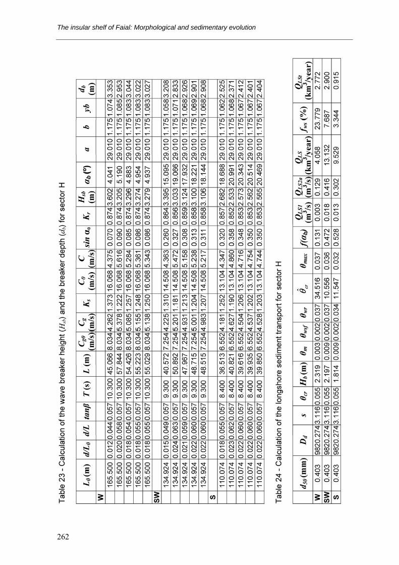
Table 21 shows the calculation of the wave breaker height (Hsb) and the
breaker depth (db) for sector B and Table 23 the same calculation for sector H.
Table 22 shows the calculation of the longshore sediment transport for sector B
259

The insular shelf of Faial: Morphological and sedimentary evolution
where it was used the waves from W, N and NW and Table 24 shows the same
calculation for sector H where it was used the waves from W, S and SW. The
longshore sediment transport (QLS) that appears in Tables 22 and 24 was
calculated assuming that all wave directions have the same frequency, which is
not the case. Therefore the real longshore sediment transport (QLSt) was calculated
considering the annual wave frequency of each wave direction (fws in Tables 22
and 24).
The net longshore drift for sector B is 1.478 km3 per year in the NE
direction. Although the NE waves apparently do not contribute to the longshore
transport in the sector B (due to its costal orientation) if they suffer refraction, they
could eventually invert the transport to the SW direction. The net longshore drift for
sector H is 0.363 km3 per year in the NW direction. The direction of the longshore
transport in sector B and H should be taken into account when decisions regarding
the dredging licensing will be decided. For instance, the SE part of sector H does
not have beaches, but dredging too near the shore may put in risk the beach of
Varadouro (in the NW part of this sector) since the net transport in this sector is in
the NW direction.
Although in the other shelf sectors there could not be longshore transport
due to lack of sand and gravels nearshore, during extreme storm events wave-
induced currents might affect the sea-floor at depths where the bottom is covered
by sand and gravels. In the Figure 185 the annual average wave regime and the
respective affected coastal sectors are drawn. A brief analysis of the data permits
to infer which would be the net transport directions based on the annual frequency
and annual average heights of the set of waves that affect each costal sector.
Figure 186 represents the longshore transport of sediment that occurs mostly
during extreme storm events. The few exceptions are the shelf sectors B, E and H
which transport can occur all over the year, because they have sand and gravels
nearshore. The bold black lines represent the barriers to sediment transport
across different shelf sectors. Therefore, for shelf sectors A1, A2, C+D, E, F+G the
net longshore transport would be respectively, SE, E, SSE, S and E, because the
higher and more frequent waves would probably transport sediments in these
directions (Figures 185 and 186). During these extreme storm events there is also
260

Chapter 6. Shelf sedimentary dynamics
261
The insular shelf of Faial: Morphological and sedimentary evolution
262

Chapter 6. Shelf sedimentary dynamics
the possibility of sediments crossing more than one shelf sector. The less likely
passages would be (Figure 186):
Figure 185 – Annual average wave regime showing wave frequency and wave height affecting the respective shelf sectors. The arrows represent the wave directions that affect each shelf sector.The bold colored lines around the coast of Faial and the black capital letters represent the different shelf sectors.
1. From H to G, because net transport of sediments is on opposite directions for
each sector. In addition there are coarse clastic deposits in the intersection of
these two sectors that represent bathymetric highs that would stop the
sediment passage.
2. From B to C, because there are coarse clastic deposits at the intersection of
these two sectors that represent bathymetric highs that would stop the
sediment passage.
3. From F to E, because there is a bathymetric embayment in front of Monte da
Guia that would act as a sink for sediments trying to cross (see Figure 56 in
Chapter 3).
263

The insular shelf of Faial: Morphological and sedimentary evolution
The likely passages (Figure 186) would be from A2 to B, from A1 to H, from
C to D, From G to F and eventually from D to E, because there are no evident
obstacles impeding the passage. The only one more dubious is the passage from
D to E, because there are coarse clastic deposits nearshore up to 50 meters water
depth that would prevent sediments crossing above this depth.
Figure 186 – Net longshore drift on the shelf sectors represented by the arrows. The bold black lines represent shelf features that are barriers to sediment transport. The bold colored lines around the coast of Faial and the black capital letters represent the different shelf sectors.
264