Lectures on Dynamic Systems and

Control

Mohammed Dahleh Munther A. Dahleh George Verghese

Department of Electrical Engineering and Computer Science

Massachuasetts Institute of Technology1

1�c

Chapter 29

Observers, Model-based Controllers

29.1 Introduction

In here we deal with the general case where only a subset of the states, or linear combinations of them,

are obtained from measurements and are available to our controller. Such a situation is referred to as

the output feedback problem. The output is of the form

y � Cx + Du : (29.1)

We shall examine a class of output feedback controllers constructed in two stages:

1. building an observer | a dynamic system that is driven by the inputs and the outputs of the

plant, and produces an estimate of its state variables�

2. using the estimated state instead of the actual state in a state feedback scheme.

The resulting controller is termed an observer-based controller or (for reasons that will become clear)

a model-based controller. A diagram of the structure of such a controller is given in Figure 29.1.

29.2 Observers

An observer comprises a real-time simulation of the system or plant, driven by the same input as the

plant, and by a correction term derived from the di�erence between the actual output of the plant and

the predicted output derived from the observer. Denoting the state vector of the observer by x, we

have the following state-space description of the observer:

�x � Ax+ Bu ; L(y ; y) � (29.2)

where L, the observer gain, is some matrix that will be speci�ed later, and ^ y � Cx+ Du is an estimate

of the plant output. The term \model-based" for controllers based on an observer refers to the fact

that the observer uses a model of the plant as its core.

u

�

� �

x observer �F L u estimate y � Cx

of x

Z}ZZ

controller

Figure 29.1: Structure of an observer-based, or model-based controller, where L denotes the

observer gain and F the state feedback gain.

De�ne the error vector as x~ � x ; x. Given this de�nition, the dynamics of the error are

determined by the following error model:

�x~ � �x ; �x

� Ax + Bu ; Ax; Bu + L(y ; y)

� A(x ; x) + L(Cx ; Cx)

� (A + LC)x~ : (29.3)

In general, x~(0) 6� 0, so we select an L which makes x~(t), the solution to (29.3), approach zero for

large t. As we can see, x~(t) ! 0 as t ! 1 for any x~(0) if and only if (A + LC) is stable. Note that

if x~(t) ! 0 as t ! 1 then x(t) ! x(t) as t ! 1. That is, the state estimates eventually converge

to their actual values. A key point is that the estimation error does not depend on what the control

inputs are.

It should be clear that results on the stability of (A + LC) can be obtained by taking the duals

of the results on eigenvalue placement for (A + BF ). What we are exploiting here is the fact that the

eigenvalues of (A + LC) are the same as those of (A0 + C 0L0). Speci�cally we have the following result:

Theorem 29.1 There exists a matrix L such that

nY

det (�I ; [A + LC]) � (� ; �i) (29.4)

i�1

for any arbitrary self-conjugate set of complex numbers �1� : : : � �n

2 C if and only if (C�A ) is observ-able.

In the case of a single-output system� i.e c is a row vector, one can obtain a formula that is dual

to the feedback matrix formula for pole-assignment. Suppose we want to �nd the matrix L such that

A + Lc has the characteristic polynomial �d(�) then the following formula will give the desired result

L � ;�d(A)O;1

n

en

where On

is the observability matrix de�ned as 2 3

C

On

�

6664

CA

..

7775

:

.

CAn;1

The above formula is the dual of Ackermann's formula which was obtained earlier.

Some remarks are in order:

1. If (C�A) is not observable, then the unobservable modes, and only these, are forced to remain

as modes of the error model, no matter how L is chosen.

2. The pair (C�A) is said to be detectable if its unobservable modes are all stable, because in this

case, and only in this case, L can be selected to change the location of all unstable modes of the

error model to stable locations.

3. Despite what the theorem says we can do, there are good practical reasons for being cautious in

applying the theorem. Trying to make the error dynamics very fast generally requires large L,

but this can accentuate the e�ects of any noise in the measurement of y. If y � Cx+ �, where �

is a noise signal, then the error dynamics will be driven by a term L�, as you can easily verify.

Furthermore, unmodeled dynamics are more likely to cause problems if we use excessively large

gains.

The Kalman �lter, in the special form that applies to the problem we are considering here, is

simply an optimal observer. The Kalman �lter formulation models the measurement noise � as

a white Gaussian process, and includes a white Gaussian plant noise term that drives the state

equation of the plant. It then asks for the minimum error variance estimate of the state vector of

the plant. The optimal solution is precisely an observer, with the gain L� chosen in a particular

way (usually through the solution of an algebraic Riccati equation). The measurement noise

causes us to not try for very fast error dynamics, while the plant noise acts as our incentive

for maintaining a good estimate (because the plant noise continually drives the state away from

where we want it to be).

4. Since we are directly observing p linear combinations of the state vector via y � Cx, it might

seem that we could attempt to estimate just n ; p other (independent) linear combinations of

the state vector, in order to reconstruct the full state. One might think that this could be done

with an observer of order n ; p rather than the n that our full-order observer takes. These

expectations are indeed ful�lled in what is known as the Luenberger/Gopinath reduced-order

observer. We leave exploration of associated details to some of the homework problems. With

noisy measurements, the full-order observer (or Kalman �lter) is to be preferred, as it provides

some �ltering action, whereas the reduced-order observer directly presents the un�ltered noise

in certain directions of the ^ space.x

29.3 Model-Based Controllers

Figure 29.2 shows the model-based controller in action, with the observer's state estimate being fed

back through the (previously chosen) state feedback gain F .

Note that, for this model-based controller, the order of the plant and controller are the same.

The number of state variables for the closed-loop system is thus double that of the open-loop plant,

��

r u- +

- -��

P y6+

�

u x observer � �F L

Figure 29.2: Closed-loop system using the model-based output feedback controller.

since the state variables of both the plant, x, and of the estimator, x | or some equivalent set of

variables | are required to describe the dynamics of the system. The state equation for the plant is

�x � Ax + Bu �

which becomes

�x � Ax + B (r + F x)

� Ax + BF x+ Br

by substituting F x+r for the control u and expanding. To eliminate ^ x so that this equation is solely in

terms of the state variables x and x~, we make the substitution ^ x � x ; x~ (since x~ � x ; x), producing

the result

�x � Ax + BF (x ; x~) + Br

� (A + BF )x ; BF x ~ + Br :

Coupling this with �x ~ � (A + LC)x~, which is the state equation for the estimator (derived in 29.3),

we get the composite system's state description: � � � �� � � �

�x

�

A + BF ;BF x

+

B

r : (29.5)�x ~ 0 A + LC x~ 0

Since the composite system matrix is block upper triangular, the closed-loop eigenvalues are given by

�(A+BF )[ �(A+LC), where, as indicated earlier, the notation �(A) represents the set of eigenvalues

of A. This fact is referred to as the separation theorem, and indicates that the plant stabilization and

estimator design can be tackled separately.

In the stochastic setting, with both plant noise and measurement noise, one can pose the so-called

LQG problem (where the initials stand for linear system, quadratic criteria, Gaussian noise). The

solution turns out to again be a model-based compensator, with a closed-loop system that is again

governed by a separation result: the optimal F

� can be chosen according to an LQR formulation,

ignoring noise, and the optimal L� can be determined as a Kalman �lter gain, ignoring the speci�cs

of the control that will be applied. For a summary of the equations that govern a model-based

compensator designed this way, see the article on \H2

(LQG) and H1

Control" by Lublin, Grocott

and Athans in The Control Handbook referred to earlier (speci�cally look at Theorem 1 there).

A comment about the e�ect of modeling errors: If there are di�erences between the parameter

matrices A, B, C of the plant and those assumed in the observer, these will cause the entries in the

2n�2n matrix above to deviate from the values shown there. However, for small enough deviations, the

stability of the closed-loop system will not be destroyed, because eigenvalues are continuous functions

of the entries of a matrix. The situation can be much worse, however, if (as is invariably the case)

there are uncertainities in the order of the model. The �eld of robust control is driven by this issue,

and we shall discuss it more later.

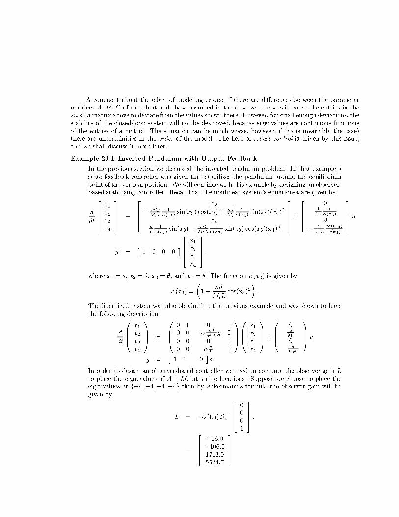
Example 29.1 Inverted Pendulum with Output Feedback

In the previous section we discussed the inverted pendulum problem. In that example a

state feedback controller was given that stabilizes the pendulum around the equilibrium

point of the vertical position. We will continue with this example by designing an observer-based stabilizing controller. Recall that the nonlinear system's equationsa are given by 23232

x1

x2

0

1 1mlg 1 sin(x3) cos(x3) +

ml 1 sin(x3)(x4

)2

�(x3

) Mt

�(x3

)

664

�

g 1 ml 1 1

cos(x3

)x4 L �(x3

)

sin(x3) ; Mt

L �(x3

)

sin(x3) cos(x3)(x4

)2 ; Mt

L �(x3

)2 3

x1

664775

775

664

775

d

dt

;x2

Mt

�(x3

)Mt

L + u0x3

x4

664

x2

x3

775

�

��

� 1 0 0 0y

x4

_where x1

� s, x2

� s_, x3

� �, and x4

� �. The function �(x3) is given by ��

ml

�(x3

) � 1 ; cos(x3)2 :

MtL

The linearized system was also obtained in the previous example and was shown to have

the following description 010 10 101

x1

0 1 0 0 x1

0

�;�

ml

Mt

L

�

BB@�

y � 1 0 0 x:

In order to design an observer-based controller we need to compute the observer gain L

to place the eignevalues of A + LC at stable locations. Suppose we choose to place the

eigenvalues at f;4� ;4� ;4� ;4g then by Ackermann's formula the observer gain will be

given by 2 3

0

BB@

CCA

BB@

CCA

CCA

BB@

CCA

d 00 0 gx2

x2 Mt� + u

00 0 0 1dt

x3

x3

�0 0 �

g 0L

;x4

x4 LMt

L � ;�d(A)O4

;1

664

0

0

775

�

1 2 3 ;16:0

;106:0

�

664

775 1743:0

5524:7

3

x_1 and \hat x_1 x_2 and \hat x_2 2 3

1.5 2

1

ds/d

t 1

s 0.5 0

0

−1−0.5

−1 −2 0 5 10 0 5 10

time time

x_3 and \hat x_3 x_4 and \hat x_4

thet

a

0.4 1

0.5 d

thet

a/dt

0.2

0 0

−0.5

−0.2 −1

−0.4 −1.5 0 5 10 0 5 10

time time

Figure 29.3: Plot of the state variables and the observer variables of the closed-Loop linearized

_system with r � 0 and the initial condition s � 0, s_ � 0, � � :2, � � 0, x1

� 0, x2

� 0, and

x3

� 0, x4

� 0. The solid lines represent the state variables and the dashed lines represent

the observer variables

where in the above expression we have �d(�) � (� + 4)4 . The closed loop system is

simulated as shown in Figure 29.3. Note that the feedback matrix F is the same as was

obtained in the �rst example in this chapter. It is clear that the estimates ^ x1, x 2, ^ x3

and

x 4

converge to the state variables x1, x2, x3

and x4. The initial angle of the pendulum is

chosen to be :2 radians and the initial condition for the observer variables as well as the

other state variables are chosen to be zero, and .

The observer-based controller is applied to the nonlinear model and the simulation is given

in Figure 29.4.

x_1 and \hat x_1 x_2 and \hat x_2 2 3

1.5 2

1 1

ds/d

t

s 0.5 0

0 −1

−0.5 −2

−1 −3 0 5 10 0 5 10

time time

x_3 and \hat x_3 x_4 and \hat x_4

thet

a

d th

eta/

dt

0.4 1.5

10.2

0.5 0

0 −0.2

−0.5

−0.4 −1

−0.6 −1.5 0 5 10 0 5 10

time time

Figure 29.4: Plot of the state variables and the observer variables of the closed-Loop nonlinear

_system with r � 0 and the initial condition s � 0, s_ � 0, � � :2, � � 0, x1

� 0, x2

� 0, and

x3

� 0, x4

� 0. The solid lines represent the state variables and the dashed lines represent

the observer variables

Exercises

Exercise 29.1 Consider the mass-spring system shown in the �gure below.

-x1(t)

-x2(t)

w(t)

-u(t)

- m1

.......................

J �J

J� J....................... m2

k

Let x1(t) denote the position of mass m1, x2(t) the position of mass m2, x3(t) the velocity of mass

m1, x4(t) the velocity of mass m2, u(t) the applied force acting on mass m1, and w(t) a disturbance

force acting on mass m2, k is the spring constant. There is no damping in the system.

The equations of motion are as follows:

x_1(t) � x3(t)

x_2(t) � x4(t)

x_3(t) �

x_4(t) �

;(k�m1)x1(t) + (k�m1)x2(t) + (1�m1)u(t)

(k�m2)x1(t) ; (k�m2)x2(t) + (1�m2)w(t)

The output is simply the position of mass m2, so

y(t) � x2(t)

Assume the following values for the parameters:

m1

� m2

� 1� k � 1

(a) Determine the natural frequencies of the system, the zeros of the transfer function from u to y,

and the zeros of the transfer function from w to y.

(b) Design an observed-based compensator that uses a feedback control of the form u(t) � F x(t)+r(t),

where x(t) is the state-estimate provided by an observer. Choose F such that the poles of the

transfer function from r to y are all at ;1. Design your observer such that the natural frequencies

governing observer error decay are all at ;5.

(c) Determine the closed-loop transfer function from the disturbance w to the output y and obtain

its Bode magnitude plot. Comment on the disturbance rejection properties of your design.

(d) Plot the transient response of the two position variables and of the control when x2(0) � 1 and

all the other state variables, including the compensator state variables, are initially zero.

(e) Plot the transient response of the two position variables and of the control when the system is

initially at rest and the disturbance w(t) is a unit step at time t � 0.

Exercise 29.2 Reduced Order Observer

The model-based observer that we discussed in class always has dimension equal to the dimension of

the plant. Since the output measures part of the states (or linear combinations), it seems natural that

only a subset of the states need to be estimated through the observer. This problem shows how one

can derive a reduced order observer.

Consider the following dynamic system with states x1

2 Rr� x2

2 Rp: � � � �� � � �

x_1

A11

A12

x1

B1� + u�

x_2

A21

A22

x2

B2

and

y � x2:

Since x2

is completely available, the reduced order observer should provide estimates only for x1, and

its dimension is equal to r, the dimension of x1. Thus � �

x 1 x � :

x2

One may start with the following potential observer:

_x 1

� A11x 1

+ A12y + B1u + L(y ; y)

Since y � Cx � x2

(since x2

is known exactly), the correction term in the above equation is equal to

zero (L(y ; y) � 0). This indicates that this proceedure may not work.

Suppose instead, that we de�ne a new variable z � x1

; Lx2, where L is an r � p matrix that we will

choose later. Then if we can derive an estimate for z, denoted by z, we immediately have an estimate

for x1, namely, x1

� z + Lx2.

(a) Express z_ in terms of z� y� and u. Show that the state matrix (matrix multiplying z) is given by

A11

; LA21.

(b) To be able to place the poles of A11

; LA21

in the left half plane, the pair (A11� A21) should be

observable (i.e., a system with dynamic matrix A11

and output matrix A21

should be observable).

Show that this is the case if and only if the original system is observable.

(c) Suggest an observer for z. Verify that your choice is good.

(d) Suppose a constant state feedback matrix F has been found such that A + BF is stable. Since

not all the states are availabe, the control law can be implemented as:

u � F x � F1x 1

+ F2x2

where F � ( F1

F2

) is decomposed conformally with x1

and x2. Where do the closed loop

poles lie� Justify your answer.

Exercise 29.3 (Observers and Observer-Based Compensators) The optimal control in Prob-lem 28.3 cannot be implemented when x is not available to us. We now examine, in the context of the

(magnetic suspension) example in that problem, the design of an observer to produce an estimate x,

and the design of an observer-based compensator that uses this estimate instead of x. Assume for this

problem that the output measurement available to the observer is the same variable y that is penalized

in the quadratic criterion. [In general, the penalized \output" in the quadratic criterion need not be

the same as the measured output used for the observer.]

(a) Design a full-order observer for the original open-loop system, to obtain an estimate x(t) of x(t),

knowing only u and y. The eigenvalues that govern error decay are both to be placed at ;6.

(b) Suppose we now use the control u(t) � F

�x(t)+v(t), where F

� is the same as in (d), (e) of Problem

2, and v(t) is some new external control. Show that the transfer matrix of the compensator,

whose input vector is ( u y )0

and whose output is the scalar f � F

�x, is given by

1 ;

(s + 6)2

[ 6(s + 15) 486(s + 3) ]

Also determine the transfer function from v to y.

(c) As an alternative to the compensator based on the full-order observer, design a reduced-order

observer | see Problem 1(c) | and place the eigenvalue that governs error decay at ;6. Show

that the transfer matrix in (b) is now replaced by

1 ; [6 54(s + 3)]

(s + 6)

and determine the transfer function from v to y.

Exercise 29.4 Motivated by what we have done with observer-based compensators designed via state-space methods, we now look for a direct transform-domain approach. Our starting point will be a given

open-loop transfer function for the plant, p(s)�a(s), with a(s) being a polynomial of degree n that has

no factors in common with p(s). Let us look for a compensator with the structure of the one in Problem

03(b), with input vector ( u y ) , output f that constitutes the feedback signal, and transfer matrix

1 ; [ q(s) r(s) ]

w(s)

where w(s) is a monic polynomial (i.e. the coe�cient of the highest power of s equals 1) of degree n,

while q(s) and r(s) have degrees n ; 1 or less. With this compensator, the input to the plant is given

by u � f + v, where v is some new external control signal.

(a) Find an n-th order realization of the above compensator. (Hint: Use the familiar SISO observer

canonical form, modi�ed for 2 inputs.) (You will not need to use this realization for any of the

remaining parts of this problem | the intent of this part is just to convince you that an n-th

order realization of the compensator exists.)

(b) Show that the transfer function from v to y is

p(s)w(s)

g(s) �

[w(s) + q(s)]a(s) + r(s)p(s)

and argue that the characteristic polynomial of the system must be

[w(s) + q(s)]a(s) + r(s)p(s)

It turns out that, since a(s) and p(s) are coprime, we can choose [w(s) + q(s)] and r(s) to

make the characteristic polynomial equal to any monic polynomial of degree 2n. The following

strategy for picking this polynomial mimics what is done in the design of an observer-based

compensator using state-space methods: pick w(s) to have roots at desirable locations in the

left-half-plane (these will correspond to observer error decay modes)� then pick q(s) and r(s) so

that the characteristic polynomial above equals �(s)w(s), where �(s) is a polynomial of degree

n that also has roots at desirable positions in the left-half- plane. With these choices, we see

that

g(s) � [p(s)w(s)]�[�(s)w(s)] � p(s)��(s)

This compensator has thus shifted the poles of the closed-loop system from the roots of a(s) to

those of �(s), and the roots of w(s) correspond to hidden modes.

(c) Design a compensator via the above route for a plant of transfer function 1�(s2 ; 9), to obtain an

overall transfer function of 1�(s + 3)2 , with two hidden modes at ;6. Compare with the result

in Problem 3(b).

(d) The above development corresponds to designing a compensator based on a full-order observer.

A compensator based on a reduced-order observer | see Problem 1(c) | is easily obtained as

well, by simply making w(s) a monic polynomial of degree n ; 1 rather than n and making any

other changes that follow from this. After noting what the requisite changes would be, design a

compensator for a plant of transfer function 1�(s2 ; 9), to obtain an overall transfer function of

1�(s + 3)2 , with one hidden mode at ;6. Compare with the result in Problem 3(c).

Exercise 29.5 Consider a plant described by the transfer function matrix � 1 1

�

s;1 s;1P (s) � 2s;1 1

s(s;1)

(a) Design a model-based (i.e. observer-based) controller such that the closed loop system has all

eigenvalues at s � ;1.

(b) Suppose that P11(s) is perturbed to

1+�

s;1

. For the controller you designed, give the range of � for

which the system remains stable. Discuss your answer.

s;1

Exercise 29.6 Assume we are given the controllable and observable system x_ (t) � Ax(t) + Bu(t),

z(t) � Cx(t), with transfer matrix P (s). The available measurement is y(t) � z(t) + d(t), where d(t)

is a disturbance signal. An observer for the system comprises a duplicate of the plant model, driven

by the same input u(t), but also by a correction term e(t) � y(t) ; Cx(t) acting through an observer

gain L, which is chosen to obtain stable error dynamics.

For an observer-based stabilizing compensator, suppose we pick u(t) � F x(t)+ r(t)+ v(t), where

x(t) is the estimate produced by an observer, F is the gain we would have used to stabilize the system

under perfect state feedback, r(t) is some external input, and v(t) is the output of a stable �nite

dimensional LTI system whose input is e(t) and whose (proper, rational) transfer function matrix is

Q(s). (The case of Q(s) � 0 constitutes the \core" observer-based stabilizing compensator that we

have discussed in detail in class.) A block diagram for the resulting system is given below.

(a) Show that this system is stable for any stable �nite-dimensional system Q. [Hint: The transfer

function from v to e is equal to zero regardless of what r and d are!]

(b) Obtain a state-space description of the overall system, and show that its eigenvalues are the union

of the eigenvalues of A + BF , the eigenvalues of A + LC, and the poles of Q(s).)

(c) What is the transfer function matrix K(s) of the overall feedback compensator connecting y to

u� Express it in the form K(s) � [W (s) ; Q(s)M(s)];1[J(s) ; Q(s)N(s)], where the matrices

W� M� J� N are also stable, proper rationals.

It turns out that, as we let Q(s) vary over all proper, stable, rational matrices, the matrix K(s)

ranges precisely over the set of proper rational transfer matrices of feedback compensators that stabilize

the closed-loop system. This is therefore referred to as the \Q-parametrization" of stabilizing feedback

compensators.

d

+

�+

�� �� r - u - - y-��

P (s)+��

6+

� ���+ � ���

F Observer

6

+

�+ ;��v y -��

�Q(s)

e

MIT OpenCourseWarehttp://ocw.mit.edu

6.241J / 16.338J Dynamic Systems and Control Spring 2011

For information about citing these materials or our Terms of Use, visit: http://ocw.mit.edu/terms.