68 journal c. chapter 6

68 SOME GENERAL CONSIDERATIONS IN CONTROLLING BIAS

McKinlay, S. (197% The Design and Analysis of the Observational Study-A Review, Journal ofthe American Statistical Association, 70, 503-520.

Mather, H. G., Pearson, N. G., Read, K. L. Q., Shaw, D B., Steed, G. R., Thorne, M. G., Jones, S., Guerrier, C. J., Eraut. C. D., McHugh, P. M., Chowdhurg, N. R., Jafary, M. H., and

, Wallace, T. J. (1971), Acute Myocardial Infarction: Home and Hospital Treatment. British Medical Journal, 3,334-338.

Mosteller, F., and Tukey, J. W. (1977), Data Analysis and Regression, Reading. MA: Addison- Wesley.

Thorndike, F. L. (1972), Regression Fallacies in the Matched Group Experiment, Psychometrika, 7(2), 85-102.

Weisberg, H. I. (1979), Statistical Adjustments and Uncontrolled Studies, Psychological Bulletin, 86,1149-1 164.

C H A P T E R 6

6.1 Effect of Noncomparability 7 1

6.2 Factors Influencing Bias Reduction 74

6.3 Assumptions 77

6.4 Caliper Matching 7 8

6.4.1 Methodology 79

6.4.2 Appropriate Conditions 80

6.4.3 Evaluation of Bias Reduction 8 3

6.5 Nearest Available Matching 84


6.5.2 Appropriate Conditions 8 5

6.5.3 Evaluation of Bias Reduction 8 5

6.6 Stratified Matching 87

6.7 Frequency Matching 88



6.7.3 Evaluation of Bias Reduction 90

6.8 Mean Matching 9 1

6.8.1 Methodology 9 91

6.8.2 Appropriate Conditions 9 1

6.8.3 Evaluation of Bias Reduction 93

6.9 Estimation and Tests of Significance 93

6.10 Multivariate Matching 1 94

6.10.1 Multivariate Caliper Matching 95

6.10.2 Multivariate Stratified Matching 97

6.10.3 Minimum Distance Matching 99

6.10.4 Discriminant Matching 102

6.10.5 Multivariate Matching with Linear Adjustment 102

6.1 1 Multiple Comparison Subjects 103

6.12 Other Considerations 105

6.12.1 Omitted Confounding Variables 105 6.12.2 Errors of Measurement in Confounding Variables 106 6.12.3 Quality of Pair Matches 106

69

6.13 Conclusions Appendix 6A Some Mathematical Details

6A. 1 Matching Model 6A.2 Parallel Linear Regression 6A.3 Parallel Nonlinear Regression

References

MATCHING

108 109 109 109 110 111

The major concern in making causal inferences from comparative studies is that a proper standard of comparison be used. A proper standard of comparison (see Chapter 1) requires that the performance of the comparison group be an adequate proxy for the performance of the treatment group if they had not re- ceived the treatment. One approach to obtaining such a standard is to choose study groups that are comparable with respect to all important factors except for the specific treatment (i.e., the only difference between the two groups is the treatment). Matching attempts to achieve comparability on the important potential confounding factor(s) a t the design stage of the study. This is done by appropriately selecting the study subjects to form groups which are as alike as is possible with respect to the potential confounding variable(s). Thus the goal of the matching approach is to have no relationship between the risk and the potential confounding variables in the study sample. Therefore, these potential confounding variables will not satisfy part 1 of the definition of a confounding variable given at the beginning of Chapter 2, and thereby will not be confounding variables in the final study sample. This strategy of matching is in contrast to the strategy of adjustment, which attempts to correct for differences in the two groups a t the analysis stage.

We stated that matching "attempts to achieve comparability" because it is seldom possible to achieve exact comparability between the two study groups. This is especially true in the case of several confounding variables. To judge how

1 effective the various matching procedures can be in achieving comparability and thus reducing bias in the estimate of the treatment effect, it is necessary to model the relationship between the outcome or response variable and the confounding variable(s) in the two treatment groups. Since much of the research has been done assuming a numerical outcome variable that is linearly related to the confounding variable, we will tend to emphasize this type of relationship. The reader should not believe, however, that matching is applicable only in this case. There are matching techniques which are relatively effective in achieving comparability and reducing bias in the case of nonlinear relationships.

Before presenting the various matching techniques, we shall illustrate in Section 6.1 how making the two treatment groups comparable on an important confounding variable will eliminate the bias due to that variable in the estimate

6.1 EFFECT OF NONCOMPARABILITY 71

of the treatment effect. Section 6.1 expands on material presented in Section 3.2.

The degree to which the two groups can be made comparable depends on (a) how different the distributions of the confounding variable are in the treatment and comparison groups, and (b) the size of the comparison population from which one samples. These factors influence the amount of bias reduction possible using any of the matching techniques, and are discussed in Section 6.2.

In the last introductory section of this chapter, Section 6.3, we list and discuss the conditions under which the results for the various matching techniques are applicable. Although these conditions are somewhat overly restrictive, they are necessary for a clear understanding of the concepts behind the various techniques.

Finally, the main emphasis of this chapter is on the reduction of the bias due to confounding. The other two sources of bias, bias due to model misspecification - and estimation bias, however, can also be present. See Sections 5.4 and 5.5 for a discussion of these other sources of bias. All of the theoretical results that we present are for the case of no model misspecification. This should be kept in mind when applying the results to any study.

6.1 EFFECT OF NONCOMPARABILITY

For the sake of illustration, reconsider the example introduced in Chapter 3, the study of the association between cigarette smoking and high blood pressure. Recall that cigarette smoking is the risk variable and age is an important confounding variable. This last assumption implies that the age distributions of the smokers and nonsmokers must differ: otherwise, age would not be related to the risk variable (i.e., the groups would be comparable with respect to age). We shall further assume that the smokers are generally older (see Figure 3.3) and that the average blood pressure increases with age at the same%ate for both smokers and nonsmokers (see Figure 3.4). Let X denote, age in years and Y denote diastolic blood pressure in millimeters of mercury (mm Hg). The effect of the risk factor, cigarette smoking, can be measured by the difference in average blood pressure for any specific age, and because of the second assumption, this effect will be the same for all ages.

These two assumptions can be visualized in Figure 6.1. Suppose that we were to draw large random samples of smokers and nonsmokers from the populations shown in Figure 3.3. The sample frequency distributions would then be as il- lustrated in Figure 6.1 by the histograms. The smokers in the sample tend to be older than the nonsmokers. In particular, the mean age of the smokers is larger than that of the nonsmokers, Xs > (Notice that the Y axis in Figure 6.1 does not correspond to the ordinate of the frequency distributions.)

MATCHING

Blood pressure

E L ' - . /

I Fs - y ~ s 1 1 True " "" 1 I I -Nonsmokers

I I effect

Figure 6.1 Estimate of the treatment effect for the blood pressure-smoking example.

The second assumption, specifying that the relationship between age and diastolic blood pressure in both groups is linear, is represented by the lines labeled "Smokers" and "Nonsmokers" (as in Figure 3.4). Algebraically, these relationships are:

Ys = as + PX for smokers

YNS = ~ N S + PX for nonsmokers, (6.1)

i where Ys and YNS represent the average blood pressure levels among persons of age X , and ,L? is the rate at which Y, blood pressure, changes for each I-year change in X. [Note that for simplicity of presentation, random fluctuations or errors (Section 2.2) will be ignored for now.] For a specified age, Xo, therefore, the effect of the risk factor is

= (Yfj - (YNS (6.2)

(see Figure 6.1 ). Let us first consider the simplest situation, where there is only one subject

in each group and where each subject is age Xo. We will then have two groups that are exactly comparable with respect to age. The estimate of the treatment

; 6.1 EFFECT OF NONCOMPARABILITY

effect is the difference between the blood pressures of the two subjects. Since the blood pressures of these two subjects are as given in (6.1) with X = Xo, the estimated treatment effect will be as given in (6.2). Thus exact comparability has led to an unbiased estimate of the treatment effect. (Note that the same result would also hold for any nonlinear relationship between X and Y.)

Next consider the estimate of the treatment effect based on all subjects in the two samples. The estimate is found by averaging over all the values of Y in both groups and calculating the difference between these averages:

Thus because of the noncomparability of the two groups with respect to age, the estimate of the risk effect is distorted or biased by the amount P(Xs - XNS). Since we do not know ,B, we cannot adjust for this bias. (An adjustment procedure based on estimating /3 is analysis of covariance; see Chapter 8.) Notice, however, that if we could equalize the two sample age distributions, or in the case considered here of a linear relationship, restrict the sampling so that the two sample means were equal, we would then obtain an unbiased estimate of the treatment effect. By making the groups comparable, one would be assured of averaging over the same values of X .

There are two basic approaches to forming matches to reduce bias due to confounding. These are referred to as pair and nonpair matching. Pair matching methods find a specific match (comparison.subject) for each treatment subject. It is clear that if we restrict the choice of subjects in the two groups such that for every treatment subject with age Xo there is a comparison subject with exactly the same age, then by (6.2) the difference in blood pressures between each matched pair is an unbiased estimate of the treatment effect. Hence the average difference will also be unbiased.

Because of difficulties in finding comparison subjects with exactly the same value of a confounding variable as a treatment subject, various pair matching methods have been developed. For example, if the confounding varjable is numerical, it is practically impossible to obtain exact7,matches for all treatment subjects. An alternative method, caliper matching, matches two subjects if their values of X differ by only a small tolerance (Section 6.4). In the case of a categorical confounding variable, one can use a pair matching method called stratified matching (Section 6.6). However, these methods cannot always guarantee the desired sample size, so another pair matching method, called nearest available pair matching (Section 6.5), was developed by Rubin (1973a).

In the second approach to matching, nonpair matching, no attempt is made to find a specific comparison subject for each treatment subject. Thus there are no identifiable pairs of subjects. There are two nonpair matching methods: frequency and mean matching. In frequency matching, Section 6.7, the distri-

74 MATCHING

bution of the confounding variable in the treatment group is stratified and one attempts to equalize the two distributions by equalizing the number of treatment and comparison subjects in each stratum. Mean matching, Section 6.8, attempts to reduce the amount of bias by equating just the sample means rather than attempting to equalize the two distributions as in the previous methods. The comparison group, which is of the same size as the treatment group, thus consists of those subjects whose group mean is closest to the mean of the treatment group.

6.2 FACTORS INFLUENCING BIAS REDUCTION

None of the matching methods requires the fitting of a specific model for the relationship between the response and the confounding variables. The effectiveness of a matching procedure, however, will depend on the form of the relationship between the response and the confounding variables. In addition, the effectiveness depends on the following three factors: (a) the difference between the means of the treatment and comparison distributions of a confounding variable, (b ) the ratio of the population variances, and (c) the size of the control sample from which the investigator forms a comparison group. These three factors will now be discussed in detail.

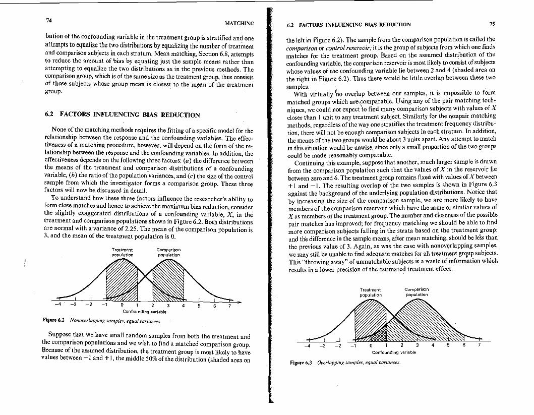
To understand how these three factors influence the researcher's ability to form close matches and hence to achieve the maximum bias reduction, consider the slightly exaggerated distributions of a confounding variable, X, in the treatment and comparison populations shown in Figure 6.2. Both distributions are normal with a variance of 2.25. The mean of the comparison population is 3, and the mean of the treatment population is 0.

Treatment Comparison ~ o ~ u l a t i o n ~ o ~ u l a t i o n

Confounding variable

Figure 6.2 Nonoverlapping samples, equal variances.

Suppose that we have small random samples from both the treatment and the comparison populations and we wish to find a matched comparison group. Because of the assumed distribution, the treatment group is most likely to have values between -1 and + 1, the middle 50% of the distribution (shaded area on

6.2 FACTORS INFLUENCING BIAS REDUCTION 75

the left in Figure 6.2). The sample from the comparison population is called the comparison or control reseruoir; it is the group of subjects from which one finds matches for the treatment group. Based on the assumed distribution of the confounding variable, the comparison reservoir is most likely to consist of subjects whose values of the confounding variable lie between 2 and 4 (shaded area on the right in Figure 6.2). Thus there would be little overlap between these two samples. 1

With virtually no overlap between our samples, it is impossible to form matched groups which are,comparable. Using any of the pair matching techniques, we could not expect to find many comparison subjects with values of X closer than 1 unit to any treatment subject. Similarly for the nonpair matching methods, regardless of the way one stratifies the treatment frequency distribution, there will not be enough comparison subjects in each stratum. In addition, the means of the two groups would be about 3 units apart. Any attempt to match in this situation would be unwise, since only a small proportion of the two groups could be made reasonably comparable.

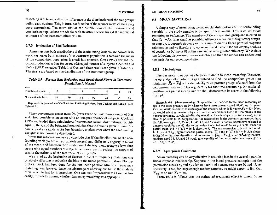
Continuing this example, suppose that another, much larger sample is drawn from the comparison population such that the values of X in the reservoir lie between zero and 6. The treatment group remains fixed with values of X between + 1 and - 1. The resulting overlap of the two samples is shown in Figure 6.3 against the background of the underlying population distributions. Notice that by increasing the size of the comparison sample, we are more likely to have members of the comparison reservoir which have the same or similar values of X as members of the treatment group. The number and closeness of the possible pair matches has improved; for frequency matching we should be able to find more comparison subjects falling in the strata based on the treatment group; and th'e difference in the sample means, after mean matching, should be le'ss than the previous value of 3. Again, as was the case with nonoverlapping samples, we may still be unable to find adequate matches for all treatment grgup subjects. This "throwing away" of unmatchable subjects is a waste of information which results in a lower precision of the estimated treatment effect.

Treatment Comparison population population


Figure 6.3 Overlapping samples, equal variances

76 MATCHING

Now consider what would happen if the population variances of the confounding variable were not equal. In particular, suppose that the variance of the treatment population, a:, remains at 2.25, while the variance of the comparison population, a;, is 9.0. (Again, this is a slightly exaggerated example but is useful to illustrate our point.) With the treatment sample fixed, random sampling from the comparison population would most likely result in a sample as shown by the shading in Figure 6.4. Notice the amount of overlap that now exists between the treatment group and the comparison reservoir. There are clearly more subjects in the comparison reservoir, with values of the confounding variable between + 1 or - 1, than in the previous example (Figure 6.3).

Treatment population


Figure 6.4 Overlapping samples. unequal variances.

After comparing these examples, the relationship among the three factors-the difference between the population means of the two distributions, the ratio of the population variances, and the size of the comparison reservoir- should be clear. The farther apart the two population means are, the larger the comparison reservoir must be to find close matches, unless the variances are such that the two population distributions overlap substantially.

To determine numerically the bias reduction possible for a particular matching technique, it is necessary to quantify these three factors. Cochran and Rubin (1973) chose to measure the difference between the population means by a quantity referred to as the initial difference. This measure, Bx, may be viewed as a standardized distance measure between two distributions and is defined as

The eta terms, vl and TO, denote the means of the treatment and the comparison populations, respectively. Similarly, u: and u; represent the respective population variances.

6.3 ASSUMPTIONS 77

the variance of the comparison population increased to 9, however, the initial difference was equal to 1.3 and the two distributions overlapped more.

The ratio of the treatment variance to the comparison variance, u:/ui, is the second important factor in determining the number of close matches that can be formed, and hence the bias reduction possible. Generally, the smaller the ratio, the easier it will be to find close matches.

The last factor is the size of the comparison reservoir from which one finds matches. In the previous examples we assumed that the random sample from the treatment population was fixed. That is, we wanted to find a match for every subject in that sample and the subjects in the treatment group could not be changed in order to find matches. Removal of a treatment subject was the only allowable change if a suitable match could not be found. This idea of a fixed treatment group is used in the theoretical work we cite and is perhaps also the most realistic approach in determining the bias reduction possible. An alternative and less restrictive approach assumes that there exists a treatment reservoir from which a smaller group will be drawn to form the treatment group. Such an approach would allow for more flexibility in finding close matches.

In the following methodological sections the size of the comparison reservoir is stated relative to the size of the fixed treatment group. Thus a comparison reservoir of size r means that the comparison reservoir is r times larger than the treatment group. Generally, r is taken to be greater than 1.

6.3 ASSUMPTIONS

In discussing the various matching procedures, we shall make the following assumptions:

1. There is one confounding variable. 2. The risk variable in cohort studies or the outcome variable idcase-control

studies is dichotomous. 3. The treatment effect is constant for all values of the confounding variable.

(This is the no interaction assumption of Section 3.3.) 4. For cohort studies we wish to form treatment and comparison groups of

equal size. (For case-control studies, we would construct case and control groups of equal size.) 1

5. The treatment group (or case group) is fixed.

The assumption of only one confounding variable is made for expository purposes. In Section 6.1 0 we will discuss matching in the case of multiple confounding variables. The second assumption corresponds to the most common situation where matching is used. Matching cannot be used if the risk variable

78 MATCHING

in cohort studies or the outcome variable in case-control studies is numerical. The third assumption of no interaction, or parallelism, is crucial for estimating the treatment effect. Researchers should always be aware that implicitly they are making this assumption and when possible they should attempt to verify it. For example, in Section 5.2, we discuss how the assumption of parallelism may be unjustified when one is dealing with fallible measurements. If this assumption is not satisfied, the researcher will have to reconsider the advisability of doing the study or else to report the study findings over the region for which the assumption holds. The fourth assumption, that the treatment and comparison groups are of equal size, is also made for expository purposes. In addition, the efficiency of matching is increased with equal sample sizes for a given total sample size. In Section 6.1 1 we consider the case of multiple comparison subjects per treatment subject. The last assumption of a fixed treatment group is one of the assumptions under which most of the theoretical work is done. A fixed treatment group is typically the situation in retrospective studies where the group to be studied, either case or exposed, is clearly defined.

While the type of study has no effect on the technique of matching, the forms of the outcome and confounding variables do. The various matching techniques can be used in either case-control or cohort studies. The only difference is that in a cohort study one matches the groups determined by the risk or exposure factor, whereas in a case-control study, the groups aredetermined by the outcome variable. Throughout this chapter, any discussion of a cohort study applies also to a case-control study, with the roles of the risk and outcome variables reversed.

The form of the risk or outcome variable and the confounding variables (i.e., numerical or categorical) determines the appropriate matching procedure and whether matching is even possible. If the confounding variable is of the unordered categorical form, such as religion, there is little difficulty in forming exact matches. We shall, therefore, make only passing reference to this type of con-

1 founding variable. Instead, we shall emphasize numerical and ordered categorical ' confounding variables, where the latter may be viewed as having an underlying numerical distribution. Numerical confounding variables are of particular im- portance because exact matching is very difficult in this situation. Most of the theoretical work concerning matching has been done for a numerical confounding variable and dichotomous risk variable (cohort study).

6.4 CALIPER MATCHING

Caliper matching is a pair matching technique that attempts to achieve comparability of the treatment and comparison groups by defining two subjects to be a match if they differ on the value of the numerical confounding variable,

6.4 CALIPER MATCHING 79

X, by no more thah a small tolerance, E . That is, a matched pair must have the property that

1x1 - Xol 5 E .

The subscript 1 denotes treatment group and 0 denotes comparison group. By selecting a small-enough tolerance t, the bias can in principle be reduced to any desired level. However, the smaller the tolerance, the fewer matches will be possible, and in general, the larger must be the reservoir of potential comparison subjects.

Exact matching corresponds to caliper matching with a tolerance of zero. In general, though, exact matching is only possible with unordered categorical confounding variables. Sometimes, however, the number of strata in a categorical variable is so large that they must be combined into a smaller number of strata. In such cases or in the case of ordered categorical variables, the appropriate pair matching technique is stratified matching (Section 6.6).

6.4.1 Methodology

To illustrate caliper matching we shall consider the cohort study of the association of blood pressure and cigarette smoking.

Example 6.1 Blood pressure and cigarette smoking: Suppose that a tolerance of 2 years is specified and that the ages in the smokers group are 37,38,40,45, and 50 years. (We shall assume that the smoker and nonsmoker groups are comparable on all other important variables.) A comparison reservoir twice the size ( r = 2) of the smoking group consists of nonsmokers of ages 25, 27, 32, 36,38,40,42,43,49, and 53 years. The estimated means of the two'groups are 42.0 and 38.5 years, respectively. The ratio of the estimated variances, s$/sLs, is 0.37 = 29.50/79.78.

The first step in forming the matches is to list the smokers and determine the corresponding comparison subjects who are within the 2-year tolerance from each smoker. For our example, this results in the possible pairing given in Table 6. la. *

Table 6.1a Potential Caliper Matches for Example 6.1

Smokers Nonsrnokers

It is clearly desirable to form matches for all the treatment subjects that are as close as possible. Thus the matched pairs shown in Table 6.lb would be formed.

MATCHING

Table 6. l b Caliper-Matched Pairs

Smokers Nonsmokers

Notice that if the 49-year-old nonsmoking subject had not been in the reservoir, we would not have been able to match all five smokers. We might then have decided to keep the first four matches and drop the 50-year-old smoker from the study. This results in a loss of precision, because the effective sample size is reduced. Alternatively, the tolerance could beincreased to 3 years and the 50-year-old smoker matched with the 53-year-old nonsmoker. The latter approach does not result in lower precision, but the amount of bias may increase. Finally, had there been two or more comparison subjects with the same value of X, the match subject should be chosen randomly.

In Example 6.1 we knew the composition of the comparison reservoir before the start of the study. Often, however, this is not the case. Consider, for example, a study of the effect of specially trained nurses aids on patient recovery in a hospital. Such a study would require that the patients be matched on impottant confounding variables as they entered the hospital. When the comparison reservoir is unknown, the choice of a tolerance value that will result in a sufficient number of matched pairs can be difficult. The researcher cannot scan the reservoir, as we did in the example, and discover that the choice of E is too small. For this reason, using caliper matching in a study where the comparison reservoir is unknown can result in matched sample sizes that are too small. In such a situation, the researcher can sometimes attempt to get a picture of the potential comparison population through records (i.e., historical data).

I

6.4.2 Appropriate Conditions

Caliper matching is appropriate regardless of the form of the relationship between the confounding and outcome variables (or risk variable in case-control studies). In this section we demonstrate how caliper matching is effective in reducing bias in both the linear and nonlinear cases.

Linear Case. To understand how caliper matching works in the linear case, let us consider the estimate of the treatment effect or risk effect of smoking on blood pressure based on a 45-year-old smoker and a 43-year-old nonsmoker in Example 6.1. Assume that blood pressure is linearly related to age and that the relationships are the same for both groups, with the exception of the intercept values. Figure 6.5 represents this situation.

F j 6.4 CALIPER MATCHING 81 i

! .f Blood pressure1

effect,

Figure 6.5 Esrirnafe of rrearmenr effecr-linear relarionship.

The estimate of the risk effect is shown by the large brace to the left in Figure 6.5. The amount of bias or distortion is shown by the small brace labeled "Bias." Relating this example to (6.3), we see that the bias is equal to the unknown regression coefficient p, multiplied by the difference in the values of the confounding variable. In the case of these two subjects, the bias is 2p. This is the maximum bias allowable under the specified tolerance for each individual estimate of the treatment effect, and consequently for the estimated treatment effect, based on the entire matched comparison group. 7

When we average the ages in Table 6.16, we find that the mean age of the smokers is 42.0 years; of the nonsmokers comparison group, 41.2 years; and for the comparison reservoir, 38.5 years. Caliper matching thus reduced the difference in means from 3.5 (= 42.0 - 38.5) to 0.8 (= 42.0 - 41.2). In general, the extent to which the bias after matching, 0.8P in this case, is less than the maximum possible bias, 2P in this case, will depend on the quantities discussed in Section 6.2: the difference between the means of the two populations, the ratio of the variances and the size of the comparison reservoir as well as the tolerance.

Nonlinear Case. Let us now consider the case where the response and the confounding variable are related in a nonlinear fashion. To illustrate the effect of caliper matching in this situation, we shall assume that blood pressure is related to age squared. Algebraically this relationship between the response Y and

82

age, X, can be written as

MATCHING

where a is the intercept. The estimate of the treatment effect assuming that Y is numerical is

- yS - YNs = as - aNs + P (3 -?&,I. (6.5)

Hence any bias is a function of thedifference in the means of age squared. Note that the means of the squared ages are different from the squares of the mean ages. Again let us visualize this relationship in Figure 6.6.

~ t o o d pressure !

Estimated effect,

'S - 'NS

True effect

13 ias

I I I > 43 45 Age

I Figure 6.6 Estimate of treatment effect-nonlinear relationship.

The individual estimate of the treatment effect determined from the matched pair of a 45-year-old smoker and a 43-year-old nonsmoker is shown in Figure 6.6 by the large brace to the left. This estimate can be compared to the true treatment effect shown by the topmost smaller brace. The bias is the difference between the two and is indicated by the second small brace. From (6.5) we obtain the bias as

If we were using the matched groups from Example 6.1, upon averaging over the two groups we would find that the estimate of the treatment effect would

6.4 CALIPER MATCHING 83

be biased by the amount

P (z - sNs) = P(69.6).

It is important to realize that equality of the means of the two groups is not enough to ensure an unbiased estimate of the treatment effect if the relationship between the response and the confounding variable is nonlinear. Equality of the means yields unbiased estimates only in the linear case.

6.4.3 Evaluation of Bias Reduction

So far we have only demonstrated how caliper matching can reduce the bias due to confounding. In this section we present theoretical results concerning the bias reduction one can expect using caliper matching in the linear case. The estimator of the treatment effect is the mean difference in response. The effectiveness of caliper matching and all other matching techniques is examined relative to estimating the treatment effect from random samples, where the confounding variable is not taken into account. (For a definition of the measure of effectiveness, the expected percent reduction in bias, see Cochran and Rubin, 1973.)

Table 6.2 gives an indication of the expected percent bias reduction for different tolerance values. The results are independent of the sample size and reservoir size. They were derived assuming that the initial difference between the two populations is less than 0.5 (i.e., Bx < 0.5), thaythe distributions of the confounding variable are normal, and that the outcome is linearly related to the confounding variable. Notice that the tolerance is specified in terms of a proportion, a, of a standard deviation. It appears that tight caliper matchingii.e., a = 0.2) can be expected to remove nearly all the bias in the treatment effect relative to random sampling. It also appears that the ratio of the variances (i.e., crT/a;) has a negligible effect on the percent reduction in bias. ,

Table 6.2 Percent Bias Reduction for Caliper Matching*

a uf / u; = '12 u:/u; = 1 u:/uf = 2

0.2 99 99 98 0.4 96 95 93 0.6 9 1 89 86 0 R 86 82 77

Reprinted, by permission of the Statistical Publishing Society, from Cochran and Rubin (1973), Table 2.3.1.

* Tolerance e = a d ( u : + 4 1 2 .

84 MATCHING

One can use this table to get some indication of bias reduction to be expected for different tolerances if the values or estimates of the population variances are known and if Bx < 0.5. Suppose we knew that a:/ai = l/2, where a: = 4; then if we took a = 0.8, we could expect about 86% of the bias to be removed. The tolerance would be 0.8 4- = 1.96. If we used a = 0.4, we could expect to remove 96% of the bias over random sampling and the tolerance would be 0.98.

As we have mentioned previously, the major disadvantage of caliper matching is the need for the comparison reservoir to be large. In their theoretical work, Cochran and Rubin did not take into account the possibility that the desired number of matches would not be found from the comparison reservoir, although the probability of this occurrence is nonnegligible. Nor are the results known for distributions other than normal. Most likely, the results presented are applicable to symmetric distributions, but the case of skew distributions has not been investigated for caliper matching.

6.5 NEAREST AVAILABLE MATCHING

In some situations when caliper matching is performed with a small tolerance, there is a nonnegligible probability that some individuals cannot be matched. To avoid this problem, Rubin (1973a, b) developed a method known as nearest available pair matching. We shall refer to this matching procedure as nearest available matching. This method ensures that the desired number of matches are obtained by being less restrictive in deciding what a match is. A match is formed by finding the closest possible comparison subject for each individual in the treatment group from the yet-unmatched individuals in the comparison reservoir. Since nearest available matching does not use a fixed tolerance as does caliper matching, the reservoir does not have to be larger than the treatment

I group. However, the matches are not guaranteed to be as close as those found under caliper matching.

6.5.1 Methodology

There are three variants of nearest available matching, each based on a particular ordering of the subjects in the treatment group with respect to the confounding variable. The specification of the ordering completely defines the pair matching method. In one variant of the method, referred to as random-order nearest available matchjng, the N treatment subjects are randomly ordered on the values of the confounding variable, X. Let us denote these ordered values by X11 to X I N . Starting with X l l , a match is defined as that subject from the comparison reservoir whose value Xoj is nearest X 1 1 . The matches are therefore assigned to minimize 1x11 - XoJ 1 for all subjects in the comparison reservoir.

6.5 NEAREST AVAILABLE MATCHING 85 i,

If there are ties (i.e., two or more comparison subjects for whom 1x1 - XoJ 1 ! is a minimum), the match is formed randomly. The nearest available partner 1 for the next treatment subject with value X12 is then found from the remaining

E subjects in the reservoir. The matching procedure continues in this fashion until

t matches have been found for all N treatment subjects. , The other two variants of nearest available matching result from ranking the t-

members of the treatment group on confounding variable values from the highest to the lowest (HL) value or from the lowest to the highest (LH) value. Matches

: are then sought starting with the first ranked treatment subject, as for the random-order version.

Example 6.2 Nearest available matching: Suppose that in a blood pressure study, \

there are three smokers with ages 40,45, and 50, and five nonsmokers in the reservoir with ages 30, 32,46,49, and 55. In addition, suppose that the randomized order of the smokers' ages is 40, 50, and 45. Then the random-order nearest available matching technique will match the 40-year-old smoker with the 46-year-old nonsmoker, the 50- year-old smoker with the 49-year-old nonsmoker, and the 45-year-old smoker with the 55-year-old nonsmoker.

In the case of the other two variants, the following matches would be made: for HL, ' the 50-year-old with the 49-year-old, the 45-year-old with the 46-year-old, and the

40-year-old with the 32-year-old; for LH, the 40-year-old with the 46-year-old, the 45-year-old with the 49-year-old, and the 50-year-old with the 55-year-old. Notice in this example that each variant resulted in different matched pairs.


Nearest available matching is similar to caliper matching except that there is no fixed tolerance. Based on the prior discussion of caliper matching and some theoretical results, it follows that nearest available matching is effective in removing bias due to confounding if the relationship between the response and confounding variables is linear. For nonlinear relationships, no results are

Y available.

The main-difficulty in discussing what conditions are most appropriate for using nearest available matching is the fact that the reduction in bias is so strongly influenced by the closeness of the distributions of the treatment group and the comparison reservoir. If there is a large overlap between the two groups of subjects, nearest available matching will be very similar to caliper matching with a suitably large tolerance. If, however,there is a moderate to small amount of overlap, the desired number of matches will be found, but the final amount of bias in the estimate of the treatment effect may be large.


In selecting a particular nearest available matching procedure, an investigator may want to base his or her choice primarily on the percent reduction in bias

86 MATCHING

obtainable. Assuming a linear relationship between the response and confounding variables, Cochran and Rubin (1973) performed a simulation study to determine which of the three nearest available matching estimators was least biased. They also assumed that the confounding variable was normally distributed with the mean of the treatment population greater than the mean in the comparison population (q l > 90). Their results showed that the percent reduction in bias was largest for the low-high nearest available matching and smallest for the high-low variant.

Because nearest available matching does not guarantee as close matches as are possible with caliper matching, Rubin (1973a) also compared the closeness of the matches obtained by the three procedures as measured by the average of the squared error ( X I - X O ) ~ within pairs. When the procedures were judged by this criterion, the order of performance was reversed. The H L nearest available matching had the lowest average squared error and the L H had the largest. This result is not too surprising, considering the relationship between the population means (ql > qo). The HL procedure would start with the treatment subject who is likely to be the most difficult to match: namely, the one with the largest value of X. This would tend to minimize the squared within-pair difference.

Since the differences between the three matching procedures are small on both criteria, random-order nearest available matching appears to be a rea- sonable compromise. In Table 6.3, from Cochran and Rubin (1973), results of the percent reduction in bias are summarized for random-order nearest available matching as a function of the initial difference, the values of the ratio of the population variances, and sizes of the reservoir. Results for the number of matches N = 25 and N = 100 (not shown) differ only slightly from those for N = 50.

j Table 6.3 Percent Bias Reduction for Random-Order Nearest Available Matching: X Normal: N = 50*

- -

2 99 98 84 92 87 69 66 59 51 3 100 99 97 96 9 5 84 79 75 63 4 100 100 99 98 97 89 86 81 71


* X = confounding variable; Bx = initial difference; r = ratio of the size of the comparison reservoir and the treatment group; = variance of confounding variable in the treatment population; a: = variance of confounding variable in the comparison population.

6.6 STRATIFIED MATCHING 87

With this method, the percent reduction in bias decreases steadily as the initial difference between the normal distributions of the confounding variable increases from to 1 . In contrast with results reported in Table 6.2 for caliper matching, the percent reduction in bias does depend on the ratio of the population variances. Based on Table 6.3, random-order nearest available matching does best when at/ai = v2. When 771 > 770 and a; > a:, large values of the confounding variable in the treatment group, the ones most likely to cause bias, will receive closer partners out of the comparison reservoir than if a; < a:.

Investigators planning to use random-order nearest available matching can use Table 6.3 to obtain an estimate of the expected percent bias reduction. Suppose an estimate of the initial difference Bx is '12, with a:/a; = 1 , and it is known that the reservoir size is 3 times larger than the treatment group (r = 3). It follows that random-order nearest available matching results in an expected 95% reduction in bias.

6.6 STRATIFIED MATCHING

Stratified matching is an appropriate pair matching procedure for categorical confounding variables. If, like sex or religious preference, the variable is truly categorical, with no underlying numerical distribution, the matches are exact and no bias will result. Often, however, the confounding variable is numerical but the investigator may choose to work with the variable in its categorical form. Suppose, for example, that in the study of smoking and blood pressure, all the subjects were employed and that job anxiety is an important confounding variable. The investigator has measured job anxiety by a set of 20 true-false questions so that each subject can have a score from 0 to 20. Such a factor is very difficult to measure, however, and the investigator may decide that it is more realistic and more easily interpretable to simply stratify the rangemf scores into low anxiety, moderate anxiety, and high anxiety. Having formed these three strata, the investigator can now randomly form individual pair matches within each stratum. An example of this procedure in the case of multiple confounding variables is given in Section 6.1 1 .

The only theoretical paper discussing the bias reduction properties of stratified matching is that of McKinlay (1975). She compared stratified matching to various stratification estimators (Section 7.6) for a numerical confounding variable converted to a categorical variable. She considered various numbers of categories and a dichotomous outcome. She found that the estimator of the odds ratio from stratified matched samples had a larger mean squared error and, in some of the cases considered, a larger bias than did the crude estimator, which ignores the confounding variable. (Stratified matching is compared with

88 MATCHING

stratification in Section 13.2.2.) The mean squared error results are due in part to the loss of precision caused by an inability to find matches for all the treatment subjects. This point is considered further in Section 13.2.

6.7 FREQUENCY MATCHING

Frequency matching involves stratifying the distribution of the confounding variable in the treatment group and then finding comparison subjects so that the number of treatment and comparison subjects is the same within each stratum. This is not a pair matching method, and the number of subjects may differ across strata.

For the sake of illustration we shall concentrate on the case of a numerical response. This will allow us to demonstrate more easily how frequency matching helps to reduce the bias. Because frequency matching is equivalent to stratification with equal numbers of comparison and treatment subjects within each stratum, we leave the discussion of the various choices of estimators in the case of a dichotomous response to Chapter 7.

6.7.1 Methodology

Frequency matching is most useful when one does not want to deal with pair matching on a numerical confounding variable or an ordinal measure of an underlying numerical confounding variable. An example of the latter situation is initial health care status, where the categories reflect an underlying continuum of possible statuses. In either case, the underlying dist$bution must be stratified. Samples are then drawn either randomly or by stratified sampling from the comparison reservoir in such a way that there is an equal number of treatment and comparison subjects within each stratum. Criteria for choosing the strata

j are discussed in Section 6.7.3 after we have presented the estimator of the treatment effect.

Example 6.3 Frequency matching: Let us consider the use of frequency matching in the smoking and blood pressure study. Suppose that the age distribution of the smokers was stratified into 10-year intervals as shown on the first line of Table 6.4, and that 100 smokers were distributed across the strata as shown on the second line of the table. The third line of the table represents the results of a random sample of 100 nonsmokers from the comparison reservoir. Notice that since frequency matching requires the sample sizes to be equal within each stratum, the investigator needs to draw more nonsmokers in all strata except for ages 51 to 60 and 71 to 80. In these two strata the additional number of nonsmokers would be dropped from the study on a random basis. (Note that stratified sampling, if possible, would have avoided the problem of too few or too many persons in a stratum.)

6.7 FREQUENCY MATCHING

Table 6.4 Smokers and Nonsmokers Stratified by Age

Age 11-20 21-30 31-40 41-50 51-60 61-70 71-80 Total

Smokers 1 3 10 2 1 30 25 10 100 Nonsmokers 0 2 8 20 32 20 18 100


Frequency matching is relatively effective in reducing bias in the parallel linear response situation provided that enough strata are used. We shall explain this by means of simple formulas for the estimator of the treatment effect assuming a numerical response.

Recall from Section 6.1 that we can represent the linear relationship between the response Y and the confounding variable X by

Y1 = a1 + OXl in the treatment group (6.6)

Yo = QIO + PXo in the comparison group. 1

In general, the estimator of the treatment effect in the kth stratum is

where a bar above the variables indicates the mean calculated for the kth stratum. The bias in the kth stratum is P(xlk - Xok).

Clearly, the maximum amount of distortion in the estimate from the kth stratum occurs when Xlk - XOk is maximized. The maximum value is then P times the width of the kth stratum.

One overall estimate of the treatment effect is the weighted combination of the individual strata differences in the response means:

where nk is the number of treatment or comparison subjects in the kth stratum (k = 1, 2, . . . , K) and N is the total number of treatment subjects. Rewriting (6.8) in terms of treatment effect and regression coefficients, we obtain, using (6.71,

From (6.9) we see that the amount of bias reduction possible using frequency

MATCHING

matching is determined by the difference in the distributions of the two groups within each stratum. This, in turn, is a function of the manner in which the strata were determined. The more similar the distributions of the treatment and comparison populations are within each stratum, the less biased the individual estimates of the treatment effect will be.


Assuming that both distributions of the confounding variable are normal with equal variances but the mean of the treatment population is zero and the mean of the comparison population is small but nonzero, Cox (1957) derived the percent reduction in bias for strata with equal number of subjects. Cochran and Rubin (1973) extended Table 1 of Cox, and these results are given in Table 6.5. The strata are based on the distribution of the treatment group.

Table 6.5 Percent Bias Reduction with Equal-Sized Strata in Treatment Population: X Normal

Number of strata: 2 3 4 5 6 8 10

% reduction in bias: 64 79 86 90 92 94 96


These percentages are a t most 2% lower than the maximum amount of bias reduction possible using strata with an unequal number of subjects. Cochran (1 968) extended these calculations for some nonnormal distributions: the chi- square, the t, and the beta, and he concluded that the results given in Table 6.5 can be used as a guide to the best boundary choices even when the confounding variable is not normally distributed.

! I From this information we can conclude that if the distributions of the con-

founding variable are approximately normal and differ only slightly in terms of the mean, and based on the distribution of the treatment group we form four strata with equal numbers of subjects, we can expect to reduce the amount of bias in the estimate of the treatment effect by 86%.

We stated a t the beginning of Section 6.7.2 that frequency matching was relatively effective in reducing the bias in the linear parallel situation. No theoretical work has been done for the nonlinear parallel situation. Frequency matching does, however, have the advantage of allowing one to use the analysis of variance to test for interactions. One can test for parallelism as well as lin- earity, thus determining whether frequency matching was appropriate.

5

I

6.8 MEAN MATCHING

6.8 MEAN MATCHING

A simple way of attempting to equate the distributions of the confounding variable in the study samples is to equate their means. This is called mean matching or balancing. The members of the comparison group are selected so that 1x1 -Xol is as small as possible. Although mean matching is very simple to employ, it depends strongly on the assumption of a linear parallel response relationship and we therefore do not recommend its use. One can employ analysis of covariance (Chapter 8) in this case and achieve greater efficiency. We include the following discussion of mean matching so that the reader can understand the basis for our recommendation.

6.8.1 Methodology 1

There is more than one way to form matches in mean matching. However, the only algorithm which is guaranteed to find the comparison group that minimizes 1x1 - xol is to calculateXo for all possible groups of size N from the comparison reservoir. This is generally far too time-consuming. An easier algorithm uses partial means, and we shall demonstrate its use with the following example.

Example 6.4 Mean matching: Suppose that we decided to use mean matching on age in the blood pressure study, where we have three smokers, aged 40,42, and 50 years. First, we would calculate the mean age of the smokers, which is 45 years (Xs = 45). Next, we would select successive subjects from the nonsmokers such that the means of the nonsmokers ages, calculated after the selection of each subject (partial means), are as

E close as possible to 45. Suppose that the nonsmokers in the comparison reservoir have the following ages: 32,35,40,41,45,47, and 55 years. The first nonsmoker selected as a match would be age 45; the second subject selected would be 47 years old, since the partial mean, (45 + 47)/2 = 46, is closest to 45. The last nonsmoker to be selected would be 41 years of age, again since the partial mean, (2/d (461+ (It3) (41) = 44.3, is closest to&. Note that this algorithm did not minimize IXs - XNsl, since chgosing the nonsmokers aged 35,45, and 55 would give equality of the two sample mean ages [(35 + 45 + 5913 = 451.


Mean matching can be very effective in reducing bias in the case of a parallel linear response relationship. Suppose in the blood pressure example that the population means gs and ~ N S for smokers and nonsmokers were 50 and 45, respectively. Then, for large enough random samples, we might expect to find that xNS = 45. and Xs = 50.

From (6.3) it follows that the estimated treatment effect is biased by an

MATCHING

amount equal to P ( x s - XNS) = 5P. However, if mean matching had been used to reduce -XNsJ to, say, 0.7, as in Example 6.4, then the bias in (Fs - FNs) would have been reduced by 86% (= 4.315.0). (The initial difference in the means due to random sampling is 5.0.)

Mean matching is not effective in removing bias in the case of a parallel nonlinear response relationship (see Figure 6.7). Assume that in another blood pressure study three smokers of ages 30,35, and 40 years were mean-matched with three nonsmokers of ages 34, 35, and 36 years, respectively. Their blood pressures are denoted by X in Figure 6.7. Notice that unlike the previous linear situ-ations. FS and FNS do not correspond to the mean ages xs and dNs. They will both be greater than the values of Y which correspond to the means due to the nonlinearity. Here (Ys - YNS) is an overestimate of the treatment effect. The estimate should be equal to the length of the vertical line, which represents the treatment effect. In general, the greater the nonlinearity, the greater the overestimation or bias will be, in general.

Blood pressure

1 I Smokers

Estimated effect,

Y, - FNS

Figure 6.7 Mean matching in a nonlinear parallel relationship. X, blood pressure for a specific age;@, blood pressure corresponding to mean age in either group.

6.9 ESTIMATION AND TESTS OF SIGNIFICANCE 93


Cochran and Rubin (1973) have investigated the percentage of bias reduction possible using the partial mean algorithm presented in Section 6.8.1 under the assumptions of a linear parallel relationship, a normally distributed confounding variable, and a sample size of 50 in the treatment group. They found that, except in the cases where the initial difference Bx = 1, mean matching removes es- sentially all the bias. In addition, its effectiveness increases with the size of the comparison reservoir. The bias that results from improper use of mean matching (i.e., in nonlinear cases) has not been quantified.

6.9 ESTIMATION AND TESTS OF SIGNIFICANCE

In this section we indicate the appropriate tests of significance and estimators of the treatment effect for each matching technique. Because the choice of test and estimator depends on the form of the outcome variable, we begin with the numerical case followed by the dichotomous case. Also, in keeping with the general intent of this book, we do not give many details on the test statistics but rather cite references in which further disclission may be found. The tests and estimators for frequency-matched samples are the same as for stratification and are discussed in greater detail in Chapter 7.

In the case of a numerical outcome variable for which one of the pair matching methods (caliper, nearest available, or stratified) has been used, the correct test of significance for the null hypothesis of no treatment effect is the paired-t test (see Snedecor and Cochran, 1967, Chap. 4). This test statistic is the ratio of the mean difference, which is the estimate of the treatment effect, to its standard error. The difference between the paired-t test and the usual t test for independent (nonpaired) samples is in the calculation of the standard error.

If in the case of a numerical outcome variable, frequency matck$ng has been used, the standard t test is appropriate, with the standard error determined by an analysis of variance. (See Snedecor and Cochran, 1967, Chap. 10, for a discussion of the analysis of variance.) The treatment effect is estimated by the mean difference. If, however, the within-stratum variances are not thought to be equal, then, as in the case of stratification, one should weight inversely to the variance (see Section 7.7 and Kalton, 1968). In the case of mean matching, the correct test is again the t test. The standard error, however, must be calculated from an analysis of covariance (see Greenberg, 1953).

When the outcome variable is dichotomous, as discussed in Chapter 3, the treatment effect may be measured by the difference in proportions, the relative risk, or the odds ratio. The estimator of the difference in rates is the difference between the sample proportions, pl - po. This is an unbiased estimator if the

94 MATCHING

matching is exact. For estimating the odds ratio, the stratification estimators appropriate for large numbers of strata are applicable (see Section 7.6.1), with each pair comprising a stratum. In this case the conditional maximum likelihood estimator is easy to calculate and is identical to the Mantel-Haenszel (1959) estimator. For each pair (stratum), a 2 X 2 table can be created. For the jth pair, we have four possible outcomes:

Control

Subject

Treatment Subject 1 a,

6, 1 0 cj di

For example, bj = 1 if, in the jth pair, the outcome for the control subject is and for the treatment subject it is 1. The estimator of the odds ratio, +, is then + = Zjbj/zjcj . The estimator will be approximately unbiased if the matching

is exact and the number of pairs is large. Because of the relationship between these measures of the treatment effect

(difference of proportions, relative risk, and odds ratio) under the null hypothesis of no treatment effect (Section 3.1), McNemar's test can be used in the case of pair-matched samples, regardless of the estimator (see Fleiss, 1973, Chap. 8). Similarly, when frequency matching is used, we have a choice of tests, such as Mantel-Haenszel's or Cochran's test, regardless of the estimator (see Fleiss, 1973, Chap. 10). Since the analysis of a frequency-matched sample is the same as an analysis by stratification, the reader is referred to Chapter 7 for a more detailed discussion.

6.10 MULTIVARIATE MATCHING

So far we have limited the discussion of matching to a single confounding variable. More commonly, however, one must control simultaneously for many confounding variables. To date, all research has been on multivariate pair matching methods. To be useful, a multivariate matching procedure should create close individual matches on all variables. In addition, ideally, as in the univariate case, the procedure should not result in the loss of many subjects because of a lack of suitable matches. The advantage of constructing close individual matches, as in the univariate case, is that with perfectly matched pairs the matching variables are perfectly controlled irrespective of the underlying model relating the outcome to the risk and confounding variables.

6.10 MULTIVARIATE MATCHING

Discussions of multivariate matching methods in the literature are quite limited. References include Althauser and Rubin (1 970), for a discussion of an applied problem; Cochran and Rubin (1973), for a more theoretical framework; Rubin (1976a, b), for a discussion of certain matching methods that are equal percent bias reducing (EPBR); Carpenter (1977), for a discussion of amodifi- cation of the Althauser-Rubin approach; and Rubin (1979), for a Monte Carlo study comparing several multivariate methods used alone or in combination with regression adjustment.

In the following sections we first discuss straightforward generalizations of univariate caliper and stratified matching methods to the case of multiple confounding variables. The methods included are multivariate caliper matching, and multivariate stratified matching. Then we discuss metric matching methods wherein the obkctive is to minimize the distance between the confounding variable measurements in the comparison and treatment samples. Several alternative distance definitions will be presented.

Next we discuss discriminant matching. This matching method reduces the multiple confounding variables to a single confounding variable by means of the linear discriminant function. Any univariate matching procedure can then be applied to the linear discriminant function.

In trying to rank the multivariate matchi& techniques according to their e is faced with the problem of how to'combine the confounding variable into a single measure so that

the various methods can be compared. For example, the effectiveness of caliper matching depends, in part, on the magnitudes of all the tolerances that must be

is problem of constructing a single measure of bias 1979) introduced the notion of matching methods

of the equal percent bias reducing (EPBR) type. For the linear case, Rubin hat the percent bias reduction of a multivariate-matching technique

is related to the reduction in the differences of the means of eacbconfounding variable, and that if the percent reduction is the same for each variable, that

uction for the matching method as a whole. EPBR matching methods are techniques used to obtain equal percent reduction on each variable and, hence, guarantee a reduction in bias.

Discriminant matching and certain types of metric matching have the EPBR property, so that we can indicate which of these EPBR methods can be expected to perform best in reducing the treatment bias in the case of a linear response surface.

6.10.1 Multivariate Caliper Matching

96 MATCHING

reducing bias provided that the tolerances used for each confounding variable are small and the comparison reservoir is large, generally much larger than in the univariate case.

Suppose that there a re L confounding variables. A comparison subject is considered to be a match for a treatment subject when the difference between their measured l th confounding variable (1 = 1, 2, . . . , L) is less than some specified tolerance, €1 (i.e., l X l l - Xol I I €1) for all 1.

Example 6.5 Multivariate caliper matching: Consider a hypothetical study comparing two therapies effective in reducing blood pressure, where the investigators want to match on three variables: previously measured diastolic blood pressure, age, and sex. Such confounding variables can be divided into two types: categorical variables, such as sex, for which the investigators may insist on a perfect match ( E = 0); and numerical variables, such as age and blood pressure, which require a specific value of the caliper tolerances. Let the blood pressure tolerance be specified as 5 mm Hg and the age tolerance as 5 years. Table 6.6 contains measurements of these three confounding variables. (The subjects are grouped by sex to make it easier to follow the example.)

Table 6.6 Hypothetical Measurements on Confounding Variables for Example 6.6

Treatment Group Comparison Reservoir Subject Diastolic Blood Subject Diastolic Blood Number Pressure (mm Hg) Age Sex Number Pressure (mm Hg) Age Sex

6.10 MULTIVARIATE MATCHING 97

In this example there are 6 subjects in the treatment group and 20 subjects in the comparison reservoir. Given the specified caliper tolerances, the first subject in the

, treatment group is matched with the fourth subject in the comparison reservoir. The difference between their blood pressures is 4 units, their ages differ by 2 years, and both are females. We match the second treatment subject with the seventh comparison subject

I since their blood pressures and sex agree exactly and their ages differ by only 3 years. The remaining four treatment subjects, subjects 3,4, 5, and 6, would be matched with comparison subjects 10, 8, 19, and 18, respectively. Notice that if the nineteenth comparison subject were not in the reservoir, the investigator would have to either relax the tolerance on blood pressure, say to 10 mm Hg, or discard the fifth treatment subject from the study.

Expected Bias Reduction. Table 6.2 gives the expected percent of bias reduction for different tolerances assuming a single, normally distributed confounding variable and a linear and parallel response relationship. Table 6.2 can also be used in the case of multiple confounding variables if these variables or some transformation of them are normally and independently distributed, and if the relationship between the outcome and confounding variables is linear and parallel. T h e expected percent of bias reduction is then a weighted average of the percent associated with each variable.

If the investigators know (a) the form of t h e linear relationship, ( b ) the population parameters of the distribution of each of the confounding variables, and (c) that the confounding variables or some transformation of them a r e independent and normally distributed, then the best set of tolerances in terms of largest expected treatment bias reduction in Y could theoretically be determined by evaluating equation (5.1.5) in Cochran and ~ u b i n (1973) for several com- binations of tolerances. In practice, this would be very difficult to do.

6.10.2 Multivariate Stratified Matching

T h e extension of univariate stratified matching to the case of multiple confounding variables is straightforward. Subclasses a r e formed for each confounding variable, and each member of the treatment group is matched with a comparison subject whose values lie in the same subclass on all confounding variables.

Example 6.6 Multivariate stratified matching: Consider again the blood pressure data presented in Table 6.6. Suppose that the numerical confounding variable, diastolic blood pressure, i~~categorized as 580, 81-94, 95-104, and 1105, and age as 30-40, 41 -50, and 51 -60. Including the dichotomous variable, sex, there are in total (4 X 3 X 2 =) 24 possible subclasses into which a subject may be classified. In Table 6.7 we enu- merate the 12 possible subclasses for males and females separately. Within each cell we have listed the subject numbers and indicated by the subscript t those belonging to the treatment group.

9.8 MATCHING

Table 6.7 Stratification o f Subjects on Confounding Variables in Example 6. ha

Diastolic Blood Age Pressure 30-40 41-50 5 1-60

Males -80 51. 19

8 1-94 6,. 18 20 17 95-104 12.14 15

105- 16 13

Females

-80 1.9 81-94 11 41. 3,4, 5, 8, 11 6 95- 104 31

105- 2 I 0 21. 7

a Within each cell the subject number from Table 6.6 is given. Those with a subscript t are the treatment group subjects.

With this stratification, the second treatment subject is matched with the seventh comparison subject. The fifth treatment subject would be matched with the nineteenth comparison subject and the fourth treatment subject would be randomly matched with one of comparison subjects 3,4,5,8, or 11. The last treatment subject would be matched with the eighteenth comparison subject. Subjects 1 and 3 in the treatment group do not have any matches in the comparison reservoir and must therefore be omitted from the study, or else the subclass boundaries must be modified.

It should be clear from this simple example that as the number of confounding variables increases, so does the number of possible subclasses, and hence the larger the comparison reservoir must be in order to find an adequate number of matches.

The expected number of matches for a given number of subclasses and given ! reservoir size r have been examined by McKinlay (1974) and Table 6.8 presents

a summary of her results. The number of categories in Table 6.8 equals the product of the number of subclasses for each of the L confounding variables. In McKinlay's terminology we had 24 categories in Example 6.6. Her results are based on equal as well as markedly different joint distributions of the L confounding variables in the treatment and comparison populations (see McKinlay, 1974, Table 1, for the specific distributions). For example, in a study with 20 subjects in the treatment group and 20 in the comparison reservoir, stratified matching on 10 categories where the confounding variable distributions in the two populations are exactly the same will result in about 66 percent of the treatment group being matched (i.e., only 13 suitable comparison subjects would be expected to be fpund). Clearly, large reservoirs are required if multivariate

6.10 MULTIVARIATE MATCHING 99

1

Table 6.8 Expected Percentages of Matches in Multivariate Stratified Matching

N, Size of

Same Distribution Different Distribution 10 20 10 20

Treatment Group r Categories Categories Categories Categories

100 I 84.3 -77.3 65.3 60.5

2 99.1 96.8 90.3 83.7 5 lO0.p 99.9 99.8 97.2

Adapted, by permission of the Royal Statistical Society, from McKinlay (1974), Tables 2 and 3.

,stratified matching is to be used effectively. With 20 treatment subjects one would need more than 100 comparison subjects for matching with only negligible loss of treatment subjects.

N o information is available on the bias reduction one can expect for a given reservoir size, r, and given population parameters of the joint distribution of the L confounding variables in the treatment and comparison populations.

6.10.3 Minimum Distance Matching. Y

Both multivariate caliper matching and stratified matching are straightforward extensions of univariate techniques in that a matching restriction exists for each variable. In this section we discuss minimum distance matching techniques that take all of the confounding variables into account a t one time, thus reducing multiple matching restrictions to one. For two subjects to be a match, their confounding variable values must be close as defined by some distance measure. The matching can be done with a "fixed" tolerance, as in univariate caliper matching, or as nearest available matching. We begin with the fixed tolerance case. Because distance is defined by a distance function or metric, these techniques are also referred to as metric matching.

One distance function is Euclidean distance which is defined as

68 journal c. chapter 6

Documents