7. assignment – the role of sateasy/satall 7.pdf · assignment – the role of sateasy / satall...
TRANSCRIPT
SATURN MANUAL (V11.3)
Assignment – The Role of SATEASY / SATALL
5120257 / Mar 14 7-1 Section 7.docx
7. Assignment – The Role of SATEASY/SATALL INTRODUCTION The assignment procedure accepts as input a trip matrix and a network and assigns those trips to routes through the network based on the current cost-flow relationships, either user-input or derived from the simulation. It’s essential outputs are flows per link, including turns in the simulation network.
The same procedures are included within the stand-alone assignment program SATEASY as well as within the combination program SATALL. The documentation given here applies to both (apart from Section 7.12). Extra features specific to SATALL are documented in Section 9.
Historically SATEASY replaced the former assignment program SATASS, although initially its main function was to add an elastic assignment capability whereas SATASS worked only with a “fixed” trip matrix. Certain facilities of SATASS were transferred elsewhere, in particular PIJA analysis (now done by SATPIJA, see 13.1.2), and the comparison of counts and assigned flows which is available both within P1X/SATLOOK (11.7.1, 11.11.13) and SATDB (15.6). Currently all functions of SATEASY are embedded within SATALL so, except for very specific applications, the use of SATALL is recommended for assignment purposes, even for buffer-only networks.
Sections 7.1 through 7.3 assume fixed trip matrices independent of the resulting travel costs. Sections 7.4 through 7.11 extend the discussion to include elastic or variable demand models where both route choice and trip matrices are modelled. A further extension to "quasi-dynamic" assignment over multiple time periods is described in Section 17.
Users who would like to know more about the details of the theory underpinning the assignment algorithms in SATURN should consult Dirck Van Vliet for additional material.
Note that throughout this section we assume that the link cost-flow curves ca(Va) are “fixed”, as would occur with buffer networks or on a particular assignment iteration within the assignment simulation loop. The precise mathematical form of the cost-flow curves used in SATURN is described in Section 5.4. The extra complications which arise from “variable” cost-flow curves are dealt with in Section 9.
7.1 Wardrop Equilibrium Assignment
This section describes equilibrium assignment with a fixed trip matrix and a single user class. Extended models are described later - see 7.3 for multiple user classes and 7.4 for variable trip matrices. The alternative general principle of stochastic assignment is covered in 7.2.

SATURN MANUAL (V11.3)
Assignment – The Role of SATEASY / SATALL
5120257 / Mar 14 7-2 Section 7.docx
7.1.1 General Principles
The default assignment procedure within SATURN is based on Wardrop’s Principle of traffic equilibrium, which may be stated as:
Traffic arranges itself on congested networks such that the cost of travel on all routes used between each O-D pair is equal to the minimum cost of travel and all unused routes have equal or greater cost.
Note that the cost of travel referred to above is that calculated after all traffic has been loaded onto the network based on the total assigned traffic per link and the assumed cost-flow curves. Thus a Wardrop Equilibrium solution allows for the effect of congestion (via the cost-flow curves) on route choice and for the “feedback” effects of congestion on route choice. (See 7.2 for the inclusion of individually perceived costs.)
A major advance in assignment theory was the recognition that the set of flows Va satisfying Wardrop’s Principle could also be obtained by finding the set of flows which minimised a certain “objective function”:
Equation 7.1
( )0
aV
aa
Z C v dv=∑ ∫
This equivalence is extremely useful in that it enables one to establish algorithms which, by minimising Z, guarantee finding an equilibrium solution.
(Under certain circumstances it is more convenient to “normalise” Z by dividing by the total number of trips in the trip matrix, so that Z/T is expressed in terms of generalised cost units (seconds) per trip. It is not however particularly useful to compare this cost to other average costs; it is simply a device to print Z values in units which are broadly similar across the whole range of network sizes modelled in SATURN.)
7.1.2 The Frank-Wolfe Algorithm
The standard algorithm employed by SATEASY uses the following iterative sequence (technically the “Frank-Wolfe Algorithm”):
1. Assign all trips to O-D paths to produce an initial set of “feasible” link flows Va
(n) where n = 1. Conventionally the first assignment is an all-or-nothing assignment with the link times set to their “free-flow” values. (But see 7.11.6 and 7.11.13 for alternative starting points).
2. Alter the link times in accord with the current flows Va(n); i.e., set: ca
(n) = ca(Va
(n)).
3. Build a new set of shortest paths based on ca(n) and assign all Tij to
them to produce a set of “auxiliary” all-or-nothing flows Fa(n).
4. Generate an “improved” set of link flows Va(n+1) as a linear combination
of the old and the auxiliary flows:

SATURN MANUAL (V11.3)
Assignment – The Role of SATEASY / SATALL
5120257 / Mar 14 7-3 Section 7.docx
Equation 7.2
( ) ( )1 ( )(1 )n nna a aV V Fλ λ+ = − +
where λ (0 < λ < 1) is chosen so that the “new” flows Va(n+1) minimise
the objective function. (See 7.1.3 below for the precise equation used to calculate λ.)
5. Return to step (2) unless some convergence criterion is satisfied; for example the maximum number of loops as specified by NITA has been exceeded (see 7.1.5).
What distinguishes equilibrium assignment from other similar, more empirical capacity-restrained techniques is the choice of “optimal” proportions based on the concept of minimising an objective function.
In effect at each stage of the algorithm we calculate a new set of routes for all ij and shift a certain proportion λ of all previously assigned trips onto these routes. Thus the averaging in equation 7.2 may be viewed either at the level of individual ij path flows or at the aggregate link-flow level. Hence after, say, 5 iterations we will have up to 5 different routes for each ij pair (allowing for the same route to be chosen more than once) with certain fixed proportions of trips assigned to each. See the papers in Appendix H for a more path-based description of Frank-Wolfe.
At the conclusion of the algorithm the final solution is made up of a weighted average of each of the n individual all-or-nothing solutions / sets of path flows where the weight assigned to each solution/set is calculated iteratively according to the following equation:
( )1 1na j i j iα λ λ= += ∏ − (7.2b)
where α j is the proportion of the final solution contributed by iteration j and λ i is the value of λ chosen on the ith iteration. Thus solution j is initially assigned a fraction λ j but this is then consistently reduced by factors of (1 - λ) on each subsequent iteration.
The proportion of trips α j allocated to the routes found at each iteration are printed at the end of the assignment; e.g.
ITERATION FRACTION
1 0.6000
2 0.2201
3 0.0349
4 0.1172
5 0.0279
Thus 60% of all trips use the routes identified in iteration 1, 22.01% follow those from iteration 2, etc. etc.

SATURN MANUAL (V11.3)
Assignment – The Role of SATEASY / SATALL
5120257 / Mar 14 7-4 Section 7.docx
Wardrop Equilibrium may also be achieved using slightly different algorithms; see, for example, ROSIE in 7.1.3, Partan in 7.11.7 and MSA in 7.5.8 as well as by either path-based algorithms or origin-based assignment (See Section 21).
7.1.3 Wardrop Equilibrium using the Rosie Option
Assignment with ROSIE = T differs from that with ROSIE = F (the default) in that the link costs are calculated, in the case of simulated turns which share lanes within “rivers” (see 8.8.2), as a function of the total weighted flow in those lanes as opposed to a function of the flow for that turn alone. See Section 8.4.3. All other types of links and non-sharing turns have their delays calculated as per normal.
Thus, instead of the cost ca on link a being calculated as a “separable” function of its own flow:
Ca = ca(Va)
it is calculated as a “non-separable” function of a weighted sum of link flows:
Ca = CA(Σ wbVb) + da
where the links b ε A all share lanes with link a and are said to constitute a “river”. The additive term da distinguishes between the different turning movements within the river.
In the case of simulation turns, weights are related to the “difficulty” in making a turn; e.g., if an unopposed straight-ahead movement and a heavily opposed left-turner share the same lane then the left-turning traffic would be assigned a much heavier weight than the straight-aheads.
With non-separable cost-flow relationships, as introduced under ROSIE, the Wardrop Equilibrium problem can no longer be represented as a minimisation problem, since the objective function (7.1) may no longer be uniquely defined (due, technically, to the presence of “off-diagonal” elements in the matrix of cost-flow partial derivatives). It may, however, be considered in the more general guise of a Variational Inequality as proposed independently by Mike Smith of the University of York and Stella Dafermos of Rutgers University around 1980.
However, it turns out (see Van Vliet, D. (1987), The Frank-Wolfe Algorithm for Equilibrium Traffic Assignment Viewed as a Variational Inequality. In: Transportation Research 21B, pp 87-89) that the Frank-Wolfe algorithm may equally well be interpreted in the framework of a Variational Inequality with the result that all the steps described in 7.1.2 may be retained with only a marginally different step 3) where a lambda value is calculated to decide how much traffic is allocated to the latest route.
Thus, under ROSIE, we still calculate an “optimum” value of lambda but “optimum” in a certain Variational Inequalities sense, not minimisation. In both cases we solve for λ via the same equation (9.4):
( ){ } 0a a ac V Fλ − =∑

SATURN MANUAL (V11.3)
Assignment – The Role of SATEASY / SATALL
5120257 / Mar 14 7-5 Section 7.docx
The only difference between Frank-Wolfe and ROSIE is that in the former case ca() is a separable function of Va whereas in the latter it is non-separable as defined above. Indeed there are very strong theoretical parallels between ROSIE and AUTOK as discussed in Section 9.3.2.
Empirically this modified algorithm is observed to converge to a Wardrop Equilibrium at virtually the same rate as the more theoretically correct version. What is “sacrificed” by using ROSIE is the ability to calculate certain convergence measures such as epsilon which rely upon the minimisation framework; however other measures such as delta may still be evaluated.
The (it is devoutly hoped!) advantage of the solution found with ROSIE = T is that, by incorporating part of the interaction terms in the simulation of delays (see Section 9.1), i.e., the contribution of lane sharing, directly within the assignment it will improve the overall rate of convergence of the assignment/simulation loops. Preliminary tests have been encouraging and, in certain – but not all! - networks, it can make the difference between convergence and non-convergence.
On the other hand setting ROSIE = T is not a universal cure-all for all problems of assignment convergence and indeed in most networks its convergence properties are no better or even worse than setting ROSIE = F. Thus our advice is to set ROSIE = T only as an experiment if there appear to be convergence problems otherwise and never set it T initially or by default.
ALTERNATIVE APPLICATIONS
In principle, the basic ideas of ROSIE, i.e., assigning different weights to different streams of traffic in order to calculate times, could be applied in different situations. For example, on motorway links one (user/vehicle) class of traffic could be assigned a different “weight” from other (user/vehicle) classes in calculating the total flow as used to determine the travel time from speed-flow curves. These weights could be additional to any user/vehicle class PCU factor and could be either greater than or less than 1.0. This facility might then be used to define variable PCU-factors by link or link-type so that, for example, HGVs might be assigned a (presumably) higher PCU factors for links with an incline.
Alternatively, and also on motorways, traffic entering from a slip road might be assigned a greater PCU factor on the first link downstream as a way of representing a greater ‘impedence’ associated with (initally slower moving) joining traffic.
7.1.4 The Delta Function to Monitor Wardrop Equilibrium
The relative “success” in achieving a Wardrop Equilibrium may be monitored by the so-called “Delta or gap function” defined by:
Equation 7.3
( )pij pij ij
pij ij
T c cT c
δ∗
∗
−=∑∑
Where Tpij is the flow on route p from origin i to destination j
Tij is the total travel from i to j

SATURN MANUAL (V11.3)
Assignment – The Role of SATEASY / SATALL
5120257 / Mar 14 7-6 Section 7.docx
cpij is the (congested) cost of travel from i to j on path p
cij* is the minimum cost of travel from i to j (calculated with current congested costs)
Thus if traffic uses a particular route pij (so that Tpij > 0) then (cpij - cij*) is the “excess cost” of travel on that route relative to the minimum cost of travel for that ij pair. Hence delta measures the total cost of excess travel, with the denominator introduced so that the measure is given in relative rather than absolute terms. Indeed delta is most generally expressed as a percentage.
As a rule of thumb delta values less than 1% should be taken as acceptable levels of convergence (in practical terms) while values in excess of 5% should be viewed with concern (and probably indicate that you should increase the parameter NITA). The argument here is that, in real life, drivers themselves find it difficult to choose routes that are within 5% of the “true” minimum cost so it is not essential for the model to do much better.
On the other hand (and more importantly), there are great practical advantages of having a well-converged assignment model that gives a single well-defined solution in all cases so that one should always strive to achieve delta values which are as low as possible (i.e. much less than 1% and ideally less than 0.25% if practicable). See Section 21 for a discussion of Origin Based Assignment, an alternative to Frank-Wolfe, which can reduce delta values to effectively zero.
See also Sections 9.2.4 and 9.5.3 for further discussion on “optimum” convergence.
Finally, we should note that, although delta has the advantages of being relatively easy to understand and relatively easy to calculate for a wide range of assignment algorithms (i.e., not just Frank-Wolfe), it also has certain disadvantages as a convergence parameter.
Thus it is not necessarily guaranteed to always decrease from one iteration to the next. Indeed it may typically vary by factors of two between successive iterations. Thus, if you set a target of 1.0% which is first reached, say, on iteration 10 there is no guarantee that the 11th and/or later iterations will also be below 1.0%. The epsilon parameter described in the next section has the advantage of being non-increasing and is therefore recommended in preference to delta as a convergence parameter.
7.1.5 Stopping and/or Convergence Criteria for Wardrop Equilibrium
The Frank-Wolfe sequence is carried out for a variable number of iterations until one or more convergence criteria are satisfied, i.e., until it looks as though any further iterations will not be cost-effective. This section briefly describes these criteria.

SATURN MANUAL (V11.3)
Assignment – The Role of SATEASY / SATALL
5120257 / Mar 14 7-7 Section 7.docx
The “Delta Function”, along with its disadvantages, has been described above. A second method of monitoring convergence is to consider the objective function directly which, as mentioned above, the Frank-Wolfe algorithm seeks to minimise. It may be shown that a lower bound to the ultimate objective function, Z*, can be calculated at the n-th iteration by the formula
Equation 7.4 *( ) ( ) ( )lb pij pij ijZ n Z n T C C= − −∑ (a)
At convergence Z and Zlb meet at the minimum value, Z*. Figure 7.1 illustrates the “typical” behaviour of Z and Zlb as a function of the iteration number n.
Note that Zlb does not necessarily increase on every iteration, e.g. on iteration 5, so that a better lower bound on Z* may be obtained by taking the maximum lower bound achieved to date; i.e., set:
( )max ( ) max ( ), 1,lb lbZ n Z i i n= = (b)
Figure 7.1 - Assignment Objective Function (Z) and Lower Bound Zlb)
We may now define the “uncertainty” in the objective function by a parameter epsilon defined by:
Equation 7.5 max( ) ( ( ) ( )) ( )lbn Z n Z n Z nε = −
Note that the numerator in epsilon is effectively the same as that used to define the delta function, eqn. (7.3): both are measures of the differences in current and minimum total vehicle costs (compare the second term in eqn. 7.4(b) and the numerator in eqn (7.3)). They also differ in that delta is “normalised” by dividing by the total vehicle cost and epsilon, by the current objective function (which, as an integral of cost vrs. flow, is an underestimate of total flow times cost).
In practice epsilon values are broadly similar to delta but have one great advantage over delta in that they are guaranteed non-increasing (i.e., they can only decrease / stay the same from one iteration to the next). This, therefore, makes epsilon far more attractive convergence parameter than delta and is the
35000
37000
39000
41000
0 1 2 3 4 5
iterations
Z
Zlb
SATURN MANUAL (V11.3)
Assignment – The Role of SATEASY / SATALL
5120257 / Mar 14 7-8 Section 7.docx
reason that epsilon is used as a stopping criteria in SATURN assignments, not delta.
A further measure of the effectiveness of the n-th step of the iteration is therefore how much it reduces Z relative to ε. We define a fractional rate of improvement on the n-th iteration by:
Equation 7.6
( )( ) ( ) ( 1) ( ) ( ) ( )F n Z n Z n n Z n nε ε= − − = ∆ Note that all of the above convergence measures may only be calculated AFTER the next iteration in the Frank-Wolfe sequence; i.e., after the all-or-nothing flows for a given set of Va
(n) are calculated. The iterative loops terminate after the n-th iteration if any of the following conditions are satisfied
(i) n ≥ NITA
(ii) λ(n) ≤ XFSTOP
(iii) F(n-1) ≤ FISTOP and F(n-2) ≤ FISTOP
(iv) ε (n) < UNCRTS (as a percentage)
In addition a minimum number of assignment iterations may also be specified using the parameter NITA_M. This is useful if, for one reason or another, the assignment converges too rapidly. By default NITA_M equals 3 for Frank-Wolfe assignment, 1 for OBA; set it to 0 or 1 to “disable it”.
Note that since the relative improvement F can only be calculated AFTER the following load condition (iii) is given in terms of F(n-1) instead of F(n); hence an additional ‘combination’ of flows occurs when this condition is strictly satisfied. It must also be satisfied on two successive iterations since, from experience, a small improvement on one iteration is very often followed by a large improvement on the next.
Of the four conditions used the test on ε is, in a sense, the “best” in that it is based on an absolute measure of the “distance” between the current and the ultimate solution. F and λ are more measures of “progress” and indicate whether or not the algorithm has become “stuck” or is progressing only very slowly, not necessarily the same thing as being “near” the correct solution.
All five stopping parameters, NITA, NITA_M, XFSTOP, FISTOP and UNCRTS may be set as namelist parameters within either SATNET or the assignment programs (SATEASY or SATALL). The default values are 20, 3, 0.05%, 0.05% and 0.05% respectively. To effectively cancel one or more of the above stopping conditions set its critical value to zero (or, in the case of NITA, to a very large value).
We may also note here that NITA may not necessarily be a constant value but may be “optimised” by SATALL at each stage of the assignment-simulation loop as governed by a parameter AUTONA described in greater detail in 9.5.4.
SATURN MANUAL (V11.3)
Assignment – The Role of SATEASY / SATALL
5120257 / Mar 14 7-9 Section 7.docx
7.1.6 Uniqueness of Wardrop Equilibrium Solutions
In general the link flows Va generated by a perfectly converged Wardrop Equilibrium assignment are unique. (Strictly speaking only the equilibrium link costs ca and the O-D costs cij
* are unique but, unless the link cost-flow curves are flat at the equilibrium, the link flows are also unique.)
However the path flows Tpij which make up the solution are, in general, not unique and, under certain conditions, this may cause problems. See, for example, sections 15.23.7 and note (7) in 15.27.6 where we note that the average O-D times, distances etc. (as frequently used for economic evaluation purposes or for feedback to demand models) are not unique.
For example, consider the very simple case of two links connecting the same two nodes with, at equilibrium, flows of 500 pcu/hr on both links. Let the total flow of 1,000 be generated at two different origins, each of which provides 500 pcu/hr. The “most likely” equals “most obvious” solution is for each origin to have a flow of 250 pcu/hr on each link. However, it is also possible to obtain the identical equilibrium link flows by assigning all the 500 pcu/hr flow from origin 1 to one link and all from origin 2 to the other – or vice versa. And clearly any other split of origin 1 flows between 0 and 500 are equally valid as equilibrium solutions as long as the overall 500:500 split between the two links is maintained.
In general Frank-Wolfe “tends” towards the equi-split solutions but not always.
The issue becomes important if, say, one link is tolled and the other is not and we wish to avoid the anomalous situation where all trips from origin 1 are apparently using the tolled link and no trips from origin 2 are. The total toll generated is unique; the ambiguities only arise at more disaggregate levels.
A similar situation may also occur with multiple user classes (see 7.3) where, in the above example, the question is whether user class 1 or user class 2 uses the tolled link. Again, the solution algorithms used in SATURN, tend to avoid the problem by spreading trips equally between origin/user class/etc
7.2 Stochastic User Equilibrium (SUE) Assignment
7.2.1 General Principles
An alternative definition of a “stochastic” state of user equilibrium (SUE) may be written as:
Traffic arranges itself on congested networks such that the routes chosen by individual drivers are those with the minimum PERCEIVED cost; routes with perceived costs in excess of the minima are not used.
The important difference between these two formulations is that Wardrop Equilibrium implicitly assumes that all users perceive travel cost in an identical manner - which is to say the definition of travel cost set by the modeller - whereas SUE allows different users to have different perceptions of what actually constitutes travel cost to them.
Stochastic models are set up by assuming that the cost as defined by the model is the “correct” average cost but that there is a distribution about the average as
SATURN MANUAL (V11.3)
Assignment – The Role of SATEASY / SATALL
5120257 / Mar 14 7-10 Section 7.docx
perceived by individuals. The perceived cost of a route may therefore be simulated by selecting a cost at random from the perceived distribution of costs on each link.
Algorithms designed to reflect the resulting flows are generally referred to in the UK as “Burrell assignment models”.
A variant of stochastic assignment, STOLL which is used to represent the variability in users’ evaluation of tolls, is described in Section 20.6.
7.2.2 Solution Algorithms: The Method of Successive Averages
The problem with standard formulations of Burrell assignment is that they tend to assume flow-independent costs - or more definitively they give no precise method as to how to take congestion into account.
However, Yosef Sheffi of M.I.T. has shown that the following “Method of Successive Averages” produces, in the limit, a set of self-consistent SUE flows. (Y. Sheffi and W. Powell; A comparison of stochastic and deterministic traffic assignment over congested networks. Transportation Research 15B, 53-64, 1981. See Van Vliet and Dow, TEC June 1979, for a discussion of what constitutes a “self-consistent SUE solution”.)
Step 0. Assume some form of the distribution of link costs about the mean; see 7.2.3.
Step 1. Set all link costs to their “free flow value” and a counter n to 0.
Step 2. Carry out a Burrell-style assignment with the current costs in which for each origin we: (a) generate random link costs and (b) assign all trips to their minimum (random) cost routes to produce a set of “all-or-nothing” flows, Fa
(n).
Step 3. Average the all-or-nothing flows from step 2 with the previous flows using the equation
( )( 1) ( )(1 1 ) nn na a aV n V F n+ = − +
where Va(n) are the average flows after n iterations.`
N.B. On the first iteration simply set Va(1) = Fa
(0).
Step 4. Adjust the link costs (times) to correspond to Va(n+1).
Step 5. Increment n by 1 and return to step 2 unless n exceeds some pre-set value (NITA).
The reason for choosing the “averaging factor” 1/n in step 3 is that it ensures that after n iterations the total flow is equally divided between all n sets of routes generated to date; hence the name “method of successive averages”.
To carry out SUE assignment using SATURN simply set the parameter SUZIE to TRUE and set values for KOB, KORN, NITA and SUET. All other options within SATEASY may still be invoked.
N.B. SUE assignment converges much more slowly than Wardrop equilibrium. In addition, it is much more difficult to monitor the convergence. You are therefore

SATURN MANUAL (V11.3)
Assignment – The Role of SATEASY / SATALL
5120257 / Mar 14 7-11 Section 7.docx
advised to set a large value of NITA, the number of loops in the MSA algorithm, in order to assure a reasonable level of convergence; for example, values of 20 or 30 would not be unreasonable (unless cpu time is a constraint). See 7.2.5 for further information
7.2.3 The Choice of Link Cost Distributions (KOB and SUET)
7.2.3.1 General Principles
The assumed distribution of link costs may take one of four forms
1) A rectangular distribution such that there is an equal probability of the link costs being in the range C1 to C2, with the mean (C1+C2)/2 being equal to the calculated link cost C. SUET defines the maximum spread such that (C2 - C) = (C - C1) = SUET*C.
2) A normal distribution whose mean equals C and whose standard deviation = SUET*C; i.e., SUET is the coefficient of variation.
3) A normal distribution whose mean equals C and whose variance = SUET*C; i.e., SUET is the coefficient of dispersion, and therefore has units of ‘cost’.
4) Generalised user-set distribution defined by a “cumulative density function” set in an external data file.
The rectangular distribution is used if KOB = 0 (the default) and the normal is used if KOB = 1 or 2. While the normal distribution is more satisfactory from a number of theoretical points of view it also involves considerably more effort in terms of increased cpu; hence the default choice of the rectangular option.
Theoretically KOB = 2 is preferred to KOB = 1 since it means that the properties of two links ‘in series’ are identical to the properties of a single combined link; this arises from the fact that the variance of normal distributions is additive, not the standard deviation. It also brings the SATURN stochastic procedure closer to the procedures recommended by the UK Department of Transport.
7.2.3.2 Cumulative Density Functions (KOB = 3)
The fourth alternative, set by KOB = 3 and new in SATURN 10.5, allows the user to specify any generalised form of distribution numerically. The distribution is defined in terms of its “cumulative density function” (CDF) – or, strictly speaking, the inverse of a cumulative density function. Thus, a CDF y = F(x) defines the probability that a random variable is less than x where 0<= y <= 1; the inverse x = F-1(y) defines x as a function of the cumulative probability y.
In this case x represents a random number which is used to factor the link cost, i.e.,
.C x C′ =
where C is the current link cost and C’ its randomised value. Hence we are talking about the distribution of a random variable x whose “mean” value is near 1.0 as opposed to the actual distribution of costs on a specific link. Hence x is unitless.

SATURN MANUAL (V11.3)
Assignment – The Role of SATEASY / SATALL
5120257 / Mar 14 7-12 Section 7.docx
Suitably randomised x values are generated by, firstly, randomly generating a uniformly distributed value y in the range (0,1) and then, secondly, calculating the corresponding value of x.
The inverse CDF function F-1() is numerically set by defining a set of x values corresponding to equal increments of y. For example, if 11 values of x are input they are assumed to correspond to y = 0.0, 0.1, 0.2, … 1.0 (where, as above, we might expect that the sixth value, corresponding to y = 0.5, would be approximately 1.0).
CDF functions are defined by text (ascii) files with, by default, the file extension “.cdf”. Each such file may contain more than one CDF; for example a file containing the records:
0.1, 0.9 0.5, 0.95 1.0, 1.0 1.5, 1.05 2.0 1.10
Would define two CDF’s, the first one representing a very wide spread of random multipliers in the range 0.1 to 2.0 while the second represents a much “tighter” distribution in the range 0.0 to 1.10. The different functions may be used for different user classes – see 7.2.3.3 below.
In the above example with 5 lines of input the three intermediate values represent ”quartiles”; i.e., the lowest 25% of values for the first function are in the range 0.1 to 0.5, the next 25% are in the range 0.5 to 1.0, etc. Intermediate values are set by linear interpolation.
To define a function with maximum numerical precision the maximum number of inputs must be used, with an upper limit of 101 points (which therefore define the CDF at intervals of 0.01).
The filenames for CDF’s are set using the Namelist character parameter FILCDF under &PARAM. N.B. At present there is no way that it may be defined on the Command Line unlike, say, trip matrix filenames. Also it may only be defined within the inputs to SATNET, not as an input to SATALL where it is actually used.
CDF’s allow users complete flexibility in defining random number distributions. For example, a CDF may represent a skewed distribution such as a gamma or log-normal which is a “natural” form of distribution to use when dealing with perceived values of road charges; see 20.6 for an application under STOLL.
The advantage of using a .cdf file (i.e., KOB = 3 rather than one of the other values) is that it allows complete flexibility in the randomisation of the link costs.
7.2.3.3 Choice of Cumulative Density Functions (KDF)
With more than one user class and more than one input cumulative density function it is possible to select a different CDF for each user class. This is done via the Namelist input parameters (under &PARAM in .dat files) KDF(); thus KDF(2) = 2 indicates that user class 2 uses the second input CDF.
SATURN MANUAL (V11.3)
Assignment – The Role of SATEASY / SATALL
5120257 / Mar 14 7-13 Section 7.docx
Thus you may define one user class with a very small spread in perceived costs and another with a large spread.
7.2.4 The Generation of Random Numbers (KORN)
Let us first describe very briefly how random numbers are generated on a computer. In fact they are not truly “random” in that they constitute a series of numbers which appear, from a statistical point of view, to be random; but are in fact set in a totally deterministic fashion starting from an initial “seed value”.
The equation used to generate the (n+1)th number X(n+1) given the value X(n) of the nth is generally of the form:
( 1) ( )( ) modn nX A BX C+ = +
where A, B and C are extremely large numbers. (Mod C implies you divide A + B*X by C and take the remainder.) Thus by choosing a certain value for X(0) the user can guarantee reproducing exactly the same random numbers at any stage.
KORN is therefore just such a seed value X(0) so that running the assignment twice with identical values of KORN gives identical results. Change KORN and you obtain different flows, although as NITA is increased two different runs should approach one another “statistically”.
However there are complications (aren't there always?). Thus a highly desirable property of an assignment is the ability to reproduce the routes generated by the assignment at a later stage (see 15.23 for a discussion of these merits), in which case it is essential to be able to reproduce the random numbers generated at each iteration of the assignment. For this reason a new sequence of random numbers is initiated with each different origin-based tree-building operation using a seed value ISEED defined by:
ISEED = KORN+NOMAD+10*NASS+100*NITER+3000*IORIG
Thus P1X, for example, can build exactly the same O-D routes as were used in SATEASY or SATALL.
7.2.5 The Convergence of Stochastic Assignment
The convergence of a stochastic assignment process based on the Monte Carlo principles of the continuous generation of random numbers is notoriously difficult to measure. It has to converge with respect to both the effects of congestion (as with Wardrop) plus the effects of random perceptions. Unlike Wardrop equilibrium there are no parameters which definitely reduce to zero at perfect convergence - even if two successive iterations give identical results this could simply be the result of a freak set of random numbers (indeed it certainly would be, even at convergence).
SATURN therefore terminates a stochastic assignment only after the maximum number of iterations, NITA, has been executed, never before. Thus the user always has total control over the stopping criteria.
However to help in monitoring the level of convergence SATURN stochastic assignment routines print out a number of global statistics
SATURN MANUAL (V11.3)
Assignment – The Role of SATEASY / SATALL
5120257 / Mar 14 7-14 Section 7.docx
The total pcu-cost at the end of each iteration: ( ) ( )( )( ) n nn
a a aa
C V c V=∑
where the costs are those evaluated after the assignment.
At convergence the total costs might be expected to randomly fluctuate about the “true” value; therefore a consistent increasing or decreasing trend in C(n) is indicative of a lack of convergence.
At convergence both measures approach zero but, for the reasons noted above, will never exactly equal zero.
In both cases convergence may appear to have been achieved, but this may be an artefact of the Method of Successive Averages algorithm whereby the changes in flows on the nth iteration are strictly limited by the use of the factor 1/n in combining flows. Thus, for example, RMS differences tend to zero whether or not true convergence has been achieved.
The best advice we can offer to users is to choose a value of NITA which (a) appears to stabilise C(n) and (b) does not use excessive cpu times. Alternatively one could monitor for convergence using the MSA algorithm for Wardrop Equilibrium (see 7.11.8) and then allow as many terations for the stochastic plus, say, 10.
7.2.6 The Choice of Technique: Wardrop or Stochastic
In principle there are 4 very general categories of assignment techniques available within SATURN:
(i) All-or-nothing assignment;
(ii) Pure stochastic (with costs fixed);
(iii) Wardrop Equilibrium;
(iv) Stochastic User Equilibrium
as determined by the parameters SUZIE and AMY. Of these methods 1 and 2 (where AMY = T) may be generally disregarded since they are only applicable to very lightly loaded networks with very little congestion; clearly such conditions do occur but not in the sort of “problem” networks that SATURN users are likely to encounter.
However with increased congestion it becomes essential to account for the effects of capacity restraint upon route choice so that the real choice boils down to whether or not to choose the Wardrop Equilibrium (also referred to as “User Equilibrium”, UE) or Stochastic User Equilibrium (SUE). Here a good case may be made for SUE, given that it takes into account, albeit in a somewhat approximate fashion, the differences in route choice BETWEEN different drivers. However for highly congested networks it is probably safe to ignore stochastic effects and to use an equilibrium model; various studies have shown that the differences in modelled flows between UE and SUE at high flows are relatively small (compared, e.g., to the inherent modelling errors).

SATURN MANUAL (V11.3)
Assignment – The Role of SATEASY / SATALL
5120257 / Mar 14 7-15 Section 7.docx
On the other hand for “intermediate” levels of congestion SUE becomes preferable to UE since the congestion effects are not sufficient to cause a realistic spread of drivers between competing routes. (And the same argument applies to the rare cases of very lightly congested networks.)
The question therefore is how to distinguish between intermediate and high levels of congestion. One useful measure of congestion is the “epsilon-2” parameter calculated by the assignment which is the ratio of the excess travel costs due to congestion (total vehicle-hours at congestion less total vehicle hours at free flow) relative to the total vehicle costs under free flow conditions. As a rule of thumb if epsilon-2 is less than 25% use SUE; if over 25% use Wardrop or UE. In case of doubt two or more methods should be tested in order to determine the sensitivity of the results to the assumptions made.
This is, however, only a rule of thumb and there are other factors which influence the choice of method. Thus, a major disadvantage of SUE is that the results are statistically uncertain, which is one reason why many modellers will use Wardrop Equilibrium even in relatively lightly congested networks. In fact, one should not really speak of “rules” at all - “engineering judgement” is what counts!
7.3 Multiple User Class Assignment
7.3.1 The Definition of User Classes
Multiple user classes* (MUC) refer to trips which differ with respect to either:
a) vehicle type, or
b) their criteria for route choice, or
c) network restrictions
For example, lorries and cars would constitute different classes as would cars/drivers seeking minimum time routes and minimum distance routes. Equally cars and taxis would be different classes if there were taxi-only links. MUC assignment is therefore the problem of assigning a number of different user classes to the same road network.
The number of user classes is set by the parameter NOMADS with the default value of 1 for a single user class and an upper limit of 32. The interaction between different user classes can be based either on a Wardrop Equilibrium or a Stochastic Equilibrium principle, i.e.
At equilibrium all routes used are PERCEIVED as being minimum cost routes by individuals within each user class (as well as being permitted routes).
or
At equilibrium all routes used by a particular user class are minimum cost routes as defined by that user class while all other (permitted) routes have equal or greater cost.
* See Section 5.8 for a description of the distinction between user and vehicle classes.

SATURN MANUAL (V11.3)
Assignment – The Role of SATEASY / SATALL
5120257 / Mar 14 7-16 Section 7.docx
Note that the term “permitted” above allows different sets of banned links or turns by user class, while the stochastic definition allows for variations in perceived cost WITHIN each user class. The choice between the two options is controlled by the parameter SUZIE as with normal single-class assignment. A more complete explanation of MUC assignment theory is given in Van Vliet et al (1986); see Appendix C for a full listing (.PDF version only).
See Section 5.8 for a description of the distinction between user and vehicle classes.
7.3.2 Implementing MUC Assignment
To carry out MUC assignment the user must specify:
a) a trip matrix for each class,
b) cost definitions by class, and
c) any network restrictions for each class.
Specifications (a) - in part - and (b) - in full - involve data input to SATNET under the 88888 data records (see Section 6.11) which is therefore compulsory.
Further data specifying the form of the demand model(s) will be required under elastic/variable demand models; see 7.9. Within this section we assume fixed trip matrices.
7.3.2.1 MUC Trip Matrices
The trip matrix for a user class (UC) can be defined either as a fraction of a larger matrix or as a matrix in its own right. For example, a travel survey might pick up two different heavy lorry and car matrices but, based on other surveys, it might be desired to divide the single car matrix, say, 70:30 between minimum time and minimum distance route choosers. In this case only two trip matrices would be required although there would be three user classes.
If more than one trip matrix is to be assigned the user must first “stack” the required matrices into a stacked matrix file as explained in Section 10.2; hence 4 nxn matrices would be stacked into a 4n x n matrix file which is input into SATEASY. The first matrix input into a stacked matrix is referred to as the “Level 1” matrix, the second as “Level 2”, etc.
Since MX can only stack up to 10 individual matrices in a single run if, unusually, you wish to have more than 10 stacked matrices (N.B. matrices, not user classes) you will need to stack them “in stages”. For example, with 15 matrices first stack matrices 1 to 5 into a 5n x n stacked matrix and then 6 to 10 and 11 to 15 into similar matrices. Finally stack all 5n x n matrices into a single 15n x n stacked matrix.
Individual sub-matrices or levels must be set up as unformatted matrix files in the normal way prior to stacking them together, and may be updated using SATME2 as described in Section 13.4.
The ‘88888’ input records for SATNET specify, inter alia, (a) which level of matrix is relevant for each user class; and (b) whether the matrix is to be multiplied by
SATURN MANUAL (V11.3)
Assignment – The Role of SATEASY / SATALL
5120257 / Mar 14 7-17 Section 7.docx
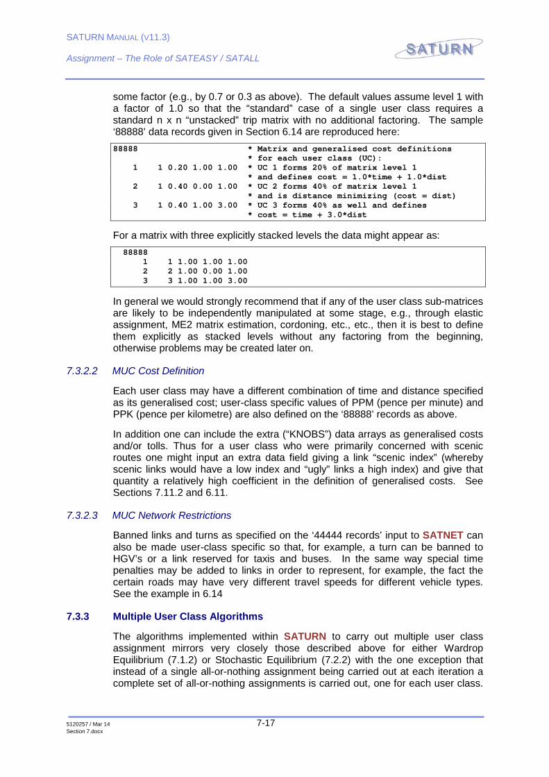
some factor (e.g., by 0.7 or 0.3 as above). The default values assume level 1 with a factor of 1.0 so that the “standard” case of a single user class requires a standard n x n “unstacked” trip matrix with no additional factoring. The sample ‘88888’ data records given in Section 6.14 are reproduced here: 88888 * Matrix and generalised cost definitions * for each user class (UC): 1 1 0.20 1.00 1.00 * UC 1 forms 20% of matrix level 1 * and defines cost = 1.0*time + 1.0*dist 2 1 0.40 0.00 1.00 * UC 2 forms 40% of matrix level 1 * and is distance minimizing (cost = dist) 3 1 0.40 1.00 3.00 * UC 3 forms 40% as well and defines * cost = time + 3.0*dist
For a matrix with three explicitly stacked levels the data might appear as: 88888 1 1 1.00 1.00 1.00 2 2 1.00 0.00 1.00 3 3 1.00 1.00 3.00
In general we would strongly recommend that if any of the user class sub-matrices are likely to be independently manipulated at some stage, e.g., through elastic assignment, ME2 matrix estimation, cordoning, etc., etc., then it is best to define them explicitly as stacked levels without any factoring from the beginning, otherwise problems may be created later on.
7.3.2.2 MUC Cost Definition
Each user class may have a different combination of time and distance specified as its generalised cost; user-class specific values of PPM (pence per minute) and PPK (pence per kilometre) are also defined on the ‘88888’ records as above.
In addition one can include the extra (“KNOBS”) data arrays as generalised costs and/or tolls. Thus for a user class who were primarily concerned with scenic routes one might input an extra data field giving a link “scenic index” (whereby scenic links would have a low index and “ugly” links a high index) and give that quantity a relatively high coefficient in the definition of generalised costs. See Sections 7.11.2 and 6.11.
7.3.2.3 MUC Network Restrictions
Banned links and turns as specified on the ‘44444 records’ input to SATNET can also be made user-class specific so that, for example, a turn can be banned to HGV’s or a link reserved for taxis and buses. In the same way special time penalties may be added to links in order to represent, for example, the fact the certain roads may have very different travel speeds for different vehicle types. See the example in 6.14
7.3.3 Multiple User Class Algorithms
The algorithms implemented within SATURN to carry out multiple user class assignment mirrors very closely those described above for either Wardrop Equilibrium (7.1.2) or Stochastic Equilibrium (7.2.2) with the one exception that instead of a single all-or-nothing assignment being carried out at each iteration a complete set of all-or-nothing assignments is carried out, one for each user class.
SATURN MANUAL (V11.3)
Assignment – The Role of SATEASY / SATALL
5120257 / Mar 14 7-18 Section 7.docx
Note that costs are therefore only updated AFTER all user classes have been re-assigned.
Thus in the Frank-Wolfe algorithm the combination of the old and auxiliary (all-or-nothing) flows is the same for all classes. Hence at the end of the algorithm the fraction of trips assigned to each iteration’s routes is identical across all classes. (There is one exception to this rule - if a user class is assigned to “fixed cost” routes, e.g., minimum distance, it is assigned once and only once to that route in iteration 1 and thereafter disregarded.)
Similarly with the Stochastic Multiple User Class Assignment the MSA algorithm assigns equal flows to each iteration over all classes. Note that the values of SUET may differ by user class as defined via subscripted values of SUET under &PARAM; e.g., SUET(2) = 0.5 defines SUET for user class 2 specifically, SUIET = 0.5 defines it for all user classes. See also 6.11.
7.4 Joint Equilibrium Assignment and Variable Demand Models
7.4.1 General Principles of Supply-Demand Equilibrium
Previous discussions have assumed that the trip matrix to be assigned is “fixed” independent of the road costs that emerge from the assignment process. A more general modelling approach is to assume that the road trip matrix (or matrices) depends on the (generalised) cost of travel; traditional model forms include, e.g., distribution or modal split models where the choice of destination and/or mode depends on the road (plus other) costs. We refer to these as “variable demand models” and we can write in very general terms
Equation 7.7
( )T d C=
where T is a general vector representing all o-d movements to be assigned and c represents all o-d costs (by road). Traditional 4-stage models fall into this category.
Equally the assignment procedure for a fixed trip matrix T may be thought of as a process, one output of which will be o-d travel costs by road. These costs will depend, via the levels of congestion, on the input trip matrix. We can therefore think of the assignment as a network “supply” or “performance” model and write:
Equation 7.8
( )C s T=
In such a joint modelling approach we require that the demand and supply processes are not only internally consistent but are also consistent between themselves such that, using * to denote joint equilibrium.
Equation 7.9 * *( )T d c= (a)
and * *( )c s T= (b)

SATURN MANUAL (V11.3)
Assignment – The Role of SATEASY / SATALL
5120257 / Mar 14 7-19 Section 7.docx
In other words, given a set of network travel costs c*, the demand model produces a set of trip matrix (road) demands T* and, if we assign T* to the road network, the resulting o-d travel costs are again c*. The demand and supply models are therefore in “equilibrium”.
The general form of the demand and supply models is as sketched in Figure 7.2 indicating that demand decreases as travel costs increase and that travel costs increase (congestion) as demand increases. The equilibrium we seek is at the intersection of the two curves.
Figure 7.2 - Supply/Demand Equilibrium
Figure 7.2 is of course highly simplified and in two dimensions; in “real” models both costs and trips are nzxnz matrices (with even further disaggregation possible by, e.g. user class or time period). However the general principle of an equilibrium intersection point still holds.
Note also in Figure 7.2 that a “fixed” trip matrix would correspond to a demand curve which would simply be a vertical line. Equally the nearer the demand curve (in this diagram) is to the horizontal the more sensitive are the demands to the costs (and, as we shall see below, the more difficult it is likely to be to solve for the joint equilibrium).
(Certain people may prefer to have costs along the X-axis and trips along the Y-axis and, indeed, when considering demand curves on their own, this is probably more natural. The concept of equilibrium holds either way; take your pick!)
In addition, provided we specify that the assignment or route choice must satisfy the Wardrop Equilibrium conditions (7.1.1), the resulting model may be thought of as being in “double equilibrium” such that both route and wider (e.g. whether to travel by road) choices are in equilibrium with the resulting road costs.

SATURN MANUAL (V11.3)
Assignment – The Role of SATEASY / SATALL
5120257 / Mar 14 7-20 Section 7.docx
SDM AND VDM MODELS: TERMINOLOGY
Demand models may be conveniently sub-divided into two categories:
♦ those where the number of trips by road for a specific ij movement Tij only depends on costs by road for that ij pair; and
♦ those where Tij depends (directly or indirectly) on all costs.
An example of 1) would be modal split where the choice between road and public transport for a single ij pair is a function only of the relative ij road and PT costs but the choice of destination is fixed. An example of 2) would be a constrained distribution model where, if the value of one Tij cell is reduced, then those trips will be re-assigned to another cell.
We may also describe these two categories as being “separable demand” or “non-separable demand” models in the sense that the cost-dependence in type 1) may be separated by ij cell but not with type 2). Alternatively one can speak of type 1) as an “own-cost” demand model. It has also become common to speak of type 1) demand models as being “simple”.
For both these reasons our current (post January 2006) preference is to use the shorthand abbreviations SDM and VDM to distinguish between types 1) and 2) models respectively: DM for “Demand Models”, S for either “Simple” or “Separable” and V for “Variable”.
Unfortunately there is a lot of alternative terminology for demand models in common circulation and some confusion is virtually inevitable, even within the SATURN Manual.
Thus originally SATURN allowed only for type 1) (SDM) models and these became widely known as either “elastic” or sometimes “SATEASY” models. However, on its own, elastic is not a particularly useful definition since (a) in a sense all demand models are elastic in that they allow the trip matrices to be “stretched”, and (b) there is a specific form of SDM known as Constant Elasticity (7.7.1). In addition elasticity is a standard and well-defined economic concept (7.7.5) which applies to all demand models. Despite these objections, and in deference to past common usage, the documentation will use the terms “elastic assignment” or “elastic equilibrium assignment” in addition to, or sometimes even instead of, SDM.
In general the internal “elastic assignment algorithms” available within SATURN apply only to separable demand models, although they have also been extended – primarily as a demonstration of a general principle - to one particular form of a variable demand model (singly constrained distribution; see Section 7.10). Thus Sections 7.5 to 7.9 refer only to SDM models. However SATURN may also be used in conjunction with a whole host of external VDM as described in Section 7.4.5.
The demand models available within SATURN generally require one or more “other” costs rather than simply the costs by road. For example a modal split model may need to have a matrix of ij costs by the public transport mode. Sometimes, as in the case of incremental demand models (7.8), these may be generated by other SATURN runs; however other times, as in the case of public

SATURN MANUAL (V11.3)
Assignment – The Role of SATEASY / SATALL
5120257 / Mar 14 7-21 Section 7.docx
transport cost matrices, these will need to be generated by other models and converted (as required) into SATURN matrix format.
We may also note at this point the general principles outlined above apply equally well to multiple user class assignment where, potentially at least, each user class may be modelled according to a different form of variable demand model or the same form but with different parameters. See 7.9 for detailed instructions.
7.4.2 Equivalent Optimisation Formulations: Separable Demand Models
Thus far we have only specified the solution to the joint assignment and variable demand problem as the point of intersection between (multi-dimensional) demand and supply curves as illustrated in Figure 7.2. However it turns out that, subject to certain restrictions on the properties of the supply and demand curves, the solution point also has the property that it minimises a certain convex function. This in fact simply extends the equivalence of Wardrop equilibrium assignment to a minimisation problem as discussed in Section 7.1.1.
In particular, the restrictions on the form of demand curves are most easily satisfied by separable demand functions although they may be further extended to certain – but definitely not all – forms of variable demand functions. In other words objective functions may be applied to SDM but not, in general, VDM.
The advantage of being able to represent joint assignment/demand problems as minimisation problems is that it enables strictly convergent solution algorithms to be developed, in the same way that the Frank-Wolfe algorithm (see 7.1.2) solves for Wardrop Equilibrium. In fact the algorithms used in SATURN for joint assignment/demand problems are basically extensions of the Frank-Wolfe algorithm.
In very general terms the combined objective function may be written as:
Equation 7.10
1
0 0( ) ( )
T TZ s t dt d t dt−= −∫ ∫
where d-1(T) represents the “inverse” demand curve; i.e. if T = d(c) then c = d-
1(T)*.
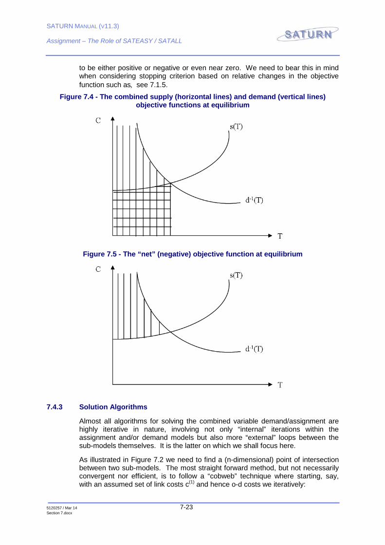
The first term in (7.10) is equivalent to the standard Wardrop Equilibrium objective function (7.1); the second term represents the negative of the “area” underneath the demand curve from 0 up to T. Both are illustrated individually in Figures 7.3a and 7.3b respectively and, as they would appear at the equilibrium, in Figure 7.4.
* Note that in our diagrams there is no difference between the curves d(c) and d-1(T); they differ only in terms of which variable or axis is thought of as being the “independent” variable.

SATURN MANUAL (V11.3)
Assignment – The Role of SATEASY / SATALL
5120257 / Mar 14 7-22 Section 7.docx
Figure 7.3 (a) - The supply-side objective function
(b) - The demand-side objective function
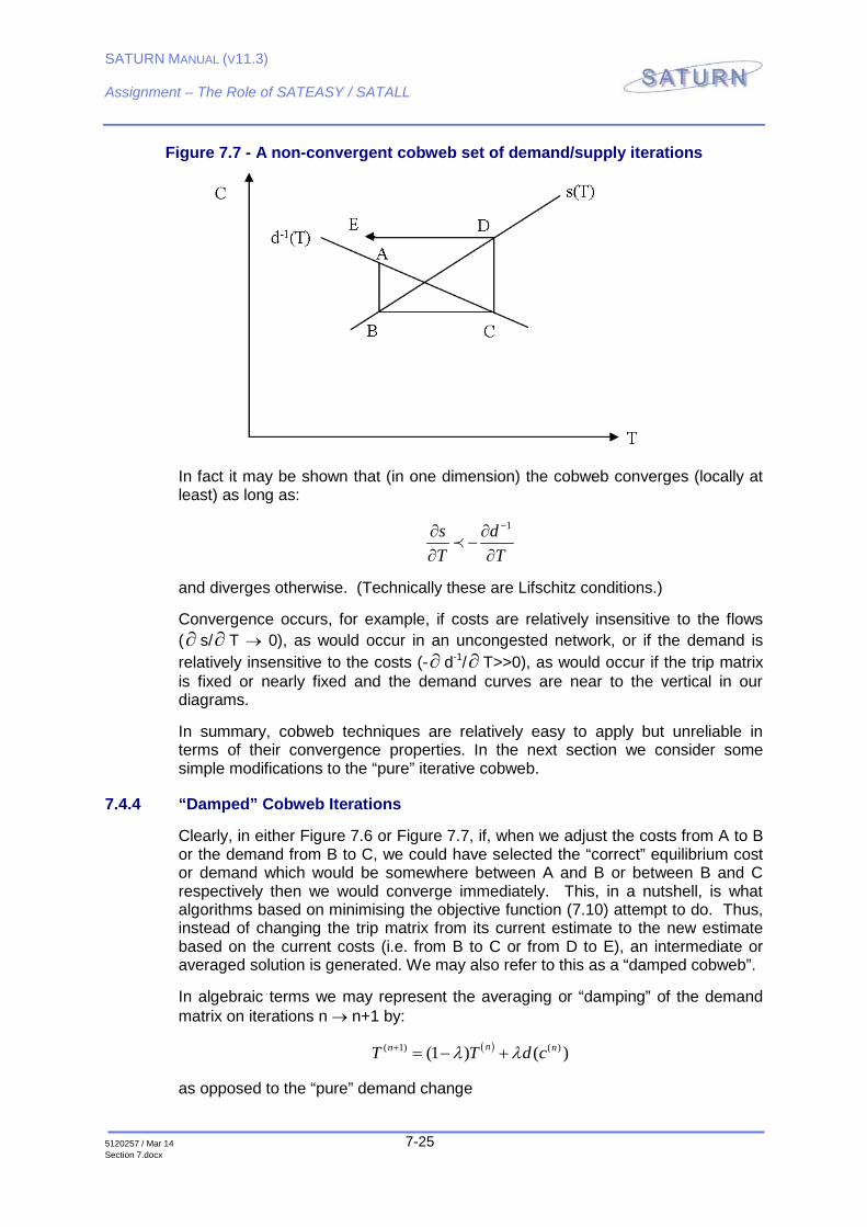
Note that in Figure 7.4 the area under the supply curve (represented by the horizontal hatching) is positive while that under the inverse demand curve (the vertical hatching) is negative. Hence at equilibrium the supply contribution is exactly “cancelled out” by part of the demand contribution, leaving a “net” negative contribution as illustrated in Figure 7.5.
Thus the problem of minimising the objective function (7.10) may be interpreted geometrically as making the negative area in Figure 7.5 as large - in absolute terms - as possible. Which, if you think about it long enough, implies taking T as the point of intersection in Figure 7.5. (The “negative” area keeps increasing as we go from 0 up to the point of intersection but if we go beyond the intersection point the negative contribution from the demand curve is now below the positive contribution from the supply curve - a bad thing from the point of view of minimisation.)
A further, somewhat technical, implication of having both positive and negative components in the objective function is that the final optimum value may turn out
SATURN MANUAL (V11.3)
Assignment – The Role of SATEASY / SATALL
5120257 / Mar 14 7-23 Section 7.docx
to be either positive or negative or even near zero. We need to bear this in mind when considering stopping criterion based on relative changes in the objective function such as, see 7.1.5.
Figure 7.4 - The combined supply (horizontal lines) and demand (vertical lines) objective functions at equilibrium
Figure 7.5 - The “net” (negative) objective function at equilibrium
7.4.3 Solution Algorithms
Almost all algorithms for solving the combined variable demand/assignment are highly iterative in nature, involving not only “internal” iterations within the assignment and/or demand models but also more “external” loops between the sub-models themselves. It is the latter on which we shall focus here.
As illustrated in Figure 7.2 we need to find a (n-dimensional) point of intersection between two sub-models. The most straight forward method, but not necessarily convergent nor efficient, is to follow a “cobweb” technique where starting, say, with an assumed set of link costs c(1) and hence o-d costs we iteratively:

SATURN MANUAL (V11.3)
Assignment – The Role of SATEASY / SATALL
5120257 / Mar 14 7-24 Section 7.docx
Solve for the corresponding trip matrix (demand)
Assign that trip matrix to the network to obtain a new set of link flows plus costs (supply) and return to step (1).
In more algebraic terms we may represent the process by:
( ) ( ) ( ) ( 1)n n n n nij ij a a ijC T V c c +→ → → → →
We could equally start the iterative process with an assumed trip matrix T(1) such that the first model carried out is supply (assignment), not demand.
However we start, the process may be terminated when (and if) the trip matrices (or cost matrices, link flows, etc) are sufficiently close on two successive iterations.
Diagrammatically, and in one dimension, the procedure is as illustrated in Figure 7.6 where, starting with assumed costs c(1) and the corresponding demand T(1) represented at point A, step (2) above (supply) is represented by the vertical line from A to B and step (1) (demand) by the horizontal line from B to C. Here successive applications of the supply and demand sub-models take us through successive points A, B, C, D, E, which spiral in towards the ultimate point of intersection - equilibrium.
Figure 7.6 - A (convergent) cobweb set of demand/supply iterations
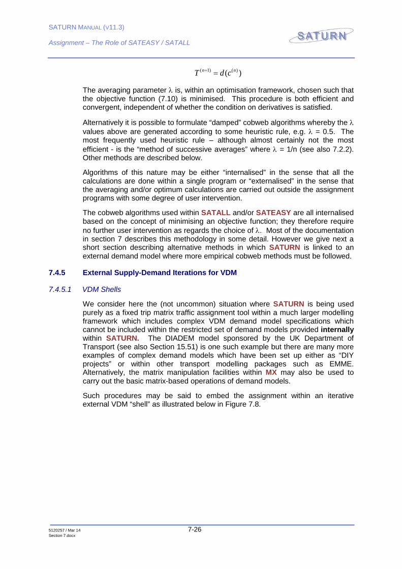
However convergence need not occur and the “cobweb” may spiral out in a non-convergent fashion just as easily as inwards, as illustrated in Figure 7.7.
SATURN MANUAL (V11.3)
Assignment – The Role of SATEASY / SATALL
5120257 / Mar 14 7-25 Section 7.docx
Figure 7.7 - A non-convergent cobweb set of demand/supply iterations
In fact it may be shown that (in one dimension) the cobweb converges (locally at least) as long as:
1s dT T
−∂ ∂−
∂ ∂
and diverges otherwise. (Technically these are Lifschitz conditions.)
Convergence occurs, for example, if costs are relatively insensitive to the flows (∂ s/∂ T → 0), as would occur in an uncongested network, or if the demand is relatively insensitive to the costs (-∂ d-1/∂ T>>0), as would occur if the trip matrix is fixed or nearly fixed and the demand curves are near to the vertical in our diagrams.
In summary, cobweb techniques are relatively easy to apply but unreliable in terms of their convergence properties. In the next section we consider some simple modifications to the “pure” iterative cobweb.
7.4.4 “Damped” Cobweb Iterations
Clearly, in either Figure 7.6 or Figure 7.7, if, when we adjust the costs from A to B or the demand from B to C, we could have selected the “correct” equilibrium cost or demand which would be somewhere between A and B or between B and C respectively then we would converge immediately. This, in a nutshell, is what algorithms based on minimising the objective function (7.10) attempt to do. Thus, instead of changing the trip matrix from its current estimate to the new estimate based on the current costs (i.e. from B to C or from D to E), an intermediate or averaged solution is generated. We may also refer to this as a “damped cobweb”.
In algebraic terms we may represent the averaging or “damping” of the demand matrix on iterations n → n+1 by:
( )( 1) ( )(1 ) ( )nn nT T d cλ λ+ = − +
as opposed to the “pure” demand change
SATURN MANUAL (V11.3)
Assignment – The Role of SATEASY / SATALL
5120257 / Mar 14 7-26 Section 7.docx
( 1) ( )( )n nT d c+ =
The averaging parameter λ is, within an optimisation framework, chosen such that the objective function (7.10) is minimised. This procedure is both efficient and convergent, independent of whether the condition on derivatives is satisfied.
Alternatively it is possible to formulate “damped” cobweb algorithms whereby the λ values above are generated according to some heuristic rule, e.g. λ = 0.5. The most frequently used heuristic rule – although almost certainly not the most efficient - is the “method of successive averages” where λ = 1/n (see also 7.2.2). Other methods are described below.
Algorithms of this nature may be either “internalised” in the sense that all the calculations are done within a single program or “externalised” in the sense that the averaging and/or optimum calculations are carried out outside the assignment programs with some degree of user intervention.
The cobweb algorithms used within SATALL and/or SATEASY are all internalised based on the concept of minimising an objective function; they therefore require no further user intervention as regards the choice of λ. Most of the documentation in section 7 describes this methodology in some detail. However we give next a short section describing alternative methods in which SATURN is linked to an external demand model where more empirical cobweb methods must be followed.
7.4.5 External Supply-Demand Iterations for VDM
7.4.5.1 VDM Shells
We consider here the (not uncommon) situation where SATURN is being used purely as a fixed trip matrix traffic assignment tool within a much larger modelling framework which includes complex VDM demand model specifications which cannot be included within the restricted set of demand models provided internally within SATURN. The DIADEM model sponsored by the UK Department of Transport (see also Section 15.51) is one such example but there are many more examples of complex demand models which have been set up either as “DIY projects” or within other transport modelling packages such as EMME. Alternatively, the matrix manipulation facilities within MX may also be used to carry out the basic matrix-based operations of demand models.
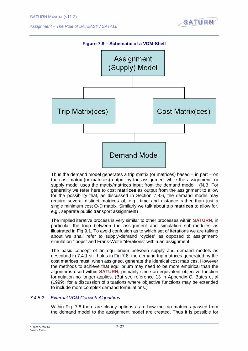
Such procedures may be said to embed the assignment within an iterative external VDM “shell” as illustrated below in Figure 7.8.
SATURN MANUAL (V11.3)
Assignment – The Role of SATEASY / SATALL
5120257 / Mar 14 7-27 Section 7.docx
Figure 7.8 – Schematic of a VDM-Shell
Thus the demand model generates a trip matrix (or matrices) based – in part – on the cost matrix (or matrices) output by the assignment while the assignment or supply model uses the matrix/matrices input from the demand model. (N.B. For generality we refer here to cost matrices as output from the assignment to allow for the possibility that, as discussed in Section 7.8.6, the demand model may require several distinct matrices of, e.g., time and distance rather than just a single minimum cost O-D matrix. Similarly we talk about trip matrices to allow for, e.g., separate public transport assignment)
The implied iterative process is very similar to other processes within SATURN, in particular the loop between the assignment and simulation sub-modules as illustrated in Fig 9.1. To avoid confusion as to which set of iterations we are talking about we shall refer to supply-demand “cycles” as opposed to assignment-simulation “loops” and Frank-Wolfe “iterations” within an assignment.
The basic concept of an equilibrium between supply and demand models as described in 7.4.1 still holds in Fig 7.8: the demand trip matrices generated by the cost matrices must, when assigned, generate the identical cost matrices. However the methods to achieve that equilibrium may need to be more empirical than the algorithms used within SATURN, primarily since an equivalent objective function formulation no longer applies. (But see reference 13 in Appendix C, Bates et al (1999), for a discussion of situations where objective functions may be extended to include more complex demand formulations.)
7.4.5.2 External VDM Cobweb Algorithms
Within Fig. 7.8 there are clearly options as to how the trip matrices passed from the demand model to the assignment model are created. Thus it is possible for
SATURN MANUAL (V11.3)
Assignment – The Role of SATEASY / SATALL
5120257 / Mar 14 7-28 Section 7.docx
users to set up their own versions of cobweb iterations (damped or otherwise) to define the latest trip matrices.
We have already described two very common “damped” cobweb algorithms; i.e., the straightforward “averaging method” where λ = 0.5 and the “method of successive averages” where λ = 1/n (see also 7.2.2). There are, however, several alternative strategies which have been proposed over the years, the objective of all of them being to achieve an acceptable degree of equilibrium in the shortest possible time.
Thus the simplest method is not to damp the cobweb iterations at all so that, in effect, λ = 1.0. Empirically this method appears to be most successful if the demand model is relatively insensitive to assignment costs (low elasticity).
DIADEM uses a method known as “Algorithm 1” which basically starts with an initial arbitrary value of λ , e.g., 0.5, and continues with the same value as long as an “objective function” (a measure of convergence) continues to decrease. If, however, the gap increases the value of λ is halved until a decrease in the gap is obtained. For further details we refer you to the DIADEM Manual. The convergence properties of Algorithm 1 with realistic demand and supply models is a subject of some debate but there is evidence that beyond a certain point it tends to “stick”.
Another technique is the “Fixed Step Length” Algorithm (FSL) whereby, as the name suggests, an initial value is set for λ and that value fixed throughout all supply-demand iterations. Thus the averaging method where λ = 0.5 and the pure cobweb where λ = 1.0 are both examples of FSL. It has been shown by Hillel BarGera and Dave Boyce (Solving a non-convex combined travel forecasting model by the Method of Successive Averages with constant step sizes, Transportation Research Part B, 40, 5, 351-367, (2006).) that FSL is guaranteed to converge as long as a small enough value of λ is set.
Empirical work by DVV has suggested a formula λ = 1.0 / (1.0 + Ɛ) where Ɛ is a global measure of elasticity in the demand model.
7.4.5.3 Reducing CPU time: “Relaxed” SATALL Convergence Criteria
One of the problems associated with external VDM models as opposed to combined assignment-demand models based on minimising an objective function is that the extra series of cycles between the demand model and the assignment model inevitably leads to increased CPU time, generally – but not always – due to the time taken by the assignment model.
One obvious answer to this problem is to minimise the number of external cycles by designing a “clever” cobweb algorithm but this is somewhat outside the scope of SATURN.
An alternative strategy to reduce total CPU time, which does involve SATURN, is to recognise that there is very little point carrying out a very highly convergent and accurate assignment within SATALL using a particular trip matrix if that trip matrix is going to be significantly altered by the next cycle of the demand model. This suggests that one should try to set easy (relaxed) assignment convergence criteria for early loops of the demand-supply cycle but to tighten the convergence

SATURN MANUAL (V11.3)
Assignment – The Role of SATEASY / SATALL
5120257 / Mar 14 7-29 Section 7.docx
criteria for the assignment as the overall convergence improves. (The same basic idea is applied to the simulation-assignment loops within SATALL by using the AUTONA option to set variable values of NITA dependent upon the overall gap value; see Section 9.5.4).
Thus parameters such as MASL, ISTOP etc. etc. which control the overall assignment-simulation convergence of a run of SATALL may need to be reset by the cobweb “driver” at each repeated run of SATURN, as indeed may parameters such as NITA which control the convergence of the assignment. There may be a good case here for using KONSTP = 1 and setting a critical Gap value in STPGAP as determined by the latest gap value achieved by the demand model.
The decision as to which parameters and how to select ”optimum” values is up to the user, being essentially external to SATURN. In terms of a “mechanism” for inputting those values into a new run of SATURN there are several possibilities. For example, they could defined within a $INCLUDE file within &PARAM which the controlling program could overwrite. Equally they could be set in a control file for SATALL.
In a similar vein it may be possible to simplify each intermediate run of SATALL by excluding certain options that are only required once the final trip matrix has been obtained. For example, the SAVEIT option may only be necessary on the final run (unless – see below – you are using WSTART).
Clearly best practice will only become clearer after considerable experimentation. One example of such experimentation is the CASSINI program described in 15.54.
USING UPDATE AND WSTART WITH VDM
One should also note that making the maximum use of facilities such as update and warm starts at every re-run of a SATURN assignment is strongly recommended in order to reduce run times, particularly when changes in the trip matrix from one external cycle to the next are relatively small. See sections 22.5.5 and 22.6.
However we strongly advise that warm starts should only be undertaken in conjunction with OBA due to the extra overheads incurred by Frank-Wolfe to carry out the extra SAVEIT assignment at the end of one cycle and the initial re-assignment at the start of the next assignment cycle.
7.4.6 The Final Trip Matrix and Routes
At the end of a variable demand assignment a final estimate of the road trip matrix Tij will have been obtained and assigned to give link flows Va. The link flows are stored on the output .ufs file in the normal way and the trip matrix is output as a separate .ufm file (see 7.12.1 and 7.12.3). The total number of trips within that matrix are reported both within the lp files and also saved within the output .ufs file where they may be printed via SATLOOK output options (11.11.4 and 17.9).
With respect to the output trip O-D file we note that any intra-zonal trips in the input trip matrix are neither assigned nor subject to demand calculations. Essentially therefore their output values are indeterminate. However, in order to avoid losing them entirely, the input intra-zonal values are (post SATURN 10.4)

SATURN MANUAL (V11.3)
Assignment – The Role of SATEASY / SATALL
5120257 / Mar 14 7-30 Section 7.docx
copied directly to the output trip matrix file. Similar considerations may also apply to inter-zonal cells which, for one reason or another, are unconnected; see 7.5.7.
Unlike the normal fixed trip matrix procedures, elastic assignment does not (for various technical reasons) record any information on the precise routes used to relate Va to Tij as normally saved if SAVEIT = T.
However, in the case of VDM/elastic assignments, the routes may be estimated by carrying out a final fixed trip matrix assignment using standard algorithms and recording the routes used via a .ufc file (see 15.23). It is these routes and the output trip matrix Tij which will be used in any post-assignment analyses, e.g. select link analysis (11.8.1).
We may further note, as discussed further in 15.23, that the routes found in this manner will not be 100% identical to those implied by the original elastic assignment, nor equally will the flows produced in the final assignment be identical to Va (although a very good approximation). It is therefore the Va obtained from the elastic assignment which are retained as the “correct” link flows.
Finally we note, as also mentioned in 15.23, that the number of assignment iterations used to calculate the final routes, strictly speaking NITA_S, may be different from the number used in the assignments proper, NITA. Thus, and in particular if you have set a relatively small value of NITA in order to reduce overall cpu time, a better estimate of the final routes should be obtained by defining NITA_S > NITA.
7.4.7 Further Recommended Reading
The notes given in this manual are not intended as a fully comprehensive guide to either simple or variable demand modelling and users who wish to carry out such modelling steps are strongly advised to read more widely. For general information see, for example, “Modelling Transport” by J. de D. Ortuzar and L.G. Willumsen, John Wiley and Sons. For a much more detailed analysis with particular reference to logit models try Norbert Oppenhem’s “Urban Travel Demand Modelling”, also John Wiley and Sons.
UK-based modellers may wish to refer to advice available on-line via WebTAG: www.dft.gov.uk/webtag.
7.5 SDM Assignment:
7.5.1 General Principles
We consider here the restricted or simple form of variable demand assignment, to be referred to as “elastic” or SDM assignment, where the number of (vehicle) trips from origin i to destination j is a ‘demand’ function of the cost (i.e., generalised time) of (vehicle) travel between i and j only; hence:
Equation 7.11
( )ij ijT f c=
This demand form corresponds most closely with a modal split model whereby ij trips are selecting either road or public transport modes but the destination is
SATURN MANUAL (V11.3)
Assignment – The Role of SATEASY / SATALL
5120257 / Mar 14 7-31 Section 7.docx
fixed. However, it could also be thought of as representing the decision as to when to travel (departure time choice), whether to travel or not (frequency) or whether to go as a passenger (occupancy). It does not, for example, fit into a model of trip distribution where the choice of whether to travel from i to j is a function of the costs to ALL destinations.
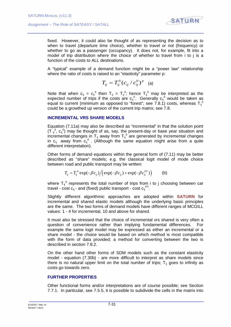
A “typical” example of a demand function might be a “power law” relationship where the ratio of costs is raised to an "elasticity" parameter p:
0 0( / ) pij ij ij ijT T c c= (a)
Note that when cij = cij0 then Tij = Tij
0; hence Tij0 may be interpreted as the
expected number of trips if the costs are cij0. Generally cij
0 would be taken as equal to current (minimum as opposed to “forest”; see 7.8.1) costs, whereas Tij
0 could be a growthed up version of the current trip matrix; see 7.8.
INCREMENTAL VRS SHARE MODELS
Equation (7.11a) may also be described as “incremental” in that the solution point (T ij
0, cij0) may be thought of as, say, the present-day or base year situation and
incremental changes in Tij away from Tij0 are generated by incremental changes
in cij away from cij0 . (Although the same equation might arise from a quite
different interpretation).
Other forms of demand equations within the general form of (7.11) may be better described as “share” models; e.g. the classical logit model of mode choice between road and public transport may be written:
( )exp( ) exp( ) exp( )A PTij ij ij ij ijT T c c cβ β β= − − + − (b)
where TijA represents the total number of trips from i to j choosing between car
travel - cost cij - and (fixed) public transport - cost cijPT.
Slightly different algorithmic approaches are adopted within SATURN for incremental and shared elastic models although the underlying basic principles are the same. The two forms of demand models have different ranges of MCGILL values: 1 - 4 for incremental, 10 and above for shared.
It must also be stressed that the choice of incremental vrs shared is very often a question of convenience rather than implying fundamental differences. For example the same logit model may be expressed as either an incremental or a share model - the choice would be based on which method is most compatible with the form of data provided; a method for converting between the two is described in section 7.8.2.
On the other hand other forms of SDM models such as the constant elasticity model - equation (7.30b) - are more difficult to interpret as share models since there is no natural upper limit on the total number of trips; Tij goes to infinity as costs go towards zero.
FURTHER PROPERTIES
Other functional forms and/or interpretations are of course possible; see Section 7.7.1. In particular, see 7.5.5, it is possible to subdivide the cells in the matrix into

SATURN MANUAL (V11.3)
Assignment – The Role of SATEASY / SATALL
5120257 / Mar 14 7-32 Section 7.docx
those that obey the elastic demand equation and those that are fixed independent of the cost. The latter cells are termed either “inelastic” or “frozen”.
As mentioned in 7.4 the problem in elastic equilibrium assignment is to determine both a self-consistent set of route choices and demand choices.
Elastic assignment is of most use in the assessment of future year networks where, say, a simple extrapolation of the current trip matrix leads to an extremely congested network with extremely high travel costs. Elastic assignment provides a method for keeping the trip matrix - the demand - within behaviourally realistic limits.
The elastic assignment algorithms within SATURN were developed as a joint project between the Institute for Transport Studies and WS Atkins, funded by DTp and administered by TRL. The reports produced for this study provide a comprehensive review of theory, algorithms and applications; copies are available from DVV.
7.5.2 Solution Algorithms
This section describes the specific algorithms used by the SATURN programs SATEASY and SATALL. Both incremental and share models are based on the general principle of minimising an objective function as outlined in Section 7.4.2 and the iterative structure of 7.4.3. The precise details differ slightly between both; see 7.5.4.
7.5.2.1 Excess Trip (Pseudo Link) Algorithms
For incremental models it essentially follows the “excess trip” formulation, but with one or two new wrinkles introduced. Thus for every ij pair in the network an additional “pseudo” link is introduced in order to carry the traffic that is excess to the road network. This is illustrated in Figure 7.8.
Figure 7.9 - The “Pseudo Link” Representation of Elastic Assignment
For each origin-destination pair ij the maximum number of trips that might possibly use the road network, Tij
max, is calculated (see 7.5.3.1). These trips may then choose either to travel through the "real" network or via the ij - specific “pseudo” link. We denote these flows by Tij and Eij respectively. Hence Tij will become the "actual" road trip matrix (although, in the algorithms used by SATURN, Tij is not explicitly stored but may be calculated, when needed, as Tij
max - Eij).
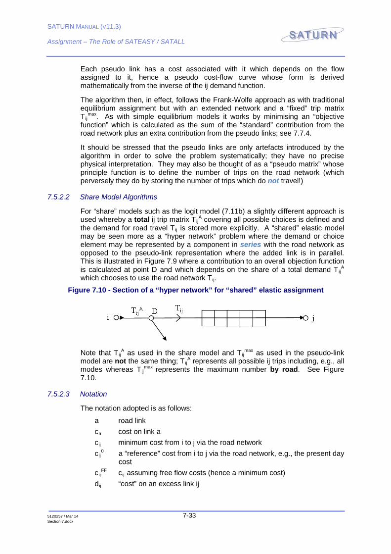
SATURN MANUAL (V11.3)
Assignment – The Role of SATEASY / SATALL
5120257 / Mar 14 7-33 Section 7.docx
Each pseudo link has a cost associated with it which depends on the flow assigned to it, hence a pseudo cost-flow curve whose form is derived mathematically from the inverse of the ij demand function.
The algorithm then, in effect, follows the Frank-Wolfe approach as with traditional equilibrium assignment but with an extended network and a “fixed” trip matrix Tij
max. As with simple equilibrium models it works by minimising an “objective function” which is calculated as the sum of the “standard” contribution from the road network plus an extra contribution from the pseudo links; see 7.7.4.
It should be stressed that the pseudo links are only artefacts introduced by the algorithm in order to solve the problem systematically; they have no precise physical interpretation. They may also be thought of as a “pseudo matrix” whose principle function is to define the number of trips on the road network (which perversely they do by storing the number of trips which do not travel!)
7.5.2.2 Share Model Algorithms
For “share” models such as the logit model (7.11b) a slightly different approach is used whereby a total ij trip matrix Tij
A covering all possible choices is defined and the demand for road travel Tij is stored more explicitly. A “shared” elastic model may be seen more as a “hyper network” problem where the demand or choice element may be represented by a component in series with the road network as opposed to the pseudo-link representation where the added link is in parallel. This is illustrated in Figure 7.9 where a contribution to an overall objection function is calculated at point D and which depends on the share of a total demand Tij
A which chooses to use the road network Tij.
Figure 7.10 - Section of a “hyper network” for “shared” elastic assignment
Note that TijA as used in the share model and Tij
max as used in the pseudo-link model are not the same thing; Tij
A represents all possible ij trips including, e.g., all modes whereas Tij
max represents the maximum number by road. See Figure 7.10.
7.5.2.3 Notation
The notation adopted is as follows:
a road link ca cost on link a cij minimum cost from i to j via the road network cij
0 a “reference” cost from i to j via the road network, e.g., the present day cost
cijFF cij assuming free flow costs (hence a minimum cost)
dij “cost” on an excess link ij
SATURN MANUAL (V11.3)
Assignment – The Role of SATEASY / SATALL
5120257 / Mar 14 7-34 Section 7.docx
Eij “Excess” or “Pseudo” flow from i to j Fij Excess flow from i to j (auxiliary solution) fij elastic demand function expressing trips as a function of costs
Tij = f ij (cij) gij the inverse of fij:
cij = gij(Tij) ij pseudo link connecting origin i to destination j Tij road trips from i to j Tij
o input “reference” trip matrix as used in the demand function Tij
max maximum possible trips from i to j; hence the “fixed” trip matrix to be assigned
Va flow on link a (averaged)
Wa flow on link a (auxiliary solution)
7.5.2.4 The Basic Pseudo Link Algorithm
We describe here the “pseudo link” algorithm as applied to incremental elastic demand models explicitly. The variations necessary to deal with share models are given in 7.5.4.
Step 1 Set all link costs to their free flow values and the iteration counter n = 1. For each origin i:
1a) Calculate the minimum cost tree to each destination j; cijFF represents
the minimum cost to j.
1b) For each destination j determine the maximum number of road trips possible for that ij pair by solving:
Equation 7.12 max ( )FF
ij ij ijT f c=
1c) Determine the number of trips to be loaded onto the road network: (1)
ijT
1d) Load Tij(1) onto the road network, accumulating the total link flows to
obtain the first set of road flows, Va(1).
1e) ‘Load’ the excess flow:
(1) max (1)ij ij ijE T T= −
onto the excess link
ITERATIVE LOOPS
Step 2 Calculate the ‘current’ link and pseudo link costs:

SATURN MANUAL (V11.3)
Assignment – The Role of SATEASY / SATALL
5120257 / Mar 14 7-35 Section 7.docx
Equation 7.13 ( ) ( )( )n na a ac c V= (a)
( ) max ( )( )n nij ij ij ijd g T E= − (b)
Step 3 For each origin i:
3a) Calculate the minimum cost tree to each destination j - costs cij(n).
3b) Calculate and load the auxiliary road trips for this iteration: ( 1)nijT + to
obtain link flows ( 1)naW +
3c) and load the remaining flow
( 1) max ( 1)n nij ij ijF T T+ += −
onto the pseudo link
Step 4 Combine the previous ‘solution’ flows with the ‘auxiliary’ flows found in Step 3 according to the equations:
Equation 7.14 ( 1) ( ) ( 1)(1 )n n n
a a aV V Wλ λ+ += − + (a)
( 1) ( ) ( 1)(1 )n n nij ij ijE E Fλ λ+ += − + (b)
where λ is chosen to minimise the objective function Z(λ).
Step 5 Check for convergence; if not reached increment the iteration counter and return to Step 2; else, stop.
7.5.3 Variations on the Basic Pseudo Link Algorithm
Each note refers to a particular step, or sub-step, in the algorithm 7.5.2.2:
7.5.3.1 The Maximum Number of ij Trips; 1b)
Tijmax represents the maximum possible number of ij trips which will use the road
network and, from this point on, the algorithm may be viewed as a standard assignment of a fixed trip matrix - Tij
max - to a network which includes an extra “pseudo” link for each ij pair.
Since Tij is a decreasing function of cij, and the costs can never be less than their free flow values cij
FF (assuming non-decreasing cost-flow curves) fij (cijmin) with
cijmin = cij
FF must be an upper bound.
By “maximum” we refer specifically to the maximum number of ij trips which could ever occur on the road, not to be confused with the maximum number of trips over all modes, say, or the intercept of the demand curve with the c=0 vertical axis. The different definitions of trips are illustrated in Figure 7.10 following
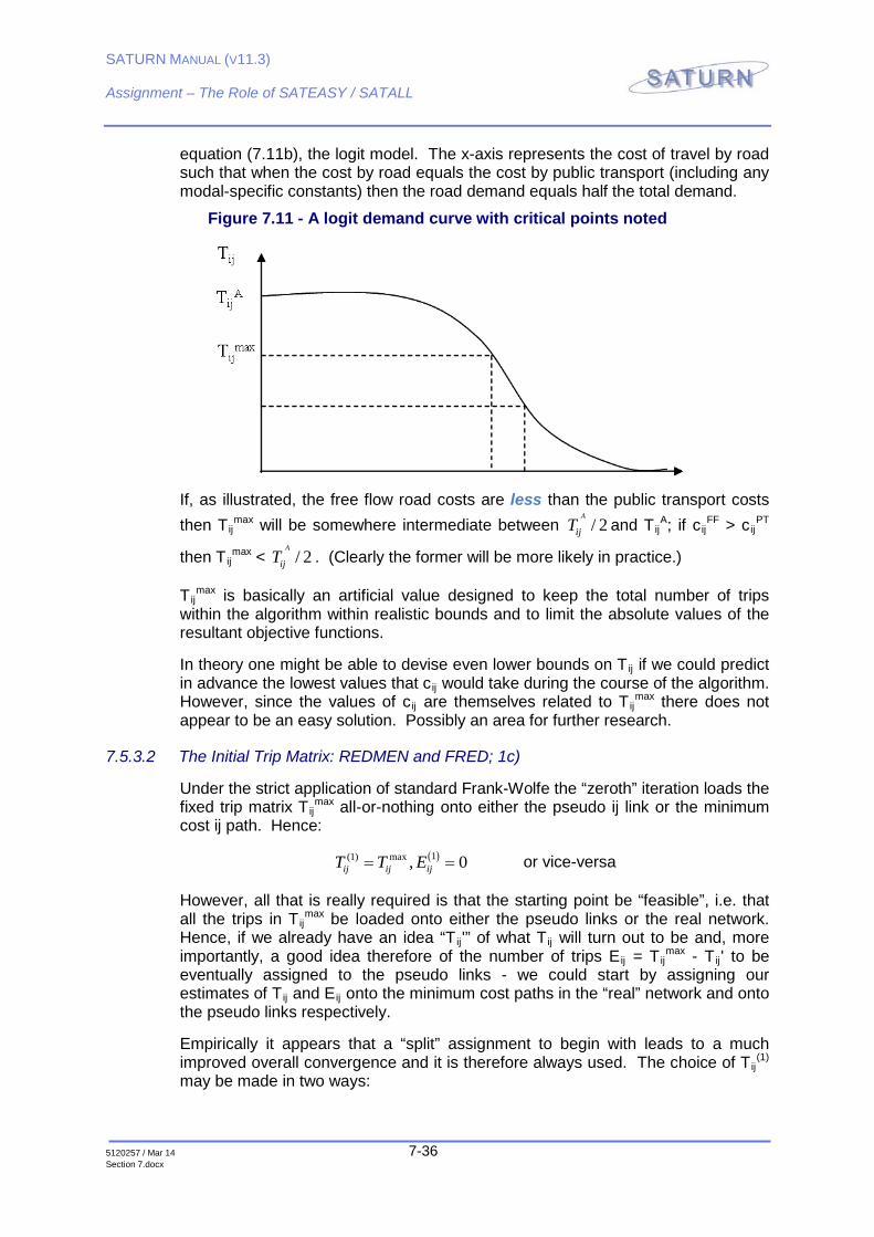
SATURN MANUAL (V11.3)
Assignment – The Role of SATEASY / SATALL
5120257 / Mar 14 7-36 Section 7.docx
equation (7.11b), the logit model. The x-axis represents the cost of travel by road such that when the cost by road equals the cost by public transport (including any modal-specific constants) then the road demand equals half the total demand.
Figure 7.11 - A logit demand curve with critical points noted
If, as illustrated, the free flow road costs are less than the public transport costs then Tij
max will be somewhere intermediate between / 2A
ijT and TijA; if cij
FF > cijPT
then Tijmax < / 2
A
ijT . (Clearly the former will be more likely in practice.)
Tijmax is basically an artificial value designed to keep the total number of trips
within the algorithm within realistic bounds and to limit the absolute values of the resultant objective functions.
In theory one might be able to devise even lower bounds on Tij if we could predict in advance the lowest values that cij would take during the course of the algorithm. However, since the values of cij are themselves related to Tij
max there does not appear to be an easy solution. Possibly an area for further research.
7.5.3.2 The Initial Trip Matrix: REDMEN and FRED; 1c)
Under the strict application of standard Frank-Wolfe the “zeroth” iteration loads the fixed trip matrix Tij
max all-or-nothing onto either the pseudo ij link or the minimum cost ij path. Hence:
( )1(1) max , 0ij ij ijT T E= = or vice-versa
However, all that is really required is that the starting point be “feasible”, i.e. that all the trips in Tij
max be loaded onto either the pseudo links or the real network. Hence, if we already have an idea “Tij'” of what Tij will turn out to be and, more importantly, a good idea therefore of the number of trips Eij = Tij
max - Tij' to be eventually assigned to the pseudo links - we could start by assigning our estimates of Tij and Eij onto the minimum cost paths in the “real” network and onto the pseudo links respectively.
Empirically it appears that a “split” assignment to begin with leads to a much improved overall convergence and it is therefore always used. The choice of Tij
(1) may be made in two ways:

SATURN MANUAL (V11.3)
Assignment – The Role of SATEASY / SATALL
5120257 / Mar 14 7-37 Section 7.docx
If REDMEN = T then it is taken from an input trip matrix which represents a prior estimate of Tij, for example from a previous assignment. The estimated trip matrix may be defined by the Namelist parameter FILRED under &PARAM in the network .dat file.
Otherwise (for incremental models only) it is set from the equation:
(1) 0.ij ijT T FRED=
where T0 represents the ‘inelastic’ or ‘reference’ trip matrix as used in the demand function - see 7.7.1, equations (7.30a) to (7.30d).
If REDMEN = T it must be stressed that the input trip matrix (FILRED) need only be an estimate but that the closer it is to the eventual output trip matrix, the better. Equally if it is a very poor estimate there must come a point where using this option turns out to be counter-productive. However, to date we have no empirical evidence to suggest where the cut off point comes. Note that, in this context, REDMEN may be regarded as a form of “kick start”; see 22.2.4.
N.B. See 7.5.6 for advice on using the REDMEN option in conjunction with “frozen” cells (ICING = T).
If REDMEN = F then FRED is a uniform factor chosen to estimate the expected growth or reduction (but usually the latter) in the final trip matrix relative to the inelastic trip matrix. For example if you think elastic effects remove 5% of the trips in T0
ij from the network then set FRED = 0.95. The default value of FRED is 1.0.
N.B. FRED is applied to incremental models only (MCGILL < 10).
Our advice would be, if feasible, to set REDMEN = T and to define an input matrix FILRED; FRED would be a second choice.
7.5.3.3 Pseudo Link Costs; 2)
The calculation of the link costs ca follows the standard formulae as determined by the flow-delay curves (user-set for buffer link, simulated for simulation turns) while the pseudo link costs are related to the definition of the elastic demand function. The functional forms for the 4 equations as used in SATURN are given in 7.7.3.
Note the pseudo link costs, as with all other costs used within elastic assignment, are generalised costs and that furthermore they are expressed in units of generalised time seconds.
7.5.3.4 The Iterative Road Trip Matrix: NITA_F and MASL_F; 3b)
Similar considerations to those given under 1c) apply here as well. Thus a “strict” interpretation of Frank-Wolfe rules would lead to an all-or-nothing situation:
Equation 7.15
( )( ) ( )
( ) ( )
max1
0
n nij ij ijn
ij n nij ij
T c dT
c d+
⟨= ⟩

SATURN MANUAL (V11.3)
Assignment – The Role of SATEASY / SATALL
5120257 / Mar 14 7-38 Section 7.docx
( )( ) ( )
( ) ( )1
max
0 n nij ijn
ij n nij ij ij
c dF
T c d+
⟨= ⟩
Hence the maximum number of trips is assigned to either the pseudo link or to the road network minimum cost route.
However, the pseudo/road split may be substantially relaxed by recognising that the underlying principle of Frank-Wolfe is to increase the flow on the current cheapest route. Hence, if the pseudo route is currently cheapest, i.e.,
Equation 7.16 ( ) ( )n nij ijc d> (a)
then we require more trips on the pseudo link: ( 1) ( )n n
ij ijF E+ > (b)
and fewer trips on the network proper:
( 1) ( )n nij ijT T+ < (c)
with the converse being true if the pseudo route is more expensive.
We can in fact guarantee that this condition is satisfied by setting
( 1) ( )n nij ij ijT f c+ = (d)
i.e. set the road trips equal to the equilibrium demand corresponding to the current minimum road costs. Thus:
( 1) max ( 1)n nij ij ijF T T+ += − (e)
That equation (7.16d) guarantees (7.16c) may be seen by reference to the fact that by definition the current road trips Tij
(n) and the current pseudo link costs are “in equilibrium” in the sense that:
( )( )n nij ij ijT f d= (f)
Thus, since Tij is a decreasing function of cij, (7.16c) must hold if (7.16a) holds.
Two further parameters, NITA F and MASL F, extend the concept of a “good” initial estimate of the trip matrix by retaining:
( ) (1)nij ijT T=
(i) for assignment iterations n = 1 up to and including NITA_F.
for all assignment iterations for assignment-simulation loops 1 through MASL_F.
Both options are still experimental but early indications are that a judicious choice of one or both variables may improve convergence rates. By default neither option is invoked although we would recommend their judicious use.

SATURN MANUAL (V11.3)
Assignment – The Role of SATEASY / SATALL
5120257 / Mar 14 7-39 Section 7.docx
OPTIMUM STEP LENGTH; 4)
In order to choose the optimum value of λ one may either use a routine which explicitly minimises Z as a one-dimensional function of λ or - much more conveniently - one may use a routine to find the “root” of the equation:
Equation 7.17
0=λddZ
(The identical 2 options occur with the Frank-Wolfe inelastic assignment algorithm). The equation for the derivative of Z with respect to λ may be written:
Equation 7.18
( 1) ( ) ( 1) ( )( )( ) ( )( )n n n nc a a ij ij ij
a ij
dZ C W V d F Ed
λ λλ
+ += − + −∑ ∑
where:
( ) ( )( )( 1)(1 ) n na a a ac c V Wλ λ λ += − + (a)
And
( 1)( ) (1 ) n nij ij ij ijd d E Fλ λ λ += − + (b)
Functional forms for dij ( ) are given in 7.7.3; ca ( ) are the cost-flow curves as defined by the user (or calculated by the simulation) for links in the road network.
7.5.4 Variations under Shared Demand Algorithms
The main difference between the algorithm used for incremental and share-based demand functions is that the former explicitly defines pseudo links and pseudo link flows which, in effect, define the current road trip matrix by subtraction from Tij
max whereas, with share-based functions, the road trip matrix and any other trip matrices involved are stored directly.
In both cases the trip matrices assigned to the roads at iteration n corresponds to the matrix consistent with the current o-d costs - equation (7.16d). The optimum lambda value at each step follows the same principle of minimising an objective function. Whereas the pseudo-link flows are averaged, equation (7.14b), the share algorithms average trip matrices directly.
The parameters REDMEN, NITA_F, MASL_F, etc. described in 7.5.3.2 and 7.5.3.4 apply to both approaches. On the other hand FRED applies only to incremental demand models.
7.5.5 Convergence Measures and Stopping Criteria
Convergence of the elastic algorithm may be monitored in precisely the same manner as with the inelastic Frank-Wolfe (with the obvious proviso that any summations over links must also include pseudo links). In addition a number of other measures may be formulated which refer more specifically to either road or pseudo links.

SATURN MANUAL (V11.3)
Assignment – The Role of SATEASY / SATALL
5120257 / Mar 14 7-40 Section 7.docx
The order of the parameters, and their abbreviations, given below corresponds to the columns in the elastic summary tables.
♦ The “normalised gap or delta function” as defined in 7.1.4 for inelastic Wardrop Equilibrium and here extended to include pseudo links. The gap G is the difference between current and minimum costs BEFORE division by the total cost; DELTA is normalised by dividing by total cost.
♦ The uncertainty in the objective function ‘ε‘, “EPS” in the LP tables. See equation (7.5), 7.1.5.
♦ The objective function Z (including pseudo links).
♦ FDZ, the percentage improvement in Z per iteration relative to Z.
♦ FIMP, the % improvement in Z relative to the uncertainty in the objective function.
♦ Total road/pseudo trips
♦ A necessary condition for convergence is that the total number of trips on the “real” network and the total number on the “pseudo” network reach stable values - although clearly this is not a sufficient condition since changes in individual ij values may be masked by an apparent stability of the total.
♦ DELTA-R, the delta function as evaluated only for trips through the real network and therefore a measure of how near the current path flows are to Wardrop Equilibrium (and therefore ignoring how near they are to demand equilibrium).
♦ TIJ-AAD - the average absolute difference between the current road trips and the number given by the demand function for the current costs, i.e.:
Equation 7.19 ( )( )n n
ij ij ijij
T f c−∑
♦ This is normalised by dividing by the total number of trips and expressed as a percentage. It therefore monitors “demand equilibrium”.
♦ TIJ-AD - as 8) but with actual differences, not absolute differences.
♦ TxCij-AAD – as 8) but with each ij element weighted by its cost and then normalised by the total vehicle-costs. (N.B. This is the equivalent of the “%Gap” as used in the demand-supply equilibration program DIADEM.)
♦ Total travel cost over the real road network expressed in veh-hrs.
At convergence measures 1), 2), 4), 5), 7), 8), 9) and 10) should all tend to zero.
Stopping criteria are based on the same criteria as those for Wardrop Equilibrium with a fixed trip matrix as listed in 7.1.5. Thus the user-set parameters NITA, XFSTOP, FISTOP and UNCRTS all apply.

SATURN MANUAL (V11.3)
Assignment – The Role of SATEASY / SATALL
5120257 / Mar 14 7-41 Section 7.docx
Note that all these convergence measures are internal to the assignment; i.e., they do not take into account any changes in costs introduced by the assignment-simulation loops as within SATALL. For convergence of the loops please refer to Section 9.9.1.
It is noted that to achieve satisfactory convergence of an elastic assignment often requires many more iterations than an inelastic one; rather higher values of NITA may therefore need to be used.
7.5.6 Frozen or Inelastic Trip Cells
A common problem in elastic assignment is that, if the network has been ‘cordoned’ at its outer boundaries, the ‘external trips’ which enter or leave at the cordon points will experience large proportions of their actual travel costs outside the network being modelled. This creates problems in using a single demand function for both internal and external trips. One solution is to divide the matrix up into two or more ‘user classes’ and define different functional forms and/or parameters for each; see 7.9.
A simpler solution is to “freeze” certain cells within the trip matrix, e.g. external trips, such that for those cells the trips are fixed according to:
0ij ijT T=
and are therefore, in effect, inelastic.
Frozen trips are defined by an input .ufm matrix where a cell value of 0 implies that that cell is inelastic or frozen and any non-zero value (1.0 recommended) implies that it is elastic.
N.B. In former versions of the documentation the definition of frozen/unfrozen cell values was wrong and the 0’s and 1’s were reversed. Please check that if you are using an “old” matrix to set frozen zones that the correct definition is being used.
To invoke the frozen cells option you must (a) set the parameter ICING to true and (b) define the frozen cell matrix (FILICE - see 7.12.3). Both may be most conventionally done using &PARAM namelist input in the network .dat file.
Alternatively (and this is not highly recommended) the frozen cell matrix may be set using the FREEZE option in the SATALL batch file (9.13). If both FILICE and FREEZE are used (definitely not recommended!) then the file set by FREEZE takes precedence.
If there are multiple user classes (NOMADS > 1) then the frozen cell matrix must have the same stacking levels as all the other matrices, i.e., the parametric trip matrix FILTIJ, the cost matrix FILCIJ, etc. etc.
We note that the frozen cell option may be applied to both incremental and shared demand models, although in the latter case we recommend caution. Thus in a shared model the output cell value Tij is set equal to the input trip matrix value Tij
0 for frozen cells whereas for the un-frozen cells Tij0 is “shared” between the
output Tij and the “other” choices; hence Tij0 potentially has two roles – car trips
and total trips - and it may be easy for the user to confuse the two. An alternative
SATURN MANUAL (V11.3)
Assignment – The Role of SATEASY / SATALL
5120257 / Mar 14 7-42 Section 7.docx
approach may be to use a multiple user class approach where the two roles are explicitly differentiated.
By contrast in an incremental model Tij0 should represent a good “central” value
for car trips such that freezing them at that value should not present conceptual problems.
USING REDMEN AND ICING TOGETHER
If both the REDMEN (prior estimate of a trip matrix) and ICING options are used simultaneously then, logically, the cell values set in the input prior matrix should equal the values which will be set as fixed for the frozen cells; i.e., Tij
R = Tij0 .
Problems occur if the two values differ, in which case SATALL uses the frozen values in preference to the prior estimates and prints statistics of the absolute differences between the two.
N.B. This potential problem was not spotted prior to release 10.4.
“FROZEN” USER CLASSES
Note that, with multiple user classes, it may be desired to freeze (i.e., fix) an entire user class. This could be done (although it is certainly not recommended) using the ICING option by setting all the cells within the appropriate “STACKING level” of the frozen matrix for that user class to 0. Alternatively, and much more simply, one could set the appropriate value of MCGILL to 0; e.g., MCGILL(2) = 0 effectively freezes all trips for user class 2 by defining it as inelastic. See 7.9.
Note that the “belt and braces” approach of doing both together, i.e., setting MCGILL(2) = 0 and defining frozen cells, results in a Serious Warning message in the .lpt file but does not otherwise affect the results
7.5.7 Unconnected O-D Cells
It is possible that certain O-D cells will have positive values in the input trip matrix but no route can be found, for example because the origin zone has no out-bound centroid connectors or the destination has no in-bounds. Clearly such a situation is not very realistic but when did realism ever have much to do with the way networks and/or trip matrices are formulated? The question is what does SATURN do in such situations.
In the case of origins which have (some) trips but no out-bound connectors the input cell values are simply copied verbatim to the output Tij cells (as are any intra-zonal cells, see 7.4.6). Clearly, however, such trips are not assigned. Note that with incremental demand models (MCGILL < 10) this may be a reasonable course of action; however with share demand models where the input trip matrix represents, say, trips which are to be divided between road and public transport this will clearly over-estimate road trips.
In the case where the lack of a connection occurs either at the destination or somewhere en route there is a difference between incremental and share models. In the former case the output Tij equals the input Tij (as above) but in the latter case (based on the assumption that the O-D road costs are effectively infinite) the output value of Tij is set equal to zero.
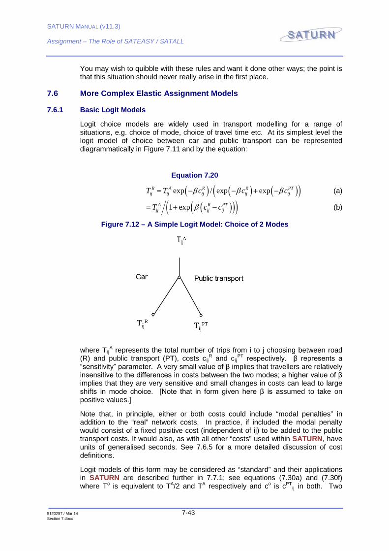
SATURN MANUAL (V11.3)
Assignment – The Role of SATEASY / SATALL
5120257 / Mar 14 7-43 Section 7.docx
You may wish to quibble with these rules and want it done other ways; the point is that this situation should never really arise in the first place.
7.6 More Complex Elastic Assignment Models
7.6.1 Basic Logit Models
Logit choice models are widely used in transport modelling for a range of situations, e.g. choice of mode, choice of travel time etc. At its simplest level the logit model of choice between car and public transport can be represented diagrammatically in Figure 7.11 and by the equation:
Equation 7.20
( ) ( ) ( )( )exp / exp expR A R R PTij ij ij ij ijT T c c cβ β β= − − + − (a)
( )( )( )1 expA R PTij ij ijT c cβ= + − (b)
Figure 7.12 – A Simple Logit Model: Choice of 2 Modes
where TijA represents the total number of trips from i to j choosing between road
(R) and public transport (PT), costs cijR and cij
PT respectively. β represents a “sensitivity” parameter. A very small value of β implies that travellers are relatively insensitive to the differences in costs between the two modes; a higher value of β implies that they are very sensitive and small changes in costs can lead to large shifts in mode choice. [Note that in form given here β is assumed to take on positive values.]
Note that, in principle, either or both costs could include “modal penalties” in addition to the “real” network costs. In practice, if included the modal penalty would consist of a fixed positive cost (independent of ij) to be added to the public transport costs. It would also, as with all other “costs” used within SATURN, have units of generalised seconds. See 7.6.5 for a more detailed discussion of cost definitions.
Logit models of this form may be considered as “standard” and their applications in SATURN are described further in 7.7.1; see equations (7.30a) and (7.30f) where To is equivalent to TA/2 and TA respectively and co is cPT
ij in both. Two
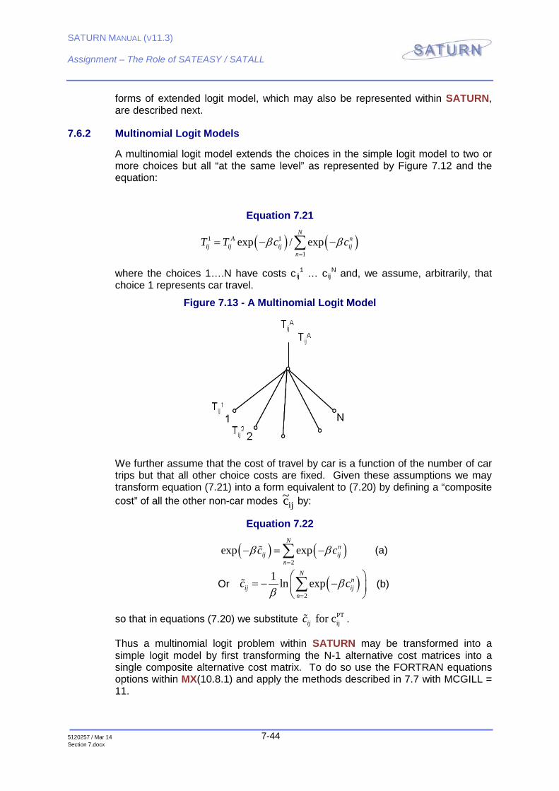
SATURN MANUAL (V11.3)
Assignment – The Role of SATEASY / SATALL
5120257 / Mar 14 7-44 Section 7.docx
forms of extended logit model, which may also be represented within SATURN, are described next.
7.6.2 Multinomial Logit Models
A multinomial logit model extends the choices in the simple logit model to two or more choices but all “at the same level” as represented by Figure 7.12 and the equation:
Equation 7.21
( ) ( )1 1
1exp / exp
NA n
ij ij ij ijn
T T c cβ β=
= − −∑
where the choices 1….N have costs cij1 … cij
N and, we assume, arbitrarily, that choice 1 represents car travel.
Figure 7.13 - A Multinomial Logit Model
We further assume that the cost of travel by car is a function of the number of car trips but that all other choice costs are fixed. Given these assumptions we may transform equation (7.21) into a form equivalent to (7.20) by defining a “composite cost” of all the other non-car modes ijc~ by:
Equation 7.22
( ) ( )2
exp expN
nij ij
nc cβ β
=
− = −∑ (a)
Or ( )2
1 ln expN
nij ij
nc cβ
β =
= − − ∑ (b)
so that in equations (7.20) we substitute PTij for cijc .
Thus a multinomial logit problem within SATURN may be transformed into a simple logit model by first transforming the N-1 alternative cost matrices into a single composite alternative cost matrix. To do so use the FORTRAN equations options within MX(10.8.1) and apply the methods described in 7.7 with MCGILL = 11.
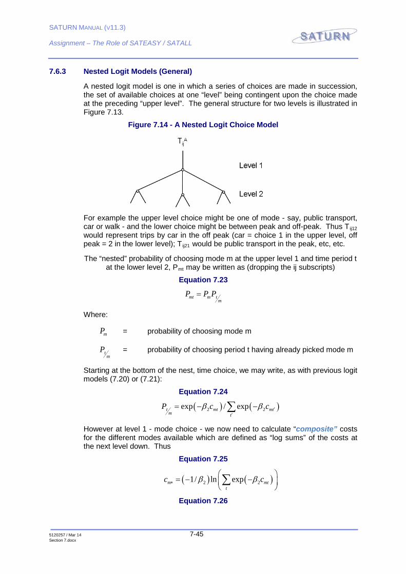
SATURN MANUAL (V11.3)
Assignment – The Role of SATEASY / SATALL
5120257 / Mar 14 7-45 Section 7.docx
7.6.3 Nested Logit Models (General)
A nested logit model is one in which a series of choices are made in succession, the set of available choices at one “level” being contingent upon the choice made at the preceding “upper level”. The general structure for two levels is illustrated in Figure 7.13.
Figure 7.14 - A Nested Logit Choice Model
For example the upper level choice might be one of mode - say, public transport, car or walk - and the lower choice might be between peak and off-peak. Thus Tij12 would represent trips by car in the off peak (car = choice 1 in the upper level, off peak = 2 in the lower level); Tij21 would be public transport in the peak, etc, etc.
The “nested” probability of choosing mode m at the upper level 1 and time period t at the lower level 2, Pmt may be written as (dropping the ij subscripts)
Equation 7.23
mt m tm
P P P=
Where:
mP = probability of choosing mode m
tm
P = probability of choosing period t having already picked mode m
Starting at the bottom of the nest, time choice, we may write, as with previous logit models (7.20) or (7.21):
Equation 7.24
( ) ( )2 2exp / expt mt mtm t
P c cβ β ′′
= − −∑
However at level 1 - mode choice - we now need to calculate “composite” costs for the different modes available which are defined as “log sums” of the costs at the next level down. Thus
Equation 7.25
( ) ( )2 21/ ln expm mtt
c cβ β∗ = − − ∑
Equation 7.26
SATURN MANUAL (V11.3)
Assignment – The Role of SATEASY / SATALL
5120257 / Mar 14 7-46 Section 7.docx
( ) ( )1 1exp / expm m mm
P c cβ β ′∗ ∗′
= − −∑
Note that we use different β values at the two different levels, β 1 β 2, associated with mode and time respectively. For various theoretical reasons logic dictates that β 1 must be less than β2, otherwise the “order” of the nest should be reversed.
Thus starting with the “real” o-d travel costs ctm calculated by mode and time period, which we use directly at the lowest level, we proceed in stages to higher levels where the costs used in the choice processes are composites of the costs further down. If we had a model with three levels of choices, e.g. if car travel in each time period were further subdivided into car driver/car passenger, then the same principles of calculating the composite costs at each level from the (composite) costs at the next level down would still apply.
At the level of “real” network costs these may be either “fixed” or “flow dependent”. For example costs of travel by public transport modes are generally assumed to be independent of the number of passengers per service as well as independent of the levels of congestion on the road. On the other hand travel costs by road are generally assumed to be dependent on the number of vehicles on the road - and hence on the choice process. Models of any level of complexity and interactivity may of course be constructed and algorithms for their solution constructed from the basic SATURN building blocks in the same way that a multinomial logit model (7.6.2) can be transformed into a simple logit model. For the moment we will concentrate on one very basic form of nested logit model.
7.6.4 The Basic Nested Logit Model
Consider therefore a model of two levels, which we shall call “mode” and “time period” but clearly could be anything you wish, with two choices within each level - car/public transport and peak/off-peak. Further assume that we are specifically concerned with a model of cars in the peak and that the costs of the other three choices are fixed. This immediately simplifies the model in that the composite cost for mode choice public transport is also fixed as it is the log sum of fixed public transport costs in the peak and off peak. Denote car choice by 1, public transport by 2 and peak/off peak by 1/2.
The choice model is as represented in Figure 7.14 with, and in what follows, the ij subscripts dropped.
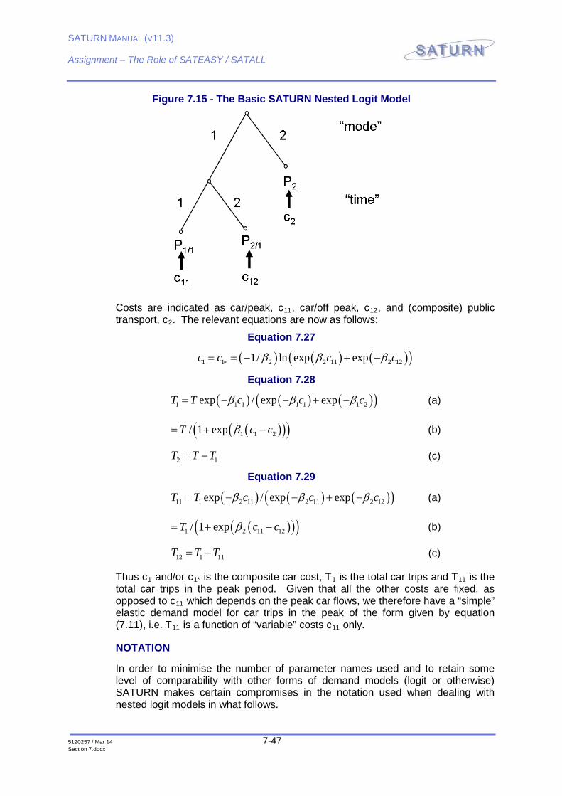
SATURN MANUAL (V11.3)
Assignment – The Role of SATEASY / SATALL
5120257 / Mar 14 7-47 Section 7.docx
Figure 7.15 - The Basic SATURN Nested Logit Model
Costs are indicated as car/peak, c11, car/off peak, c12, and (composite) public transport, c2. The relevant equations are now as follows:
Equation 7.27
( ) ( ) ( )( )1 1 2 2 11 2 121/ ln exp expc c c cβ β β∗= = − + −
Equation 7.28
( ) ( ) ( )( )1 1 1 1 1 1 2exp / exp expT T c c cβ β β= − − + − (a)
( )( )( )1 1 2/ 1 expT c cβ= + − (b)
2 1T T T= − (c)
Equation 7.29
( ) ( ) ( )( )11 1 2 11 2 11 2 12exp / exp expT T c c cβ β β= − − + − (a)
( )( )( )1 2 11 12/ 1 expT c cβ= + − (b)
12 1 11T T T= − (c)
Thus c1 and/or c1* is the composite car cost, T1 is the total car trips and T11 is the total car trips in the peak period. Given that all the other costs are fixed, as opposed to c11 which depends on the peak car flows, we therefore have a “simple” elastic demand model for car trips in the peak of the form given by equation (7.11), i.e. T11 is a function of “variable” costs c11 only.
NOTATION
In order to minimise the number of parameter names used and to retain some level of comparability with other forms of demand models (logit or otherwise) SATURN makes certain compromises in the notation used when dealing with nested logit models in what follows.
SATURN MANUAL (V11.3)
Assignment – The Role of SATEASY / SATALL
5120257 / Mar 14 7-48 Section 7.docx
Thus at the lower level we introduce a parameter BETA_2 to represent β2 and a cost matrix “name” CKLFIL (/FILCKL) to represent c12, the alternative costs at the second level. No problems there. We do however use c2 instead of c12 to denote that cost matrix in the equations from now on.
At the upper level we use the name BETA and the symbol β instead of β1 and denote the alternative cost matrix at this level by “name” CIJFIL (/FILCIJ) and symbol co. This is in line with the other functions used which only require one sensitivity parameter β and one alternative cost matrix. Apologies for any confusion!
7.6.5 Generalised Cost Definitions: Logit vrs. Assignment
By definition the cost cijR that is used in the logit models (or, indeed, any other
form of demand model) is the equilibrium O-D cost that is calculated within the traffic assignment and is therefore based on the definition of cost, as used by the assignment, i.e., as set by PPM and PPK to weight time and distance. However, it may happen that the time/distance weights as calibrated by the demand model may differ or that other components of road costs may need to be included. On the one hand this may indicate basic inconsistencies in the model, i.e., that drivers consider the definition of road costs along one route when they are deciding whether to drive or take the bus but when they get behind the wheel they make quite different route-choice decisions. On the other there may be rational explanations.
For example, a logit-based mode choice analysis might indicate that the utility of car travel increases with increasing distance. In terms of costs, this would imply that costs decrease with distance, hence that PPK should take a negative value and that drivers would prefer to use maximum distance routes (not very sensible in terms of assignment!). However this may also indicate that the disadvantages of public transport travel are positively correlated with distance in ways that cannot be explained by other properties of the public transport service, e.g., in-vehicle time, fares, etc. In this case the positive utility of distance for car travel is actually due to a negative utility for public transport and should therefore not be used as a component of route choice.
The solution in this situation may therefore be to treat the distance component as fixed within the demand model – which, in the above case, would mean including a positive distance cost component within the public transport cost matrix – and to carry out the assignment using pure time (i.e., PPM = 1, PPK = 0). Alternatively, if it is desired to do the assignment with weighted time and distance but the “weights” are different in the logit model, then the situation would be more complex in that the public transport distance component would have to be “corrected” to allow for the fact that the car costs returned from the assignment would also include a distance component. I leave it to you people to work out the equations!
Users who are confused at this point should take expert advice: if you don’t know what you’re doing, don’t do it!
It also needs to be stressed that the road costs are always in units of generalised seconds (or “real” seconds in the case of time-only assignment) and that therefore
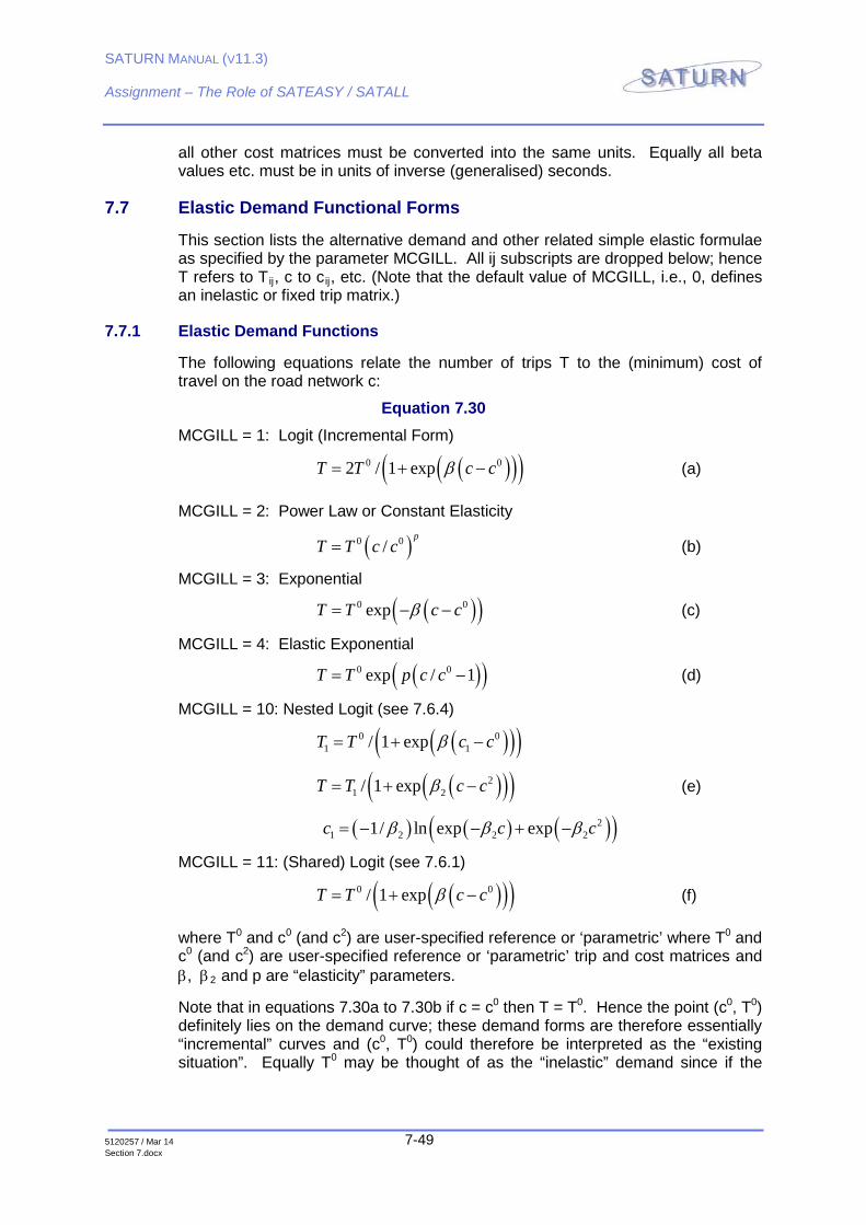
SATURN MANUAL (V11.3)
Assignment – The Role of SATEASY / SATALL
5120257 / Mar 14 7-49 Section 7.docx
all other cost matrices must be converted into the same units. Equally all beta values etc. must be in units of inverse (generalised) seconds.
7.7 Elastic Demand Functional Forms
This section lists the alternative demand and other related simple elastic formulae as specified by the parameter MCGILL. All ij subscripts are dropped below; hence T refers to Tij, c to cij, etc. (Note that the default value of MCGILL, i.e., 0, defines an inelastic or fixed trip matrix.)
7.7.1 Elastic Demand Functions
The following equations relate the number of trips T to the (minimum) cost of travel on the road network c:
Equation 7.30 MCGILL = 1: Logit (Incremental Form)
( )( )( )0 02 / 1 expT T c cβ= + − (a)
MCGILL = 2: Power Law or Constant Elasticity
( )0 0/p
T T c c= (b)
MCGILL = 3: Exponential
( )( )0 0expT T c cβ= − − (c)
MCGILL = 4: Elastic Exponential
( )( )0 0exp / 1T T p c c= − (d)
MCGILL = 10: Nested Logit (see 7.6.4)
( )( )( )0 01 1/ 1 expT T c cβ= + −
( )( )( )21 2/ 1 expT T c cβ= + − (e)
( ) ( ) ( )( )21 2 2 21/ ln exp expc c cβ β β= − − + −
MCGILL = 11: (Shared) Logit (see 7.6.1)
( )( )( )0 0/ 1 expT T c cβ= + − (f)
where T0 and c0 (and c2) are user-specified reference or ‘parametric’ where T0 and c0 (and c2) are user-specified reference or ‘parametric’ trip and cost matrices and β, β2 and p are “elasticity” parameters.
Note that in equations 7.30a to 7.30b if c = c0 then T = T0. Hence the point (c0, T0) definitely lies on the demand curve; these demand forms are therefore essentially “incremental” curves and (c0, T0) could therefore be interpreted as the “existing situation”. Equally T0 may be thought of as the “inelastic” demand since if the

SATURN MANUAL (V11.3)
Assignment – The Role of SATEASY / SATALL
5120257 / Mar 14 7-50 Section 7.docx
costs do not change or if T is independent of c then again T = T0. See 7.8 for further advice as to how to define T0 and c0.
By contrast equations 5 and 6 are “absolute” or “share” demand form equations in which T0 represents a total number of trips, from which a given “share” winds up on the road network. Thus, typically, To as used for share models will be larger than that used by the incremental - e.g. twice as big if the “average” share is 0.5. See 7.5.1.
Note therefore that MCGILL = 1 and MCGILL = 11 both effectively represent exactly the same logit demand model but 1 is expressed in an incremental form and 11 as a share model. In the latter case the input trip matrix T0 would be twice as big.
N.B. The above equations assume that ‘normally’ p will be a negative number and β positive. If the input values have the ‘wrong’ sign, e.g., a positive POWER, then the ‘correct’ sign is automatically used.
See sections 7.12.2 and 7.12.3 for the definitions of the Namelist “names” used to set β, c0 etc within SATURN.
Box-Cox Transformations
An alternative form of simple elastic demand model using what is known as a Box-Cox transformation has been coded into elastic assignment with MCGILL = 5 but its use is highly experimental. Most of the work was carried out by an MSc student Pete Kidd in the 1990’s for his dissertation (indeed an excellent dissertation!) and then incorporated by DVV into the code proper. So blame me for any mistakes!
What follows is probably a highly unreliable description of what Box-Cox does based on faulty memory, Wikipedia and an interpretation of the code.
Basically a Box-Cox transformation is a continuous transformation of a variable x between, at one extreme, the linear function x and, at the other, log(x). More precisely we transform c into c’ via:
C’ = (c** λ – 1) / λ c**( λ-1)
Where λ varies between 0 and 1.0 and in SATURN is defined by the namelist parameter BETA2
What we do in elastic assignment is to substitute a Box-Cox transformation for the OD costs c and c0 in the logit demand equation 7.30a. If BETA2 = 1 c and c0 remains as is the model remains a pure logit model but if BETA2 = 0 c and c0 are transformed into log(c) and log (c0) and mathematically equation 7.30a becomes:
T = 2 T0 / (1 + c**β / c0**β)
= 2 T0 / (1 + (c/c0)** β)
In other words T() is now a function of the relative change in costs rather than the absolute change in costs as per the logit model and therefore much nearer (but not identical) to the power law or constant elasticity model, equation 7.30b.
Therefore what Box-Cox enables one to do is to move continuously between a model based on absolute cost changes to relative cost changes. Which, to my
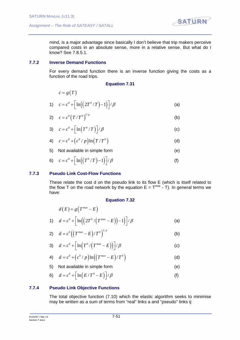
SATURN MANUAL (V11.3)
Assignment – The Role of SATEASY / SATALL
5120257 / Mar 14 7-51 Section 7.docx
mind, is a major advantage since basically I don’t believe that trip makers perceive compared costs in an absolute sense, more in a relative sense. But what do I know? See 7.8.5.1.
7.7.2 Inverse Demand Functions
For every demand function there is an inverse function giving the costs as a function of the road trips.
Equation 7.31
( )c g T=
1) ( )( )0 0ln 2 / 1 /c c T T β = + − (a)
2) ( )1/0 0/p
c c T T= (b)
3) ( )0 0ln / /c c T T β = + (c)
4) ( ) ( )0 0 0/ ln /c c c p T T= + (d)
5) Not available in simple form (e)
6) ( )( )0 0ln / 1 /c c T T β = + − (f)
7.7.3 Pseudo Link Cost-Flow Functions
These relate the cost d on the pseudo link to its flow E (which is itself related to the flow T on the road network by the equation E = Tmax - T). In general terms we have:
Equation 7.32
( ) ( )maxd E g T E= −
1) ( )( )( )0 0 maxln 2 / 1 /d c T T E β = + − −
(a)
2) ( )( )1/0 max 0/p
d c T E T= − (b)
3) ( )( )0 0 maxln / /d c T T E β = + − (c)
4) ( ) ( )( )0 0 max 0/ ln /d c c p T E T= + − (d)
5) Not available in simple form (e)
6) ( )0 0ln / /d c E T E β = + − (f)
7.7.4 Pseudo Link Objective Functions
The total objective function (7.10) which the elastic algorithm seeks to minimise may be written as a sum of terms from “real” links a and “pseudo” links ij:
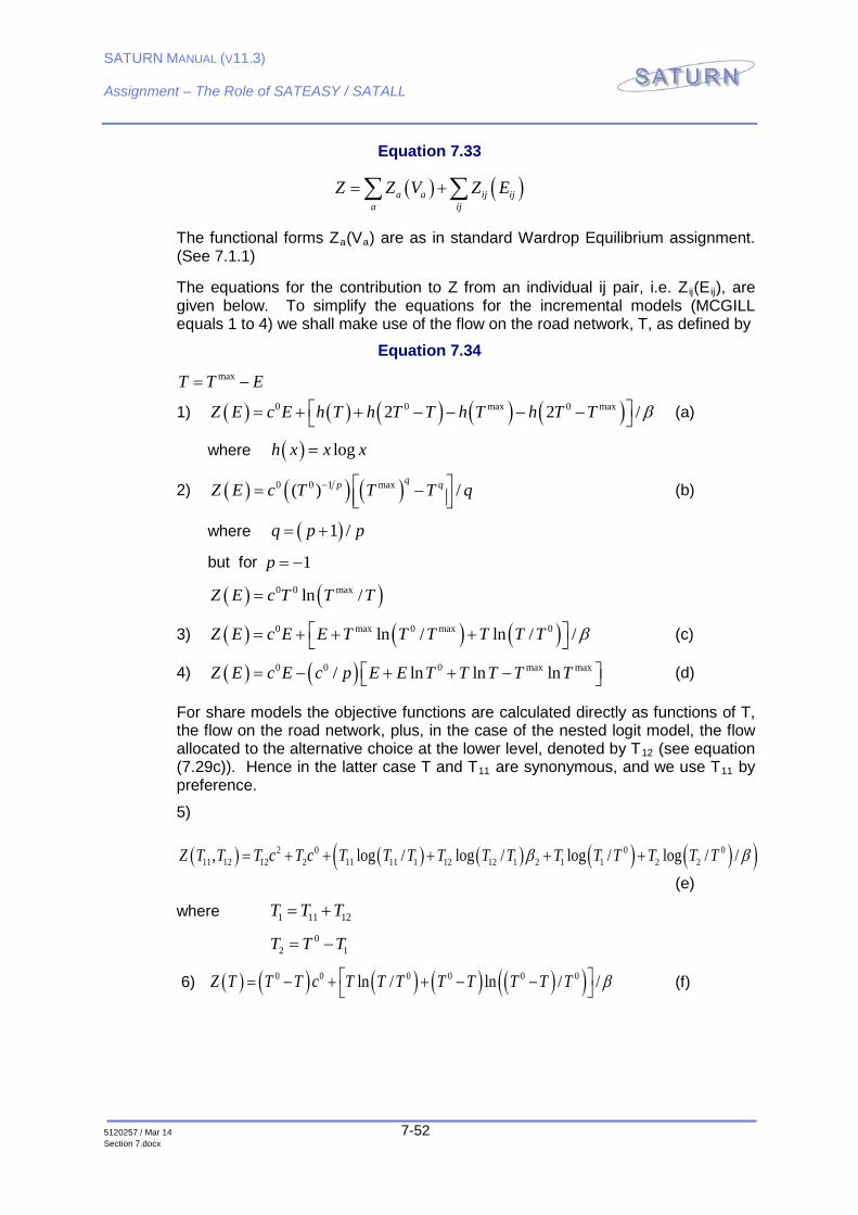
SATURN MANUAL (V11.3)
Assignment – The Role of SATEASY / SATALL
5120257 / Mar 14 7-52 Section 7.docx
Equation 7.33
( ) ( )a a ij ija ij
Z Z V Z E= +∑ ∑
The functional forms Za(Va) are as in standard Wardrop Equilibrium assignment. (See 7.1.1)
The equations for the contribution to Z from an individual ij pair, i.e. Zij(Eij), are given below. To simplify the equations for the incremental models (MCGILL equals 1 to 4) we shall make use of the flow on the road network, T, as defined by
Equation 7.34 maxT T E= −
1) ( ) ( ) ( ) ( ) ( )0 0 max 0 max2 2 /Z E c E h T h T T h T h T T β = + + − − − − (a)
where ( ) logh x x x=
2) ( ) ( ) ( )0 0 1 max( ) /qp qZ E c T T T q− = −
(b)
where ( )1 /q p p= +
but for 1p = −
( ) ( )0 0 maxln /Z E c T T T=
3) ( ) ( ) ( )0 max 0 max 0ln / ln / /Z E c E E T T T T T T β = + + + (c)
4) ( ) ( )0 0 0 max max/ ln ln lnZ E c E c p E E T T T T T = − + + − (d)
For share models the objective functions are calculated directly as functions of T, the flow on the road network, plus, in the case of the nested logit model, the flow allocated to the alternative choice at the lower level, denoted by T12 (see equation (7.29c)). Hence in the latter case T and T11 are synonymous, and we use T11 by preference.
5) ( ) ( ) ( ) ( ) ( )( )2 0 0 0
11 12 12 2 11 11 1 12 12 1 2 1 1 2 2, log / log / log / log / /Z T T T c T c T T T T T T T T T T T Tβ β= + + + + +
(e)
where 1 11 12T T T= +
02 1T T T= −
6) ( ) ( ) ( ) ( ) ( )( )0 0 0 0 0 0ln / ln / /Z T T T c T T T T T T T T β = − + + − − (f)

SATURN MANUAL (V11.3)
Assignment – The Role of SATEASY / SATALL
5120257 / Mar 14 7-53 Section 7.docx
7.7.5 Elasticities
The ‘elasticity’ of trip demand with respect to changes in cost is defined by
Equation 7.35
( ) ( )/ / /e dT T dc c=
where dT represents the change in the number of trips T in response to a change in costs of dc in c. Since T is a decreasing function of c e must be negative although it is not uncommon for non-economists to refer to its absolute values (the reason why SATURN allows positive values of POWER and BETA but converts them into negative).
With the simple power law function the elasticity is a constant over all ij pairs and equal to the parameter POWER; with the other functions elasticity is a function of both Tij and cij and the following functions apply:
1) ( )( ) ( )( )( )0 0exp / 1 expe c c c c cβ β β= − − + − (a)
( )0 02 / 2c T T Tβ= − −
2) e p= (b)
3) e cβ= − (c)
4) 0/e pc c= (d)
5) ( )1 11 1 2/e e T T e= + (e)
where e1 and e2 are the elasticities in the upper and lower levels respectively and may be given by equations such as (7.35a) or (7.35f). For the definitions of T11 and T1 see section 7.6.4.
6) ( )( ) ( )( )( )0exp / 1 exp oe c c c c cβ β β= − − + − (f)
( ) 01 /c T Tβ= − −
The alternative versions of equations (7.35a) and (7.35f) which use trips T (or, strictly speaking, proportions of trips choosing car travel) in addition to costs are based on standard results from logit theory and are certainly easier to work with then those based entirely on costs.
7.7.6 Empirical Elasticities
Elasticities may also be calculated empirically. In SATEASY/ SATALL this is done (pre-assignment and - see below - post-assignment) by calculating the total numbers of trips with the cost matrix cij = cij
0 and with cij = 1.01cij0; the difference
in total number of trips provides a measure of dT in equation (7.35). In the case of multiple user classes the empirical elasticities may be disaggregated by user classes (11.11.7). The values are printed within the .lpt/lpa output files.
In the case of the power law or constant elasticity model (MCGILL = 2) the empirical elasticity should correctly equal the input value (POWER), in which case

SATURN MANUAL (V11.3)
Assignment – The Role of SATEASY / SATALL
5120257 / Mar 14 7-54 Section 7.docx
there is very little point in carrying out the calculations. However for other model forms the relationship between, say, BETA values and the elasticity is not direct and the empirical values can be a useful guide (see also the final paragraph in this section).
Note however that for all cases apart from MCGILL = 2 the elasticities are not constant but depend on the point on the demand curves where the calculations are made, i.e., on the road costs and/or number of road trips. Ideally one would probably prefer the elasticities to be calculated using the actual output costs and trips from the elastic assignment. However the first set of values reported by SATALL are those that would apply if the costs of travel by road equal c0 which are not necessarily all that close to the output costs.
In the case of (most) incremental models those costs are probably fairly close to the final costs given the manner in which they would have been defined and the reported elasticities should be good estimates. However for the various forms of logit choice models (MCGILL = 1, 10 or 11) the costs c0 may represent costs, say, by public transport, in which case they may be a long way away from the “true” road costs and any elasticity calculated at those costs need to be taken with a large pinch of salt.
For this reason for MCGILL = 10 or 11 (i.e, shared demand models) the empirical elasticities are also calculated after the assignment has taken place and using the minimum ij road costs in place of c0. These elasticities are therefore more realistic and may differ considerably from those reported pre-assignment. They are also reported within the lpt/lpa files.
It should also be remembered that elasticities vary by od cell (except of course for the constant elasticity form). Elasticities may, in principle, be calculated cell by cell using the equation editor in MX based on the “correct” costs and/or road trips and trip-weighted averages obtained.
In order to detect consistent differences in elasticities by trip length (with logit-based models elasticities increase with cost; see equation 7.35a) the reported empirical elasticities are disaggregated by cost bands expressed in terms of generalised costs in minutes – new in 10.8.20. These are printed within the .LPT files. Note that the differences, especially with logit models, may be significant and users may wish to consider this in their choice of: (1) the form of the demand model and (2) the calibration parameters.
The calculated empirical elasticities are stored within the output .ufs files and may also be accessed within the network parameters printed by SATLOOK. In the case of MCGILL = 10 or 11 the values stored are those calculated post assignment as explained above.
We note again that POWER is very closely associated with elasticity (and exactly equal for MCGILL = 2) and therefore (a) is assigned very similar values of the order of, say, -0.5, and (b) is unitless. By contrast BETA is only a parameter which defines elasticity in part and (a) has units of inverse generalised cost and (b) takes values which bear no direct relationship to the value of the intended elasticities.
If the empirical elasticity is extremely high (in absolute terms), e.g., -10.0, then SATALL may refuse to run on the grounds that: (a) it may fail due to problems with numerical underflow or overflow and (b) it is most unlikely that this is what the

SATURN MANUAL (V11.3)
Assignment – The Role of SATEASY / SATALL
5120257 / Mar 14 7-55 Section 7.docx
user actually wanted to do. The two most common causes of extreme elasticities (either very high or very low) are: (a) users confusing BETA and POWER and therefore setting BETA to an appropriate value of POWER or vice-versa, or (b) defining BETA values in the wrong units (e.g., inverse minutes rather than inverse seconds).
7.8 Defining the Reference Trip and Cost Matrices
The first point to be made is that the choice of a functional form for the demand function and of the files and parameters necessary to specify it is entirely up to the user. Elastic assignment is very much a situation where the user must tell the model/program what to do, not the other way round. The purpose of this section is therefore purely to offer advice to users who (of course!) know what they want to do but (naturally!) may be a little uncertain on the way to go about it.
The second point is that the use of a superscript 0 to define Tij0 and Cij
0 should not be taken as implying that they necessarily represent a “base point”, e.g. a do-minimum scenario in year zero. They are parametric or reference matrices used to define a demand function; in some situations they may be conveniently defined as a base point, in others not. In certain situations they may also depend on the scenario; e.g. a “do something” land use scheme may affect growth factors for certain O’s and D’s and hence influence the definition of Tij
0.
It is also important to remember that cost matrices must be defined as generalised costs with units of seconds. Care must therefore be exercised when importing cost matrices (e.g., public transport cost matrices) from other suites of programs.
Their interpretation also differs in some respects between the incremental model forms (MCGILL = 1 to 4) and the shared forms (MCGILL = 10 or 11); we consider these separately.
7.8.1 Incremental Models
In general terms the elastic demand function represents a situation where, all other things being equal, the number of trips is expected to decline when costs increase although the precise mechanism (change of travel time, change of mode etc.) is not specified. A common property of all the 4 incremental demand functions in these cases is that if the ij costs = c0
ij then the ij flow = T0ij; this
defines one point on the demand curve. This is illustrated in Figure 7.15.
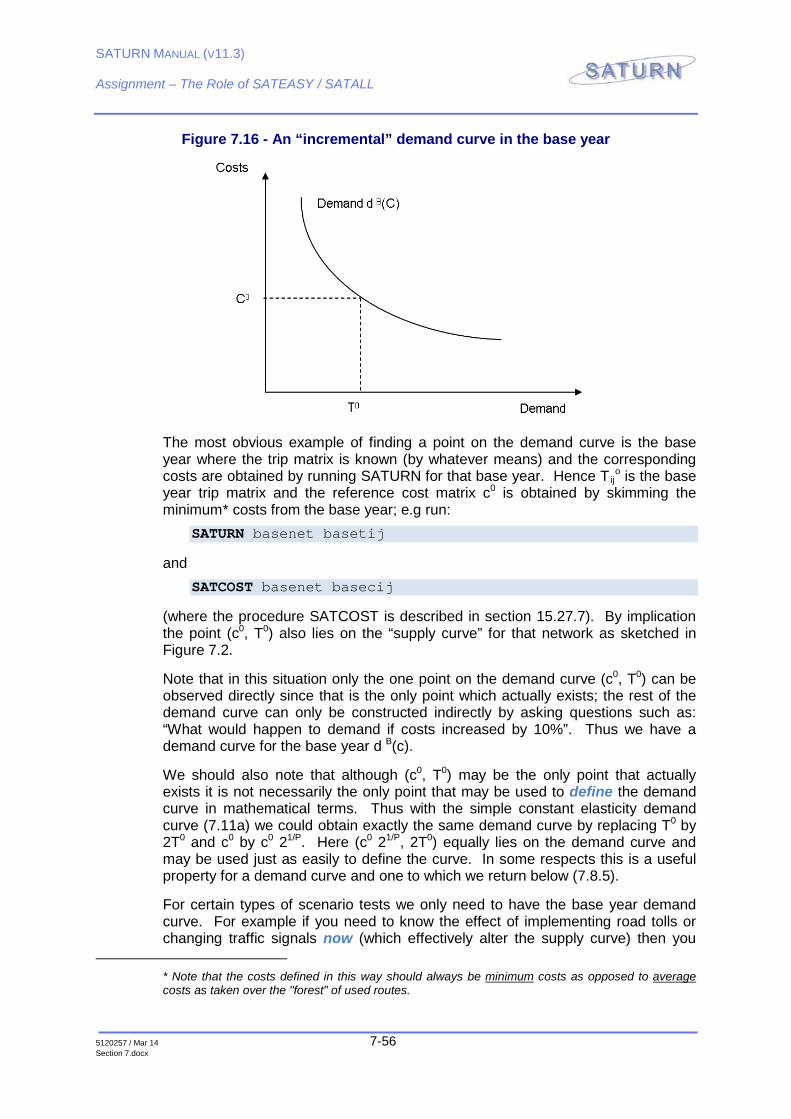
SATURN MANUAL (V11.3)
Assignment – The Role of SATEASY / SATALL
5120257 / Mar 14 7-56 Section 7.docx
Figure 7.16 - An “incremental” demand curve in the base year
The most obvious example of finding a point on the demand curve is the base year where the trip matrix is known (by whatever means) and the corresponding costs are obtained by running SATURN for that base year. Hence Tij
o is the base year trip matrix and the reference cost matrix c0 is obtained by skimming the minimum* costs from the base year; e.g run:
SATURN basenet basetij
and SATCOST basenet basecij
(where the procedure SATCOST is described in section 15.27.7). By implication the point (c0, T0) also lies on the “supply curve” for that network as sketched in Figure 7.2.
Note that in this situation only the one point on the demand curve (c0, T0) can be observed directly since that is the only point which actually exists; the rest of the demand curve can only be constructed indirectly by asking questions such as: “What would happen to demand if costs increased by 10%”. Thus we have a demand curve for the base year d B(c).
We should also note that although (c0, T0) may be the only point that actually exists it is not necessarily the only point that may be used to define the demand curve in mathematical terms. Thus with the simple constant elasticity demand curve (7.11a) we could obtain exactly the same demand curve by replacing T0 by 2T0 and c0 by c0 21/P. Here (c0 21/P, 2T0) equally lies on the demand curve and may be used just as easily to define the curve. In some respects this is a useful property for a demand curve and one to which we return below (7.8.5).
For certain types of scenario tests we only need to have the base year demand curve. For example if you need to know the effect of implementing road tolls or changing traffic signals now (which effectively alter the supply curve) then you
* Note that the costs defined in this way should always be minimum costs as opposed to average costs as taken over the "forest" of used routes.

SATURN MANUAL (V11.3)
Assignment – The Role of SATEASY / SATALL
5120257 / Mar 14 7-57 Section 7.docx
require the new equilibrium point between the new supply curve and the existing demand curve. Thus, Figure 7.16, if we shift the supply curve from S1 to S2 we change the equilibrium point from (T1*, C1*) to (T2*, C2*)
Figure 7.17 - New Supply Curves: A New Equilibrium
In this case (since S2 is above S1 implying higher costs) we have both increased the equilibrium costs (C2* > C1*) and decreased the demand for trips (T2* < T1*). Note that had we modelled the new scenario with fixed trips we would have wound up at the equilibrium (T1*, C2
F) which would imply higher costs than in the “correct” equilibrium state.
FUTURE YEARS
For future years the demand curve must also allow for exogenous growth, e.g through increased housing, employment or car ownership via growth factors which implicitly assume that travel costs do not change. Thus we might predict a uniform 10% growth in the trip matrix by some future year if there is no change in congestion. We may therefore construct a future year demand curve dF(c ) from the base year demand curve dB(c) by simply applying a factor of 1.1 to all demand values on the curve. See Fig. 7.17. Thus the point (c0, 1.1T0) should definitely lie on the new demand curve.

SATURN MANUAL (V11.3)
Assignment – The Role of SATEASY / SATALL
5120257 / Mar 14 7-58 Section 7.docx
Figure 7.18 - Base Year and Future Year Demand Curves (dB and dF) plus Alternative Supply Curves S1 and S2.
However, this is not to say that the point (c0, 1.1T0) is a valid forecast of some future scenario since it does not take into account the extra congestion generated by the extra 10% traffic demand which will alter the costs. It simply says that if the costs remain as they are in the base year then trips will grow by 10%. Elastic assignment introduces the effect of added congestion.
Thus in Figure 7.17 if point A - (c0, T0) - represents the base year equilibrium point E represents the future year scenario - (c0, 1.1T0) - if costs remain fixed. However if the network continues to operate according to supply curve S1 we would wind up at point B in the future year with: (a) higher costs than c0 and (b) fewer trips than 1.1T0. In this case the elasticity effects are suppressing trips.
Equally if we consider alternative network scenarios as represented by supply curve S2 in Figure 7.17 then the future year equilibrium would be represented by point D - in this case fewer trips and increased costs relative to point B.
Note therefore that points E, B and D all lie on the future year demand curve and that all three represent equally valid forecasts of future year traffic levels given certain assumptions about what the costs will be.
To define the future year demand curve using as input a reference cost matrix and a reference trip matrix you are recommended to use the base year cost matrix c0 for the future year as well but the future year reference trip matrix would be the base year matrix factored by 1.1; use MX to do this. (The alternative use of GONZO = 1.10 is feasible but not recommended since if you start to compare future year elastic and inelastic trip matrices it can be very confusing trying to remember whether they include a GONZO factor or not).

SATURN MANUAL (V11.3)
Assignment – The Role of SATEASY / SATALL
5120257 / Mar 14 7-59 Section 7.docx
7.8.2 Base Year Logit Models
Another, more explicit, application of SDM elastic assessment is to model modal split, e.g via a logit equation of the form:
( ) ( ) ( )( )exp / exp expA R R PTij ij ij ij ijT T c c cβ β β= − − + − (a)
( )( )( )/ 1 expA R PTij ij ijT c cβ+ − (b)
where the superscripts R and PT represent road and public transport and TijA
represents the total number of ij trips. See 7.6.1. As noted in 7.5.1 the public transport costs could include a (positive) perceived modal penalty.
Logit models may be represented either in an incremental or shared form - and in some respects the latter formulation, discussed in 7.8.4, is more “natural”. The following considers it primarily in the incremental form (MCGILL = 1).
Comparing equation (7.20b) with the incremental logit equation (7.30a) it can be seen that c0 is equivalent to cPT and Tij
A to 2T0. Hence in this case the reference trip matrix refers to public transport costs and would need to be obtained from a public transport assignment program such as SATCHMO. Equally we would need to define T0
ij = TAij/2.
Note that in this case the necessary reference matrices Tij0 and cij
0 should certainly not be interpreted as a base point for road traffic since they do not correspond to any “real” observed values of road trip matrices or costs - except in the most unlikely case of all road costs being identical to public transport costs and the modal split therefore being 50:50.
However, in the event that we know the base-year road trip matrix and road costs, which we will denote by Tb and cb, and we know the total number of trips TA (e.g. if we know the “share” of road trips) then we can work out the (unknown) public transport cost matrix cPT = c0 by the matrix transformation (e.g., use MX):
Equation 7.36
( ) ( )( )0 1/ ln /b A b bc c T T Tβ= − −
The logit demand curve is sketched in Figure 7.18 where both the base year point (cb, Tb) and the reference point (c0, T0) lie on the curve. Note that to specify the precise form of this demand function a single point on the function (plus a value for β) is not enough, we need extra information to specify TA.
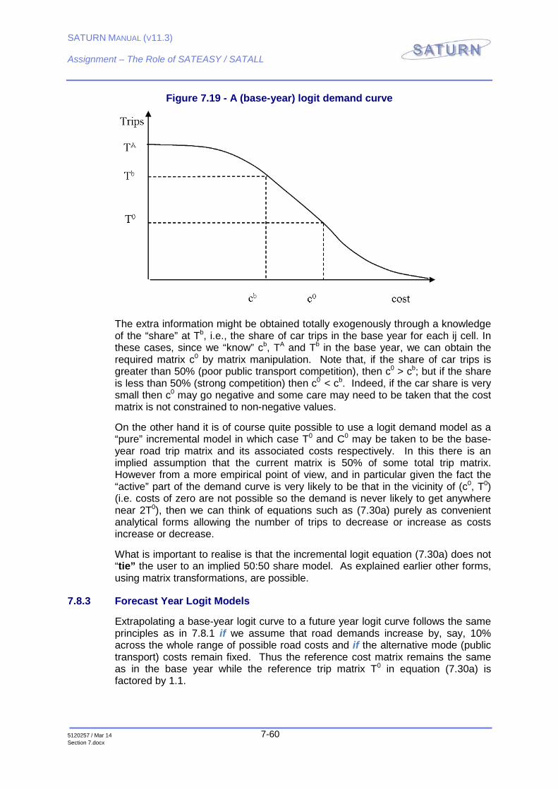
SATURN MANUAL (V11.3)
Assignment – The Role of SATEASY / SATALL
5120257 / Mar 14 7-60 Section 7.docx
Figure 7.19 - A (base-year) logit demand curve
The extra information might be obtained totally exogenously through a knowledge of the “share” at Tb, i.e., the share of car trips in the base year for each ij cell. In these cases, since we “know” cb, TA and Tb in the base year, we can obtain the required matrix c0 by matrix manipulation. Note that, if the share of car trips is greater than 50% (poor public transport competition), then c0 > cb; but if the share is less than 50% (strong competition) then c0 < cb. Indeed, if the car share is very small then c0 may go negative and some care may need to be taken that the cost matrix is not constrained to non-negative values.
On the other hand it is of course quite possible to use a logit demand model as a “pure” incremental model in which case T0 and C0 may be taken to be the base-year road trip matrix and its associated costs respectively. In this there is an implied assumption that the current matrix is 50% of some total trip matrix. However from a more empirical point of view, and in particular given the fact the “active” part of the demand curve is very likely to be that in the vicinity of (c0, T0) (i.e. costs of zero are not possible so the demand is never likely to get anywhere near 2T0), then we can think of equations such as (7.30a) purely as convenient analytical forms allowing the number of trips to decrease or increase as costs increase or decrease.
What is important to realise is that the incremental logit equation (7.30a) does not “tie” the user to an implied 50:50 share model. As explained earlier other forms, using matrix transformations, are possible.
7.8.3 Forecast Year Logit Models
Extrapolating a base-year logit curve to a future year logit curve follows the same principles as in 7.8.1 if we assume that road demands increase by, say, 10% across the whole range of possible road costs and if the alternative mode (public transport) costs remain fixed. Thus the reference cost matrix remains the same as in the base year while the reference trip matrix T0 in equation (7.30a) is factored by 1.1.
SATURN MANUAL (V11.3)
Assignment – The Role of SATEASY / SATALL
5120257 / Mar 14 7-61 Section 7.docx
Note, from a purely technical point of view, that it may be possible to factor a base year trip matrix by setting GONZO = 1.1 (say). However, this is not recommended.
7.8.4 Share Models
With the share models, MCGILL = 10 or 11, the interpretation of the input trip and cost matrices is more constrained since they represent a simple (2-level, 2-choice) nested logit model and a basic logit model respectively.
Hence Tij0 in equations (7.30e) and (7.30f) represents the total number of trips
between i and j with certain (user-defined) choices to be made. Hence it is the equivalent of TA in Figure 7.6, not T0. In the base year this might represent an observed matrix (aggregated over all choices); in an alternative/future year scenario it could represent the base year matrix suitably growthed up either uniformly or by origin or destination to represent specific local schemes.
The interpretation of the alternative or “parametric” cost matrix (or matrices with nested logit) is also more constrained since it/they must represent the cost(s) by well-defined alternative choices. Hence they are not base-year road costs (although, as with equation (7.36) they may be inferred from road costs given sufficient extra information.
Since the alternative costs are not road related their values in future years will need to be determined by the user. Thus if c0 represents costs by public transport it may be necessary to calculate them based on future year levels of service, fares etc.
7.8.5 Choice of Demand Function
The most important single consideration in establishing a demand function is to get the right degree of sensitivity of demand to costs, the best single measure of which is elasticity. At a global level, i.e. in terms of the total number of trips by road, it is possible, by a judicious choice of β and/or p parameters, to make all demand functions “look” very similar as long as the costs do not diverge too much from their “base” levels. However if we look at the different functions at a more disaggregate level, e.g. origin or o-d level, then marked differences do appear between the different functions as discussed below.
7.8.5.1 Absolute vrs Relative
The logit and exponential demand functions - (7.30a) and (7.30c) - are functions of absolute differences in costs while the power law and elastic exponential forms - (7.30b) and (7.30d) - depend on the relative differences or cost ratios. Thus in the latter case there is no difference between costs which change from 10 to 11 minutes or from 100 to 110 minutes. With an absolute function 100 to 110 minutes would have (effectively) 10 times the impact as 10 to 11.
This implies that absolute models will tend to have a greater effect on long distance trips than short simply because long distance trips include more links which can contribute to cost differences. However this may depend on the type of policy being tested. For example if the cost changes are due to tolls on a single link or a cordon which is crossed only once then all trips will experience the same
SATURN MANUAL (V11.3)
Assignment – The Role of SATEASY / SATALL
5120257 / Mar 14 7-62 Section 7.docx
increase in cost (or zero), in which case, relatively speaking, short distance trips will be greater affected with a relative model.
This is not to say that absolute models are better than relative or vice-versa; beauty is in the eye of the beholder and you need to make up your own mind. But, at the very least, be aware of possible differences.
7.8.5.2 Limiting Values
The functions differ further in how they behave in the limits of very high and very low costs. Thus at zero cost the power law demand goes to infinity whereas all other models approach finite values. This may seem a fairly “academic” distinction in that zero-cost trips do not exist in real life, at any rate between zones by car. However they may well crop up in models.
Thus in network models it is certainly not unusual for two zones to be attached to the same node, in which case their o-d costs are likely to be “modelled” as zero. Alternatively they may be connected at opposite sides of a single simulated turn with a delay of very near zero, in which cases any changes at that node which lead to finite delays (e.g. converting a priority junction to signals) may lead to very large and presumably very unrealistic changes in the demand.
This should not be seen as a reason why not to use power law functions; however it is a factor that the user needs to be aware of and to guard against.
Equally at very high costs the exponential functions will tend to go to zero more rapidly than the power functions although, since the absolute numbers of trips will be near zero in either case, the differences will be less pronounced.
7.8.5.3 Base Independence
All the elastic demand functions in 7.7.1 may be written in the general form:
( )0 0,T T f c c=
where, by definition, f(c0, c0) = 1. The point (T0, c0) may be thought of as a “base” or “pivot point” through which the demand function must pass. It turns out that some, but not all, of the functions in 7.7.1 have the additional property of being “base independent” in that any point on the demand curve may be chosen as the base point and the identical function is produced.
For “base dependent” functions (T0, c0) has a more precise definition so that, in practical terms more care is needed on the part of the user to specify them.
To illustrate, consider the constant elasticity form (7.30b):
( )0 0/P
T T c c=
( )( )0 0/P PT T c c=
0 PT X c=
In this case we need only one value X0 to specify the form of the demand function (assuming the elasticity p to be specified separately), not two separate values of

SATURN MANUAL (V11.3)
Assignment – The Role of SATEASY / SATALL
5120257 / Mar 14 7-63 Section 7.docx
T0 and c0. It also follows that X0 may be obtained from any other point on the demand curve, say (T1, c1) since
0 11/ PX T c=
Similarly, equation (7.30c), may be written:
( )( )0 0expT T c cβ= − −
( ) ( )0 0exp expT T c cβ β= −
( )0 expT X cβ= −
such that any point on the curve is sufficient to define X0.
However the logit equation (7.30a) cannot be rewritten as above, i.e. with the dependence on c separated from the dependence on T0 and c0. Hence it is base dependent. Similarly the elastic exponential (7.30d) and the nested logit (7.30e) are base dependent.
If we refer to (T0, c0) as the base scenario A for some future year we may, with base independent functions, use the T0 and c0 matrices as the base to carry out an elastic assignment for scenario B with, e.g. a changed network. If we then wish to consider another scenario, C, then we may use either the matrices from scenario A or from scenario B as our starting point; both will give the same results*. This would not be true with a base dependent function.
In practical terms base independent functions give the user a bit more flexibility. If you accidentally delete the matrices from scenario A above but still have those from scenario B then you are OK. On the other hand if you are the sort of person that goes around deleting important files then you are probably the sort of person who could accidentally use a trip matrix from scenario B and a cost matrix from scenario C as the base for scenario D and wind up with totally the wrong result whether your basic function is base independent or not.
On balance there is no substitute for being careful and base dependence/independence should not be seen as favouring one functional form in preference to another.
7.8.6 The Definition of “Cost” within Demand and Supply Models
In our general discussion of the equilibrium between supply (i.e., assignment) and demand models in Section 7.4.1 it was implicitly assumed that the “cost” as defined within the assignment model is identical to the cost as defined within the demand model. (Or, strictly speaking, we assume that the route-dependent components of the cost are the same in both models.) However it is not uncommon for combined VDM models to be formulated in which this rule is not adhered to.
* Strictly speaking both will converge towards the same results but since they are likely to start from different initial conditions they may yield slightly different results since they will be converging along different paths.
SATURN MANUAL (V11.3)
Assignment – The Role of SATEASY / SATALL
5120257 / Mar 14 7-64 Section 7.docx
For example, the cost as used in the demand model may include components such as vehicle operating costs which are based on an average speed of travel between O and D which, in turn, depends upon the route(s) used but which, cannot be calculated as a straightforward sum of individual link components along the route(s); i.e., we cannot define an additive operating cost per link. Equally the demand model may use the same components of cost as the assignment model, i.e., time and distance, but use different weights. Or, frequently, the demand model may use a different level of disaggregation into user classes (with, generally, more user classes in the demand model than in the assignment model).
In all such cases there is a strong possibility that the combined supply-demand model will not converge to a unique equilibrium solution (either it will become stuck in infinite loops or there may be multiple equilibria, one of which will be arbitrarily reached). The basic problem is that the two models are “pulling in opposite directions”.
Note that the problem does not occur if the demand model includes cost components which do not feature in the route choice models as long as those cost components are totally independent of the routes chosen. For example, modal split models frequently add a notional penalty to the O-D costs by public transport but these costs have no affect on the choice of an O-D route by either road or public transport. Similarly, if area licensing is being modelled such that a trip with both origin and destination within the charge area automatically pays a toll but that toll is fixed independent of the route chosen, it is not necessary to include that toll within the assignment model; it can be subsequently added to the O-D cost matrix for those cells as a pure matrix operation. By contrast including, as above, a vehicle operating cost based on speed is clearly route-dependent.
A more practical consideration is that, in order to calculate an average O-D speed or to set up cost matrices based on different time/distance weights, etc. etc., it becomes necessary to build skimmed (“forest”) matrices of O-D time and distance from the assignment model. However this leads to a number of practical difficulties (see 15.27.6):
(a) Considerable CPU overheads involved in skimming time, distance, etc. matrices compared to calculating a minimum cost matrix (in addition to the extra CPU overheads involved in carrying out the extra SAVEIT assignment in the first place);
(b) Problems of differences between the SAVEIT and “master” assignments (15.23.2) and
(c) Problems associated with the non-uniqueness of route flows and therefore the non-uniqueness of skimmed time etc. matrices (7.1.6, 15.23.8 and 15.27.6).
By contrast a demand model which is based on minimum cost matrices from the assignment requires a single tree build per origin to build a cost matrix, is based on the final set of (unique) equilibrium link costs and is, therefore, also unique.
While clearly we would not wish to prevent users from setting up demand models which involve different definitions of O-D costs if they wish to do so, it is not, however, a practice that we (DVV) would particularly recommend. From a
SATURN MANUAL (V11.3)
Assignment – The Role of SATEASY / SATALL
5120257 / Mar 14 7-65 Section 7.docx
behavioral point of view, it does not make much sense to me to assume that drivers react in one way to road costs when evaluating route choice but in a different way when evaluating, say, destination choice. Caveat emptor!
Our strong recommendation is, therefore, to use the minimum cost O-D matrices from the road assignment as the costs input to the demand model unless there are compelling reasons for doing otherwise.
In terms of the various standard batch files to calculate cost matrices as described in Section 15.27.7 our recommendation is to use SATCOST in preference to SATC_AV – option 14 in preference to option 9 in SATLOOK.
Finally we note that very similar considerations apply to linkages between SATURN and economic evaluation models such as TUBA (15.41.1); i.e., life becomes considerably simpler if the evaluation framework only requires a minimum cost O-D matrix as opposed to a breakdown by time, distance, etc. etc.
7.8.7 Conclusions
To reiterate the first point made in this section - the choice and definition of the demand function is entirely up to the user. All this section contains is advice, albeit very sound advice!
Thus, at its simplest, elastic assignment may involve nothing more than uniformly factoring up an existing trip matrix by 10 or 20% as the “new” base point and using a present-day cost matrix. On the other hand the demand process may be part of a much more involved multi-stage process. The choice is yours. If you understand what your demand model represents and how to specify it then you should have no problems; if you are not sure what you are doing then our advice would be to keep it as simple as possible.
Finally, whether you are an expert or a beginner, it is a very good idea to check at least once that the outputs from an elastic assignment model are indeed consistent with your demand model. Thus having run an elastic model and produced an output road trip matrix Tij use SATCOST (15.27.7) to calculate the new cost matrix cij. You should then be able to use the FORTRAN equation editor in MX to independently calculate Tij from the input matrices Tij
0, cij0, and cij (use
the equations in 7.7.1). If the two versions of Tij are "near" one another, e.g. +1% per o-d element then your method is probably sound; if not, check your process carefully. Do not expect 100% agreement which will only occur for perfect convergence.
7.9 Multiple User Class Elastic Assignment
Multiple User Class Elastic Assignment combines the concepts of multiple user classes (see 7.3) and of cost-sensitive trip matrices (see 7.5.1) so that each of the NOMADS user classes has a different demand function; hence:
Equation 7.37
( )ijm ijm ijmT f c=
where the additional subscript m refers to a different user class.

SATURN MANUAL (V11.3)
Assignment – The Role of SATEASY / SATALL
5120257 / Mar 14 7-66 Section 7.docx
Alternatively the demand functions may be the same but the definition of generalised cost (6.11) may differ between user classes, e.g., via tolls.
Running MUC elastic assignment requires that the extra trip and cost matrices, both input and output, i.e., cij
0, Tij' and Tij are “stacked” matrices with a distinct level for each user class. Strictly speaking the “reference” input trip matrix Tij
0 need not be stacked so that two different classes may “share” the same trip matrix but with different factors (see the definition of a "matrix level" in 6.11) but to avoid confusion and to facilitate the comparison of input and output matrices it is probably best to “stack” To
ij; see the warning at the end of 7.3.1.2.
The same condition applies to the frozen trip matrix (FILICE) if ICING = T and, indeed, any other input matrices; i.e., that it is “stacked” with a distinct level for each user class.
Class specific demand functions may be specified by defining individual values of MCGILL (which sets the functional form) and BETA/POWER etc (which set the elasticities). See 7.12.2. Thus it is possible to model two different classes of drivers, one of which has a very high elasticity (i.e., is very sensitive to changes in travel costs) and one of which has a low elasticity (i.e., tends to travel independent of the costs).
Note the parameters MCGILL, BETA and POWER are “subscripted” variables here; i.e., rather than setting MCGILL = 1 you will need to set MCGILL(1) = 1 for user class 1. However it is also possible to set a “universal” value of MCGILL for all user classes by including a definition of the form MCGILL = 1 but no definitions of the form MCGILL(1) = 1. Similar considerations apply to BETA and POWER.
It is possible - and not infrequent - to carry out a “mixed” elastic/inelastic MUC assignment in which certain classes are assigned as fixed trip matrices while others are elastic. To do so simply set the user-class specific value of MCGILL to zero; e.g. set MCGILL(1) = 2 and MCGILL(2) = 0 to have user class 1 elastic and class 2 fixed.
It is equally feasible to use either incremental or shared demand functions (see 7.5.1) but it is not possible to “mix” them between classes. Thus MCGILL(1) = 2 and MCGILL(2) = 11 is not a permitted combination.
For further information on multiple user class elastic assignment please refer to Appendix C.
7.10 Combined Distribution and Assignment Models
7.10.1 General Principles
Two forms of distribution models are available within SATURN, both of which are “origin-constrained” and both of which are based on the logit formulation:
1. Incremental:
Equation 7.38
( )( )0 0expij i ij ij ijT AT c cβ= − −
2. Absolute or shared:
SATURN MANUAL (V11.3)
Assignment – The Role of SATEASY / SATALL
5120257 / Mar 14 7-67 Section 7.docx
Equation 7.39
( )expij i ijT A cβ= −
where in both cases the balancing factors Ai are chosen such that:
Equation 7.40
ij ij
T O=∑
where Oi = the number of trips originating from i as calculated from the origin sums in the “base” matrix Tij
o.
Clearly the incremental model requires two additional input files to define a “base” trip matrix To
ij and a "base" cost matrix coij. Less clearly the absolute model (7.39)
also requires an input trip matrix which is used only to define origin trip ends (although it would not be too complicated to input the trips ends directly if required; apply to DVV!)
In both cases an equivalent optimisation representation of the problem is available such that the combined distribution plus assignment problem may be solved using very similar algorithms to those used to solve “simple” elasticity problems; see 7.5.2.
Note that distribution may be run either “on its own”, i.e., as a model of combined distribution and assignment, or in combination with further demand stages such as modal split. See 7.10.4.
7.10.2 Control Parameters
The choice of distribution model is controlled by the parameter MCUBC (7.12.2) where:
MCUBC = 0 No distribution (default)
MCUBC = 1 Incremental
MCUBC = 2 Absolute
The “sensitivity” parameter β in equations (7.38) and (7.39) is set by parameter BETA_D (7.12.2).
Both MCUBC and BETA_D may be either set via the original network .dat file input to SATNET (see 6.3) or in the control files input to SATEASY or SATALL; see 7.12.2 and 9.15.2 respectively.
7.10.3 Files
The file structure using distribution is identical to that for SDM models as described in 7.12.1 and 7.12.3 with the exception that the “base” cost matrix required under incremental distribution, co
ij in (7.38), is defined by the file "FILCGH". The trip matrix Tij
0 in (7.38) is set by the “name” FILTIJ (7.12.3).
SATURN MANUAL (V11.3)
Assignment – The Role of SATEASY / SATALL
5120257 / Mar 14 7-68 Section 7.docx
7.10.4 Joint Distribution and Elastic Assignment (e.g. modal split)
In order to run a demand model in which the number of trips per ij pair in the road network is determined firstly through a distribution model and secondly through a further (elastic) choice process (e.g., modal split) it is necessary to select non-zero values for both MCUBC and MCGILL. Thus MCUBC may be either 1 or 2 but MCGILL must be chosen to be either 10 or 11, i.e. the elastic component must be based on a “share” model (which further restricts it to a logit model).
The joint procedure may be seen as a form of nested logit choice model where the total number of trips from origin i first choose a destination j and then - via a single choice if MCGILL = 11 or a sequence of two further nested choices if MCGILL = 10 - whether to choose travel by road and/or within a certain time period.
(N.B. The alternative choice order whereby the choice of, say, mode precedes that of destination is not yet available although the same principles would apply in both situations. Equally a “destination constrained” version of a distribution model is not yet available.)
Thus in terms of trips the total number of trips from origin i to destination j, Tij, is determined by either equations (7.38) or (7.39) as appropriate and these values, in effect, become the Tij
0 values in models (7.30e) or (7.30f) depending on MCGILL. In terms of costs the values of cij as used in equations (7.38) or (7.39) will be “composite” logsums (see 7.6.3).
Note that the values of the β parameters used in the distribution and elastic equations are distinct (BETA_D in the distribution, BETA and BETA_2 in the elastic model) and that these values should logically follow the standard rule that:
BETA_D < BETA < BETA_2
As with distribution and elastic demand models on their own the combined problem may be represented as a convex minimisation problem - the objective functions for each sub-problem being essentially added together - and a variant on the standard Frank-Wolfe algorithm used to solve for the joint equilibrium.
7.10.5 Multiple User Class Distribution
At the moment combining distribution with multiple user classes is not available. The principles are not any more complex but the programming is. Requests to either DVV or Atkins.
7.10.6 Historical Perspective
The distribution-based models described above were developed in the late 1990s as part of the IEM (Improved Elasticity Models) research project sponsored by DfT and undertaken by MVA and John Bates (with minor inputs from DVV). The options introduced into SATURN at that time were intended primarily to demonstrate the feasibility of programming integrated supply-demand models based on the principle of minimising an objective function that went beyond simple elastic or separable demand models. Therefore the number of options introduced at that time was strictly limited.
SATURN MANUAL (V11.3)
Assignment – The Role of SATEASY / SATALL
5120257 / Mar 14 7-69 Section 7.docx
Since then very little extra work has been carried out on these options within SATURN, primarily since the DfT preferred to have supply-demand models set up as two distinct but linked sub-models (as is done, for example, in DIADEM). And indeed the MCUBC = 2 option above, absolute distribution, is no longer supported as it no longer works as originally intended.
If any users are interested in pursuing the use of linked distribution models, or indeed are interested in the original theoretical work from the IEM project, please get in touch with DVV.
7.11 Miscellaneous Assignment Procedures
7.11.1 Generalised Cost Assignment: Time and Distance
All assignment techniques within SATURN assume that individual drivers seek to minimise their travel cost, with “travel cost” being defined in one of three different ways under normal usage (but see 7.11.2 below):
(i) As pure time, or
(ii) As pure distance, or (most commonly)
(iii) As “generalised cost” which is a linear combination of time, distance and monetary charges (e.g., tolls) defined by:
Equation 7.41
C PPM T PPK D M= ∗ + ∗ +
Where:
C is the cost in units of pence,
T is time in units of minutes (including any 44444 time penalties),
D is distance in kilometres,
M is monetary charge in pence,
PPM is a user-defined parameter specifying “Pence Per Minute”,
PPK specifies “Pence Per Kilometre”.
The “type” of cost desired is specified by the user’s choice of PPM and PPK, the default values being 1.0 and 0.0 respectively which therefore equate cost to time. Although the parameters are specified as “per minute” and “per kilometre” the actual units used by SATURN for time and distance are seconds and metres; appropriate conversion is handled by the program.
In fact, when generalised cost is requested, the assignment actually works in terms of “generalised time”, defined by adding terms proportional to the link distance and/or monetary charge to the link travel time, such that:
Equation 7.42
( ) ( )/ /tC T D PPK PPM M PPM= + +

SATURN MANUAL (V11.3)
Assignment – The Role of SATEASY / SATALL
5120257 / Mar 14 7-70 Section 7.docx
Hence all assignment convergence statistics are always expressed in terms of time with units of seconds (so that additional factors to correct for units are added to the ratio PPK/PPM and to PPM above).
Links representing turning movements in the simulation network are assumed to have zero length so that their times are unchanged by the definition of generalised cost.
Note that “penalties” (Section 6.7) on restricted links may be expressed either in time units as seconds and added directly onto the link generalised times used in the assignment or as monetary costs which are, for assignment purposes, converted to seconds. See Section 20 for more information on the ways in which monetary costs may be defined.
We further note that the definitions of generalised costs may also differ between multiple user classes, either in terms of the “weights” (e.g., PPM and PPK) per component or in terms of the components themselves (e.g., penalties/tolls may be user class specific).
In addition, within the assignment algorithms, “cost” is very often divided into “fixed costs” and “variable costs” where fixed costs include not only the obvious fixed costs such as distance, tolls and penalties but also the minimum travel time per link (t0 in equation (8.5)). The variable cost is then associated solely with the flow-dependent component of time. Fixed costs may therefore also be thought of as the cost at zero flow.
One reason for distinguishing fixed from variable costs is that the fixed cost component of the objective function (7.1) may be easily calculated as the product of the flow times fixed cost whereas the variable component requires a more complex integration formula. Equally changes in the objective function are very often best evaluated relative to the variable component rather than the fixed or total value.
7.11.2 Generalised Cost Assignment: Multiple Link Data Fields
A “more general” form of generalised cost may also be specified by making use of the extra or KNOBS data fields in the buffer/assignment network - see Section 15.14. In its most general form the generalised cost is given by:
Equation 7.43
( ) ( )* * *i
Cost PPM T PPK D M PPU i DATA i= + + +∑
where DATA(i) refers to the ith data input field, i = 1, ... KNOBS and PPU(i) refers to the “Pence Per Unit” associated with that data field.
For example, DATA(1) might be a link scenic index and PPU(1) a weight to convert scenic value into pence. The required values of PPU(i) are specified on the ‘88888’ records input to SATNET - Section 6.11 - and may differ for different user classes. Note that, by definition, all DATA values are fixed independent of flows.
As with simple generalised costs the programs actually work in terms of “generalised seconds”.

SATURN MANUAL (V11.3)
Assignment – The Role of SATEASY / SATALL
5120257 / Mar 14 7-71 Section 7.docx
Note that values of DATA(I) are allowed to be negatives (see 15.14.3) but only if the total fixed link costs (i.e., the sum of all components in Equation 7.43 excluding time) does not go negative for any individual links. Negative link costs may pose problems for the tree-building algorithms which construct minimum cost O-D paths since they may lead to cycles of links with a summation of negative costs which cause infinite loops.
7.11.3 All-or-Nothing Assignment
All-or-nothing assignment can be requested by setting NITA, the maximum number of assignment iterations, to 1. A single assignment is carried out based on the free-flow travel times (costs), followed by a speed change to change the travel times according to the assigned flows if AMY = F, or no speed change if AMY = T. See 7.11.4 below.
There is one additional set of circumstances under which an all-or-nothing assignment is carried out and that is when minimum distance is requested, i.e. PPM = 0 and PPK ne 0, and SUZIE is FALSE so that there are no stochastic variations in the perceived link distances. This is done independent of the value assigned to NITA (although clearly the logical value to give it is 1).
Note that all-or-nothing assignments may also be carried out within SATDB (11.10.7.3) with, possibly, greater flexibility.
7.11.4 Assignment with Fixed Travel Times (AMY = .TRUE.)
Setting the parameter AMY to .TRUE. requests that the assignment be carried out with “fixed” travel times, i.e., no speed changes, with the travel times set to their free-flow values.
The AMY option allows users to carry out more than one assignment iteration, and is particularly intended to allow users to carry out more than one iteration of a Stochastic or Burrell Assignment (SUZIE = T) using as-input travel times.
7.11.5 Assigning a Flat Trip Matrix (Negative GONZO)
It is sometimes useful to be able to carry out an assignment without having a trip matrix available by simply assigning a fixed number of trips to each ij cell. This can be done either by creating a “flat” matrix using MX or, much more simply, by setting a negative value for the network input parameter GONZO, in which case SATEASY will NOT require an input trip matrix but will assign the absolute value of GONZO to each ij pair.
Note that this option is very much a short cut to deal with a highly artificial situation and is not something that users should contemplate using in “real” applications.
7.11.6 Continuing a Previous Assignment (The DIDDLE and WIDDLE OPTIONS)
As mentioned in 7.1.2 the Frank-Wolfe algorithm normally starts with an all-or-nothing assignment based on free-flow link costs. However an alternative starting point is to use the final assigned flows from the previous assignment, assuming that one is after the first assignment simulation loop. This has the advantage that the previous flows are likely to be “nearer” to the desired flows on this assignment
SATURN MANUAL (V11.3)
Assignment – The Role of SATEASY / SATALL
5120257 / Mar 14 7-72 Section 7.docx
than is an all-or-nothing solution so that starting with them should reduce the number of internal iterations required. This option is selected by setting the parameter DIDDLE to .TRUE.
Tests with DIDDLE = T have shown significant improvements, not only in the rate of convergence within a single assignment (which is to be expected) but also in the rate of convergence of the assignment/simulation loops (see 9.4). Its use is generally to be recommended and its default has therefore been set to T under version 9.5.
We note that DIDDLE is only applied for assignments after the very first assignment in the assignment-simulation loops where there is indeed a previous assignment to fall back on. A similar technique, WSTART, is now (10.6) available for the very first assignment; see Section 22.3.
WIDDLE
DIDDLE, as described above, only operates within simulation-assignment loops, i.e. for networks with a simulation component. An alternative version of the same principle, WIDDLE, applies to buffer only networks and effectively allows one assignment to continue from the end of another.
Consider the following sequence of dos commands: SATNET net1 SATALL net1 trips COPY net1.ufs net2.ufn SATALL net2 trips &PARAM WIDDLE T
The first two simply assign matrix trips.ufm to (assumed buffer-only) network net1.dat to produce net1.ufs. This is then copied (in effect renamed) into net2.ufn (ufn since SATALL expects a .ufn file as input) and the final step runs SATALL with WIDDLE = T such that the initial flows in the net2 assignment are the final net1 flows. In effect having done NITA assignments on net1 the second assignment can carry out (up to) NITA extra assignments to achieve, e.g. improved convergence.
A key requirement in using WIDDLE is that the initial flows are consistent (technically “feasible”) with the trip matrix being assigned. In the example above this is guaranteed by using the same matrix in both assignments. An alternative application of WIDDLE would be to the situation where two network.ufs files have had their flows averaged to produce a new (.ufn) file while their respective matrices have also been averaged to produce a new trip matrix. This should guarantee that the new initial flows and matrix and trips are self-consistent.
If this is not the case - and no check is made - then the assignment outputs will be unreliable.
Note that SAVEIT cannot be used with WIDDLE = T since the majority of paths will have been effectively generated by the first assignment(s). Equally, and in addition to being buffer-only, WIDDLE currently only applies to fixed trip matrix assignment and a single user class.
In many respects WIDDLE is the buffer-only equivalent of the SATALL loop continuation facility described in 9.12.1.
SATURN MANUAL (V11.3)
Assignment – The Role of SATEASY / SATALL
5120257 / Mar 14 7-73 Section 7.docx
WIDDLE is available within both SATALL and SATEASY. It may only be defined either within an input control file or, equivalently, via a command line parameter as in the above example. For (hopefully!) obvious reasons it cannot be set once and for all within the original network .dat file and carried through to SATALL via the binary network files. Its default is FALSE.
7.11.7 Partan Assignment
PARTAN (short for parallel tangent) is a variation on the Frank-Wolfe algorithm for solving Wardrop Equilibrium with a single user class which tries to speed up its convergence by introducing an extra line search in the algorithm. Within SATURN it is (normally) invoked by setting a logical namelist parameter PARTAN to TRUE, either as part of the network data input to SATNET or the control file input to SATEASY or SATALL.
See “Restrictions” below for further details as to when the PARTAN option is and is not applied (e.g., differences between SUC and MUC).
For full details we refer to the paper “A Full Analytical Implementation of the PARTAN/Frank-Wolfe Algorithm for Equilibrium Assignment” by Y. Arezki and D. Van Vliet, Transportation Science 24, 1, 58-62 (1990) – reproduced in Appendix C - and to references therein.
Basically it introduces a new step into the Frank-Wolfe algorithm described in Section 7.1.2 between steps (4) and (5) whereby (on iterations n>2) the flows Va
n+1 at the end of step (4) are combined with the second previous solution:
Equation 7.44
( ) ( ) ( ) ( )1 1 11n n nn na a aV V Vτ τ+ + −= − +
where τn is chosen to minimise the objective function.
Unlike the combination parameter λ used in the conventional Frank-Wolfe algorithm τn can in fact assume negative values down to a certain lower limit, where negative values correspond to a decreased weight being given to early iteration routes and an increased weight to those in the last two iterations. This has the potential advantage that the weighted contribution from earlier (less good) iterative solutions may be reduced to zero (when τn goes to its lower limit), thus improving convergence as well as eliminating possible problems associated with “residual flows” (see 15.57.6)
At the end of the full algorithm the final flows will still be weighted sums of the different iterations, although the formulae used to calculate the weights are now more complex functions of λ and τ. However this means that SAVEIT may still be used and post-assignment analysis, e.g., building forests etc, can still be undertaken.
Full details of the values of τ chosen on each step and the resultant improvements in the objective function are given in the line printer output file.
Empirical use in SATURN networks has generally shown that PARTAN can speed up the internal rate of convergence within the assignment but, perversely, it sometimes makes the convergence of the simulation-assignment loop worse.

SATURN MANUAL (V11.3)
Assignment – The Role of SATEASY / SATALL
5120257 / Mar 14 7-74 Section 7.docx
Possibly the assignment is now “too good” and the method is picking up the small change in successive iterations with greater precision. This is an interesting area for further research. More immediately users are encouraged to try PARTAN if they are trying to decrease cpu times but do not expect miracles!
On the other hand it may be much more beneficial for buffer-only networks where the above problem will not arise.
7.11.7.1 PARTAN Restrictions
In its original form PARTAN could be used only for a single user class assignment (SUC), not MUC. In addition, it is always used during the SAVEIT SUC assignment step (see 15.23.4) whether or not PARTAN = T or F; i.e., the parameter PARTAN only controls “normal” assignments.
Post release 11.2 a MUC version of PARTAN was introduced but only for the SAVEIT assignment, not “normal” assignments. This option is controlled by a parameter SPARTA = T for SAVEIT + PARTAN assignments, F for normal Frank-Wolfe during SAVEIT. Hence, prior to 11.2, SPARTA was effectively F and MUC assignments were always based on the basic Frank-Wolfe algorithm.
An important benefit of using PARTAN/SPARTA within SAVEIT is that, by reducing the number of Frank-Wolfe iterations required to produce a SAVEIT solution, all subsequent analysis steps that use UFC files (e.g., SATPIJA, SLA, etc.) will become correspondingly faster. In addition, by potentially removing early iterations by setting their ultimate weights to zero, a PARTAN solution may reduce residual flows (15.57.6).
7.11.8 Wardrop MSA
A Wardrop Equilibrium assignment may also follow the Method of Successive Averages as described in Section 7.2.2 without any link cost randomisation by setting: (1) SUZIE = T and (2) SUET = 0.0. This carries out ‘NITA’ iterations of MSA with similar statistics to those normally calculated under stochastic assignment but with the delta function (section 7.1.4) reported as well.
A similar MSA Wardrop option is also available with multiple user classes.
While the MSA Wardrop will almost certainly not converge as well as the Frank-Wolfe algorithm it is useful to indicate the minimum number of iterations which may be required by stochastic assignment; see 7.2.5.
7.11.9 System Optimal Assignment
A “system optimal” (SO) assignment is one which minimises the total cost of travel in a network, in contrast to a Wardrop Equilibrium (or “user optimal”) assignment which seeks to minimise the travel cost of each individual driver. Mathematically system optimal assignment minimises:
Equation 7.45
( )so a a aa
Z V c V=∑
rather than the Wardrop objective function Z given by (7.1)

SATURN MANUAL (V11.3)
Assignment – The Role of SATEASY / SATALL
5120257 / Mar 14 7-75 Section 7.docx
It can be shown that minimising ZSO may be achieved by minimising the “marginal cost” of travel for each individual driver, where, when link costs/times are strict “separable” functions of link volumes (e.g., in buffer networks), the marginal cost of travel on link a is given by
Equation 7.46
( ) ( ) aa a a a a
a
cc V c V V V∂= + ∂
For the particular form of link cost-flow equations used in SATURN assignments, see equation (5.1), we obtain (N.B. change to to co below:
( )( ) ( )
( ) ( )0
0
1
2 /
na a a
a a na a a a a a
t n AV V C ac V
t AC B V C C V C b
+ + ⟨= + + − ⟩
where co represents the free-flow travel cost equal to the sum of the free-flow travel time to plus the fixed costs (e.g., distance; see 7.11.2) on the link. Note that the contribution of the fixed costs is the same to both the actual and the marginal costs (since they are fixed!).
In terms of purely marginal time t~a we may write:
t~a = n A Van Va < Ca (7.47a)
= B Va / Ca Va > Ca (7.47b)
Given that SO assignment may be viewed as the minimisation of individual marginal costs the standard Frank-Wolfe algorithm may be used to solve the SO problem with the one change that marginal costs are used throughout rather than actual costs.
To invoke SO assignment within SATURN a logical parameter either SOWHAT or WHATHO - see below - must be set to .TRUE, either (and preferably) within the original network .dat file or within the control file to SATALL or SATEASY (both allow SO assignment).
It needs to be appreciated that SO assignment is not based on logical behavioural principles and that therefore it should only be used under very specialised circumstances, e.g. to determine how much a network might be improved by optimal routing. It is still very much a research tool, not a practical tool.
Note that problems may arise due to the fact that the marginal cost curves defined by equation (7.19) have a discontinuity at V=C so that it is possible for the marginal costs to decrease as V goes from just below to just over C. This can lead to convergence problems and/or multiple equilibria.
One way around this problem is to combine SO with the KINKY option which - see 15.38 - can be set to .FALSE. in order to remove the discontinuities in the cost-flow curves at V=C. With KINKY = F equation (7.19a) holds for all values of V and the discontinuity disappears - to be replaced by the problem that continuing the power law curve for flows in excess of capacity may lead to unrealistically large travel times. Take your pick!

SATURN MANUAL (V11.3)
Assignment – The Role of SATEASY / SATALL
5120257 / Mar 14 7-76 Section 7.docx
A further problem is that in simulation networks, where the cost-flow curves are applied to individual turning movements, no account is being taken in the above marginal cost curves of the “interactions” between turning flows in shared lanes. Thus increasing the flow on one particular turning movement may not only increase the travel costs for all the current flows making that turn, it may also increase the travel times on all other flows which share a lane with that turn. Not to mention, of course, the impact that one turning movement may have, via gap acceptance, blocking back, etc., on flows on totally different links. A technique known as SATMECC deals with these issues; see Section 15.50 of the Manual,
Note that parameters WHATHO and SOWHAT have ostensibly the same effect although there are subtle differences in the algorithms used. SOWHAT was introduced first and explicitly uses marginal costs instead of “real” cost whenever it is required in a Frank-Wolfe algorithm. WHATHO, introduced later, uses the much simpler approach of factoring the parameter A by (n + 1) BEFORE entering the assignment algorithms (and returning to its original values after). It is therefore only applied under equation (7.19a) but, if you are using KINKY = F as recommended above, then this does not matter as equation (7.19b) is never invoked anyway.
Our recommendation then is to use WHATHO in preference to SOWHAT if KINKY = F. It is also probably somewhat more robust to be used in conjunction with, e.g., elastic assignment or multiple user classes.
CONCLUSIONS:
System optimal assignment is of both theoretical and, increasingly nowadays, practical importance. However the developments in SATURN are still at a very early stage and further developments will require both extra theory and extra programming efforts. See, for example, Section 15.50 on SATMECC which generalises the calculation of marginal cost to include “interactions” associated with the simulation.
7.11.10 Shadow Networks
The principles of shadow network assignment are best explained in “The use of shadow networks in the determination of limits to traffic growth in heavily-congested networks” by Tom van Vuren and Richard Davies in Traffic Engineering and Control, pp425-428, July/August 1992.
It is, in essence, an alternative simplified form of elastic assignment. Roughly speaking all OD trips in the input trip matrix are assigned in full to the network as long as their speed exceeds a certain minimum, e.g. 10 kph, but if their speed drops below that minimum than some or all of those O-D trips are diverted to the “shadow network” which is a replica of the original network but with constant minimum speeds.
More accurately the diversion to the shadow networks is based on costs where for each O-D pair a minimum distance route is built -which at fixed speeds also minimises time and cost - and the corresponding generalised cost of that route stored. Any route with greater cost than that will be diverted to the shadow network.

SATURN MANUAL (V11.3)
Assignment – The Role of SATEASY / SATALL
5120257 / Mar 14 7-77 Section 7.docx
In terms of elastic assignment the shadow network demand function has the very simple form sketched below where cij
s represents the shadow network cost. It may therefore be thought of as a “quick and dirty” form of elastic assignment and for that reason is not entirely to be recommended to SATURN users. However it does have its supporters.
Currently shadow network assignments may only be carried out within SATALL, not SATEASY. To invoke the facility it is only necessary to set a parameter SHADOW to a non-zero (positive) value in the network .dat file, and to define a filename for the output “actual” road trip matrix, ROADIJ in 6.3.4.
Furthermore shadow networks are only available for a single user class, not multiple classes. In principle the ideas could be extended to multiple user classes, however the necessary programming extensions have not been carried out.
7.11.11 Supply Elasticity
The “strength” of the relationship between travel times and the demand for travel (a.k.a. speed/flow) can be of critical importance in assessing network changes under variable demand / elastic assignment (see 7.4). In particular VaDMA recommends the use of a measure of “supply elasticity” defined by:
( )101 100
100100a a a
as
a aa
V t tE
V t
−=
∑∑
Where ta101 represents the travel time on link a with the trip matrix increased by
1%;
And ta100 represents the “base” travel time on link a.
Analytically we may write:
sdT VEdV T
=

SATURN MANUAL (V11.3)
Assignment – The Role of SATEASY / SATALL
5120257 / Mar 14 7-78 Section 7.docx
So that, given the general form of t(V) in SATURN, equations (8.5a) and (8.5b), we have:
( )0/n nsE nAV AV t V C= + ⟨
( ) ( )/ /sE BV C t V V C= ⟩
Where B = 30 LTP (assuming LTP is in minutes and t(V) is in units of seconds).
In either case ES may take on values well in excess of 1. For example, if LTP = 30, V/C = 1.1 and t(V) = 180 (made up equally of 90 seconds delay at capacity plus 90 seconds in over capacity queues) then ES = 5.5.
The greater the value of ES, the greater will be the changes in network times (and costs) following a change in the trip matrix, and equally the greater will be the reaction of the demand model. VADMA (Appendix 4A, paragraph 4A11) uses ES (denoted by g) to help assess whether or not variable demand models are necessary to assess individual schemes.
Supply elasticities are calculated at the end of the final assignment within SATALL and are reported within the .lpt files. Equally they are reported as part of the network “Convergence etc.” statistics available within either SATLOOK or P1X (11.11.8 or 11.8.6).
An alternative measure is reported under Select Link Analysis (11.8.1.4) whereby the summation is taken not over all links but as a flow-weighted sum over those links used by the selected link(s).
A similar measure which measures the elasticity of generalised cost as opposed to time is also generated within SATALL. To the extent that generalised costs include non-time components which are fixed – and therefore “inelastic” – the supply cost elasticity will be (numerically) lower than the time elasticity.
7.11.12 Internal Storage of Trip Matrices: Parameter SPARSE
There are essentially two different methods which SATALL (and SATEASY) use to store the input trip matrix for use in assignment routines: either “internally” in RAM or “externally” as a .UFM file. In the latter case, which is less efficient in terms of CPU, each time the program needs to assign trips for a particular origin it has to read that matrix row from the external .ufm file. In the former case the complete matrix is always available in internal RAM.
Internal storage is preferable (and, for some options, mandatory) but it relies on there being sufficient RAM available to store the full trip matrix, including stacked levels for multiple user classes. Internal storage requirements may be reduced by using two alternative schemes depending on whether the trip matrix to be assigned is “sparse” or not.
Thus if the trip matrix is “sparse”, i.e., it has a small fraction of non- zero Tij cells (as typically occurs with observed trip matrices) which are not assigned, then explicitly recording both the destination j and the cell values Tij for positive Tij only requires less RAM than recording every single Tij value with the origin/destination implied by the position of a variable within its (ordered) arrays. However if more
SATURN MANUAL (V11.3)
Assignment – The Role of SATEASY / SATALL
5120257 / Mar 14 7-79 Section 7.docx
than 50% of the cells are positive then the alternative method of recording every cell value (with the origin/destination implied) is more efficient.
Prior to release 10.9.22 the assumption was that the majority of trip matrices encountered by SATURN were sparse so only the first method was provided. However modern models seem to rely much more heavily on synthetically in-filled trip matrices so, post 10.9.22, both methods are available with the choice being controlled by an &PARAM namelist parameter SPARSE – T (the historical default) for the original methodology.
For most current networks our recommendation is to set SPARSE = F. Advice is also printed in the .LPT files as to whether SPARSE = T or F would use less RAM for a particular trip matrix.
If there is insufficient RAM available to store the matrix internally (by whichever method is chosen by SPARSE) then storage reverts to “external mode” with all inputs direct from the .ufm file. Note, however, that in this case certain assignment options will no longer work, in particular OBA (Section 21) and multi-core assignment (Section 15.53). The only remaining option in these cases is to shift to a version with larger array dimensions (see 15.28).
Furthermore, at the present time, OBA will only accept trip matrices stored internally in the traditional SPARSE = T format. It is hoped that this will be rectified in future releases.
7.11.13 Incremental Assignment
An alternative to starting a Frank_Wolfe assignment with a single all-or-nothing assignment to free-flow routes (see step 1), 7.1.2) is to use an “incremental assignment”. Thus an incremental assignment with, say, 4 increments assigns 25% of the total trip matrix all-or-nothing to free-flow routes, calculates the new link costs, assigns the next 25% of the trip matrix to the latest minimum cost routes, etc. etc. until the full trip matrix has been assigned, following which the normal Frank-Wolfe iterations take over as per normal. Thus the incremental assignment is simply creating an alternative “feasible” initial solution for Frank-Wolfe to improve upon.
Note that after the initial incremental stages each all-or-nothing assignment has equal weights, unlike the same number of initial Frank-Wolfe steps where the weights would be chosen according to optimisation principles. Thus the basic principle of assigning final weights to each individual all-or-nothing solution, equation 7.2b) continues to hold for both methods.
Both Frank-Wolfe and Incremental Assignment are trying to achieve Wardop Equilibrium but incremental assignment is a purely empirical method with no convergence guarantees. However, under certain circumstances, it may avoid certain problems that the initial Frank-Wolfe solutions may create, e.g., the “residual flows” described in 15.57; see 15.57.6 in particular.
Note as well that there is no point in using incremental assignment in conjunction with the DIDDLE procedures described in 7.11.6; incremental assignment is only ever useful when starting from a complete “clean sheet”: for example, during a “Saveit Assignment”, see 15.23.2. (Indeed, at the moment, the option to use an incremental assignment is only available as part of a Saveit Assignment.)

SATURN MANUAL (V11.3)
Assignment – The Role of SATEASY / SATALL
5120257 / Mar 14 7-80 Section 7.docx
7.12 Running SATEASY: A single elastic run
7.12.1 File Structure: Inputs and Outputs
The files required for a single run of SATEASY with elastic assignment are illustrated below:
Thus a number of input files need to be set up:
A network UFS file from SATNET/SATSIM;
A reference trip matrix UFM file which supplies the values Tij0 for each I,J in the
demand function;
A reference cost matrix UFM file; this defines values for the cij0; see 7.8.
Additional cost matrices as required for nested logit and/or distribution models.
If REDMEN = T an initial estimate of the trip .UFM file Tij’;
A “frozen cell” UFM matrix to specify fixed cells (optional; ICING = T). See 7.5.6.
A “control” file, control.dat, to specify various parameters, options, etc. (optional)
Output files include:
A network UFA file (suitable for input to SATSIM)
The “actual” road trip matrix TIJ.UFM
A line printer .LPA file
The input files are most conveniently defined within the original network .dat file as illustrated in 7.12.4, although they may also be specified via the .bat procedure (7.12.5).
7.12.2 Selecting Options and/or Parameters
There are a number of options available for applying elastic assignment, and these may either be set up previously within the original network .dat file and passed via the input .ufs file (strongly recommended) or set up in the ‘control.DAT’ file. An example of the former is given in 7.12.4.

SATURN MANUAL (V11.3)
Assignment – The Role of SATEASY / SATALL
5120257 / Mar 14 7-81 Section 7.docx
The options are specified in the usual ‘namelist’ format for SATURN parameters and are as follows:-
1) Choosing the form of the “elastic” demand function; see 7.7.1. Set:
MCGILL = 0 inelastic equilibrium
MCGILL = 1 logit (incremental)
MCGILL = 2 power law
MCGILL = 3 exponential
MCGILL = 4 elastic exponential
MCGILL = 10 nested logit
2) Choosing the form of the distribution model:
MCUBC = 0 No distribution
MCUBC = 1 Incremental distribution; see 7.10.1
MCUBC = 2 Absolute distribution; see 7.10.1
3) Specifying the elasticity parameter:
BETA for MCGILL = 1, 3, 10 or 11 (β in 7.7.1)
POWER for MCGILL = 2 or 4 (p in 7.7.1)
BETA_2 for MCGILL = 10 (β 2 in 7.7.1)
BETA_D for MCUBC = 1 or 2 (β in 7.10.1)
Note that POWER is dimensionless but BETA parameters have units of inverse generalised seconds; their absolute values are therefore quite different. E.g., POWER might equal 0.5, BETA, -0.001.
4) Specifying whether an initial estimate of the actual trip matrix is supplied; see 7.5.3.2:
REDMEN = F no initial estimate (the default)
REDMEN = T an initial estimate to be read in as a trip matrix. UFM file Tij'
5) An Estimated Elastic Trip Factor
FRED Default 1.0; see 7.5.3.2
6) Specify whether the frozen cell option (7.5.6) is invoked or not
ICING = T/F respectively
Default F.
7) Special control parameters including:
MASL_F Default 0; See 7.5.3.4
NITA_F Default 0; See 7.5.3.4
SATURN MANUAL (V11.3)
Assignment – The Role of SATEASY / SATALL
5120257 / Mar 14 7-82 Section 7.docx
7.12.3 Elastic Assignment File Names
The extra input files necessary to run elastic assignment may also be set within the Namelist inputs to either SATNET or SATEASY/SATALL and are as follows:
FILTIJ The “parametric” trip matrix T0 (7.8.1).
FILCIJ The “parametric” cost matrix c0 as used in all elastic demand functions (7.8.1) including the upper level of the nested logit (7.6.4).
FILCKL The alternative cost matrix c2 used in the second (i.e., lower) level of the nested logit model (7.6.4).
FILCGH The alternative cost matrix used within distribution, c0 in equation (7.38).
ROADIJ The output trip matrix.
FILICE The 0/1 matrix used to define frozen cells; see 7.5.6.
FILRED The initial trip matrix used with REDMEN = T; see 7.5.3.2.
Note that all cost matrices must have the dimensions of generalised time defined in units of generalised seconds.
7.12.4 An Elastic Network DAT file
As mentioned earlier all the necessary parameters and filenames may be set within the original .dat file and this method is certainly the simplest way to proceed. This is equally true if the elastic assignment is carried out within SATALL; see 9.10.
Thus the relevant section of the &PARAM records might contain. &PARAM MCGILL = 2 POWER = -0.5 FILTIJ = ‘TIJ0.UFM’ ROADIJ =‘ELASTIC.UFM’ FILCIJ =‘BASECOST.UFM’ ICING =.TRUE. FILICE =‘HAGENDAZ.UFM’
7.12.5 The SATEASY.BAT Procedure
The program SATEASY may be run by the command: SATEASY network matrix COST filcij REDMEN filred TIJ roadij ICE filice KR control
Where:
network.UFS is the input network file, from SATNET/SATSIM
network.UFA is the output UF file for input to SATSIM
network.UFC is the output file containing the iteration costs under SAVEIT.
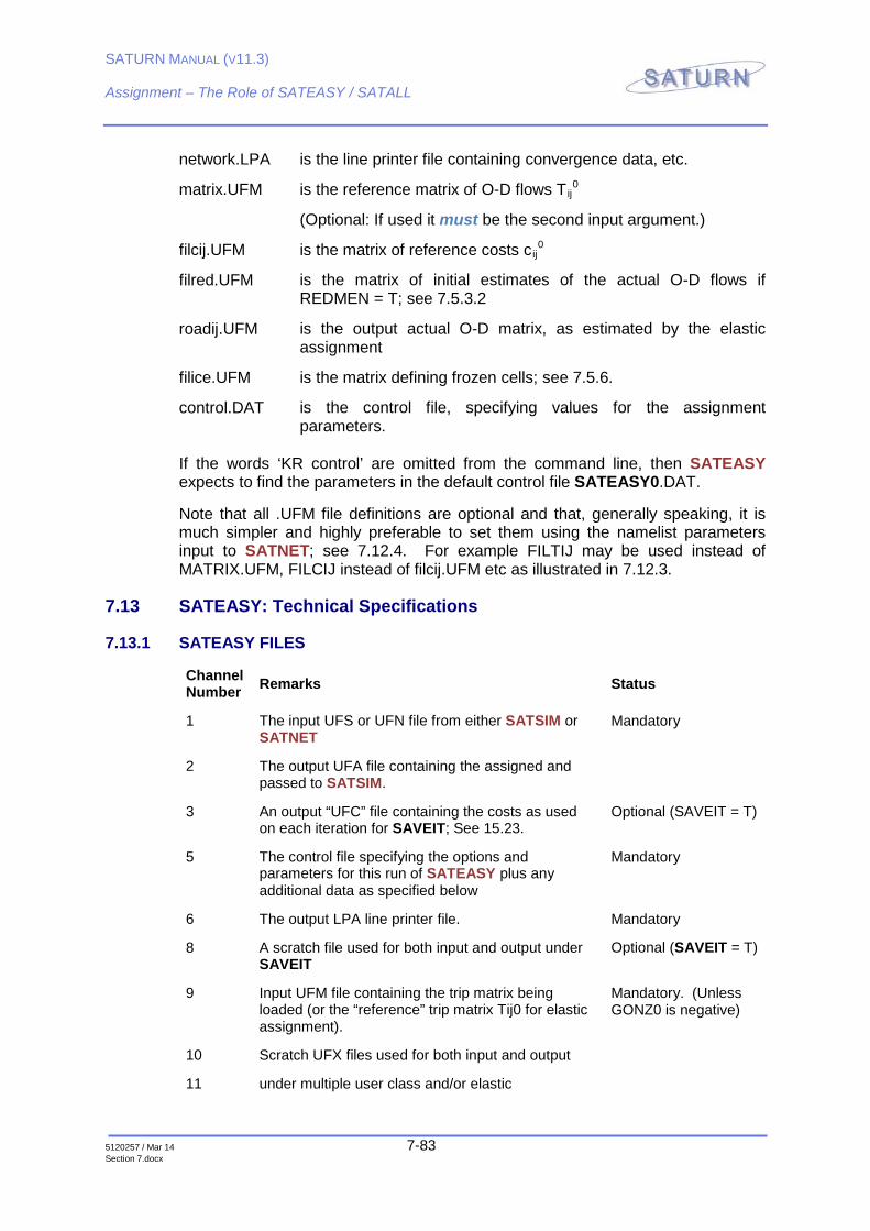
SATURN MANUAL (V11.3)
Assignment – The Role of SATEASY / SATALL
5120257 / Mar 14 7-83 Section 7.docx
network.LPA is the line printer file containing convergence data, etc.
matrix.UFM is the reference matrix of O-D flows Tij0
(Optional: If used it must be the second input argument.)
filcij.UFM is the matrix of reference costs cij0
filred.UFM is the matrix of initial estimates of the actual O-D flows if REDMEN = T; see 7.5.3.2
roadij.UFM is the output actual O-D matrix, as estimated by the elastic assignment
filice.UFM is the matrix defining frozen cells; see 7.5.6.
control.DAT is the control file, specifying values for the assignment parameters.
If the words ‘KR control’ are omitted from the command line, then SATEASY expects to find the parameters in the default control file SATEASY0.DAT.
Note that all .UFM file definitions are optional and that, generally speaking, it is much simpler and highly preferable to set them using the namelist parameters input to SATNET; see 7.12.4. For example FILTIJ may be used instead of MATRIX.UFM, FILCIJ instead of filcij.UFM etc as illustrated in 7.12.3.
7.13 SATEASY: Technical Specifications
7.13.1 SATEASY FILES
Channel Number Remarks Status
1 The input UFS or UFN file from either SATSIM or SATNET
Mandatory
2 The output UFA file containing the assigned and passed to SATSIM.
3 An output “UFC” file containing the costs as used on each iteration for SAVEIT; See 15.23.
Optional (SAVEIT = T)
5 The control file specifying the options and parameters for this run of SATEASY plus any additional data as specified below
Mandatory
6 The output LPA line printer file. Mandatory
8 A scratch file used for both input and output under SAVEIT
Optional (SAVEIT = T)
9 Input UFM file containing the trip matrix being loaded (or the “reference” trip matrix Tij0 for elastic assignment).
Mandatory. (Unless GONZ0 is negative)
10 Scratch UFX files used for both input and output
11 under multiple user class and/or elastic
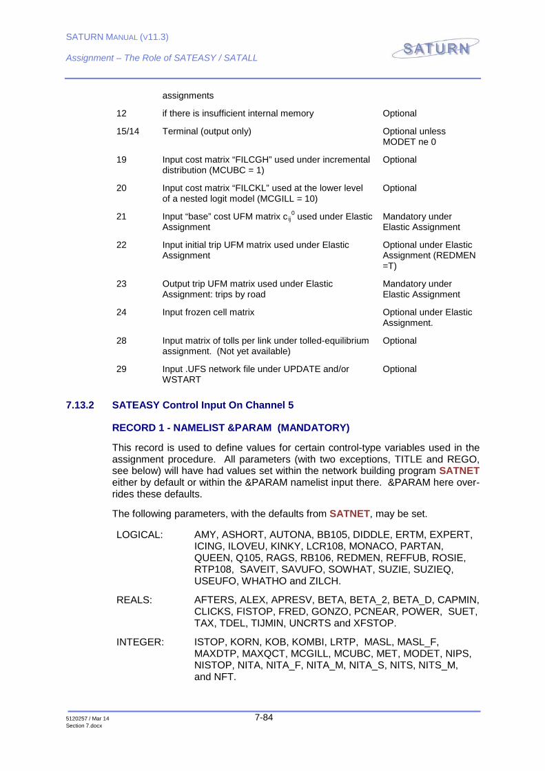
SATURN MANUAL (V11.3)
Assignment – The Role of SATEASY / SATALL
5120257 / Mar 14 7-84 Section 7.docx
assignments
12 if there is insufficient internal memory Optional
15/14 Terminal (output only) Optional unless MODET ne 0
19 Input cost matrix “FILCGH” used under incremental distribution (MCUBC = 1)
Optional
20 Input cost matrix “FILCKL” used at the lower level of a nested logit model (MCGILL = 10)
Optional
21 Input “base” cost UFM matrix cij0 used under Elastic
Assignment Mandatory under Elastic Assignment
22 Input initial trip UFM matrix used under Elastic Assignment
Optional under Elastic Assignment (REDMEN =T)
23 Output trip UFM matrix used under Elastic Assignment: trips by road
Mandatory under Elastic Assignment
24 Input frozen cell matrix Optional under Elastic Assignment.
28 Input matrix of tolls per link under tolled-equilibrium assignment. (Not yet available)
Optional
29 Input .UFS network file under UPDATE and/or WSTART
Optional
7.13.2 SATEASY Control Input On Channel 5
RECORD 1 - NAMELIST &PARAM (MANDATORY)
This record is used to define values for certain control-type variables used in the assignment procedure. All parameters (with two exceptions, TITLE and REGO, see below) will have had values set within the network building program SATNET either by default or within the &PARAM namelist input there. &PARAM here over-rides these defaults.
The following parameters, with the defaults from SATNET, may be set.
LOGICAL: AMY, ASHORT, AUTONA, BB105, DIDDLE, ERTM, EXPERT, ICING, ILOVEU, KINKY, LCR108, MONACO, PARTAN, QUEEN, Q105, RAGS, RB106, REDMEN, REFFUB, ROSIE, RTP108, SAVEIT, SAVUFO, SOWHAT, SUZIE, SUZIEQ, USEUFO, WHATHO and ZILCH.
REALS: AFTERS, ALEX, APRESV, BETA, BETA_2, BETA_D, CAPMIN, CLICKS, FISTOP, FRED, GONZO, PCNEAR, POWER, SUET, TAX, TDEL, TIJMIN, UNCRTS and XFSTOP.
INTEGER: ISTOP, KORN, KOB, KOMBI, LRTP, MASL, MASL_F, MAXDTP, MAXQCT, MCGILL, MCUBC, MET, MODET, NIPS, NISTOP, NITA, NITA_F, NITA_M, NITA_S, NITS, NITS_M, and NFT.
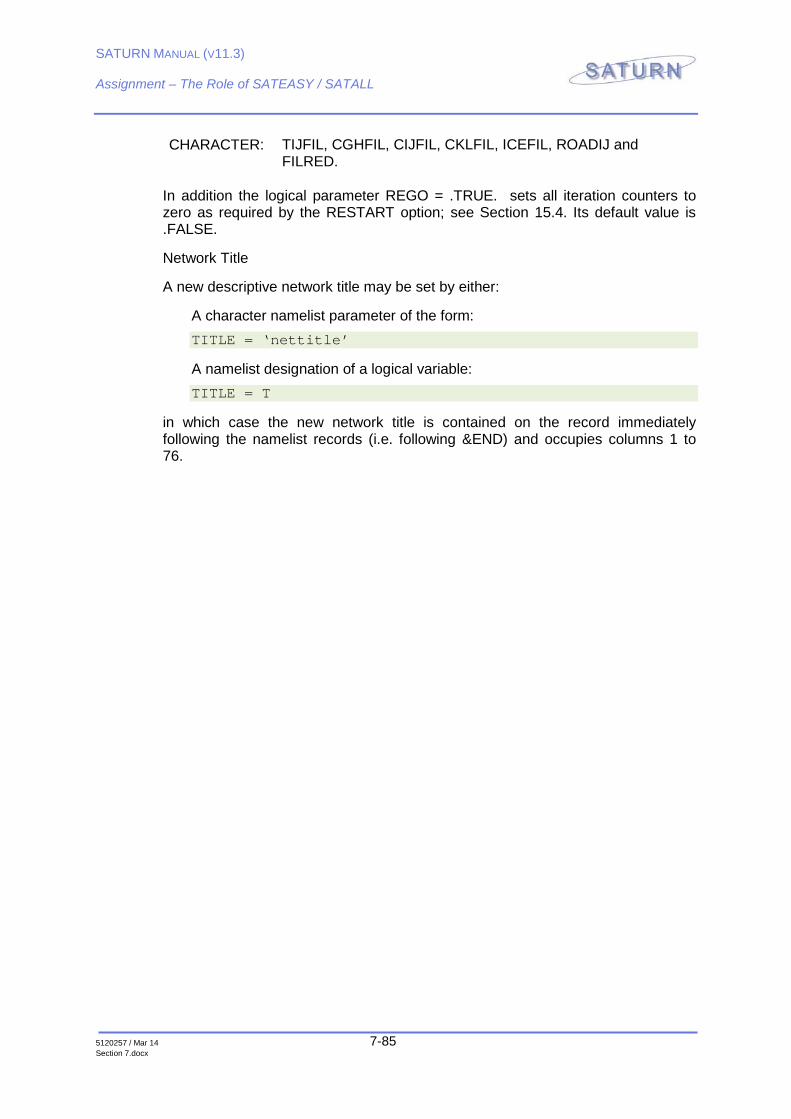
SATURN MANUAL (V11.3)
Assignment – The Role of SATEASY / SATALL
5120257 / Mar 14 7-85 Section 7.docx
CHARACTER: TIJFIL, CGHFIL, CIJFIL, CKLFIL, ICEFIL, ROADIJ and FILRED.
In addition the logical parameter REGO = .TRUE. sets all iteration counters to zero as required by the RESTART option; see Section 15.4. Its default value is .FALSE.
Network Title
A new descriptive network title may be set by either:
A character namelist parameter of the form: TITLE = ‘nettitle’
A namelist designation of a logical variable: TITLE = T
in which case the new network title is contained on the record immediately following the namelist records (i.e. following &END) and occupies columns 1 to 76.
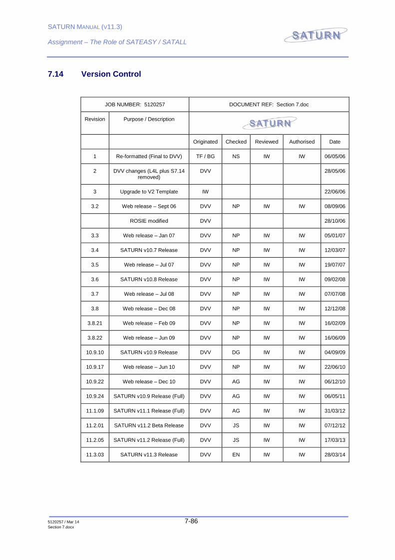
SATURN MANUAL (V11.3)
Assignment – The Role of SATEASY / SATALL
5120257 / Mar 14 7-86 Section 7.docx
7.14 Version Control
JOB NUMBER: 5120257 DOCUMENT REF: Section 7.doc
Revision Purpose / Description
Originated Checked Reviewed Authorised Date
1 Re-formatted (Final to DVV) TF / BG NS IW IW 06/05/06
2 DVV changes (L4L plus S7.14 removed)
DVV 28/05/06
3 Upgrade to V2 Template IW 22/06/06
3.2 Web release – Sept 06 DVV NP IW IW 08/09/06
ROSIE modified DVV 28/10/06
3.3 Web release – Jan 07 DVV NP IW IW 05/01/07
3.4 SATURN v10.7 Release DVV NP IW IW 12/03/07
3.5 Web release – Jul 07 DVV NP IW IW 19/07/07
3.6 SATURN v10.8 Release DVV NP IW IW 09/02/08
3.7 Web release – Jul 08 DVV NP IW IW 07/07/08
3.8 Web release – Dec 08 DVV NP IW IW 12/12/08
3.8.21 Web release – Feb 09 DVV NP IW IW 16/02/09
3.8.22 Web release – Jun 09 DVV NP IW IW 16/06/09
10.9.10 SATURN v10.9 Release DVV DG IW IW 04/09/09
10.9.17 Web release – Jun 10 DVV NP IW IW 22/06/10
10.9.22 Web release – Dec 10 DVV AG IW IW 06/12/10
10.9.24 SATURN v10.9 Release (Full) DVV AG IW IW 06/05/11
11.1.09 SATURN v11.1 Release (Full) DVV AG IW IW 31/03/12
11.2.01 SATURN v11.2 Beta Release DVV JS IW IW 07/12/12
11.2.05 SATURN v11.2 Release (Full) DVV JS IW IW 17/03/13
11.3.03 SATURN v11.3 Release DVV EN IW IW 28/03/14