7. instrumentation for noise measurements · 7. instrumentation for noise measurements ... voltage...

NOISE CONTROL Instrumentation 7.1

J.S. Lamancusa Penn State 12/4/2000

7. INSTRUMENTATION FOR NOISE MEASUREMENTS

7.1 PURPOSES OF MEASUREMENTS There are many reasons to make noise measurements. Noise data contains amplitude, frequency, time or phase information, which allows us to:

1. Identify and locate dominant noise sources 2. Optimize selection of noise control devices, methods, materials 3. Evaluate and compare noise control measures 4. Determine compliance with noise criteria and regulations 5. Quantify the strength (power) of a sound source 6. Determine the acoustic qualities of a room and its suitability for various uses

and many, many more…..

7.2 PERFORMANCE CHARACTERISTICS The performance characteristics of sound measurement instruments are quantified by: Frequency Response - Range of frequencies over which an instrument reproduces the correct amplitudes of the variable being measured (within acceptable limits). Typical Limits over a specified frequency range: Microphones ± 2dB Tape Recorders ± 1 or ± 3 dB Loudspeakers ± 5 dB Dynamic Range - Amplitude ratio between the maximum input level and the instrument’s internal “noise floor” (or self noise). All measurements should be at least 10 dB greater than the noise floor. The typical dynamic range of meters is 60 dB, more is better.


J.S. Lamancu

Response Time - The time interval required for an instrument to respond to a full scale input, (limited typically by output devices like meters, plotters) 7.2 SOUND LEVEL METERS The primary tool for noise measurement is the Sound Level Meter (SLM). The compromises with sound level meters are between accuracy, features and cost. The precision of a meter is quantified by its type (see standards IEC 651-1979, or ANSI S1.4-1983 for more details) Type 0 Laboratory reference standard, intended entirely fo

level meters Type 1 Precision sound level meter, intended for laborato

the acoustical environment can be closely cont~$5000)

Type 2 General purpose, intended for general field use adata for later frequency analysis (~$500)

Type 3 Survey meter, intended for preliminary invdetermination of whether noise environments are Shack)

Table 7.1 Principal allowable dB tolerance limits on

ANSI S1.4-1983)

Characteristic Type 0 Type 1Accuracy at calibration frequency to reference sound level

±0.4 dB ±0.7 dB

Accuracy of complete instrument for random incidence sound

±0.7 ±1.0

Maximum variation of level when the incidence angle is varied by ±22.5°

±0.5 (31-2000 Hz) ±1.5 (5000-6300 Hz) ±3 (10000-12500 Hz)

±1.0 (31-2000 H+2.5, -2 (500Hz) +4, -6.5 (10000Hz)

Maximum allowable variation of sound level for all angles of incidence

±1.0 (31-2000 Hz) ±1.5 (5000-6300 Hz) ±3 (10000-12500 Hz)

+1.5, -1(31-200±4 (5000-6300 H+8, -11 (10000Hz)

* none specified The most basic SLM will have an analog or digital output of sound pressure. Additional features can include octave or 1weighting networks (A,C, D, Lin), time averaging, and interfand plotting.

sa Penn State 12/4/2000

r calibration of other sound

ry use or for field use where rolled. (ballpark estimate:

nd for recording noise level

estigations such as the unduly bad. (~$50, Radio

sound level meters (ref

Type 2 ±1.0 dB

±1.5

z) 0-6300

-12500

±2.0 (31-2000 Hz) ±3.5 (5000-6300 Hz) * (10000-12500 Hz)

0 Hz) z)

-12500

±3(31-2000 Hz) +5, -8 (5000-6300 Hz) * (10000-12500 Hz)

A-weighted (or unweighted) /3 octave filters, frequency ace to a PC for data storage



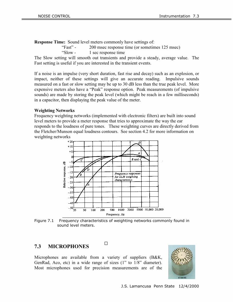
Response Time: Sound level meters commonly have settings of: “Fast” - 200 msec response time (or sometimes 125 msec) “Slow - 1 sec response time The Slow setting will smooth out transients and provide a steady, average value. The Fast setting is useful if you are interested in the transient events. If a noise is an impulse (very short duration, fast rise and decay) such as an explosion, or impact, neither of these settings will give an accurate reading. Impulsive sounds measured on a fast or slow setting may be up to 30 dB less than the true peak level. More expensive meters also have a “Peak” response option. Peak measurements (of impulsive sounds) are made by storing the peak level (which might be reach in a few milliseconds) in a capacitor, then displaying the peak value of the meter. Weighting Networks Frequency weighting networks (implemented with electronic filters) are built into sound level meters to provide a meter response that tries to approximate the way the ear responds to the loudness of pure tones. These weighting curves are directly derived from the Fletcher/Munson equal loudness contours. See section 4.2 for more information on weighting networks

Figure 7.1 Frequency characteristics of weighting networks commonly found in

sound level meters. 7.3 MICROPHONES Microphones are available from a variety of suppliers (B&K, GenRad, Aco, etc) in a wide range of sizes (1” to 1/8” diameter). Most microphones used for precision measurements are of the



condenser type. The construction of a condenser microphone is shown in Figure 7.2.

Figure 7.2 Schematic and cutaway views of a typical condenser microphone The basic operating principle for a condenser microphone is: a thin diaphragm and the fixed back plate, separated by a thin air gap, form the two plates of a capacitor. Pressure fluctuations from incoming sound waves cause the diaphragm to vibrate, changing the air gap. This changes the capacitance, which is measured electronically and converted into a voltage by appropriate circuitry, usually contained in a separate unit called a pre-amplifier. Instrumentation grade microphones are specially designed to have negligible sensitivity to temperature and humidity, and have excellent long term stability (see Table 7.2). Table 7.2 Specifications of general purpose B&K condenser microphones Size 1/8” 1/4” ½” 1” Model 4138 4135 4133 4145 Frequency response (± 2 dB) 6.5-140KHz 4-100KHz 4-40KHz 2.6-18KHz Sensitivity (mV/Pa) 1.0 4.0 12.5 50 Temperature Coefficient (dB/°C) -.01 -.01 -.002 -.002 Expected Long Term Stability at 20°C

>600 years/dB

>1000 years/dB

>1000 years/dB

Microphone selection depends on two primary parameters:

• Sensitivity - ratio of microphone output voltage to input pressure amplitude (in units of mV/Pa). In general, larger microphones have a greater sensitivity.

• Frequency Response - variation in sensitivity as a function of frequency (the

ideal is a perfectly flat response). Frequency response is specified as a range over which the output signal deviates less than ±2 dB. Typical frequency response curves are shown in Figure 7.3. Smaller microphones have a wider frequency response. At high frequencies (when wavelength approaches the diameter of the microphone) diffraction effects occur which alter the frequency response. These effects are dependent on the incidence angle of the sound waves (see Figure 7.4).


The frequency response curve approaches flat for 90 degrees (grazing) incidence. Each microphone is supplied with calibration curves, which can be used to compensate for this diffraction effect at high frequencies (but most people don’t). To minimize this error, use as small a microphone as possible.

Figure 7.3 Frequency re

an electrosta

Figure 7.4 Directional ch
1”
spotic

ar

1/2”

1/4"

1/8”


nse of B&K condenser microphones of various sizes using actuator

acteristics of ½” condenser microphone



Microphone types Pressure – designed to be used for coupler measurements, i.e. directly coupled to a test chamber Random (diffuse field) – designed to give optimum frequency response for random incidence sound (equal probability of sound from all directions, such as in a reverberant chamber) Free Field - designed to give optimum frequency response for sound from a particular incidence angle (usually 0 degrees)

Figure 7.5 Microphone orientation



7.5 FREQUENCY ANALYSIS (1/n Octave)

The most basic measurement any sound level meter can make is an overall dB level. This is a single number, which represents the sound energy over the entire frequency range of the meter. It provides no information about the frequency content of the sound. We can obtain information on the frequency content by using filters. The most common are octave band and 1/3 octave band filters. The most frequency detail is provided by FFT analysis. Octave Band - Measures the total acoustical energy within the passband of a band pass filter. The term “octave” denotes a doubling in frequency. Hence, each octave band covers a frequency range of one octave. We refer to the octave band by its center frequency. The center frequencies of successive filters are separated by one octave. The preferred octave band center frequencies (by international standard) are: 31.5, 63, 125, 250, 500, 1000, 2000, 4000, 8000 and 16000 Hz. The shape of a typical octave filter is shown in Figure 7.4 below. The bandwidth of a filter is the width in frequency between the –3 dB points. This is an example of a constant percentage bandwidth filter. The width of octave filters progressively increases with frequency. When plotted on a log scale, the shape of the band response is independent of frequency. The output of a percentage bandwidth filter is: dB/Bandwidth

Figure 7.4 Characteristics of an octave band filter



An octave band filter is not a perfect bandpass filter (it is physically impossible to build one). There is a finite “rolloff” or skirt on each side of the band. As can be seen in Figure 7.5, adjacent filters overlap each other slightly.

Figure 7.5 Complete filter characteristics for a typical octave band filter set

1/1 Octave Filter Relationships:

cc fu

fl ff 2/12/1 2 2 == −

ii cc ff 21

=+

= center frequencies of adjacent filters

Hz point), dB 3- (tofrequency cutoffupper Hz point), dB 3- (tofrequency cutofflower

==

u

l

ff

One-third, one-tenth octave analysis - More detail is sometimes needed to obtain adequate frequency resolution, hence the need for bandwidths finer than one octave. The choice of filter bandwidth depends on the nature of the measured noise - is it broadband or does it have significant pure tones which you want to identify? Closely spaced pure tones will not be discovered by a wide bandwidth analysis. 1/3 octave - Each full octave is spanned by three 1/3 octave bands

1/3 Octave Filter Relationships: cc f

uf

l ff 6/16/1 2 2 == −

iii ccc fff 26.12 3/1

1==

+ = center frequencies of adjacent filters



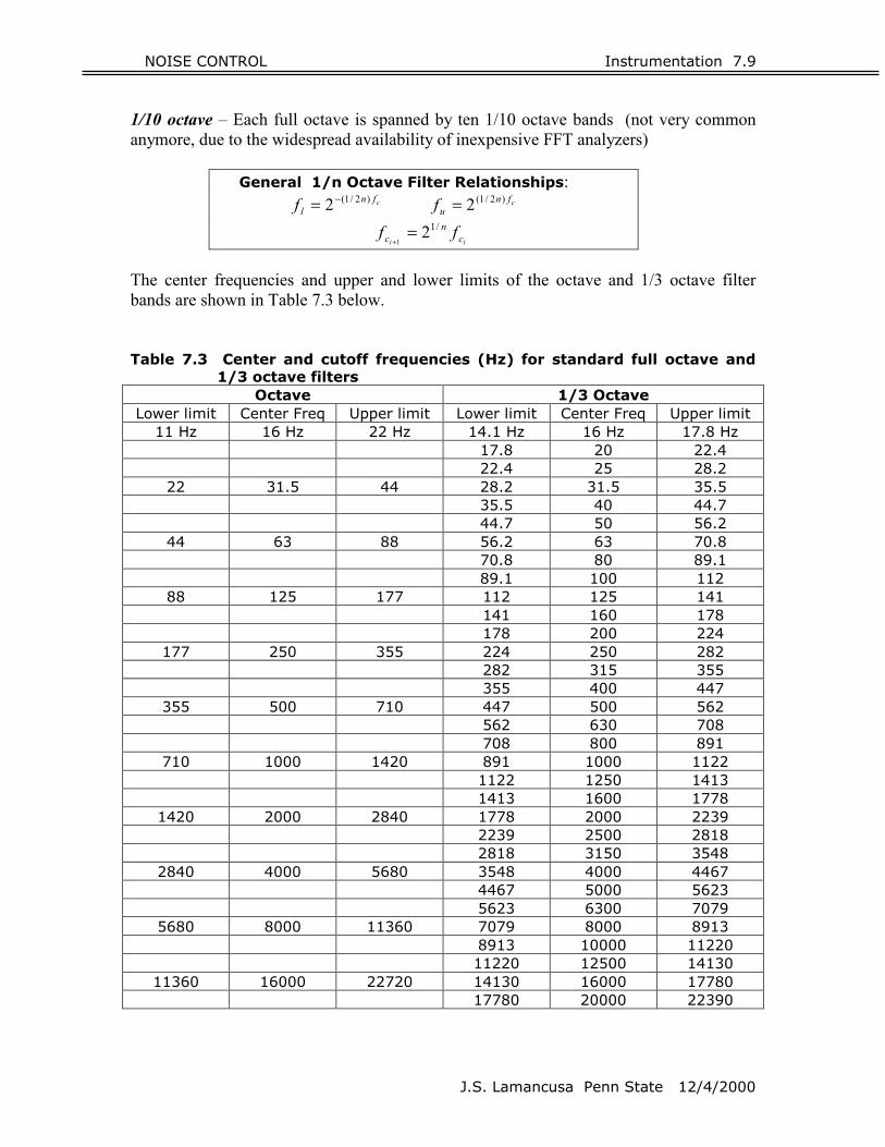
1/10 octave – Each full octave is spanned by ten 1/10 octave bands (not very common anymore, due to the widespread availability of inexpensive FFT analyzers)

General 1/n Octave Filter Relationships: cc fn

ufn

l ff )2/1()2/1( 2 2 == −

ii c

nc ff /12

1=

+

The center frequencies and upper and lower limits of the octave and 1/3 octave filter bands are shown in Table 7.3 below. Table 7.3 Center and cutoff frequencies (Hz) for standard full octave and

1/3 octave filters Octave 1/3 Octave

Lower limit Center Freq Upper limit Lower limit Center Freq Upper limit 11 Hz 16 Hz 22 Hz 14.1 Hz 16 Hz 17.8 Hz

17.8 20 22.4 22.4 25 28.2

22 31.5 44 28.2 31.5 35.5 35.5 40 44.7 44.7 50 56.2

44 63 88 56.2 63 70.8 70.8 80 89.1 89.1 100 112

88 125 177 112 125 141 141 160 178 178 200 224

177 250 355 224 250 282 282 315 355 355 400 447

355 500 710 447 500 562 562 630 708 708 800 891

710 1000 1420 891 1000 1122 1122 1250 1413 1413 1600 1778

1420 2000 2840 1778 2000 2239 2239 2500 2818 2818 3150 3548

2840 4000 5680 3548 4000 4467 4467 5000 5623 5623 6300 7079

5680 8000 11360 7079 8000 8913 8913 10000 11220 11220 12500 14130

11360 16000 22720 14130 16000 17780 17780 20000 22390



7.6 FFT ANALYSIS The FFT = Fast Fourier Transform, is a narrow band, constant bandwidth analysis (the frequency resolution does not change over the frequency range)

FFT refers to the numerical algorithm used to calculate the Fourier transform in “real time” (in less time than it takes to acquire the actual data). In layperson’s terms, the FFT determines the frequency content of a time signal. The mathematical definition of a Fourier transform is:

dtetxfX ftj�

+∞

∞−

−= π2)()(

The FFT algorithm discretizes this calculation. It requires a finite number of time data points, typically a power of 2, such as 512 (29) or 1024. It is a transformation from time to frequency.

Figure 7.6 The Fast Fourier Transform

Some sample time data (induction noise from a 2.5L 4 cylinder engine), and its associated frequency spectrum obtained by FFT are shown in Figure 7.7.

Figure 7.7 Induction noise data from a 4 cylinder engine running at 3000 RPM, wide

open throttle

FFTTIME DOMAIN: x(i∆t) = amplitude at time intervals of ∆t (seconds), N data samples

FREQUENCY DOMAIN: X(j∆f) = amplitude (complex) at frequency intervals of ∆f (Hz), ∆f =1/(N∆t) N/2 valid points

a) time history b) frequency spectrum



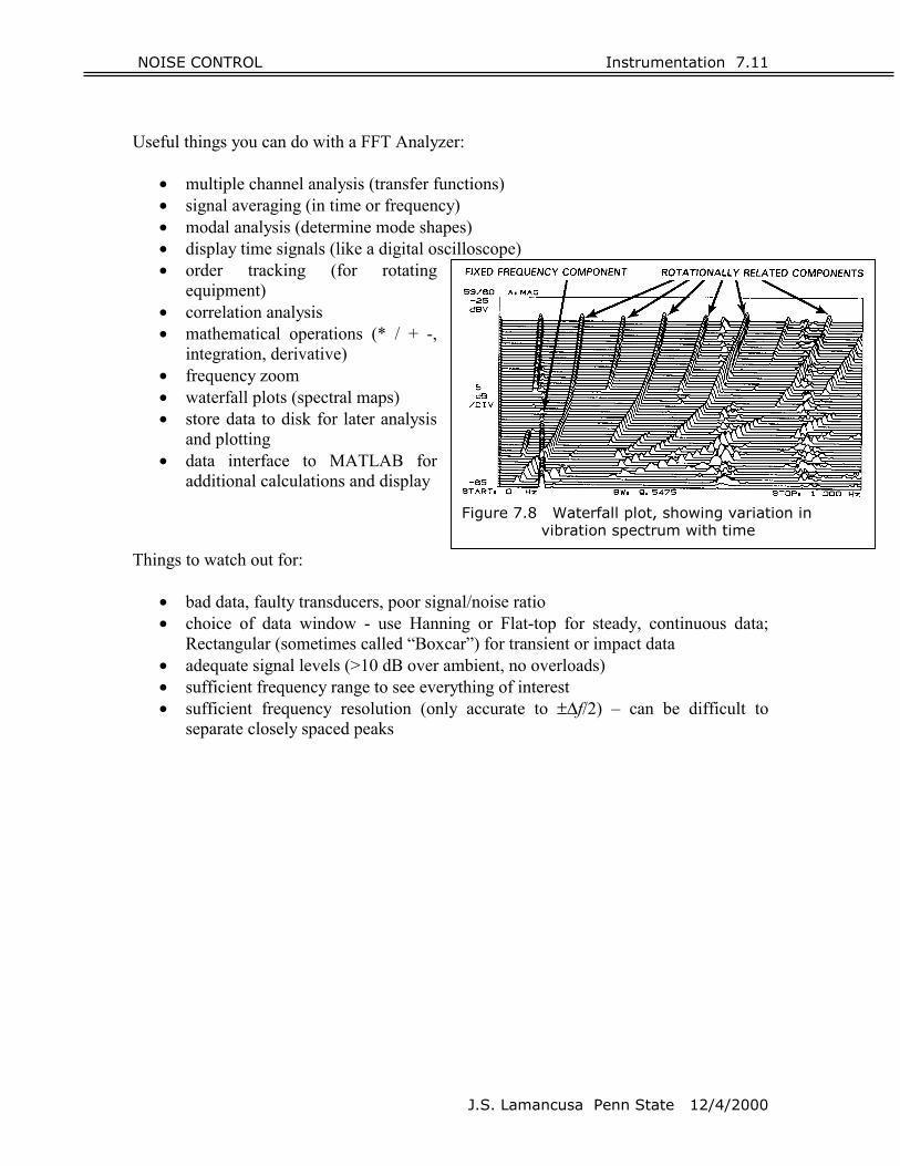
Useful things you can do with a FFT Analyzer:

• multiple channel analysis (transfer functions) • signal averaging (in time or frequency) • modal analysis (determine mode shapes) • display time signals (like a digital oscilloscope) • order tracking (for rotating

equipment) • correlation analysis • mathematical operations (* / + -,

integration, derivative) • frequency zoom • waterfall plots (spectral maps) • store data to disk for later analysis

and plotting • data interface to MATLAB for

additional calculations and display Things to watch out for:

• bad data, faulty transducers, poor signal/noise ratio • choice of data window - use Hanning or Flat-top for steady, continuous data;

Rectangular (sometimes called “Boxcar”) for transient or impact data • adequate signal levels (>10 dB over ambient, no overloads) • sufficient frequency range to see everything of interest • sufficient frequency resolution (only accurate to ±∆f/2) – can be difficult to

separate closely spaced peaks

Figure 7.8 Waterfall plot, showing variation in vibration spectrum with time



7.7 COMBINATION OF TWO OR MORE FREQUENCY BANDS A typical task is to determine the octave band level from 1/3 octave band measurements, or to calculate an overall level from individual octave or 1/3 octave bands. This is just like summing dB’s from several sources as in Section 6.1. The general expression for total pressure over the interval of interest is:

�� +++==

222

21

1

21

2 ... n

n

iT PPPPP

and in dB’s: ��==

=��

�

�

��

�

�=

��

�

�

��

�

� n

i

Ln

i ref

i

ref

T iP

PP

PP

1

10/10

2

110

2

10 10log10log10log10

The total power in an octave band is related to the individual 1/3 octave bands by:

23

22

21

2 PPPPoctave ++= (because we are adding energy, which is proportional to P2)

dBP

PL ppp LLL

ref

octaveP ��

�� ++== 10/310/210/1 101010log10log10 102

2

10

Example 1: The levels in the 400, 500 and 630 Hz 1/3 octave bands measure 72, 74, 68 dB. What is the octave band level for the 500 Hz band?

( ) dB76101010log10 8.64.72.710 =++

Example 2: Calculate the overall level for the following octave band measurements:

(Answer: 102.6 dB) Center Freq dB

125 79 250 80 500 94 1000 100 2000 94 4000 94 8000 88

NOISE CONTROL Instrumentation 7.13 7.8 CONVERSION FROM ONE BANDWIDTH TO ANOTHER There may be cases where you acquire data with one width of filter, and you later find you really needed to know the level over a different bandwidth. If you recorded all the 1/3 octave bands, it’s easy to convert to full octaves, just logarithmically add the dB’s as shown in the last section. However, what if you only measured one 1/3 octave band, but you desperately need to know the level over that entire octave? You have lost some information, but if you assume that the energy is uniformly distributed over the entire band (and there are no pure tones), then you can still make an estimate: Figure 7.9 The output of a filte First, let us define: Spectrum level = Sound level (d We can relate spectrum level to l

where: P = rms pressure output o PSL = rms pressure in 1 H This implicitly assumes that thethe width of the band (i.e. thmeasurement from one bandwidt

1

221

22 f

fPP = where: P1 = rms p

P2 = rms p and in terms of sound pressure le

Example: the output of the 1measured using the 125 Hz full o

Prms2

Energy in band (output of filter with width f) is proportional to area under the curve

f


r is determined by the amplitude and the bandwidth

B) read by an ideal analyzer with a 1 Hz bandwidth

evels taken with other bandwidths by:

fPP SL22 =

f filter with bandwidth f z band

total energy in a given band is proportional to p2 times e area under the p2 curve). To convert a pressure h to a different bandwidth:

ressure output over bandwidth f1

ressure output over bandwidth f2

vel:

1

21012 log10

ffLL +=

00 Hz 1/3 octave band is 58 dB, how much would be ctave band?

NOISE CONTROL Instrumentation 7.14 Answer: assuming that the level is uniform over the entire octave band,

1

21012 log10

ffLL +=

dB638.458

13log1058 10 =+=+=

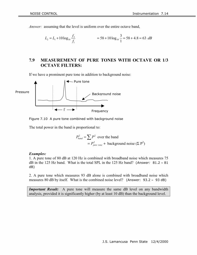
7.9 MEASUREMENT OF PURE TONES WITH OCTAVE OR 1/3

OCTAVE FILTERS: If we have a prominent pure tone in addition to background noise: Figure 7.10 A pure The total power in th

Examples: 1. A pure tone of 80 dB in the 125 Hz bandB) 2. A pure tone whicmeasures 80 dB by it Important Result: analysis, provided it i

Pressure

Frequency

e

Pure tone

f

tone combined wi

e band is proportio

�=2Pband

=

dB at 120 Hz is cod. What is the tot

h measures 93 dBself. What is the c

A pure tone wills significantly high

Background nois


th background noise

nal to:

2P over the band

+2tonepureP background noise (Σ P2)

mbined with broadband noise which measures 75 al SPL in the 125 Hz band? (Answer: 81.2 ≈ 81

alone is combined with broadband noise which ombined noise level? (Answer: 93.2 ≈ 93 dB)

measure the same dB level on any bandwidth er (by at least 10 dB) than the background level.



7.10 SYNTHESIZING OCTAVE OR 1/3 OCTAVE BANDS FROM DISCRETE FFT DATA

We can use an FFT analyzer to measure and record a noise spectrum (the sound pressure amplitude at discrete, evenly spaced intervals of frequency, ∆f). In some situations, it might be convenient to not have to haul around an octave band sound level meter too, so is there a way that we can use the FFT data to construct or “synthesize” the octave band data? The answer is a qualified “yes”. Each FFT data point represents the output of a filter which is ∆f Hz wide. The overall energy over a frequency band larger than ∆f is proportional to the area under the Prms

2 curve:

�=

=n

iiBAND PP

1

22

where: Pi

2 = mean square acoustic pressure of the ith FFT data point

n = number of FFT data points that fall within the bandwidth of the synthesized filter (see Table 7.2 for octave and 1/3 octave limits)

∆f = FFT frequency increment or “bin” size (Hz)

and in dB’s: log10=BANDdB �=

n

iiP

1

2

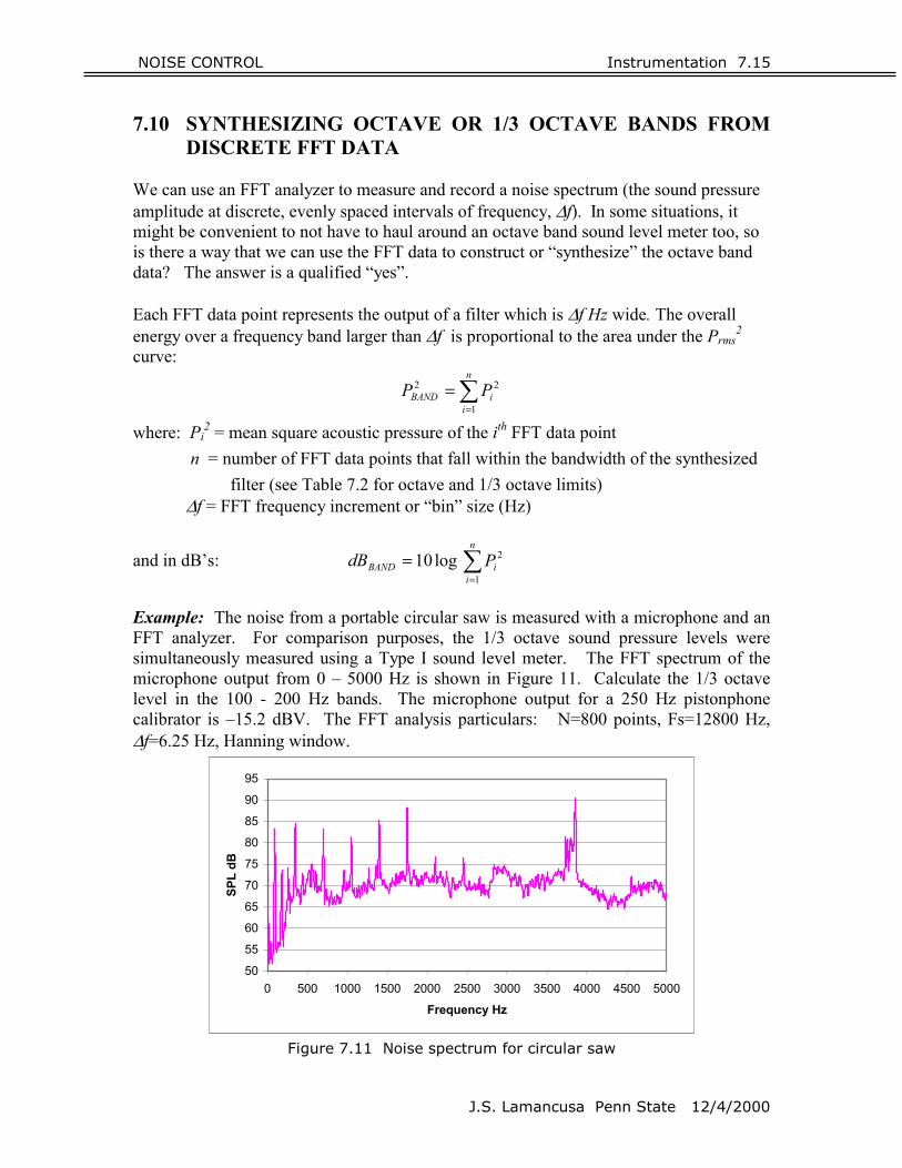
Example: The noise from a portable circular saw is measured with a microphone and an FFT analyzer. For comparison purposes, the 1/3 octave sound pressure levels were simultaneously measured using a Type I sound level meter. The FFT spectrum of the microphone output from 0 – 5000 Hz is shown in Figure 11. Calculate the 1/3 octave level in the 100 - 200 Hz bands. The microphone output for a 250 Hz pistonphone calibrator is –15.2 dBV. The FFT analysis particulars: N=800 points, Fs=12800 Hz, ∆f=6.25 Hz, Hanning window.

50

55

60

65

70

75

80

85

90

95

0 500 1000 1500 2000 2500 3000 3500 4000 4500 5000

Frequency Hz

SPL

dB

Figure 7.11 Noise spectrum for circular saw



Table 7.4 Partial FFT data for Circular Saw

Frequency (Hz) Microphone Output- dBV

Calibrated DB SPL

Synthesized dB Measured dB

81.25 -61.64 67.68

87.50 -47.08 82.24

93.75 -46.08 83.24

100.00 -58.03 71.29 83.5 83.2

106.25 -72.53 56.79

112.50 -74.97 54.35

118.75 -73.90 55.42

125.00 -73.78 55.54 62.6 61.3

131.25 -73.73 55.59

137.50 -72.51 56.81

143.75 -73.05 56.27

150.00 -73.33 55.99

156.25 -72.97 56.35

162.50 -67.07 62.25 70.1 70.2

168.75 -64.37 64.95

175.00 -63.12 66.20

181.25 -55.79 73.53

187.50 -59.01 70.31

193.75 -71.64 57.68

200.00 -73.54 55.78 75.7 75.1

206.25 -70.26 59.06

212.50 -67.87 61.45

218.75 -68.99 60.33

225.00 -68.64 60.68

231.25 -67.33 61.99

The major problem with this approach is for the lower frequency bands. Since FFT’s provide data at equal frequency intervals, the lowest octave bands may only encompass a few FFT points. This will degrade the accuracy of the “synthesized” band calculation.


J.S. Lamanc

7.11 WHITE NOISE AND PINK NOISE White noise is defined as having the same amplitude at all frequencies (radio static, or a jet of compressed air are pretty good approximations). It is often used as a known input to a system, in order to determine the system’s frequency response. What happens when white noise is measured using an octave band filter system? Octave band i Figure 7.12 White (random) noise has constant amplitu

The energy (and SPL) in band i is proportional to the area unEach succeeding octave band doubles in width, thereforeeach succeeding band. This results in an increase in SPsuccessive octave band as displayed in Figure 13. Figure 7.13 Output of octave band filters to white nooctave band increases by 3dB Pink noise is specifically designed to yield constant amplOn a linear scale, it decreases in amplitude as frequency inc(-3 dB/octave) to compensate for the increasing widths of th

Mean Square Pressure Prms

2(f)

e

Octave band i Octave band i+1, Twice as wide as band i

fi fi+1

z

Ideal white nois

de at all frequencies

der the curve: irms fP 2 the total energy doubles for L of 3dB (10log2) for each

Frequency (linear scale)

+3dB/octave

63 125 250 500 1K 2K H

usa Penn State 12/4/2000

ise input - each successive

itude across all octave bands. reases in just the right amount e octave filters.



7.12 SOUND LEVEL METER OR FFT ANALYZER? So which do you use? It depends on the application, and your budget. Here’s a qualitative comparison: Table 7.5 Comparison of Sound Level Meter to FFT Analyzer Sound Level Meter (with octave band filters)

FFT Analyzer

minimal data (less to write down) Produces lots of data (need to plot or record on disk)

crude frequency analysis detailed frequency analysis, identification of noise sources

good for assessing compliance with regulations

can separate closely spaced sources

compact, portable, weather resistant bulky, heavy, fussy easy to learn, and use, limited features

complex, lots of features, storage, data manipulation

adequate for material selection useful for many other purposes (vibration, transfer function analysis, etc)

relatively inexpensive $500 to $3000 $5K-15K

7. instrumentation for noise measurements · 7. instrumentation for noise measurements ... voltage...

Documents