7 optimization in matlab - ulisboa optimization in matlab matlab (matrix labboratory) is a numerical...

7 Optimization in MATLAB

MATLAB (MAtrix LABboratory) is a numerical computing environment and fourth-generation

programming language developed by MathWorks R© [1].

MATLAB allows matrix manipulations, plotting of functions and data, implementation of

algorithms, creation of user interfaces, and interfacing with programs written in other languages,

including C, C++, Java, and Fortran.

MATLAB has five toolboxes relevant to this course, containing two of them optimization

algorithms discussed in this class:

• Optimization ToolboxTM

• Global Optimization ToolboxTM

• Curve Fitting ToolboxTM

• Neural Network ToolboxTM

• Statistics ToolboxTM

Multidisciplinary Design Optimization of Aircrafts 476

7.1 Optimization ToolboxTM

Optimization Algorithms

• Unconstrained Nonlinear Optimization

• Constrained Nonlinear Optimization

• Linear Programming

• Quadratic Programming

• Binary Integer Programming

• Least Squares (Model Fitting)

• Multiobjective Optimization


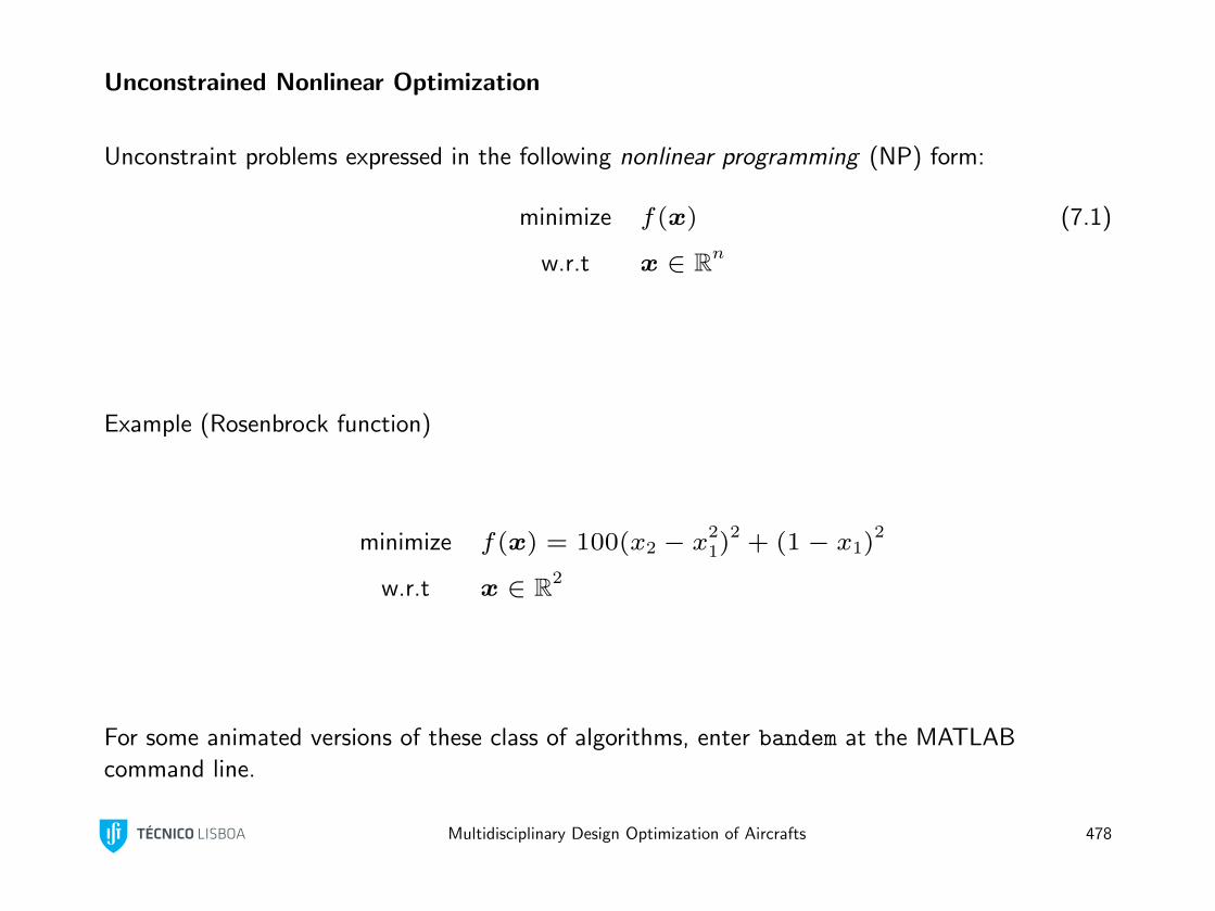
Unconstrained Nonlinear Optimization

Unconstraint problems expressed in the following nonlinear programming (NP) form:

minimize f(x) (7.1)

w.r.t x ∈ Rn

Example (Rosenbrock function)

minimize f(x) = 100(x2 − x21)

2+ (1− x1)

2

w.r.t x ∈ R2

For some animated versions of these class of algorithms, enter bandem at the MATLAB

command line.


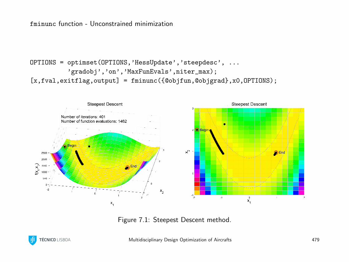
fminunc function - Unconstrained minimization

OPTIONS = optimset(OPTIONS,’HessUpdate’,’steepdesc’, ...

’gradobj’,’on’,’MaxFunEvals’,niter_max);

[x,fval,exitflag,output] = fminunc(@objfun,@objgrad,x0,OPTIONS);

Figure 7.1: Steepest Descent method.


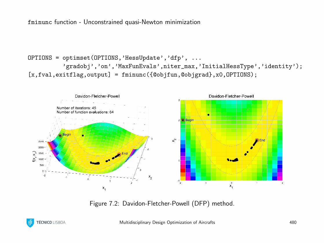
fminunc function - Unconstrained quasi-Newton minimization

OPTIONS = optimset(OPTIONS,’HessUpdate’,’dfp’, ...

’gradobj’,’on’,’MaxFunEvals’,niter_max,’InitialHessType’,’identity’);


Figure 7.2: Davidon-Fletcher-Powell (DFP) method.


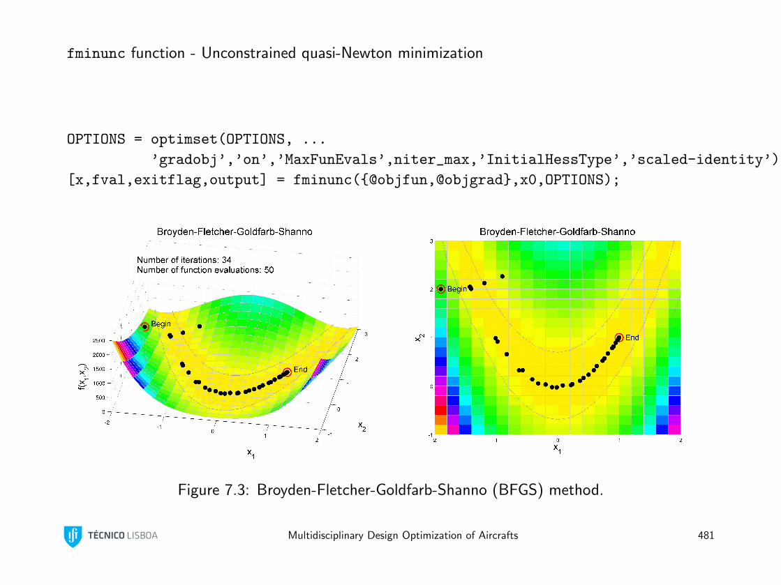
fminunc function - Unconstrained quasi-Newton minimization

OPTIONS = optimset(OPTIONS, ...

’gradobj’,’on’,’MaxFunEvals’,niter_max,’InitialHessType’,’scaled-identity’);


Figure 7.3: Broyden-Fletcher-Goldfarb-Shanno (BFGS) method.


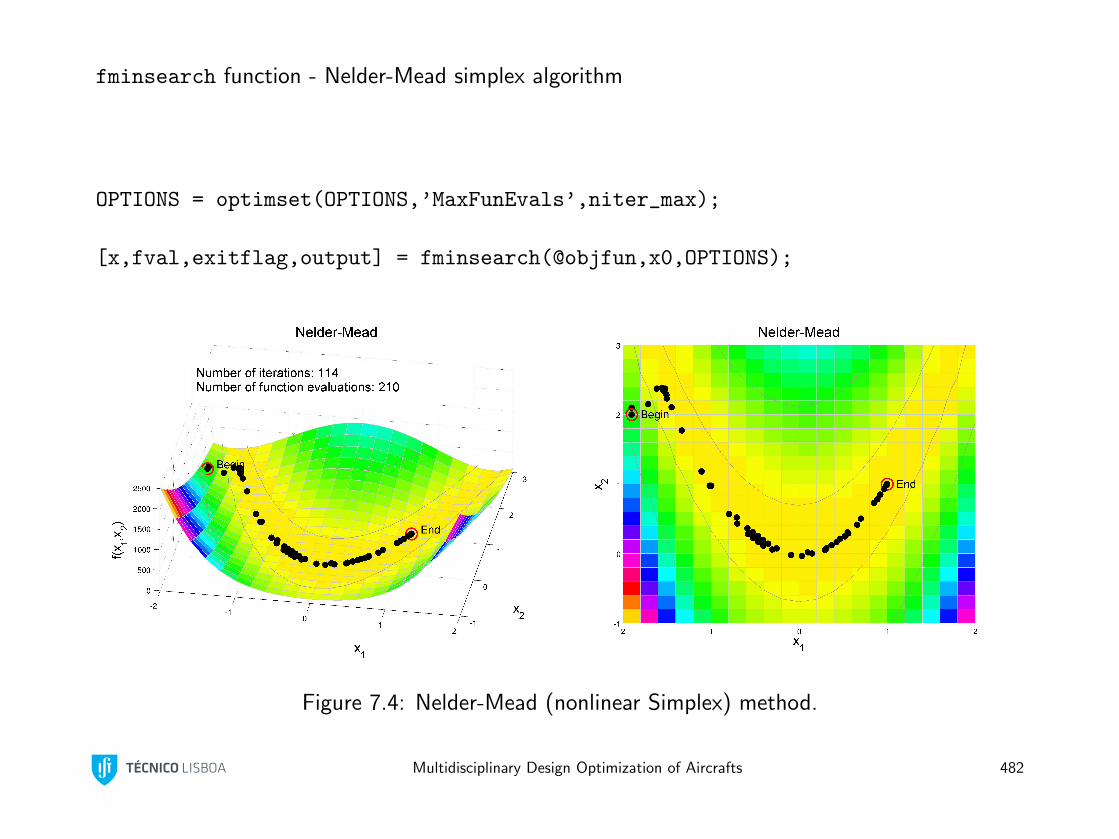
fminsearch function - Nelder-Mead simplex algorithm

OPTIONS = optimset(OPTIONS,’MaxFunEvals’,niter_max);

[x,fval,exitflag,output] = fminsearch(@objfun,x0,OPTIONS);

Figure 7.4: Nelder-Mead (nonlinear Simplex) method.


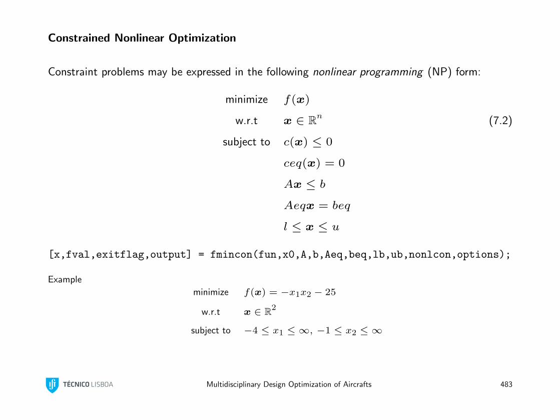
Constrained Nonlinear Optimization

Constraint problems may be expressed in the following nonlinear programming (NP) form:

minimize f(x)

w.r.t x ∈ Rn (7.2)

subject to c(x) ≤ 0

ceq(x) = 0

Ax ≤ b

Aeqx = beq

l ≤ x ≤ u

[x,fval,exitflag,output] = fmincon(fun,x0,A,b,Aeq,beq,lb,ub,nonlcon,options);

Example

minimize f(x) = −x1x2 − 25

w.r.t x ∈ R2

subject to −4 ≤ x1 ≤ ∞, −1 ≤ x2 ≤ ∞


fmincon function - Trust region algorithm

OPTIONS = optimset(OPTIONS,’Algorithm’,’trust-region-reflective’,...

’GradObj’,’on’);

[x,fval,exitflag,output] = fmincon(@objfun,@objgrad,x0,[],[],...

[],[],[x_min y_min],[+Inf +Inf],[],OPTIONS);

Figure 7.5: Trust region algorithm.


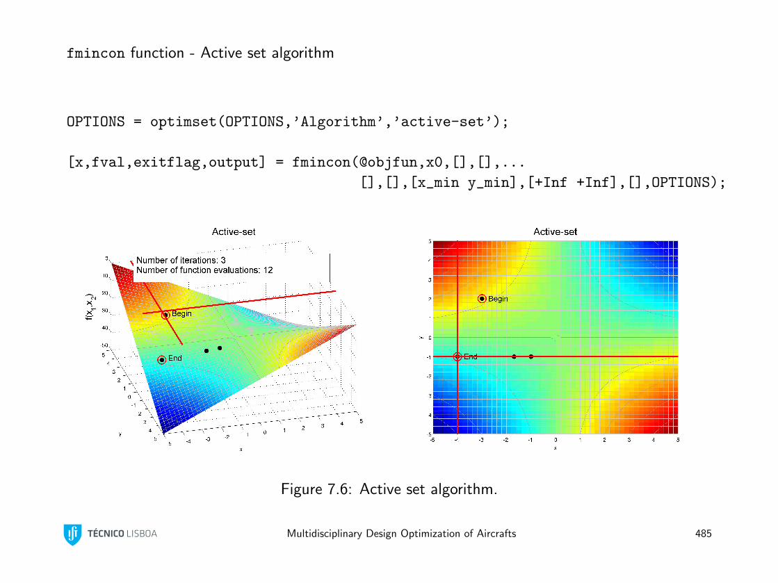
fmincon function - Active set algorithm

OPTIONS = optimset(OPTIONS,’Algorithm’,’active-set’);

[x,fval,exitflag,output] = fmincon(@objfun,x0,[],[],...


Figure 7.6: Active set algorithm.


fmincon function - Interior point algorithm

OPTIONS = optimset(OPTIONS,’Algorithm’,’interior-point’);

[x,fval,exitflag,output] = fmincon(objfun,x0,[],[],...


Figure 7.7: Interior point algorithm.


Linear Programming

linprog function - active set strategy (a.k.a. projection method)

linprog function - Simplex method


Quadratic Programming

quadprog function - Trust region algorithm

quadprog function - Active set algorithm

quadprog function - Interior point algorithm


Binary Integer Programming

bintprog function - Linear programming (LP)-based branch-and-bound algorithm


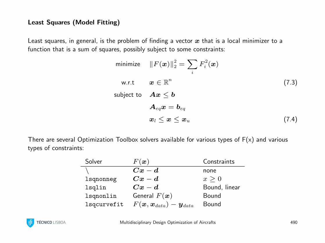
Least Squares (Model Fitting)

Least squares, in general, is the problem of finding a vector x that is a local minimizer to a

function that is a sum of squares, possibly subject to some constraints:

minimize ‖F (x)‖22 =

∑i

F2i (x)

w.r.t x ∈ Rn (7.3)

subject to Ax ≤ b

Aeqx = beq

xl ≤ x ≤ xu (7.4)

There are several Optimization Toolbox solvers available for various types of F(x) and various

types of constraints:

Solver F (x) Constraints

\ Cx− d none

lsqnonneg Cx− d x ≥ 0

lsqlin Cx− d Bound, linear

lsqnonlin General F (x) Bound

lsqcurvefit F (x,xdata)− ydata Bound


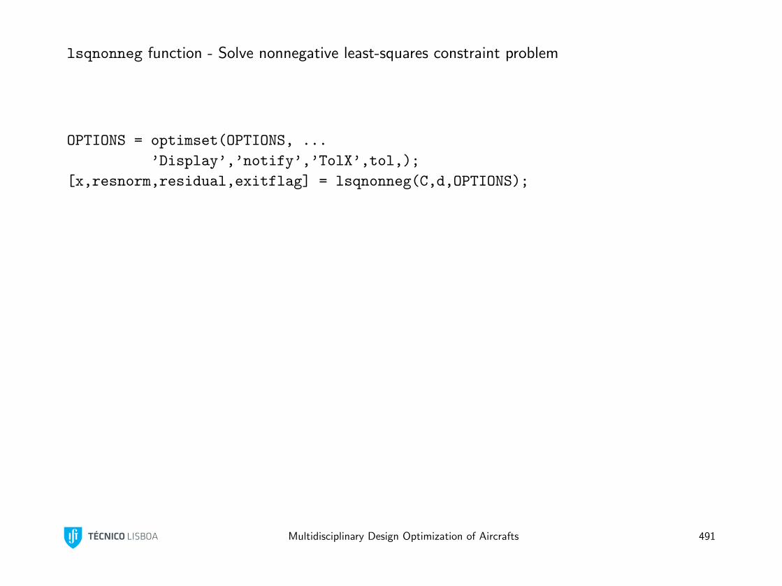
lsqnonneg function - Solve nonnegative least-squares constraint problem


’Display’,’notify’,’TolX’,tol,);

[x,resnorm,residual,exitflag] = lsqnonneg(C,d,OPTIONS);


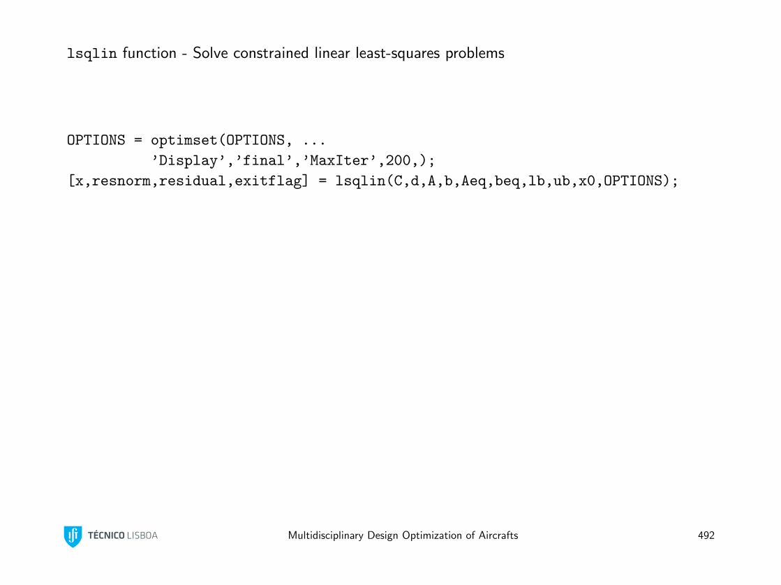
lsqlin function - Solve constrained linear least-squares problems


’Display’,’final’,’MaxIter’,200,);

[x,resnorm,residual,exitflag] = lsqlin(C,d,A,b,Aeq,beq,lb,ub,x0,OPTIONS);


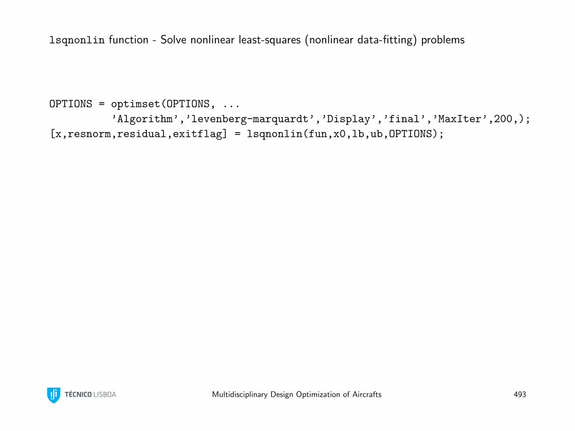
lsqnonlin function - Solve nonlinear least-squares (nonlinear data-fitting) problems


’Algorithm’,’levenberg-marquardt’,’Display’,’final’,’MaxIter’,200,);

[x,resnorm,residual,exitflag] = lsqnonlin(fun,x0,lb,ub,OPTIONS);


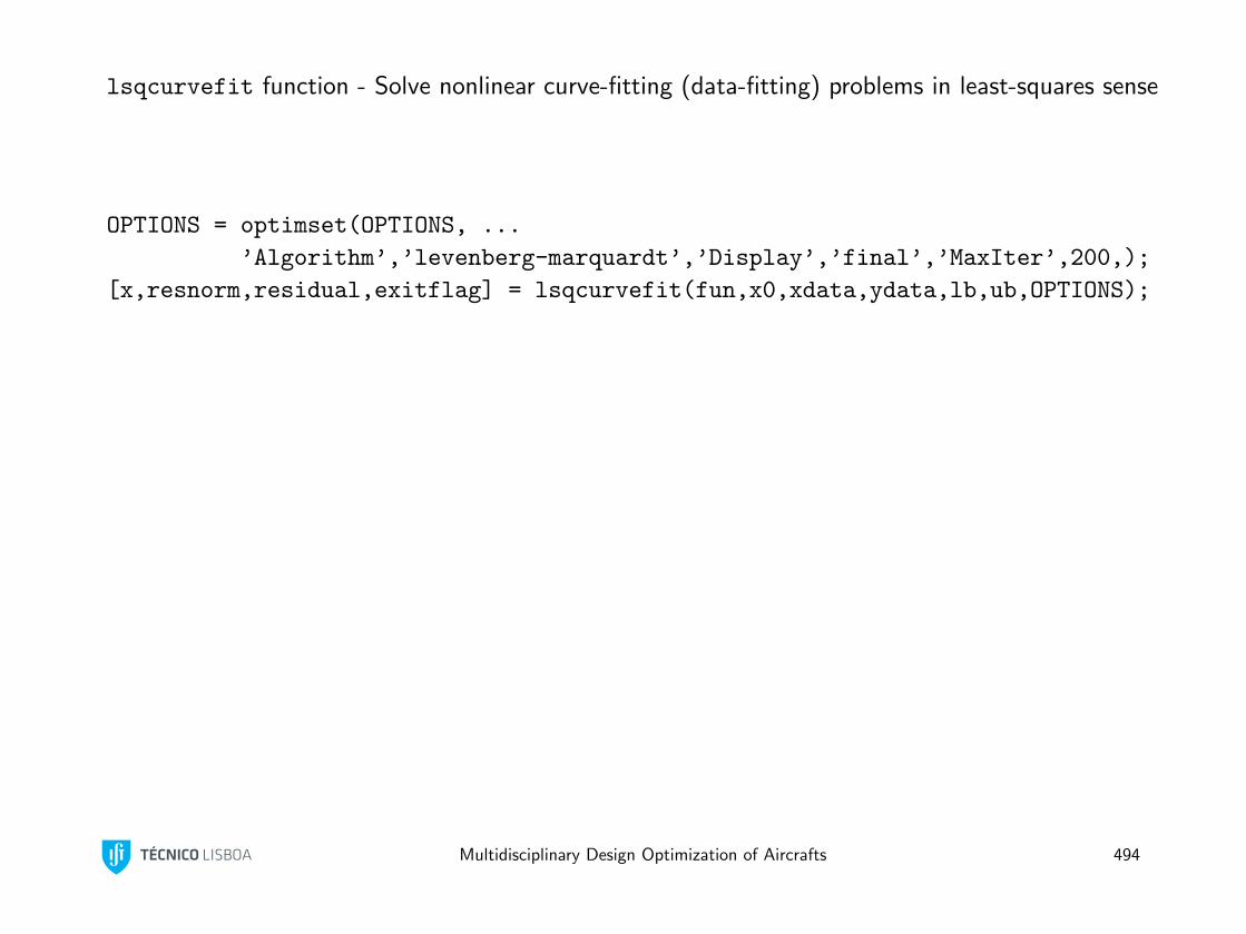
lsqcurvefit function - Solve nonlinear curve-fitting (data-fitting) problems in least-squares sense


’Algorithm’,’levenberg-marquardt’,’Display’,’final’,’MaxIter’,200,);

[x,resnorm,residual,exitflag] = lsqcurvefit(fun,x0,xdata,ydata,lb,ub,OPTIONS);


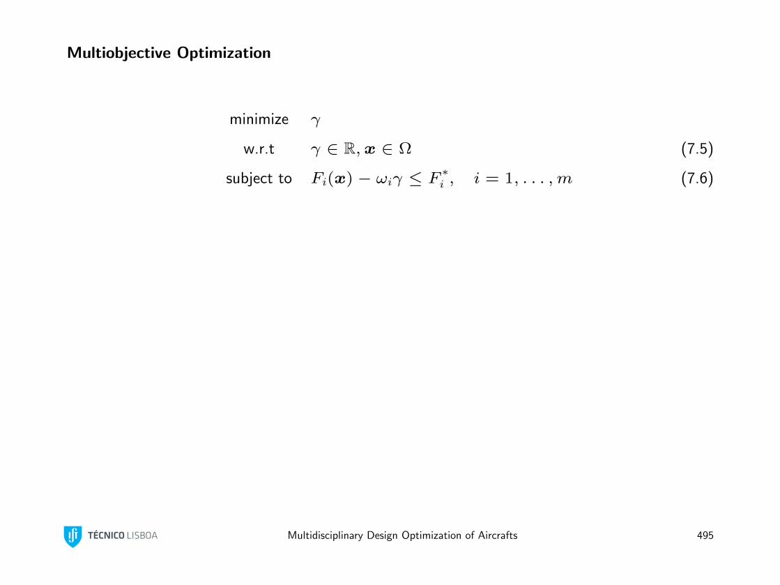
Multiobjective Optimization

minimize γ

w.r.t γ ∈ R,x ∈ Ω (7.5)

subject to Fi(x)− ωiγ ≤ F ∗i , i = 1, . . . ,m (7.6)


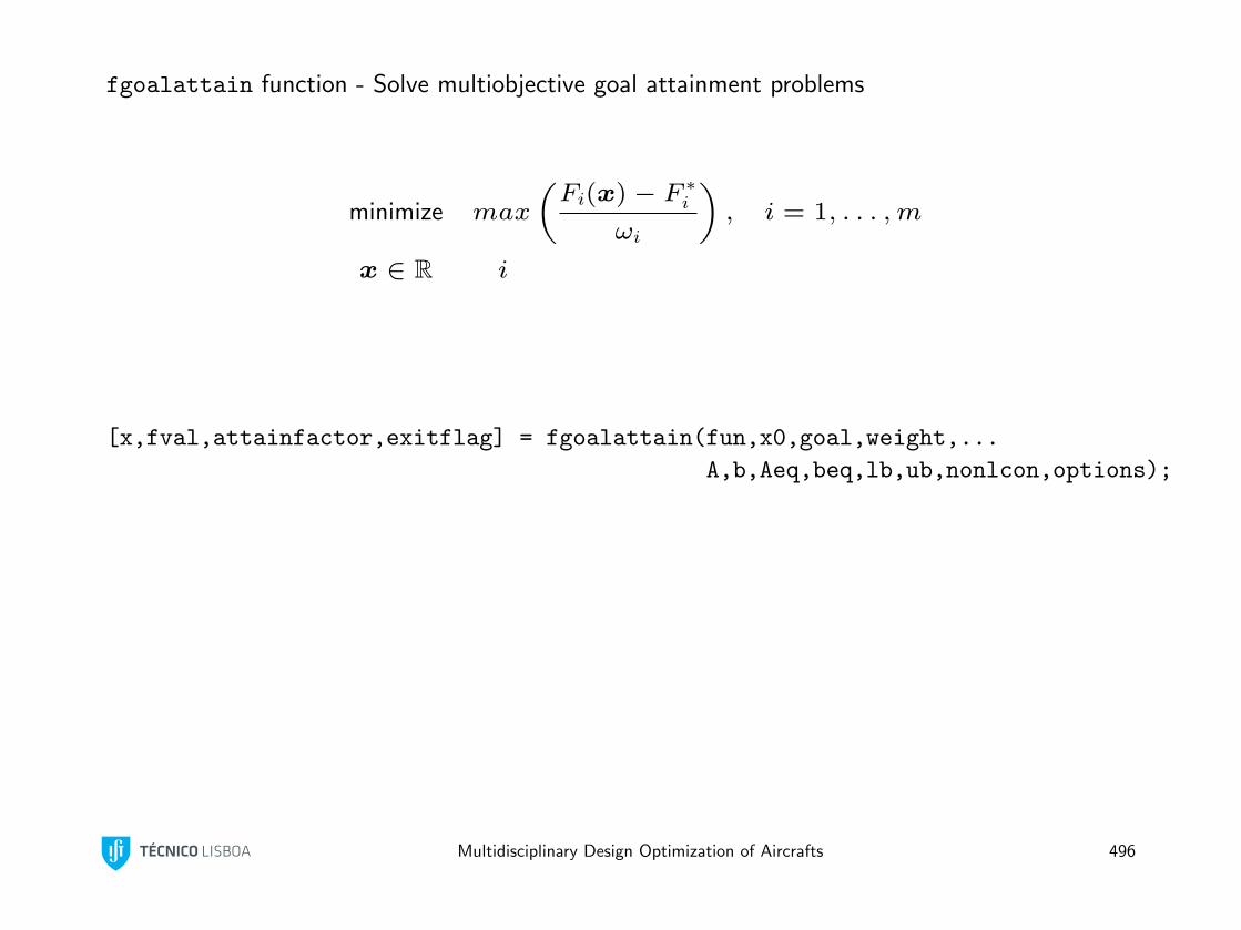
fgoalattain function - Solve multiobjective goal attainment problems

minimize max

(Fi(x)− F ∗i

ωi

), i = 1, . . . ,m

x ∈ R i

[x,fval,attainfactor,exitflag] = fgoalattain(fun,x0,goal,weight,...

A,b,Aeq,beq,lb,ub,nonlcon,options);


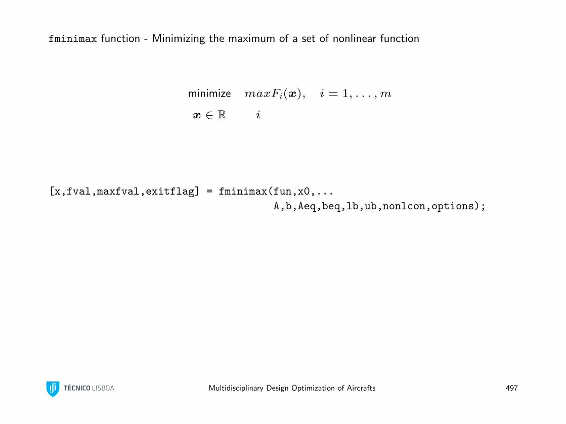
fminimax function - Minimizing the maximum of a set of nonlinear function

minimize maxFi(x), i = 1, . . . ,m

x ∈ R i

[x,fval,maxfval,exitflag] = fminimax(fun,x0,...

A,b,Aeq,beq,lb,ub,nonlcon,options);


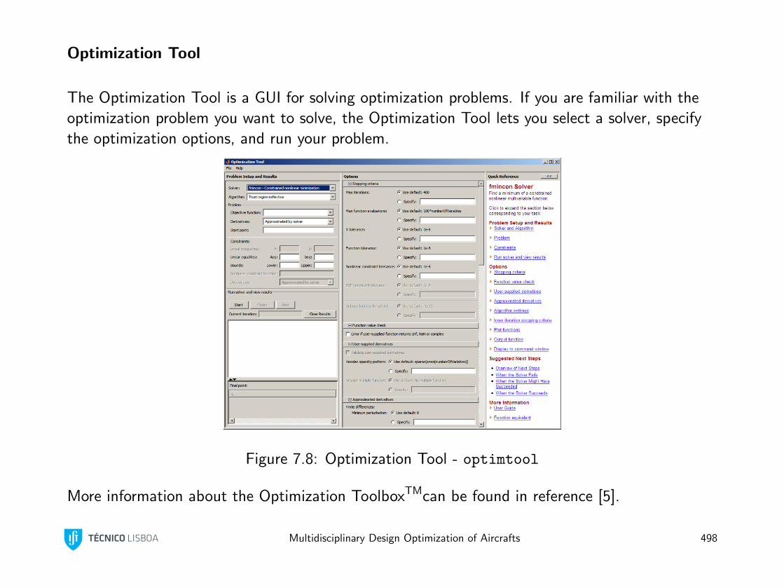
Optimization Tool

The Optimization Tool is a GUI for solving optimization problems. If you are familiar with the

optimization problem you want to solve, the Optimization Tool lets you select a solver, specify

the optimization options, and run your problem.

Figure 7.8: Optimization Tool - optimtool

More information about the Optimization ToolboxTMcan be found in reference [5].


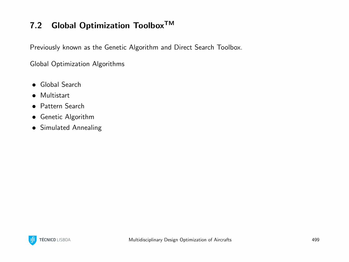
7.2 Global Optimization ToolboxTM

Previously known as the Genetic Algorithm and Direct Search Toolbox.

Global Optimization Algorithms

• Global Search

• Multistart

• Pattern Search

• Genetic Algorithm

• Simulated Annealing


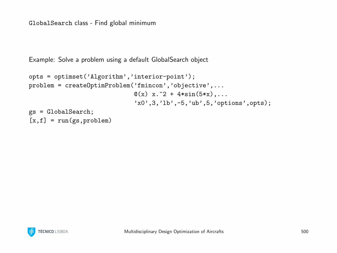
GlobalSearch class - Find global minimum

Example: Solve a problem using a default GlobalSearch object

opts = optimset(’Algorithm’,’interior-point’);

problem = createOptimProblem(’fmincon’,’objective’,...

@(x) x.^2 + 4*sin(5*x),...

’x0’,3,’lb’,-5,’ub’,5,’options’,opts);

gs = GlobalSearch;

[x,f] = run(gs,problem)


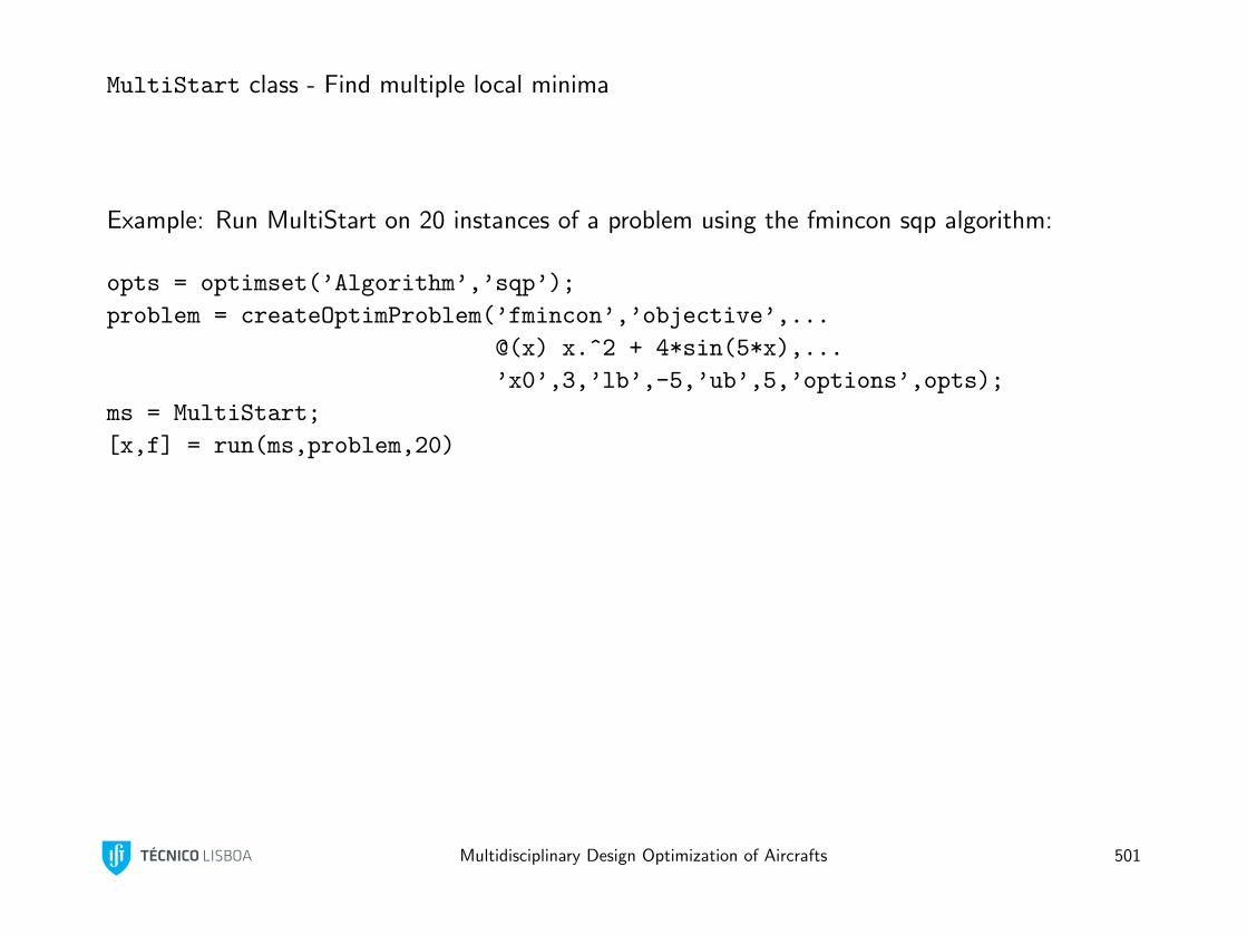
MultiStart class - Find multiple local minima

Example: Run MultiStart on 20 instances of a problem using the fmincon sqp algorithm:

opts = optimset(’Algorithm’,’sqp’);

problem = createOptimProblem(’fmincon’,’objective’,...

@(x) x.^2 + 4*sin(5*x),...

’x0’,3,’lb’,-5,’ub’,5,’options’,opts);

ms = MultiStart;

[x,f] = run(ms,problem,20)


ga function - Find minimum of function using genetic algorithm

[x,fval,exitflag,output] = ga(fitnessfcn,nvars,A,b,Aeq,beq,LB,UB,nonlcon,options);


gamultiobj function - Find minima of multiple functions using genetic algorithm

[x,fval,exitflag,output] = gamultiobj(fitnessfcn,nvars,A,b,Aeq,beq,LB,UB,options);


patternsearch function - Find minimum of function using pattern search

[x,fval,exitflag,output] = patternsearch(@fun,x0,A,b,Aeq,beq,LB,UB,nonlcon,options);


simulannealbnd function - Find unconstrained or bound-constrained minimum of function of

several variables using simulated annealing algorithm

[x,fval,exitflag,output] = simulannealbnd(fun,x0,lb,ub,options);

More information about the Global Optimization ToolboxTMcan be found in reference [3].


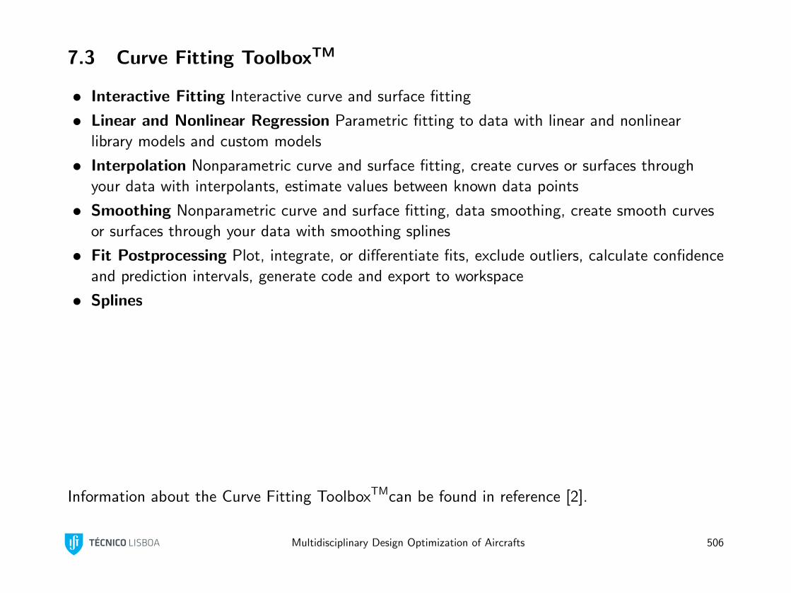
7.3 Curve Fitting ToolboxTM

• Interactive Fitting Interactive curve and surface fitting

• Linear and Nonlinear Regression Parametric fitting to data with linear and nonlinear

library models and custom models

• Interpolation Nonparametric curve and surface fitting, create curves or surfaces through

your data with interpolants, estimate values between known data points

• Smoothing Nonparametric curve and surface fitting, data smoothing, create smooth curves

or surfaces through your data with smoothing splines

• Fit Postprocessing Plot, integrate, or differentiate fits, exclude outliers, calculate confidence

and prediction intervals, generate code and export to workspace

• Splines

Information about the Curve Fitting ToolboxTMcan be found in reference [2].


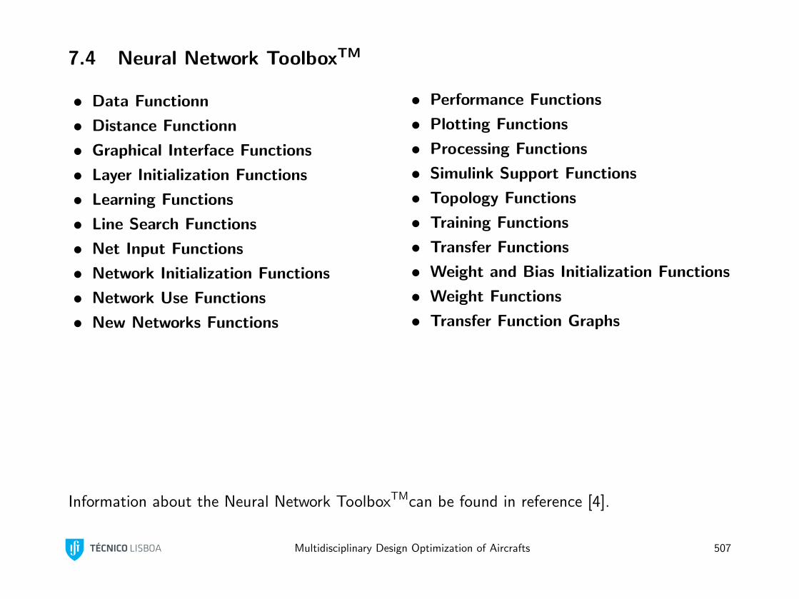
7.4 Neural Network ToolboxTM

• Data Functionn

• Distance Functionn

• Graphical Interface Functions

• Layer Initialization Functions

• Learning Functions

• Line Search Functions

• Net Input Functions

• Network Initialization Functions

• Network Use Functions

• New Networks Functions

• Performance Functions

• Plotting Functions

• Processing Functions

• Simulink Support Functions

• Topology Functions

• Training Functions

• Transfer Functions

• Weight and Bias Initialization Functions

• Weight Functions

• Transfer Function Graphs

Information about the Neural Network ToolboxTMcan be found in reference [4].


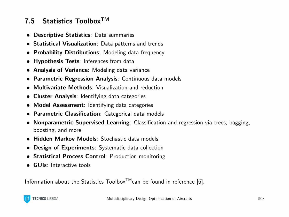
7.5 Statistics ToolboxTM

• Descriptive Statistics: Data summaries

• Statistical Visualization: Data patterns and trends

• Probability Distributions: Modeling data frequency

• Hypothesis Tests: Inferences from data

• Analysis of Variance: Modeling data variance

• Parametric Regression Analysis: Continuous data models

• Multivariate Methods: Visualization and reduction

• Cluster Analysis: Identifying data categories

• Model Assessment: Identifying data categories

• Parametric Classification: Categorical data models

• Nonparametric Supervised Learning: Classification and regression via trees, bagging,

boosting, and more

• Hidden Markov Models: Stochastic data models

• Design of Experiments: Systematic data collection

• Statistical Process Control: Production monitoring

• GUIs: Interactive tools

Information about the Statistics ToolboxTMcan be found in reference [6].


References

[1] MathWorks. MATLAB - The Language of Technical Computing.

http://www.mathworks.com/products/matlab, March 2012.

[2] MathWorks. MATLAB Curve Fitting Toolbox.

http://www.mathworks.com/help/toolbox/curvefit, March 2012.

[3] MathWorks. MATLAB Global Optimization Toolbox.

http://www.mathworks.com/help/toolbox/gads, March 2012.

[4] MathWorks. MATLAB Neural Network Toolbox.

http://www.mathworks.com/help/toolbox/nnet, March 2012.

[5] MathWorks. MATLAB Optimization Toolbox.

http://www.mathworks.com/help/toolbox/optim, March 2012.

[6] MathWorks. MATLAB Statistics Toolbox.

http://www.mathworks.com/help/toolbox/stats, March 2012.


http://www.mathworks.com/products/matlab

http://www.mathworks.com/help/toolbox/curvefit

http://www.mathworks.com/help/toolbox/gads

http://www.mathworks.com/help/toolbox/nnet

http://www.mathworks.com/help/toolbox/optim

http://www.mathworks.com/help/toolbox/stats

Part III

MDO Architectures


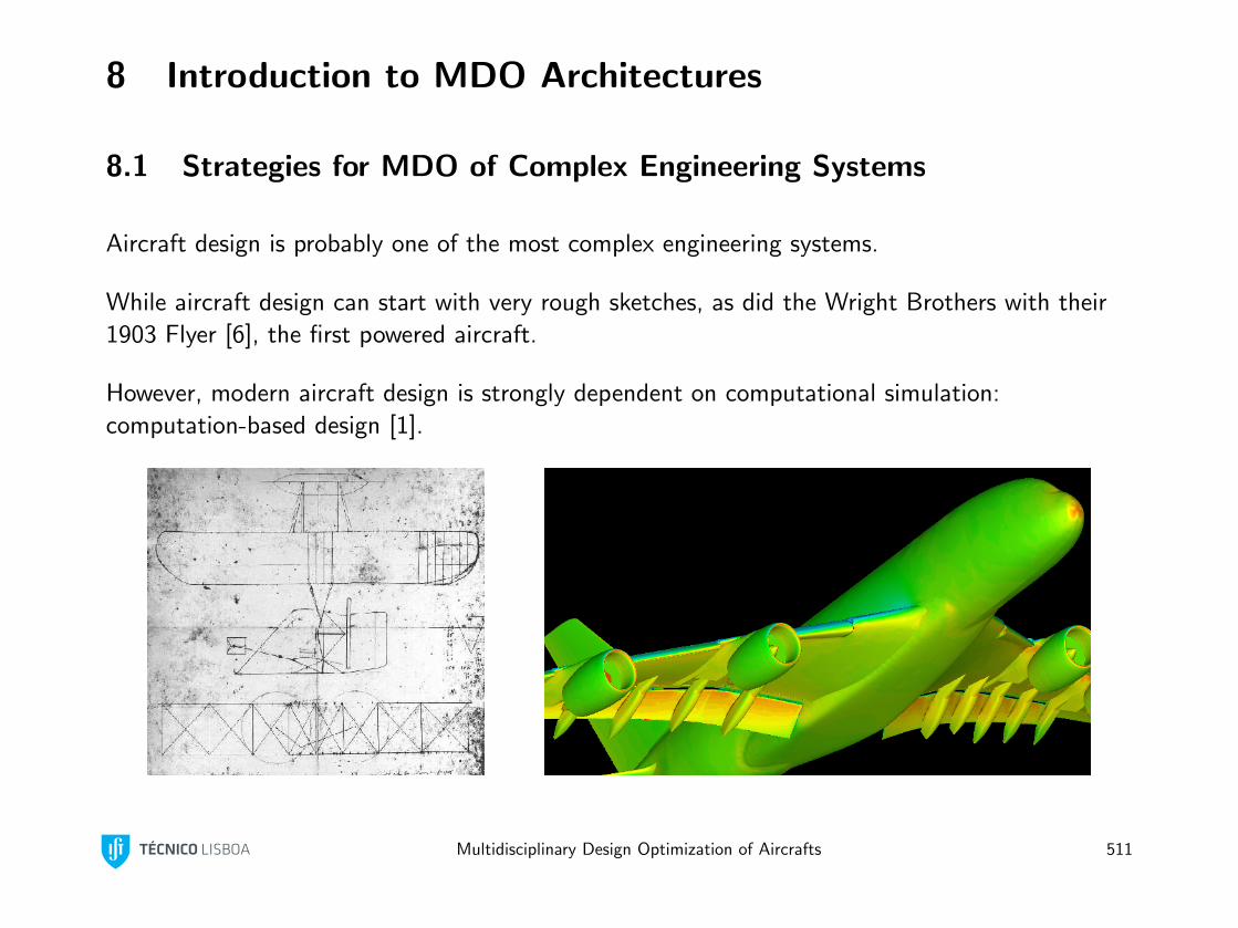
8 Introduction to MDO Architectures

8.1 Strategies for MDO of Complex Engineering Systems

Aircraft design is probably one of the most complex engineering systems.

While aircraft design can start with very rough sketches, as did the Wright Brothers with their

1903 Flyer [6], the first powered aircraft.

However, modern aircraft design is strongly dependent on computational simulation:

computation-based design [1].


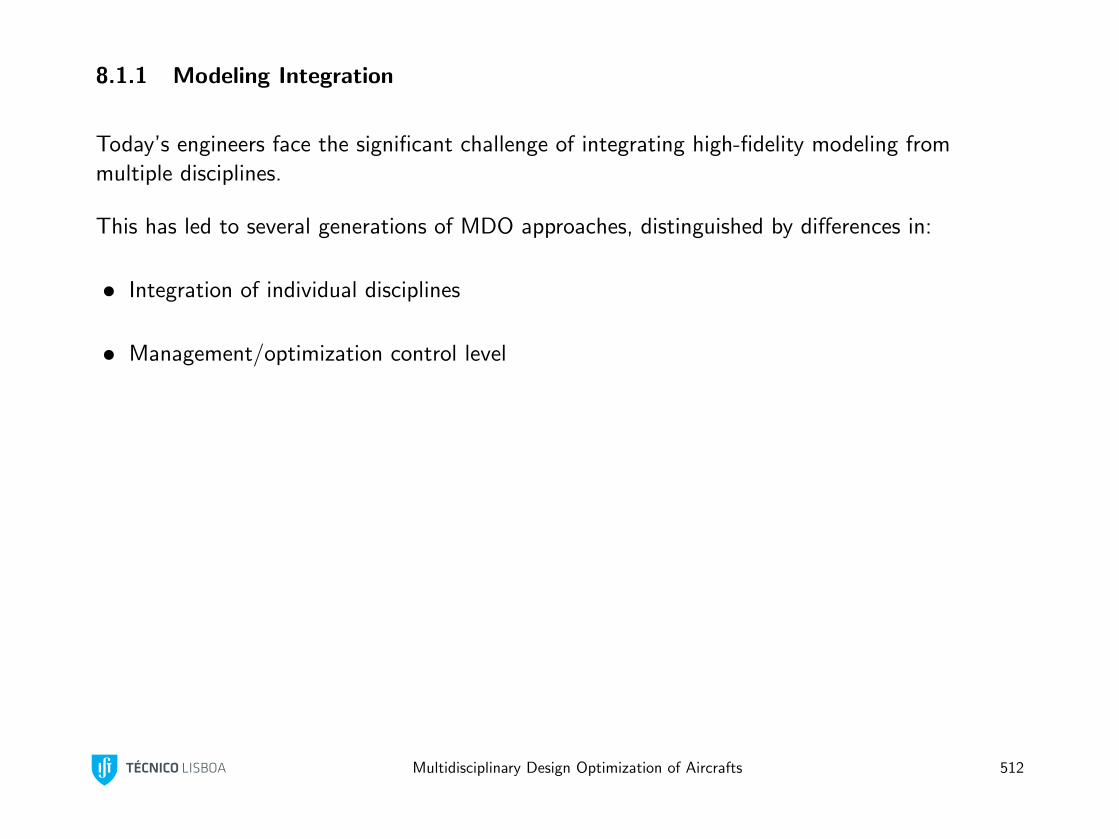
8.1.1 Modeling Integration

Today’s engineers face the significant challenge of integrating high-fidelity modeling from

multiple disciplines.

This has led to several generations of MDO approaches, distinguished by differences in:

• Integration of individual disciplines

• Management/optimization control level


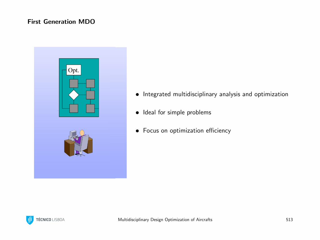
First Generation MDO

• Integrated multidisciplinary analysis and optimization

• Ideal for simple problems

• Focus on optimization efficiency


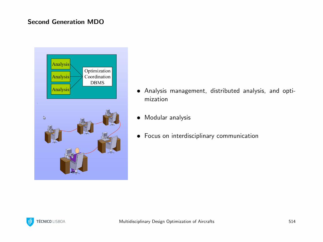
Second Generation MDO

• Analysis management, distributed analysis, and opti-

mization

• Modular analysis

• Focus on interdisciplinary communication


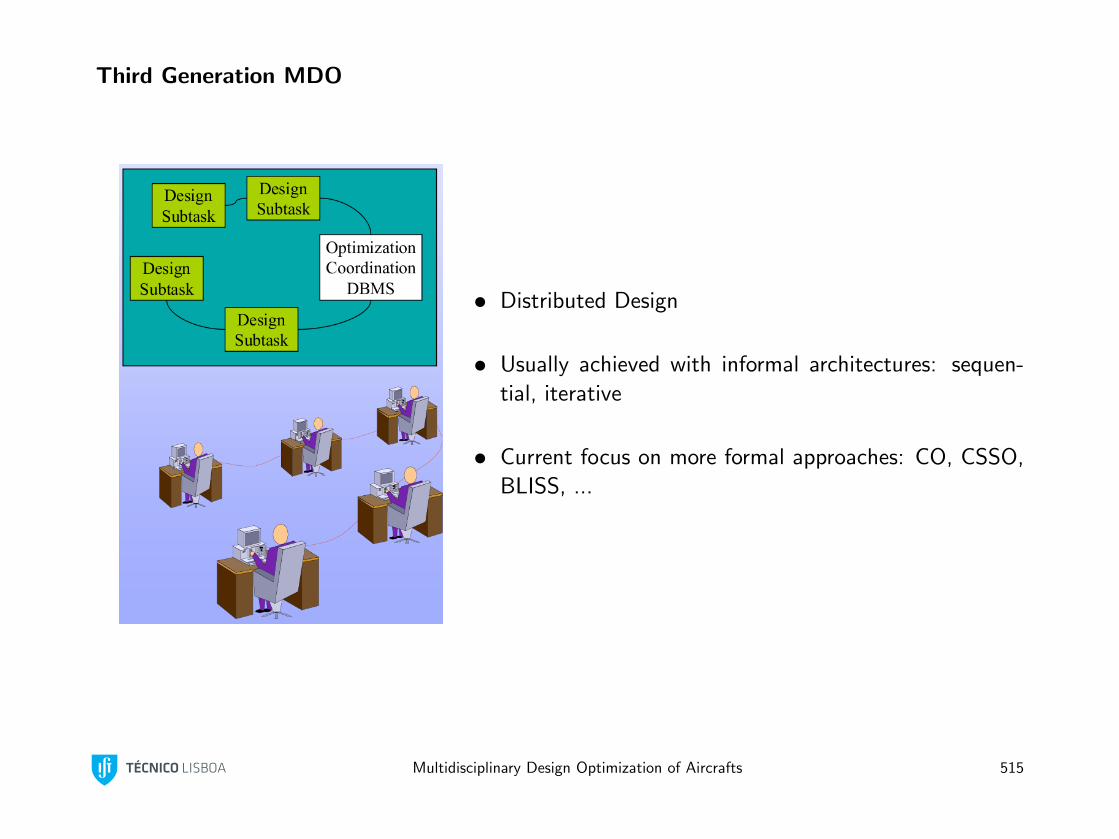
Third Generation MDO

• Distributed Design

• Usually achieved with informal architectures: sequen-

tial, iterative

• Current focus on more formal approaches: CO, CSSO,

BLISS, ...


8.1.2 Problem Decomposition

Several types of decompositions are possible when tackling an MDO problem:

• Monolithic (no decomposition)

• Decomposed analysis (OBD)

• Decomposed optimization:

– Hierarchical optimization (rare)

– Concurrent subspace optimization (one of first non-hierarchical)

– Collaborative optimization

This led to different architectures, as detailed in Sections 9 and 10.


8.2 Formal Approach to MDO

In the early 90’s, a formal approach to MDO started with the pioneer work of Sobieski [12].

Multidisciplinary design optimization (MDO) is a field of growing recognition in both academic

and industrial circles. Multidisciplinary design by itself is by no means a recent insight: the

Wright brothers realized that they needed to simultaneously consider multiple disciplines in

order to successfully design a powered airplane. Aircraft are prime examples of multidisciplinary

systems where the interaction between the different disciplines is extremely important.

In the last few decades have numerical techniques that predict the performance of engineering

systems have been developed and are now mostly mature areas of research. Numerical

optimization made use of these techniques to further automate the design process by

automatically searching the space of possible designs and by providing a mathematical definition

of what constitutes an optimum design.


While single-discipline optimization is in some cases quite mature, the design and optimization of

systems that involve more than one discipline is still in its infancy. Although there have been

hundreds of research papers written on the subject, MDO has still not lived up to its full

potential.

In the opinion of some MDO researchers, industry won’t adopt MDO because they don’t realize

their utility. Some engineers in industry think that researchers are making a big deal out of a

concept that they have always used in their work.

There is some truth to each of these perspectives. Real-world aerospace design problem may

involve thousands of variables and hundreds of analyses and engineers. This kind of problem has

so far been of a much larger scale than what has been studied by researchers.


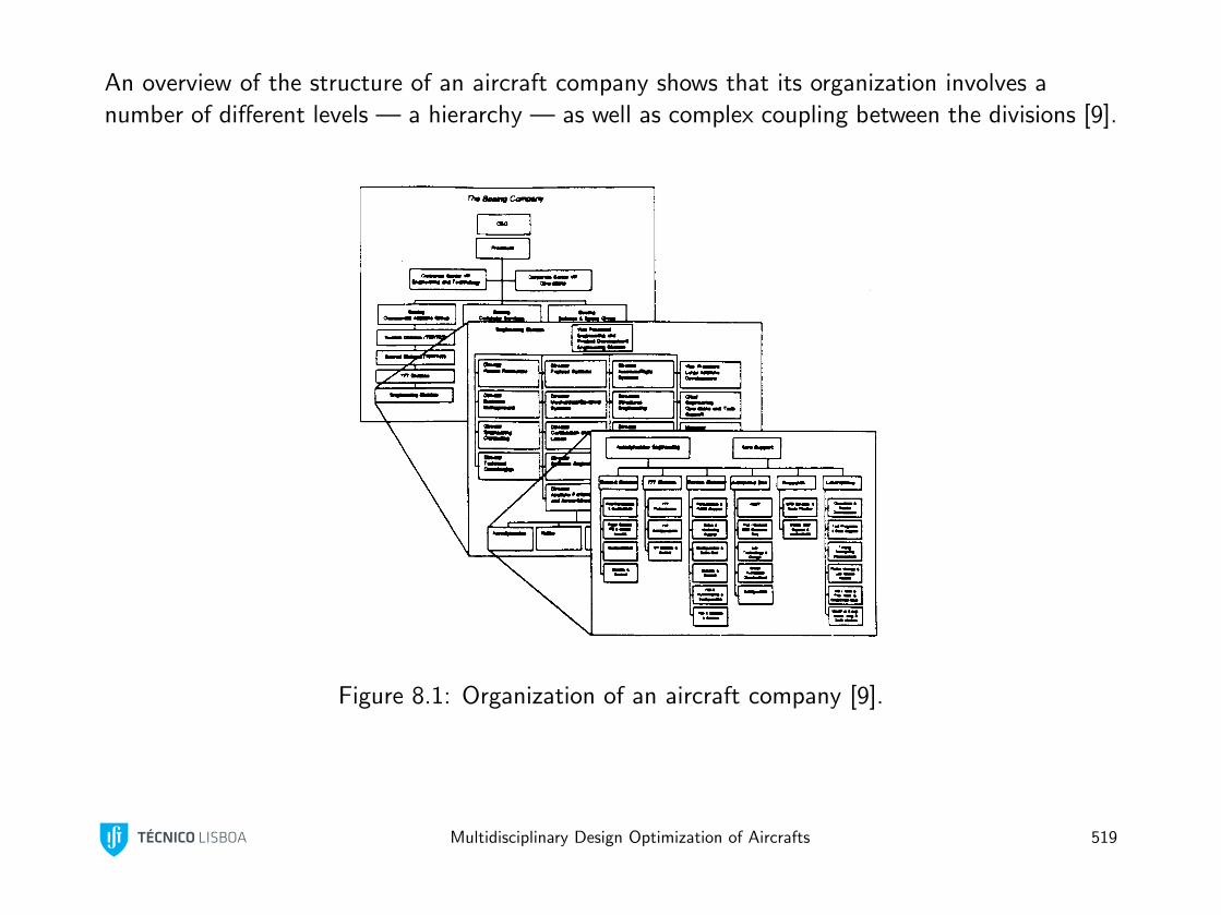
An overview of the structure of an aircraft company shows that its organization involves a

number of different levels — a hierarchy — as well as complex coupling between the divisions [9].

Figure 8.1: Organization of an aircraft company [9].


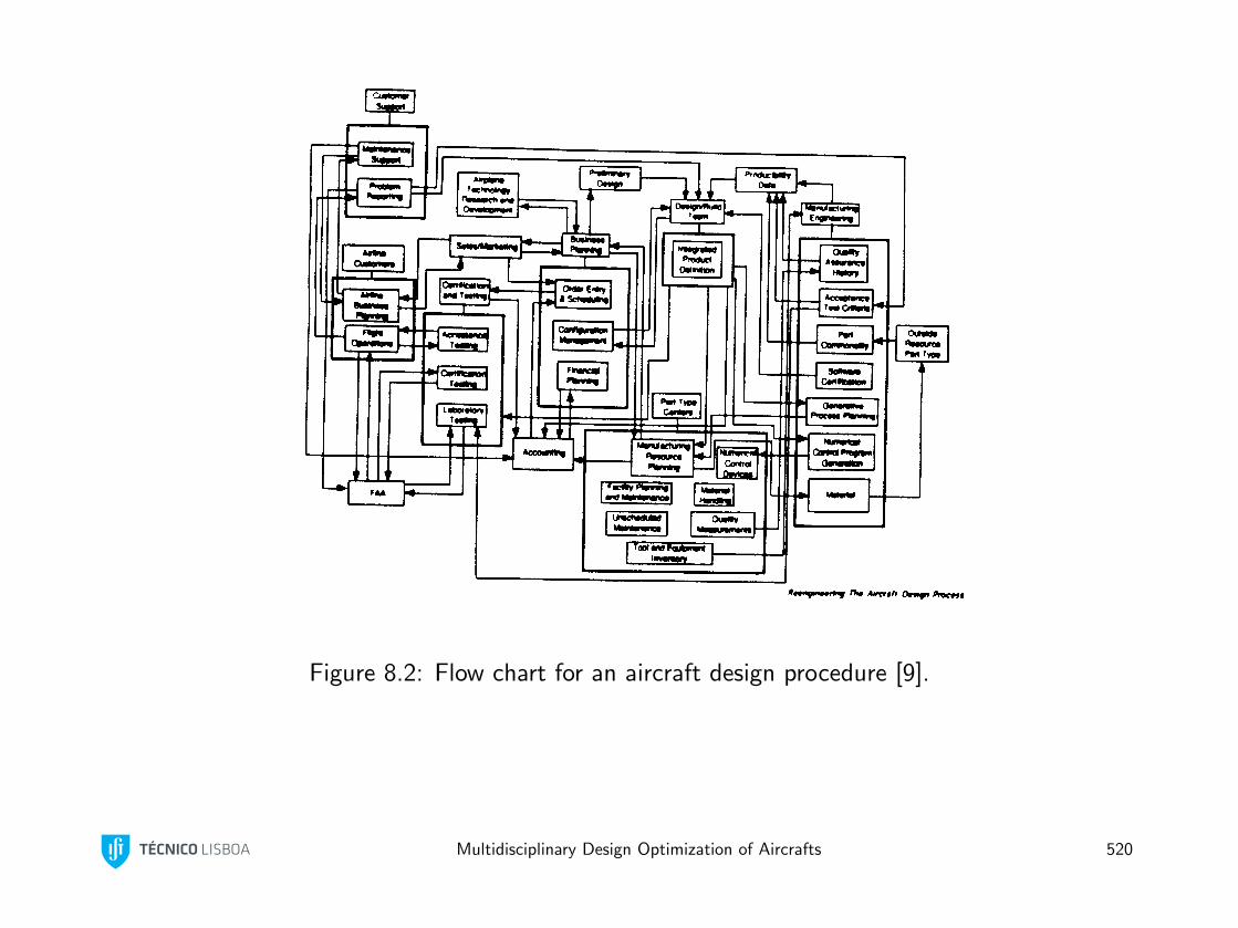
Figure 8.2: Flow chart for an aircraft design procedure [9].


Traditionally, designers have resorted to a series of parametric studies to make design decisions.

This involves plotting a figure of merit or constraint versus one or three design parameters. This

studies are limited because of the inherent difficulty of visualizing data that has more than three

dimensions. In addition, the computational cost of such studies is proportional to pn where p is

the number of points evaluated in each direction and n is the number of design variables.

MDO is concerned with the development of strategies that utilize current numerical analyses and

optimization techniques to enable the automation of the design process of a multidisciplinary

system. One of the big challenges is to make sure that such a strategy is scalable and that it will

work in realistic problems.

An MDO architecture is a particular strategy for organizing the analysis software,

optimization software, and optimization subproblem statements to achieve an optimal

design.


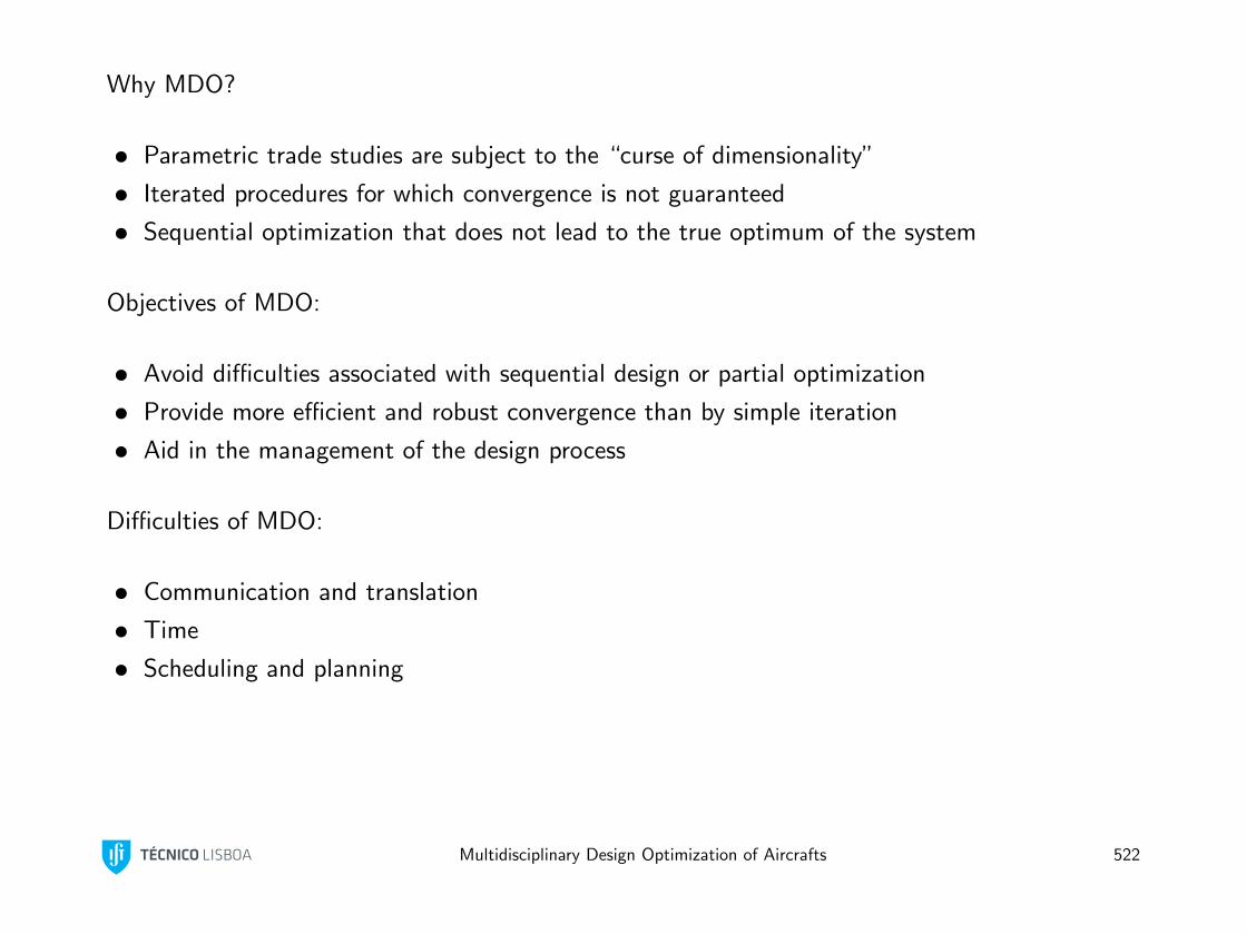
Why MDO?

• Parametric trade studies are subject to the “curse of dimensionality”

• Iterated procedures for which convergence is not guaranteed

• Sequential optimization that does not lead to the true optimum of the system

Objectives of MDO:

• Avoid difficulties associated with sequential design or partial optimization

• Provide more efficient and robust convergence than by simple iteration

• Aid in the management of the design process

Difficulties of MDO:

• Communication and translation

• Time

• Scheduling and planning


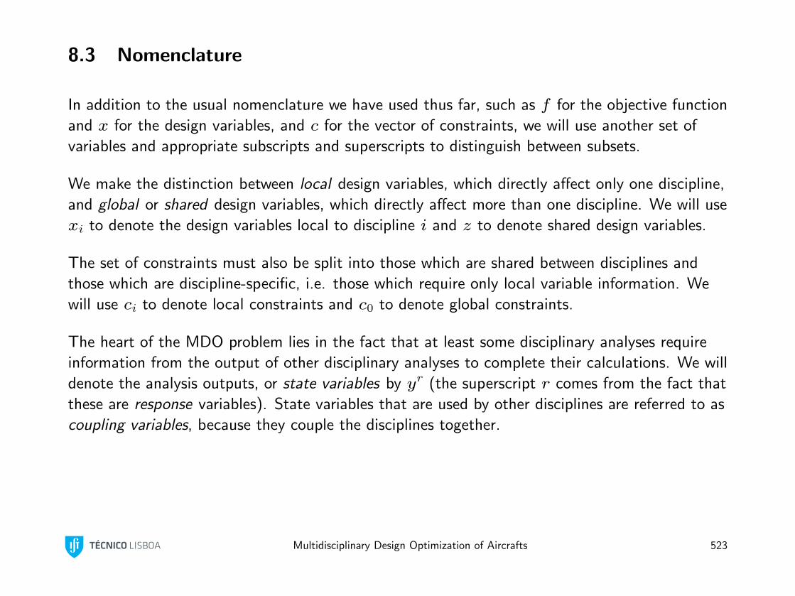
8.3 Nomenclature

In addition to the usual nomenclature we have used thus far, such as f for the objective function

and x for the design variables, and c for the vector of constraints, we will use another set of

variables and appropriate subscripts and superscripts to distinguish between subsets.

We make the distinction between local design variables, which directly affect only one discipline,

and global or shared design variables, which directly affect more than one discipline. We will use

xi to denote the design variables local to discipline i and z to denote shared design variables.

The set of constraints must also be split into those which are shared between disciplines and

those which are discipline-specific, i.e. those which require only local variable information. We

will use ci to denote local constraints and c0 to denote global constraints.

The heart of the MDO problem lies in the fact that at least some disciplinary analyses require

information from the output of other disciplinary analyses to complete their calculations. We will

denote the analysis outputs, or state variables by yr (the superscript r comes from the fact that

these are response variables). State variables that are used by other disciplines are referred to as

coupling variables, because they couple the disciplines together.


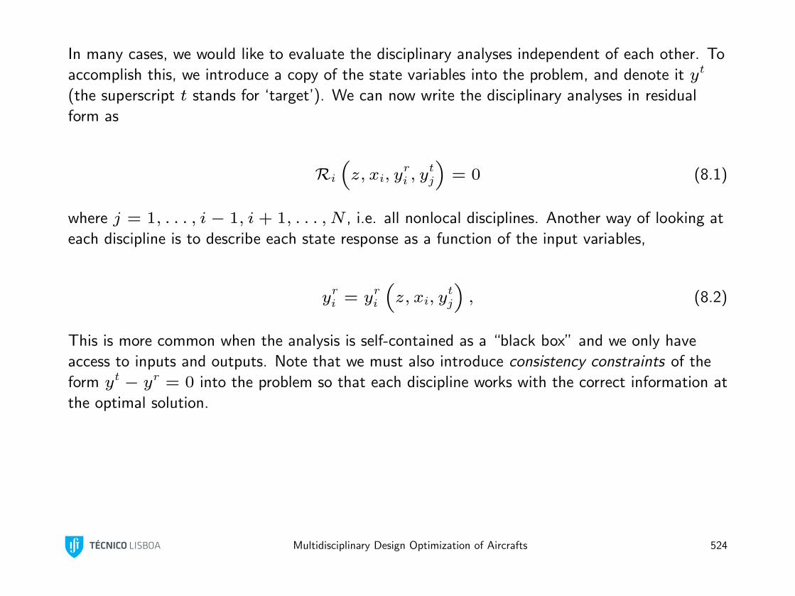
In many cases, we would like to evaluate the disciplinary analyses independent of each other. To

accomplish this, we introduce a copy of the state variables into the problem, and denote it yt

(the superscript t stands for ‘target’). We can now write the disciplinary analyses in residual

form as

Ri

(z, xi, y

ri , y

tj

)= 0 (8.1)

where j = 1, . . . , i− 1, i+ 1, . . . , N , i.e. all nonlocal disciplines. Another way of looking at

each discipline is to describe each state response as a function of the input variables,

yri = y

ri

(z, xi, y

tj

), (8.2)

This is more common when the analysis is self-contained as a “black box” and we only have

access to inputs and outputs. Note that we must also introduce consistency constraints of the

form yt − yr = 0 into the problem so that each discipline works with the correct information at

the optimal solution.


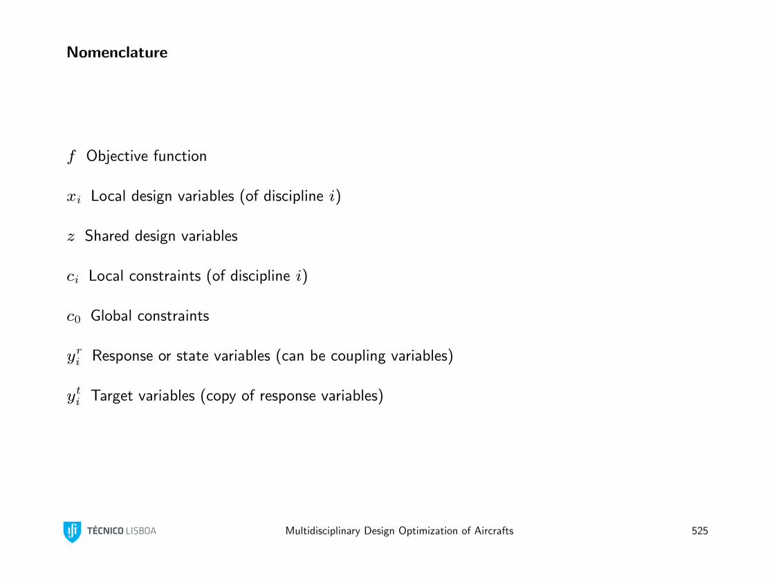
Nomenclature

f Objective function

xi Local design variables (of discipline i)

z Shared design variables

ci Local constraints (of discipline i)

c0 Global constraints

yri Response or state variables (can be coupling variables)

yti Target variables (copy of response variables)


8.4 Multidisciplinary Analysis (MDA)

If we want to know how the system behaves for a given set of design variables without

optimization, we need to repeat each disciplinary analysis until each yti = yri . This is called a

multidisciplinary analysis (MDA). There are many possible techniques for converging the MDA

but for now we will assume that the MDA is converged by a sequential (Gauss-Seidel) approach.

Discipline 1

Discipline 2

Discipline 3

y1

y2y2

y3

Figure 8.3: Example of Multidisciplinary Analysis.


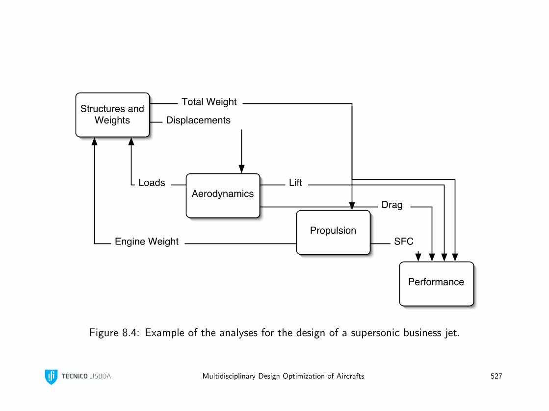
Structures and Weights

Aerodynamics

Propulsion

Performance

Displacements

Loads

Engine Weight

Total Weight

SFC

Drag

Lift

Figure 8.4: Example of the analyses for the design of a supersonic business jet.


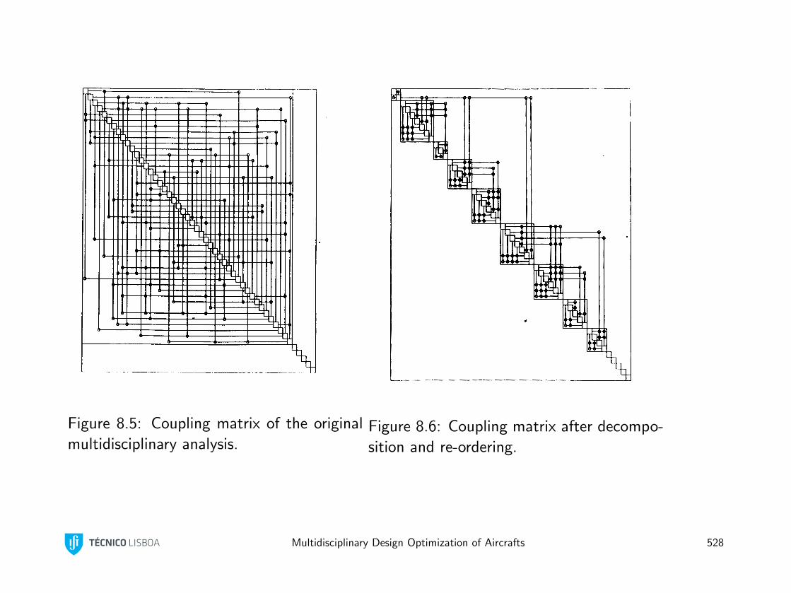
Figure 8.5: Coupling matrix of the original

multidisciplinary analysis.Figure 8.6: Coupling matrix after decompo-

sition and re-ordering.


8.5 Pitfalls of Sequential Approach

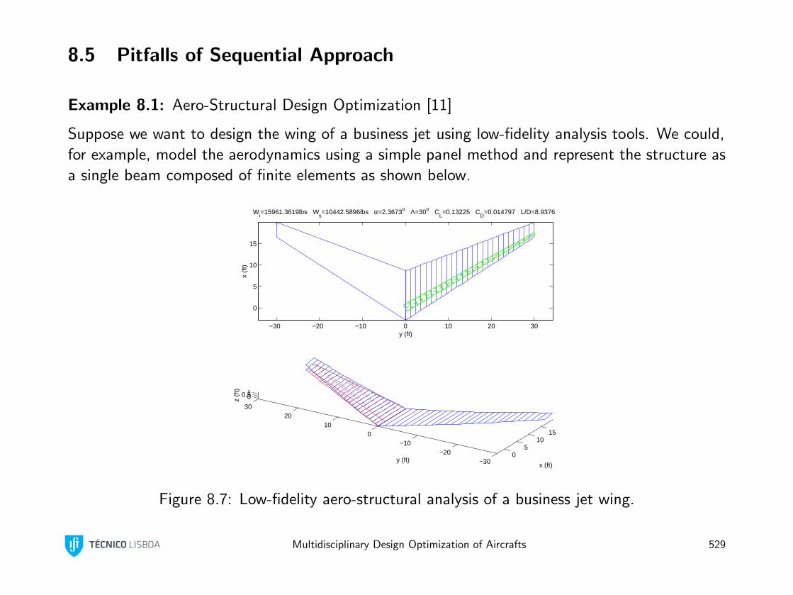
Example 8.1: Aero-Structural Design Optimization [11]

Suppose we want to design the wing of a business jet using low-fidelity analysis tools. We could,

for example, model the aerodynamics using a simple panel method and represent the structure as

a single beam composed of finite elements as shown below.

−30 −20 −10 0 10 20 30

0

5

10

15

y (ft)

x (f

t)

Wi=15961.3619lbs W

s=10442.5896lbs α=2.3673o Λ=30o C

L=0.13225 C

D=0.014797 L/D=8.9376

05

1015

−30−20

−100

1020

30

00.51

x (ft)y (ft)

z (f

t)

Figure 8.7: Low-fidelity aero-structural analysis of a business jet wing.


The panel method takes an angle-of-attack (α) a twist distribution (γi) and computes the lift

(L) and inviscid, incompressible drag (D). The structural analysis takes the thicknesses of the

beam (ti) and computes the structural weight, which is added to a fixed weight to obtain the

total weight (W ). The maximum stresses in each finite-element (σi) are also calculated.

How do we perform design using optimization?


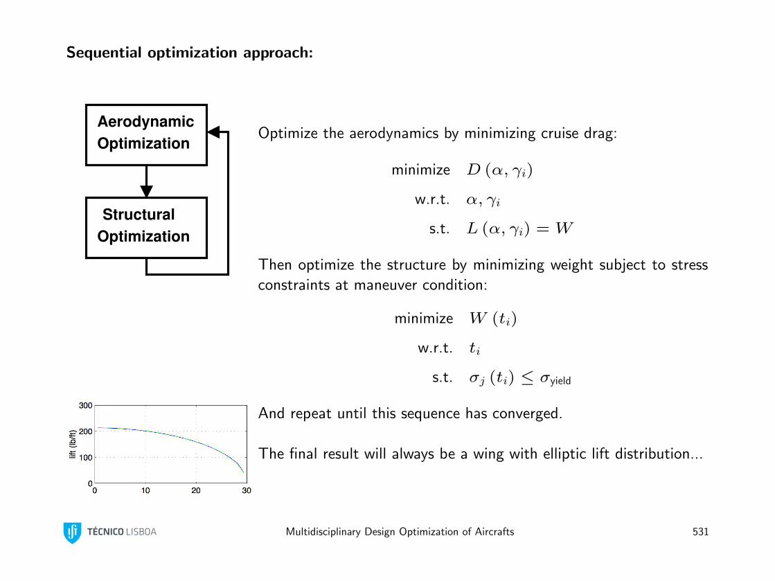
Sequential optimization approach:

OptimizationStructural

OptimizationAerodynamic

Optimize the aerodynamics by minimizing cruise drag:

minimize D (α, γi)

w.r.t. α, γi

s.t. L (α, γi) = W

Then optimize the structure by minimizing weight subject to stress

constraints at maneuver condition:

minimize W (ti)

w.r.t. ti

s.t. σj (ti) ≤ σyield

And repeat until this sequence has converged.

The final result will always be a wing with elliptic lift distribution...


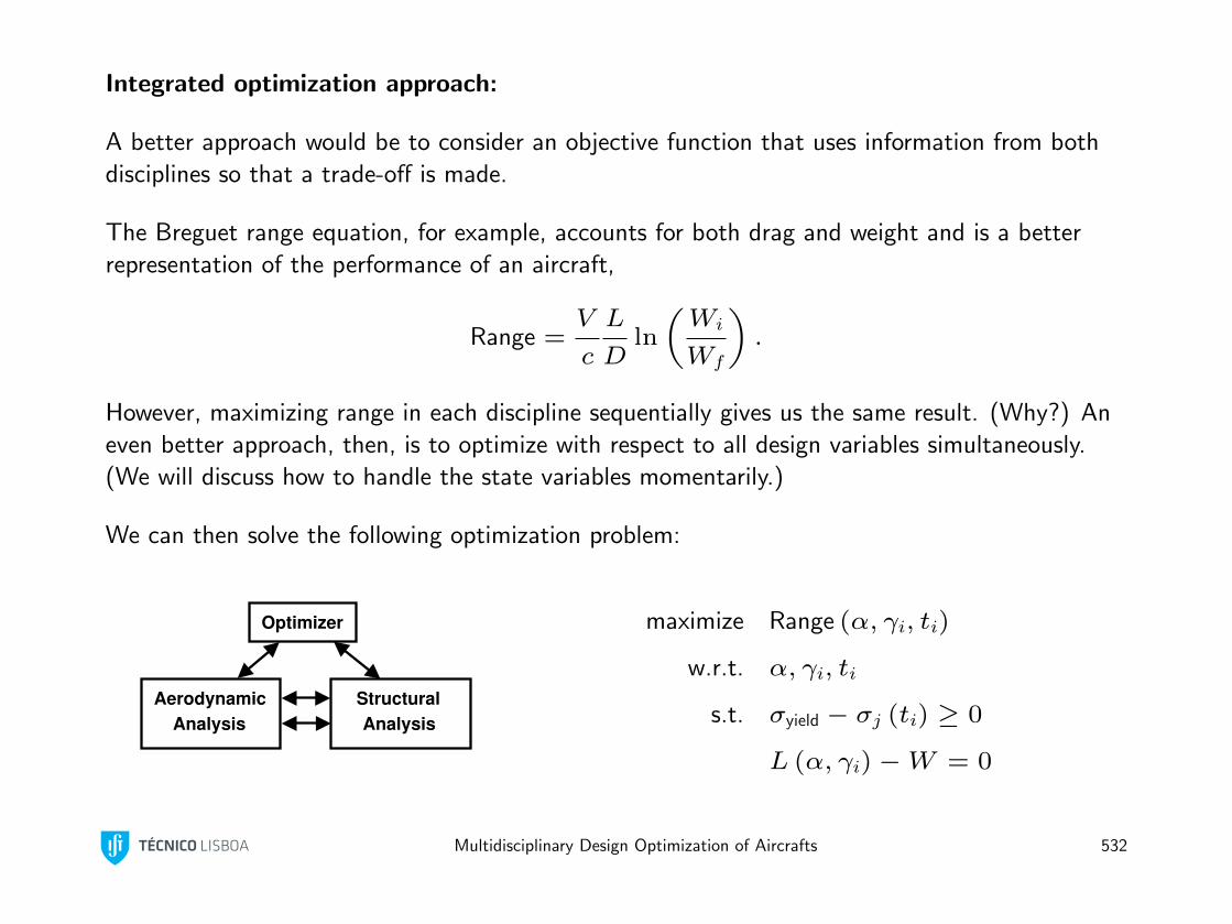
Integrated optimization approach:

A better approach would be to consider an objective function that uses information from both

disciplines so that a trade-off is made.

The Breguet range equation, for example, accounts for both drag and weight and is a better

representation of the performance of an aircraft,

Range =V

c

L

Dln

(Wi

Wf

).

However, maximizing range in each discipline sequentially gives us the same result. (Why?) An

even better approach, then, is to optimize with respect to all design variables simultaneously.

(We will discuss how to handle the state variables momentarily.)

We can then solve the following optimization problem:

Aerodynamic Analysis

Optimizer

Structural Analysis

maximize Range (α, γi, ti)

w.r.t. α, γi, ti

s.t. σyield − σj (ti) ≥ 0

L (α, γi)−W = 0


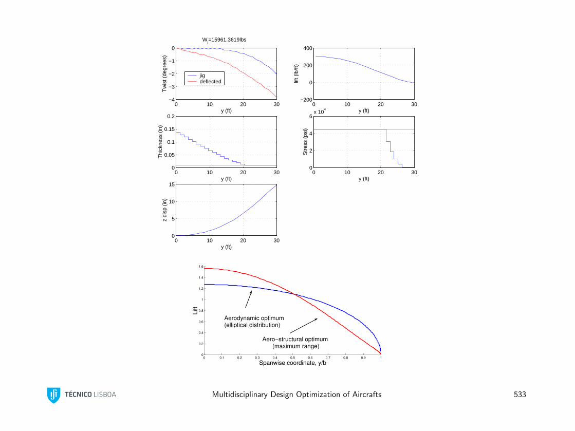
0 10 20 30−4

−3

−2

−1

0

y (ft)

Tw

ist (

degr

ees)

Wi=15961.3619lbs

jig deflected

0 10 20 30−200

0

200

400

y (ft)

lift (

lb/ft

)

0 10 20 300

0.05

0.1

0.15

0.2

y (ft)

Thi

ckne

ss (

in)

0 10 20 300

2

4

6x 10

4

y (ft)

Str

ess

(psi

)

0 10 20 300

5

10

15

y (ft)

z di

sp (

in)

0 0.1 0.2 0.3 0.4 0.5 0.6 0.7 0.8 0.9 10

0.2

0.4

0.6

0.8

1

1.2

1.4

1.6

Spanwise coordinate, y/b

Lift

Aerodynamic optimum (elliptical distribution)

Aero−structural optimum (maximum range)

Student Version of MATLAB


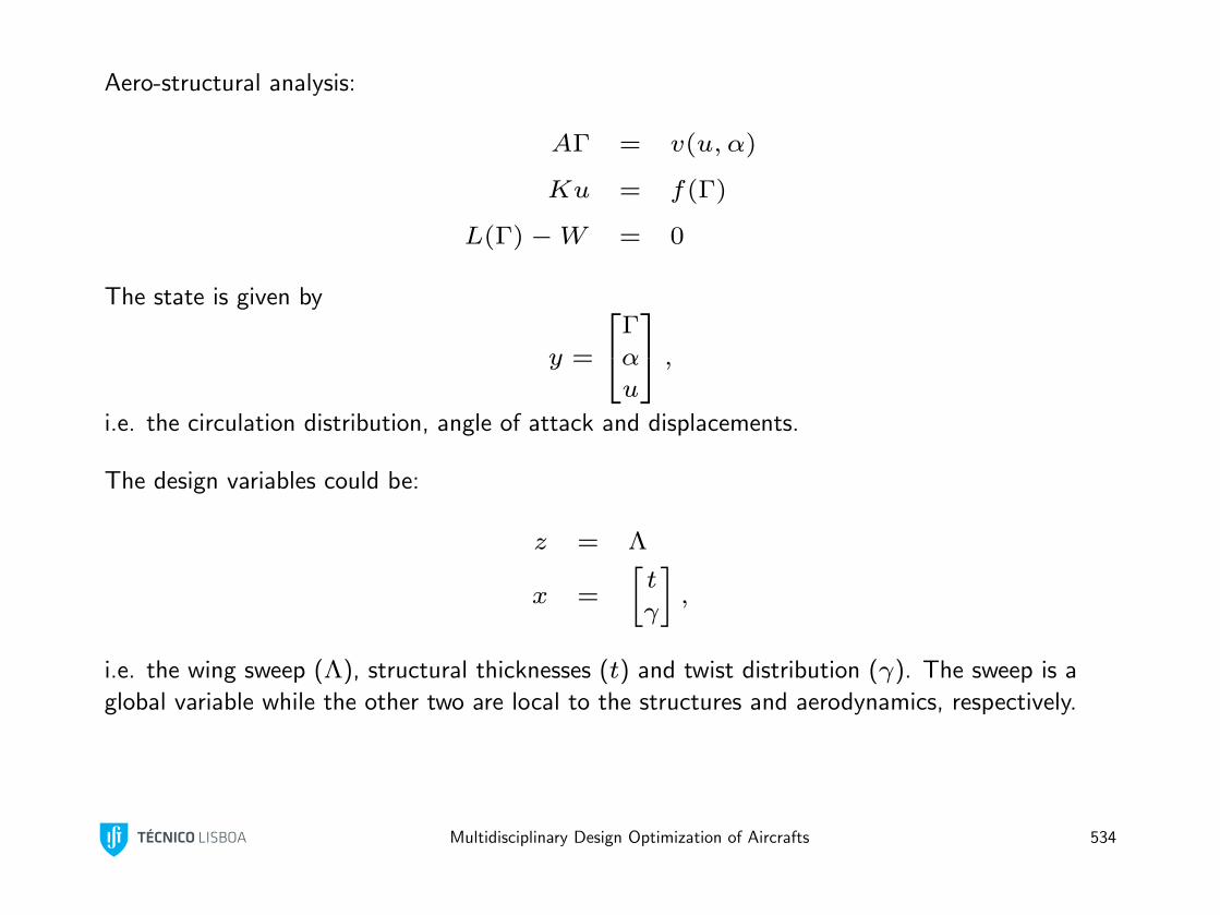
Aero-structural analysis:

AΓ = v(u, α)

Ku = f(Γ)

L(Γ)−W = 0

The state is given by

y =

Γ

α

u

,i.e. the circulation distribution, angle of attack and displacements.

The design variables could be:

z = Λ

x =

[t

γ

],

i.e. the wing sweep (Λ), structural thicknesses (t) and twist distribution (γ). The sweep is a

global variable while the other two are local to the structures and aerodynamics, respectively.


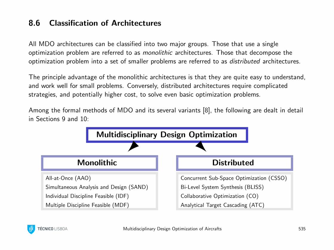
8.6 Classification of Architectures

All MDO architectures can be classified into two major groups. Those that use a single

optimization problem are referred to as monolithic architectures. Those that decompose the

optimization problem into a set of smaller problems are referred to as distributed architectures.

The principle advantage of the monolithic architectures is that they are quite easy to understand,

and work well for small problems. Conversely, distributed architectures require complicated

strategies, and potentially higher cost, to solve even basic optimization problems.

Among the formal methods of MDO and its several variants [8], the following are dealt in detail

in Sections 9 and 10:

Multidisciplinary Design Optimization

Monolithic

All-at-Once (AAO)

Simultaneous Analysis and Design (SAND)

Individual Discipline Feasible (IDF)

Multiple Discipline Feasible (MDF)

Distributed

Concurrent Sub-Space Optimization (CSSO)

Bi-Level System Synthesis (BLISS)

Collaborative Optimization (CO)

Analytical Target Cascading (ATC)


MDO techniques apply various decomposition and coordination methods to facilitate

communication between several disciplines while utilizing common optimization solvers to find a

solution.

Sub-optimization functions can be contained within the subsystems with appropriate coupling

variables linking all the systems and subsystems together to ensure a global objective is

maintained.

The classification shown previously is the most commonly accepted and is based on the different

decomposition and coordination strategies adopted. An alternative classifications of MDO

problems based on the type of variables being considered and the objective functions being

optimized can be found in reference [5].


References

[1] DLR German Aerospace Agency. Aeronautics research. http://www.dlr.de, 2012.

Accessed in February.

[2] Natalia M. Alexandrov. Multilevel methods for MDO. In N. Alexandrov and M. Y. Hussaini,

editors, Multidisciplinary Design Optimization: State-of-the-Art, pages 79–89. SIAM, 1997.

[3] Natalia M. Alexandrov and Robert Michael Lewis. Comparative properties of collaborative

optimization and other approaches to MDO. In Proceedings of the First ASMO UK /

ISSMO Conference on Engineering Design Optimization, Ilkley, UK, 1999.

NASA/CR-1999-209354.

[4] R. D. Braun and I. M. Kroo. Development and application of the collaborative optimization

architecture in a multidisciplinary design environment. In N. Alexandrov and M. Y. Hussaini,

editors, Multidisciplinary Design Optimization: State of the Art, pages 98–116. SIAM, 1997.

[5] Brad M. Brochtrup and Jeffrey W. Herrmann. A classification framework for product design

optimization. In Proceedings of the IDETC/CIE 2006, Philadelphia, Pennsylvania, USA,

September 2006. ASME International Design Engineering Technical Conferences &

Computers and Information in Engineering Conference. DETC2006-99308.

[6] Wright Brothers Aeroplane Company. Virtual museum. http://wright-brothers.org,

2012. Accessed in February.

[7] Victor DeMiguel. Two Decomposition Algorithms for Nonconvex Optimization Problems

with Global Variables. PhD thesis, Stanford University, Stanford, CA, 2001.


http://www.dlr.de

http://wright-brothers.org

[8] Srinivas Kodiyalam and Jaroslaw Sobieszczanski-Sobieski. Multidisciplinary design

optimization - some formal methods, framework requirements, and application to vehicle

design. Int. J. Vehicle Design, (Special Issue):3–22, 2001.

[9] Ilan M. Kroo. MDO for large-scale design. In N. Alexandrov and M. Y. Hussaini, editors,

Multidisciplinary Design Optimization: State-of-the-Art, pages 22–44. SIAM, 1997.

[10] Ilan M. Kroo, Steve Altus, Robert D. Braun, Peter J. Gage, and Ian P. Sobieski.

Multidisciplinary optimization methods for aircraft preliminary design. In Proceedings of the

5th AIAA/USAF/NASA/ISSMO Symposium on Multidisciplinary Analysis and

Optimization, Panama City, FL, 1994.

[11] Joaquim R. R. A. Martins. A Coupled-Adjoint Method for High-Fidelity Aero-Structural

Optimization. PhD thesis, Stanford University, Stanford, CA, 2002. Appendix A.

[12] Jaroslaw Sobieszczanski-Sobieski. Multidisciplinary design optimization: An emerging new

engineering discipline. NASA/TM 1993-107761, 1993.


7 optimization in matlab - ulisboa optimization in matlab matlab (matrix labboratory) is a numerical...

Documents