794 and atically qpti er- - johns hopkins university

794 IEEE TRANSACTIONS ON ROBOTICS AND AUTOMATION, VOL. 11, NO. 6, DECEMBER 1995

atically Qpti er-

Gregory S. Chirikjian, Member, IEEE, and Joel W. Burdick

Abstract-“Hyper-redundant” robots have a very large or infinite degree of kinematic redundancy. This paper develops new methods for determining “optimal” hyper-redundant manipulator configurations based on a continuum formulation of kinematics. This formulation uses a backbone curve model to capture the robot’s essential macroscopic geometric features. The calculus of variations is used to develop differential equations, whose solution is the optimal backbone curve shape. We show that this approach is computationally efficient on a single processor, and generates solutions in O( 1) time for an N degree- of-freedom manipulator when implemented in parallel on O( N ) processors. For this reason, it is better suited to hyper-redundant robots than other redundancy resolution methods. Furthermore, this approach is useful for many hyper-redundant mechanical morphologies which are not handled by known methods.

I. INTRODUCTION

YPER-REDUNDANT” manipulators have a very large relative degree of kinematic redundancy. These

robots are analogous in design and operation to “snakes” or “tentacles.” For example, Fig. 1 shows a photograph of a 30 degree-of-freedom robot which has been constructed by the authors and to which the theory in this paper has been applied. This paper addresses the issue of computing the inverse kinematics of such highly redundant robots. We term this problem “hyper-redundancy resolution.”

Traditionally, kinematic analysis and motion planning for redundant manipulators has relied upon a pseudo-inverse [ 171, generalized inverse [20], or extended inverse [l] of the manipulator Jacobian matrix. Some have considered schemes to find redundant manipulator trajectories which optimize joint rates or torques over a whole trajectory instead of point-to-point, e.g., [25] and 1221. Other inverse kinematics schemes have been developed based on the concept of dynamic isotropy [ 181.

The principal contribution of this paper is a new and computationally efficient method for determining the kinematically optimal configurations of hyper-redundant robots. This method has a number of advantages over other possible techniques. First, it is applicable to a wide variety of hyper-redundant robot mechanical morphologies which are not handled by known redundancy resolution techniques. For example, it is useful for devices driven by distributed actuators or constructed from

Manuscript received August 4, 1994; revised January 7, 1995. This work was supported by the National Science Foundation under Grants MSS-901779, MSS-9157843, and W-9357738, and by the Office of Naval Research Young Investigator Award N00014-92-J1920.

G. S. Chirikjian is with the Department of Mechanical Engineering, Johns Hopkins University, Baltimore, MD 21218 USA.

J. W. Burdick is with the Department of Mechanical Engineering, California Institute of Technology, Pasadena, CA 91125 USA.

E E E Log Number 9414516.

(b)

Fig. 1. Photograph of 30 DOF hyper-redundant robot

pneumatic tube bundles [23], [26], where it is difficult or impossible to define a Jacobian matrix. Second, this method generates cyclic joint trajectories for a given cyclic end- effector trajectory. Third, it is computationally efficient for a large number of degrees of freedom. We show that for computation on a serial processor, the computational burden of the method grows as O ( N ) , where N is the number of actuated joints. While competing method for configuration optimization based on a Jacobian can also have computational complexity that grows as O ( N ) (see Section 11), our method can be implemented using a very simple parallel processing scheme, and so the computational burden of this new method can be reduced to 0(1) in time if distributed over O ( N )

1042-296X/95$04.00 0 1995 E E E

CHIRIKJIAN AND BURDICK KINEMATICALLY OPTIMAL HYPER-REDUNDANT MANIPULATOR CONFIGURATIONS 195

processors. That is, the computational time can be independent of the number of degrees of freedom if O ( N ) processors are used. T h i s claim has not been made for any other redundancy resolution technique for general hyper-redundant manipulator morphologies.

The method presented here is based on a “backbone curve” that captures a hyper-redundant robot’s macroscopic geometric features. The backbone concept was introduced in previous work [SI, [ l l] , and has been used as a basis for developing obstacle avoidance [71, locomotion, and grasping [9], [12] analysis and algorithms for hyper-redundant robots. This paper uses the calculus of variations to develop necessary conditions for determining backbone curve shapes which satisfy task constraints and a user-defined optimality criterion. To illustrate the idea, we focus on a cost criterion which is a weighted measure of mechanism bending and extension. Shapes generated from other optimality criteria can be formulated analogously.

A summary of the potential uses of hyper-redundant robots and previous work by other researchers in the kinematics and design of hyper-redundant robotic systems can be found in [5] and [ll]. We list here those prior works which are most relevant to this paper. Reference [24] considers an optimal shape synthesis problem for a high degree of freedom Variable Geometry Truss (VGT). The solution in [24] is an approximate one, which can be considered a subset of the method in this paper. The work presented here is also useful for a broader class of mechanisms than VGT systems. Several authors [25], [22] have presented algorithms for the “global” (or path- wise) redundancy resolution problem. They typically use the calculus of variations or optimal control theory to find joint displacement trajectories which satisfy terminal end-effector constraints and minimize a user-defined cost function. This paper focuses on optimal manipulator conjigurations, though this method can also be used for trajectory generation. The optimal shape design of thin elastic rods which implement a desired robot wrist compliance was considered in [4]. This is analogous to finding the geometry of a “stiff‘ hyper-redundant robot which best implements a desired compliance behavior.

Section I1 reviews joint-based redundancy resolution techniques which are applicable to the problem of configuration optimization. Section I11 reviews the basic backbone curve modeling technique and the associated “fitting” procedures. Section IV develops an optimality criteria for hyper-redundant manipulator shape based on a weighted measure of backbone curve bending, twisting, and extension. Section V provides a detailed application of the technique to a VGT mechanism. Section VI compares the computational and qualitative advantages of the continuum approach versus joint-based methods. Section VI1 summarizes our conclusions.

11. JOINT-BASED CONFIGURATION OPTIMIZATION Based on our experience in building and controlling the

robot seen in Fig. 1, we believe that configuration optimization is a more useful goal than trajectory optimization for hyper- redundant robots. The reasons for this are twofold. First, one is likely to build hyper-redundant robots in a modular fashion-i.e., as a cascade of many similar or identical mechanical

modules (most practical hyper-redundant robots have NOT been constructed with serial chain topologies, as they are too weak). For example, the robot in Fig. 1 is comprised of a concatenation of 10 identical modules, where each module is a 3 degree of freedom planar parallel manipulator. In order to have reasonable strength-to-weight ratios, the actuators in these modules will often have nonnegligible restrictions on bending, extension, etc. Thus, it makes sense to insure that at each configuration, the local module kinematic and mechanical constraints are not violated. This can easily be done in an approximate way via configuration optimization. Configuration optimization algorithms can also be the basis for trajectory planning schemes, in which one insures that the robot’s configuration is optimal at each point in the trajectory. The techniques of [25] extremize a criteria which is integrated over a trajectory, not at each configuration. Second, configuration optimization schemes are cyclic in subsets of the workspace void of singularities. Cyclicity can be quite important for hyper-redundant manipulators.

For the purpose of comparison to the continuum approach presented later in this paper, we now review how one might formulate configuration optimization procedures using a framework based on discrete joint displacements and a Jacobian matrix.

Recall that redundancy resolution techniques based on the pseudo-inverse (or weighted pseudo-inverse) of the manipulator Jacobian matrix are based on the idea of constrained optimization. Let 3 denote the vector of joint displacements. The weighted pseudo-inverse solution is the joint velocity vector, 3, which minimizes the instantaneous cost function i g W i subject to the linearized end-effector kinematic constraints k~ = Je. W is an N x N symmetric positive definite weighting matrix, N is the number of mechanism actuated joints, TD E RM is the desired end-effector or task coordinates, and J is the M x N manipulator Jacobian matrix. Recall that the solution to this optimization problem is 8 = J a k D , where J a = WP1JT(JW-lJT)-l is the weighted pseudo-inverse. The computational complexity of the unweighted pseudo-inverse (W = 1) is O ( N ) when J is computed recursively (see Appendix B). The weighted pseudo- inverse requires O( N ~ ~ ~ ( ~ J ’ ) ) computations for a general symmetric weighting matrix where O( N p ) computations are required to compute the components of W-l. p depends on what matrix function is used, and whether or not W(e) is defined and inverted at each timestep, or W-’ is calculated symbolically off line. This, coupled with the fact that these computations cannot be performed completely in parallel, means that there is an undesirable rise in computation time when using the pseudo-inverse (weighted or not) as the number of joints increases even if O ( N ) processors work in parallel.

The optimal conjiguration redundancy resohtion problem can be analogously defined. The goal is to minimize a cost which is a function of configuration while also satisfying end-effector position constraints

.T

- mjng(8) subject to E ( @ = f (3) - 50 = 0 (1)

e


where g($) is the cost function, f (8) is the forward kinematic function, and I D is the desired end-effector location. This method is cyclic [2], unlike the pseudo-inverse which generally is not. For the purpose of discussion, let us assume that the configuration cost is

g(8) = 5iTwe. (2) 2

- For example, if the joint displacements are defined so that 0 = 0 is the center of the joint range, then (3) is a measure of mechanism’s deformation from the center of its joint range.

There are a number of methods by which one can computationally solve (2). One of the most popular methods is the Lagrange-Newton approach [19]. This method is based on the definition of a Lagrangian

(3) -T - L(8,X) = g(8) + x .(e)

where 7; is a vector of undetermined Lagrange multipliers. An extrema of L(8,x) extremizes g(8) subject to the constraint c(8) = 0. Numerically, local extrema are found by starting with estimates 80 and 10, and then iteratively solving the matrix equation

-

\ ,

for 68, and 6&. The matrix P ( 8 k , x k ) in (4) has the form P(8, , Ik ) = Vzg(8k) + Xz02cz(8). New best estimates of the extrema are - obtained by the update rule 8,+1 = 8 k + 6 e k

and xk+l = X I , + 6Xk. This method has the advantage that if the initial estimates are good, then convergence to a local minima is quadratic. While general configuration optimization implemented with the Lagrange-Newton method requires O ( N 2 ) computations if the above quantities are defined recursively and solved iteratively (or O ( N 3 ) computations if the ( N + M ) x ( N + M ) matrix is explicitly inverted), there are some manipulator morphologies and some choices of cost functions which permit as few as O ( N ) computations with this technique (when the joint angles are defined from an appropriate datum). In these cases P and J will have special structure.

Further, one must be able to compute second derivatives of g(8) and the manipulator Hessian matrix (i.e., second derivatives of f (e)). These computations are often extremely difficult for the nonserial topologies used in practical hyper- redundant designs. A variant on this method has been derived in a different way and was implemented as a weighted pseudo- inverse for serial chain manipulators in [15], and the method was shown to be cyclic for a particular example.

Another class of numerical methods rely on a projected gradient [19]. In this approach, from an initial estimate, 80, one would like to minimize g($) by moving in the direction of the negative gradent of g(8). However, only moves which satisfy the constraints are allowed. This procedure, which is also iterative, can be performed as follows. Let 80 be an estimate of the local minima, which is assumed to satisfy the constraints. Let Z k be an N x N matrix whose columns are a basis for the null space of J ( 8 k ) (for example, the matrix

1 - Jt($k)J(Gk)). In the first step (termed the estimator step), a better estimate of the minima is obtained by taking a step in the direction of the projection of the negative gradient onto zk:

- - o k + l , O = o k - Q:Zkvg(ek). (5)

Q: > 0 is either a small constant (typically Q 5 l), or its value can be chosen using a line search.

Since the tangent space is a poor approximation to the curved constraint surface, the estimator step will result in a configuration 8k+l,o which is not on the constraint surface. This constraint violation is fixed in the subsequent “corrector” step, whose goal is to find a S8k+l ,o such that c(ek+l,O+@k+l,O) = - s. Assume that S$k+l,o = Yk’uk, where Y I , = [Fk, ) Y k , , e - I y k N ] is a basis for the range space of JT(8k+l ,o ) . In fact, one can choose YI, = JT(8k+l,o). The undetermined coefficients Tik which minimize the estimator error to lSt order are obtained as the solution to

-

(6) - - c ( ~ ~ + I , o ) = J(Wlc+l,o)YkDk.

If we do in fact choose Y k = J’(8k) and combine the estimator and corrector steps together, then we arrive at the adaptation of the well known “pseudo-inverse with null space projection” redundancy resolution scheme [2] to configuration optimization:

8 k + i =Bt , + Jt(5, - f ($k)) - ~:ZkVg(gk). (7)

While combining the estimator and predictor steps into one step is advantageous from a computational point of view, it does lead to poorer convergence than the proper estimator- corrector scheme. This scheme has computational complexity O ( N ) when the

Jacobian is computed recursively, and the null space projection term is computed by first computing the pseudo-inverse, pedorming the multiplication JVg, and then multiplying the pseudo-inverse. Otherwise, treating the Jacobian null space basis as an N x N matrix, and projecting Vg onto this basis has computational complexity O(N2) . Either way, it is clear that these computations cannot be distributed among O ( N ) processors to achieve O( 1) time performance because many of the computations are serial or recursive in nature.

Furthermore, neither the Lagrange-Newton or pseudo- inverse with gradient projection methods for configuration optimization can be easily applied to continuous morphology hyper-redundant robots (such as those made from pneumatic tube bundles (e.g., [23] ) where it is not possible to define a Jacobian in the standard sense. The remainder of this paper is dedicated to macroscopically solving the configuration optimization problem in an entirely new way: using a continuum approach.

-

In. CONTINUUM KINEMATICS OF BACKBONE CURVES

The continuum approach to hyper-redundancy resolution is based on a two-step modeling and computation procedure:

In the first step, we assume that, regardless of the mechanical implementation (e.g., the morphologies shown in Fig. 2), the hyper-redundant robot can be modeled using a continuous

CHIRIKJIAN AND BURDICK KWEMATICALLY OPTIMAL HYPER-REDUNDANT MANIPULATOR CONFIGURATIONS 191

Qn

x - -’,Physical Robot

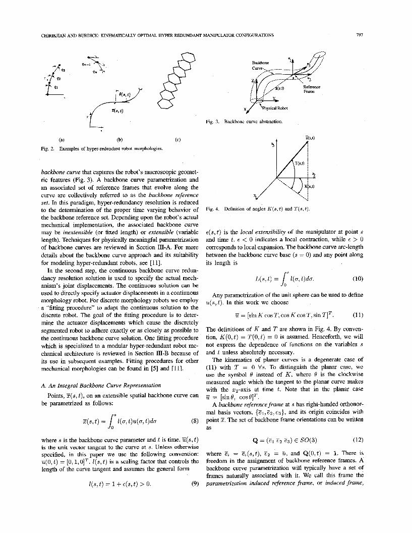
Fig. 3. Backbone curve abstraction.

(a) (b) (c)

Fig. 2. Examples of hyper-redundant robot morphologies.

backbone curve that captures the robot’s macroscopic geometric features (Fig. 3). A backbone curve parametrization and an associated set of reference frames that evolve along the curve are collectively referred to as the backbone reference set. In this paradigm, hyper-redundancy resolution is reduced to the determination of the proper time varying behavior of the backbone reference set. Depending upon the robot’s actual mechanical implementation, the associated backbone curve may be inextensible (or fixed length) or extensible (variable length). Techniques for physically meaningful parametrization of backbone curves are reviewed in Section 111-A. For more details about the backbone curve approach and its suitability for modeling hyper-redundant robots, see [ 111.

In the second step, the continuous backbone curve redundancy resolution solution is used to specify the actual mechanism’s joint displacements. The continuous solution can be used to directly specify actuator displacements in a continuous morphology robot. For discrete morphology robots we employ a “fitting procedure” to adapt the continuous solution to the discrete robot. The goal of the fitting procedure is to determine the actuator displacements which cause the discretely segmented robot to adhere exactly or as closely as possible to the continuous backbone curve solution. One fitting procedure which is specialized to a modular hyper-redundant robot mechanical architecture is reviewed in Section 111-B because of its use in subsequent examples. Fitting procedures for other mechanical morphologies can be found in [5] and 1111.

A. An Integral Backbone Curve Representation

be parametrized as follows: Points, z(s, t ) , on an extensible spatial backbone curve can

where s is the backbone curve parameter and t is time. E ( s , t ) is the unit vector tangent to the curve at s. Unless otherwise specified, in this paper we use the following convention: u(0, t ) = [0,1, OIT. Z(s, t ) is a scaling factor that controls the length of the curve tangent and assumes the general form

qs, t ) = 1 + € ( S , t ) > 0. (9)

Fig. 4. Definition of angles K ( s , t ) and T(s , t )

E ( s , ~ ) is the local extensibility of the manipulator at point s and time t . E < 0 indicates a local contraction, while E > 0 corresponds to local expansion. The backbone curve arc-length between the backbone curve base (s = 0) and any point along its length is

r s

L(s , t ) = J, Z(a, t)da

Any parametrization of the unit sphere can be used to define

(1 1)

E ( s , t ) . In this work we choose

= [sin K cos T , cos K cos T , sin TIT.

The definitions of K and T are shown in Fig. 4. By convention, K(0, t ) = T(0, t ) = 0 is assumed. Henceforth, we will not express the dependence of functions on the variables s and t unless absolutely necessary.

The kinematics of planar curves is a degenerate case of (11) with T = 0 Vs. To distinguish the planar case, we use the symbol 0 instead of K , where 0 is the clockwise measured angle which the tangent to the planar curve makes with the sz-axis at time t. Note that in the planar case U = [sinO, cosBIT.

A backbone reference frame at s has right-handed orthonormal basis vectors, {i?l,i?z,e3}, and its origin coincides with point 3. The set of backbone frame orientations can be written as

-

Q = ( E l E2 Es) E SO(3) (12)

where i?i = E%(s,t) , = ii, and Q(0, t ) = 1. There is freedom in the assignment of backbone reference frames. A backbone curve parametrization will typically have a set of frames naturally associated with it. We call this frame the parametrization induced reference frame, or induced frame,


1 The 4 x 4 homogeneous transform relating {Fi} to (Fi-1) is denoted by Hi-,. This consists of the relative translation, i and rotation, R:-l, of {Fi} with respect to {F,-l}, i.e.,

. (15) R:- (qMt ) - (qMz) ( ?iT 1

H:-,(QMa) =

qMZ E RM is the vector of joint displacements which determine the geometry of the ith module. It is assumed that the inverse kinematics of the module, which relates {F,} tb {Pi-,}, can be solved in a closed or numerically efficient form.

The manipulator configuration will exactly conform to the backbone reference set at points {s,} if

(16)

{ F ~ - I }

Fig. 5. Fitting a modular manipulator to a backbone reference set.

and denote it by QIR. For the parametrization of Fig. 4, we assign to every s the frame whose orientation is described by Hf-l(qM’(t)) = K1(sz-i , t ) X ( s , , t )

1 cos K sin K cos T - sin K sin Q I R = (-sinK cosKcosT -cosKs inT (13)

0 sin T cos T

where Q I R ( O , ~ ) = 1. The induced frame should not be confused with the backbone reference frame. It can differ from the backbone reference frame by an s-dependent twist about backbone curve tangent, which we term the roll distribution, R(s, t ) . R measures how Q twists about the backbone curve with respect to QIR, and it is defined as Q = Rot(&, R)QIR, where Rot@, 4) is rotation about axis V by angle 4 . R(0, t ) = 0 follows from the fact that Q(0, t ) = Q I R ( O , ~ ) = 1.

In summary, the backbone curve reference set, which consists of the backbone curve and associated set of orthonormal frames, is described with a small set of shupefinctions, which we denote by ?J = [K, T , R, LIT. The choice of shape function basis is not unique, and other possibilities are described in [11]. Note that the backbone reference set can also be expressed as a parametrized set of homogeneous matrices

where ?E(.) and Q(.) are defined in (8) and (12).

B. “Fitting” Procedures Here we consider a fitting procedure for a hyper-redundant

robot structure built from a concatenation of n identical modules. For example, the VGT structure of the robot in Fig. 1 fits this paradigm.

Consider the ith module (Fig. 5). Attach a frame, {F,-1}, to the “input,” or base, of the module, and a frame, {F,}, to the “output,” or top, of the module. For the discretely segmented modular manipulator configuration to conform to the continuous curve geometry, the frames {F,-l} and {F,} are chosen to coincide with the backbone reference frames at a set of n + 1 “fitting” points: {s,}. We typically choose s, = z/n for z = 0, . . . , n. Recall that equal partitioning of the curve parameter need not imply equal physical spacing along the curve, because L(.) can be chosen from a broad class of functions.

where X ( s , t ) is defined in (14). That is, the right hand side of (16) expresses the relative displacement of the backbone curve reference frame at s, with respect to the backbone curve reference frame at sz-l, while the left hand side describes the relative displacement of the ith module output frame with respect to its input frame. When the two are equated, the discrete mechanism aligns exactly with the continuous backbone curve at the n fitting points. We typically choose one of the fitting points to be the end-effector frame, so that distal position and orientation of both the continuous backbone curve and the discrete mechanism are in exact alignment. An example of this method is given in Section V.

On a serial processor, the computational burden of the fitting procedure for modular morphologies is O ( N ) . More importantly, the algorithm can easily be parallelized to great advantage. Assume that each module contains one computer processor and is connected to a central computer by a communications network. Once the backbone curve shape functions which solve a hyper-redundancy resolution problem have been computed by the central processor, each E t p l , and module inverse kinematics can be computed in parallel on the relevant processors. Thus, for modular geometries, such as the one in Fig. 1, the computational complexity of the fitting procedure is 0(1), or constant, in time for N processors. That is, it is independent of the number of modules if one chooses this simple parallel processing model and broadcast communications architecture.

W . OPTIMAL BACKBONE CURVE CONFIGURATIONS In this work we focus on “optimal” configurations that

minimize a weighted combination of bending, twisting, and local extensiodcontraction of the backbone curve while also satisfying task constraints. Using the continuous backbone curve model, this section uses the calculus of variations to compute the optimal backbone curve shapes. The optimal configurations that satisfy other criteria can be formulated in an analogous fashion.

A. Quantifying Backbone Curve Optimality Deformation of the backbone curve (and the resulting

change in hyper-redundant manipulator configuration) results

CHRIKJIAN AND BURDICK KINEMATICALLY OPTIMAL HYPER-REDUNDANT MANIPULATOR CONFIGURATIONS 199

from mechanism bending, twisting, rolling, and extensiodcontraction at each s. A dimensionally consistent cost function which includes these effects is

where t r (A) denotes the trace of matrix A, and ‘“” represents differentiation with respect to s. In the problem at hand, the cost function and constraints are functions of time, but since we are extremizing from point to point in time, the calculus of variations formulated for a single dependent variable (see Appendix A) is directly applicable. t r QWQT is a measure

positive semi-definite weighting matrix. We make the reasonable assumption that there is no preferred direction of bending, and hereafter W is restricted to the isotropic form W = a l , where 1 is the 3 x 3 identity matrix. Similarly, (i - 1)2 is a measure of a mechanism’s extension and contraction from its nominal length. Thus, a weights the relative cost of bending, twisting, and rolling, while ,B weights extensiodcontraction. In this section, the calculus of variations is used to generate backbone curve shapes which extremize (17). Other criteria can be similarly handled.

At s = 0, the backbone reference frame must coincide with the base frame. At s = 1, the backbone reference frame must correspond to the desired end-effector orientation, Q D . Thus, the boundary conditions

of mechanism bending and twisting. - s , ) is a 3 x 3 symmetric

are imposed on the Euler-Lagrange equations. The minimum bending problem can be stated as the minimization of (17) subject to the isoperimetric constraints 5 ( l , t ) = z ~ ( t ) (the desired end-effector position, where T(s , t ) takes the form of (9) with boundary conditions (18). (See Appendix A for a review of variational calculus and explanation of the above terminology).

The corresponding Lagrangian is

- pc is a vector of undetermined Lagrange multipliers arising from the isoperimetric end-effector constraint 5( 1, t) = T D ( t ) .

The only issue which needs to be resolved is how to choose the functions a(s) and P(s ) . The choice naturally depends on the particular hyper-redundant robot morphology and the intuition of the hyper-redundant robot user. In instances where the robot is constructed from a concatenation of uniform modules (such as in Fig. 1) or pneumatic tubes, these functions are independent of s, and the following analysis leads to a useful choice of the weighting functions.

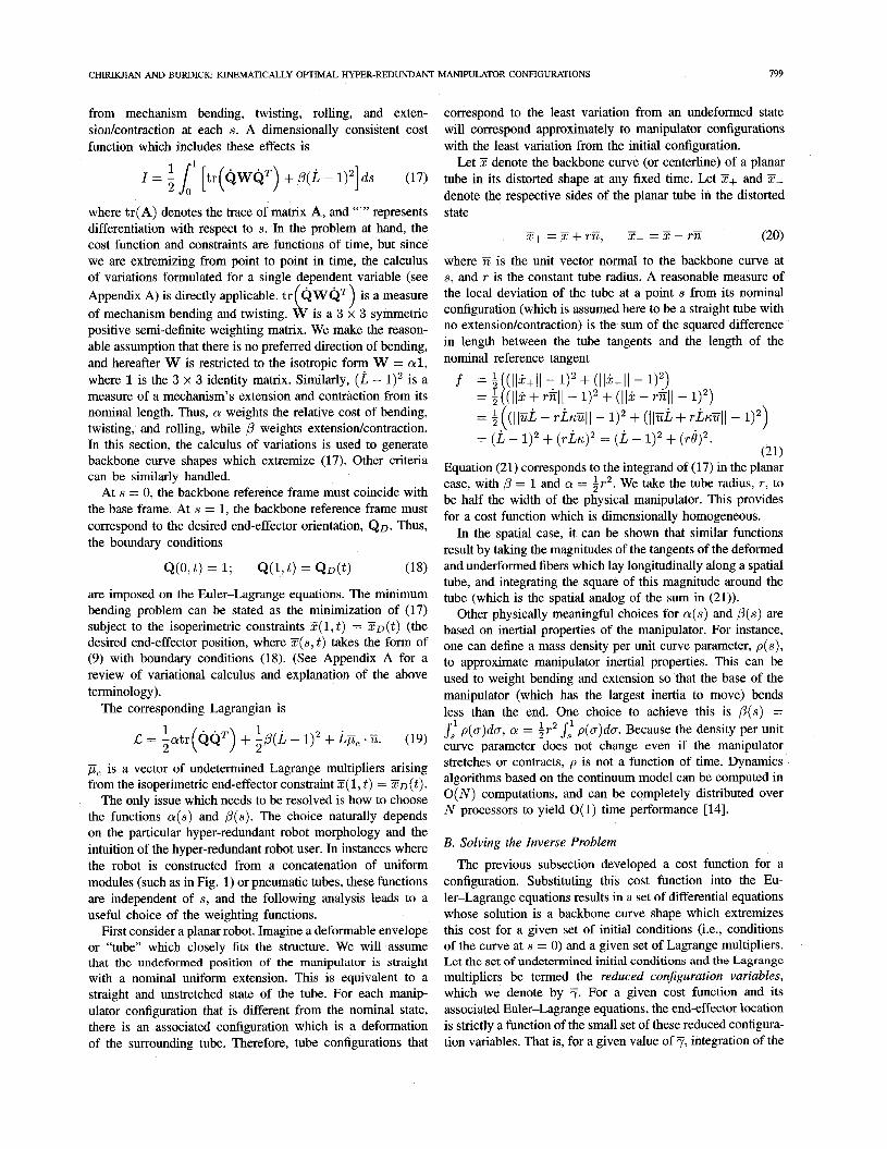
First consider a planar robot. Imagine a deformable envelope or “tube” which closely fits the structure. We will assume that the undeformed position of the manipulator is straight with a nominal uniform extension. This is equivalent to a straight and unstretched state of the tube. For each manipulator configuration that is different from the nominal state, there is an associated configuration which is a deformation of the surrounding tube. Therefore, tube configurations that

correspond to the least variation from an undeformed state will correspond approximately to manipulator configurations with the least variation from the initial configuration.

Let Z denote the backbone curve (or centerline) of a planar tube in its distorted shape at any fixed time. Let Z+ and Z- denote the respective sides of the planar tube in the distorted state

(20) x+ = 5 + r E , Z- = T - r E

where T i is the unit vector normal to the backbone curve at s, and T is the constant tube radius. A reasonable measure of the local deviation of the tube at a point s from its nominal configuration (which is assumed here to be a straight tube with no extensiodcontraction) is the sum of the squared difference in length between the tube tangents and the length of the nominal reference tangent

-

f = f((llk+ll 7 + (Ilk-11 - 1):) = f ( ( ~ ~ k + r ~ ~ ~ - ~ ) 2 + ( ~ ~ k - ~ ~ ~ ~ - l ) z )

= ( L - 1)2 + (rL6l2 = ( L - 112 + (.el2. = f (( IluL - T L m I - 1)2 + (IIuL + TLKUII - 1)2)

(21) Equation (21) corresponds to the integrand of (17) in the planar case, with /3 = 1 and a = f r 2 . We take the tube radius, r , to be half the width of the physical manipulator. This provides for a cost function which is dimensionally homogeneous.

In the spatial case, it can be shown that similar functions result by taking the magnitudes of the tangents of the deformed and underformed fibers which lay longitudinally along a spatial tube, and integrating the square of this magnitude around the tube (which is the spatial analog of the sum in (21)).

Other physically meaningful choices for a(s) and p ( s ) are based on inertial properties of the manipulator. For instance, one can define a mass density per unit curve parameter, p(s) , to approximate manipulator inertial properties. This can be used to weight bending and extension so that the base of the manipulator (which has the largest inertia to move) bends less than the end. One choice to achieve this is p ( s ) = Js’ p(a)da, a = f r 2 J, p(a)da. Because the density per unit curve parameter does not change even if the manipulator stretches or contracts, p is not a function of time. Dynamics algorithms based on the continuum model can be computed in O ( N ) computations, and can be completely distributed over N processors to yield 0 ( 1 ) time performance 1141.

1

B. Solving the Inverse Problem

The previous subsection developed a cost function for a configuration. Substituting this cost function into the Eu- ler-Lagrange equations results in a set of differential equations whose solution is a backbone curve shape which extremizes this cost for a given set of initial conditions (i.e., conditions of the curve at s = 0) and a given set of Lagrange multipliers. Let the set of undetermined initial conditions and the Lagrange multipliers be termed the reduced configuration variables, which we denote by 7. For a given cost function and its associated Euler-Lagrange equations, the end-eff ector location is strictly a function of the small set of these reduced configuration variables. That is, for a given value of 7, integration of the

800 EEE TRANSACTIONS ON ROBOTICS AND AUTOMATION, VOL. 11, NO. 6, DECEMBER 1995

Euler-Lagrange equations will produce a unique end-effector location. This section considers the “inverse” problem of determining the reduced configuration variables for a desired end-effector location. Many other techniques are known for solving this problem, as reviewed in [6]. We develop a particular method here because of its generality, because of its close resemblance to standard methods in manipulator kinematics, and for the purposes of computational complexity analysis.

Equation (S), when evaluated at s = 1, can be expressed in the general form

1

(22) - z(1,t) = 1 v(7J)ds

where ?j is the set of shape functions. If y ( s , t ) is a solution which extremizes (17) at t , subject to the constraints that z( 1, t ) = :o(t), then g is a function of t via the reduced configuration variables 7: y( s , t ) = e( s , 7( t ) ) .

The corresponding rate linearized (or “resolved rate”) kinematics commonly used in robotics can then be written symbolically as

(23) d a?? 8% -(z(l,t)) d t = [11 % s d s ] = Jz

where J is the Jacobian associated with the reduced configuration variables 7 and is termed the reduced Jacobian. Note that J is typically a 3 x 3 (4 x 4) or 6 x 6 (7 x 7) matrix for inextensible (extensible) planar or spatial backbone curves. Note that the size of J does not depend upon the number of mechanism degrees of freedom, but only on the dimension of the task coordinates (where the length of the manipulator is considered a task variable in the extensible case).

Equation (23) can be used to develop numerical procedures for solving the reduced configuration variable inverse problem. In the most simplistic approach, let To be an initial guess of the reduced variables. One can iterate the following approximation to (23) to find the values of 7 which solve the inverse problem

ayk+’ = r k + J-’(7k)Azk, (24)

where ,k is the iteration index and ATk is the error between the actual end-effector location (computed with estimated reduced variable vector 7’) and the desired end-effector location. However, to compute J(yk), one requires an expression for av(s)/a?J (which is easily obtained) and an expression for the function a%(s, ?)/ay, where $(s,7) extremizes (17). Unfor- tunately, the extremal value of 8$( s ,T) /87 can generally be realized only in numerical, and not symbolic form. We must therefore develop indirect methods for computing the extremal value of 85/87, and hence J.

The Euler-Lagrange equations will generally be of the form

(25) - 5 + f ( $ , g, 7, s) = 0

m o , 71, a o , Y), 7) = 0,

with initial conditions -

(26)

where /, f ( . ) E I R p , 7 E EL”, and f(.) E We have dropped the “hat” from $, but there is no ambiguity because

of the context in which jj is being used. P is the number of shape functions needed to fully specify the hyper-redundant- manipulator configuration, and recall that M is the number of end-effector or task coordinates. In the plane P = 2 and M is typically 3 for nonextensible robots, or M = 4 for extensible robots. For spatial manipulators P = 4 and M = 6 or 7.

Given (25) and (26), one can determine a?J/ay by a system of auxiliary differential equations. These M sets of auxiliary equations are derived by taking the derivatives of (25) and (26) with respect to the M components of 7. Since derivatives of smooth functions commute, the auxiliary equations can be expressed as the P x M matrix equation:

(27)

Note the linearity of the above equations in the auxiliary variables dy,/8y, for (2,j) E ( l , . . . , P ) x ( l , . . . ,M) . This linearity simplifies the numerical solution. The initial conditions of the 2nd order auxiliary equations are written symbolically as the 2P x M matrix equation

which can generally be separated. In addition to the com- mutation of derivatives, we have also made use of the fact that differentiation and function evaluation commute in the following cases:

Thus the extremal value of 87j/a? can be computed numerically from the auxiliary equations, and subsequently used to compute the reduced Jacobian in (23). The simultaneous (possibly parallel) solution of the original system of equations and the auxiliary equations provide the means by which the instantaneous end-effector kinematics of the hyper-redundant manipulator backbone curve is computed at each time step. If the algorithm is parallelized over M + 1 processors, the required computation time will be no greater than that of the original set of Euler-Lagrange equations plus the time required to invert the reduced Jacobian matrix.

V. A DETAILED EXAMPLE: THE OPTIMAL

A detailed application of this approach to a variable geometry truss (VGT) manipulator having the same geometry as the robot in Fig. 1 is developed in this section. The next section compares the computational complexity of this method to the noncontinuum approaches of Section I1 for the same VGT robot geometry.

In the planar case, Q consists of a rotation, by angle 8, about the axis normal to the plane. Thus,

BACKBONE CURVE FOR A PLANAR VGT

l 1 2

2 0 = - 1 [aa 8 2 + p ( L - 1) ] ds.

CHIRIKJIAN AND BURDICK KINEMATICALLY OPTIMAL. HYPER-REDUNDANT MANIPULATOR CONFIGURATIONS 801

In the case of (Y = and p = 0 (i.e., an inextensible backbone curve), this cost function becomes the integral of squared curvature. This is a problem which has been considered in detail in the mathematics, mechanics, and computer science literature [21]. Solutions for this case in terms of Elliptic functions are known.

In the extensible case, the following choice is made for hyper-redundant manipulators with homogeneous structure: a ( s ) = i r2 and p(s) = 1 (consistent with the arguments of Section IV-A). The Euler-Lagrange equations corresponding to the functions 6 and L are, respectively,

r2e - p1Lcosd + p2Lsin6 = 0 (31)

d . - (L - 1 + p1sin6 + p 2 c 0 ~ 6 ) = 0, ds

where p1 and p2 are the undetermined Lagrange multipliers associated with the planar end-effector position constraint.

We must now determine the boundary conditions and the reduced configuration variables. There are generally four task coordinates for a planar robot: x,,, yee, de,, and Lee. That is, in addition to the end-effector position and orientation, the total manipulator length from base to end-effector is also treated as a task variable. Let us consider the problem of extremizing the integral in (30) while letting O(1,t) and L(1,t) be free. That is, we do not care about the end-effector orientation or the total length of the robot in the optimal configuration. Thus the free boundary conditions ((51) in Appendix A) are used:

e(1) = 0 (33)

h( 1) - 1 + p1 sin d( 1) + p2 cos d ( 1) = 0. (34)

The initial conditions O(0) = 0 and L(0) = 0 are imposed by the fixed base conditions. The undetermined initial conditions are 8(0) and L(0). Thus, the reduced configuration variables consist of the two Lagrange multipliers and the two unspecified base boundary conditions:

These reduced configuration variables map to the four task variables through the Euler-Lagrange equations.

The solution proceeds as follows. Equation (32) has the exact first integral:

(36) L + 71 sin6 + 72cos6 = 7 4 + 72.

L from this equation can then be substituted into (31), effec- tively decoupling the 6-variable Euler-Lagrange equation from L-variable Euler-Lagrange equation. Integrating Equation (3 1) with respect to s, while observing the boundary conditions at s = 0 and (33), yields

(37)

Observing that (34) and (36) must hold simultaneously, we obtain the relation

2 --T 73 = 7lYee - 72Xee.

7 4 = 1-72. (38)

Thus, 7 4 can be eliminated, and 73 is represented in a way that directly describes its influence on end-effector position (as opposed to slope at the base of the manipulator).

In this example, there are three sets of auxiliary equations corresponding to the remaining three reduced configuration variables (since 7 4 was eliminated). Each of these sets of equations consists of two separate equations of the form

+ &2L sin 6 + 7 2 sin 6) = 0, (39) 872

86 8%

+ Si2 cos 6 - 72- sin 6 = 0, (40)

with initial conditions

for i = 1,2,3. &j = 1 when i = j and zero otherwise. Equations (39) and (40) are solved to find dO/ayi and dL/dy, .

The Jacobian matrix for this example is a 3 x 3 matrix, since one of the reduced configuration variables was eliminated. The first two rows have components

d7i 1 -(1)=1 8x1 [ ~ s i n 6 + ( l + r ) - c o s 6 d€ ds (42) d7i

872 1 $=l [Gcos6- ( l+c ) - s in6 d€ ds (43)

for i = 1,2,3. Recall that E is the extensibility: L = 1 = 1 + E.

The last row in the Jacobian matrix comes from differenti- ating (37) with respect to time, yielding

(44) dxee dye, d7l d72 2d73

r d t 72- dt - 71- dt = yee- dt - X e e z -

and so the last row in the Jacobian matrix is [yee, -xee, r2]. Having calculated the reduced Jacobian, (24) is used to find the inverse solution. The initial values of the reduced variables are 7 = 0, which corresponds to the underformed reference state 6(s,O) = 0, L(s,O) = s.

Until this point, not a single joint-based computation has been performed. In order to “algorithmically link” the backbone curve model with an actual physical device, we apply a fitting procedure to determine the discrete joint angles which cause the mechanism to exactly or closely adhere to the continuous backbone curve shape. The VGT mechanism is a modular structure, and therefore the fitting paradigm of Section 111-B can be applied. All that is required is the inverse kinematics of a VGT module, which is easily solved.

For example, Fig. 6 shows one module of the planar variable geometry truss manipulator (which is the same geometry as the robot in Fig. 1 and is described in detail in [lo]). The three

802 JEEE TRANSACTIONS ON ROBOTICS AND AUTOMATION, VOL. 11, NO. 6, DECEMBER 1995

J- jfh .\'. c k9

i - 1st face

Fig. 6. Planar variable geometry tmss fitting geometry.

vectors which are collinear with the prismatic actuators can be determined as follows:

a wUI --i - pi-l - E'.-1 + ROT(-ijJ3,6'b)5"; - 2 - c -jJtWl -Fi2-1 +ROT(-Es,QL)G i = 1 , 3 , 5 , . . -

j = 1 , 2 -1

= pi-, - E;-' + ROT( -E3, 6'L)S; i = 2,4,6, . . . (45)

where dL = Q ( s i ) - Q(si-1) and $ are the vectors to the jth vertex of the ith platform in the frame affixed to that platform. For this example, % = [-wi/2,OIT and $ = [wi/2,OIT, where wi is the width of each horizontal truss module face (Fig. 6). The controlled degrees of freedom are the lengths

49 = l l ~ l l for i = 1, . . . , n, and j = 1,2. Equations (45) and (46) provide the inverse kinematics solution for this module geometry. This procedure is used in Section VI to generate optimal configurations for a given end-effector trajectory.

VI. A COMPARISON OF THE CONTINUUM AND JOINT-BASED APPROACHES

In this section we consider the qualitative and quantitative features of the continuum approach for configuration optimization versus joint-based configuration optimization methods. We also compare the two approaches in terms of numerical efficiency for a VGT manipulator. Section VI-A discusses the applicability and computational burden of both methods. Section VI-B provides the results of numerical trials.

A. Generality and Order of Computation

Practical hyper-redundant robots have not and wilE not be constructed of a serial chain of rigid links and motors, since such designs are too weak. Consequently, most of the hyper-redundant structures built to date use nonserial structural designs and actuation schemes, such as tendons, pneumatic hoses, or seriallparallel mechanisms like the VGT. It is often difficult or impossible to define a Jacobian matrix for many of these structures. One particular example of this is the case of hyper-redundant manipulators composed of a cascade of modules where each module does not have closed form forward kinematics-as is often the case for parallel manipulators with revolute joints. In this case, the joint-based approaches of Section I1 cannot even be applied directly.

However, it is always possible to relate actuator displacements to a backbone curve (since the inverse Enematics of all kinematically sufficient serial and parallel manipulators can be performed efficiently), thereby establishing a fitting procedure. With a fitting procedure, the continuum approach is then applicable.

Moreover, the continuum approach has computational advantages over the discrete methods of Section I1 for general manipulator structures as the number of joints becomes large if sufficiently parallel computer architectures are used. Recall that the computation of the optimal shape using the continuum approach is a two phase process. First, the optimal continuous backbone curve shape is computed. The computational cost of this step is independent of the number of mechanical degrees of freedom of the actual discrete mechanism, and is therefore O(1). Next, the mechanism is "fitted" to the resulting curve. For modular designs, such as the one in Fig. 1, tlus process has a computational burden of O ( N ) when implemented on a serial processor, or O( 1) when implemented with a simple parallel computing architecture with one processor per module (or even one processor for every m modules for some number m > 1 which is independent of N) . Thus, the total computational burden of this approach scales as O ( N ) on a serial processor, or is O( 1) in time on a simple parallel processing architecture with O ( N ) processors.

Alternatively, all of the discrete joint based procedures for performing configuration optimization are at best O ( N ) in complexity when implemented on a serial processor, and some are much worse for arbitrary macroscopically serial manipulator morphologies, e.g., the Lagrange-Newton method. However, as the number of degrees of freedom increases, the continuum based approach becomes more computationally attractive for all morphologies if it and competing methods are implemented in parallel on O ( N ) processors. This is because the computations required for the continuum approach completely decouple, whereas the O( N ) computations of competing approaches do not.

One can also reduce the scaling of the computational burden of discrete approaches by going to parallel architectures. However, the architecture required for parallel computation of the Jacobian pseudo-inverse and other matridvector manipulations of conventional redundancy resolution cannot achieve O(1) time performance with O ( N ) processors. This is true in part because to achieve O ( N ) performance for the gradient projection method applied to a general manipulator morphology, the Jacobian must be computed by recursion. This does not parallelize completely, as is also the case for the matrix vector multiplications required to compute the pseudo- inverse once the Jacobian has been computed. In addition, such parallelization will require very complicated interprocessor communication and synchronization. Conversely, the parallel computing scheme for the continuum approach is trivial.

Thus, the continuum approach is favored for large num- bers of degrees of freedom. To make this comparison more concrete, we now apply the projected gradient method of Section 11 to configuration optimization of a planar VGT truss manipulator, and compare the computation time with that of the continuum approach-both running on a single processor.

CHIRIKJIAN AND BURDICK KINEMATICALLY OPTIMAL HYPER-REDUNDANT MANIPULATOR CONFIGURATIONS 803

Fig. 7. Continuum method (calculus of variations) solution.

B. Numerical Comparison of Two Approaches

In this section, we compare the computation required to determine the optimal configurations for the VGT manipulator described previously. In this numerical comparison, the end- effector of the VGT mechanism follows the straight line trajectory

with no prescribed orientation. This trajectory is approximated by 101 discrete points, i.e., Tee(t) is evaluated at intervals of At = 0.005. For configuration optimization, the goal is to determine the optimal configuration at each point along the trajectory.

We define the optimal configuration as the one which requires the least deformation, or joint displacement, from a reference configuration. In this case, the reference configuration at t = 0 corresponds to a VGT configuration in which the outside actuators have length q3,(0) = q3,+2(0) = t and the diagonal actuators have length q3%+1(O) = e. That is, the reference configuration is straight, with no extension or contraction. The vector e = Q - Q(0) measures the amount of joint displacement from the reference configuration. Note that the desired trajectory was chosen so that the manipulator is initially in its reference configuration at t = 0.

For the sake of comparison, we use two redundancy resolution methods on the trial trajectory: 1) the continuum approach with the minimum deformation criteria discussed earlier and 2) joint-based configuration optimization with the square of the norm of joint displacements as the optimization criteria implemented via gradient projection onto the Jacobian null space. The latter is implemented in two ways: Jacobian calculated numerically column by column (using the standard centered difference approximation for derivatives applied to the forward kinematic function), and the Jacobian calculated recursively. The forward kinematics for the VGT described earlier and used here can be found in [ 131. The Lagrange-Newton method is not used in this comparison, because it is generally far slower than the Jacobian-based approaches.

Our implementation of the continuum approach follows directly the developments in Section V. The weighting factors on mechanism bending in the cost function of (17) are is chosen to be B ( s ) = 1 and a(.) = r2/2, where r = & because the width of each fixed truss element is taken to be w = t, and r = w/2. The backbone curve configuration that corresponds to the undeformed reference configuration can be found by taking ~ ~ ( 0 ) = 0 in (35) for i = 1 ,2 ,3 and integrating (31) and (32). The resulting backbone curve is a

Fig. 8. Joint-based configuration optimization.

uniformly parame~zed straight line described by the shape functions 6(s,O) = 0 and L(s,O) = s. The reduced Jacobian elements are calculated at each time step using Liebnitz’s rule and Euler integration. For purposes of numerical integration with respect to s, the backbone curve interval s E [0 ,1] is subdivided into 5n intervals so that the backbone curve interval s E [s,-~,s,], which defines the motion of the ith module, is approximated by five segments. The configurations resulting from this method are shown in Fig. 7 for a 10 module VGT mechanism (with the same topology as the robot in Fig. 1). The configurations are shown at intervals of At = 0.1 starting at t = 0.1.

The joint-based configuration optimization simulation uses the projected gradient method reviewed in Section 11. The objective function is

1 - - 2

g(3) = -6.6,

where 3 is the displacement of the joints from their reference configuration position. We have taken a = 3m < 1, so the influence of the null space term becomes more pronounced the further the configuration is from the global minimum of the cost function. If one were to do a line search for the optimal value of Q (which would be the most rigorous approach) this would add to the computational requirements of this method.

Unlike the continuum approach, the joint-based approach requires us to compute the derivatives of the VGT forward kinematics equations. Since we are comparing this method for VGT structures consisting of 2 to 20 modules, it would be too tedious to derive closed form algebraic expressions for all the derivatives. In fact, the need to derive expressions for these derivatives for the parallelherial structures often used in real hyper-redundant systems is a major drawback of the Jacobian based methods. Instead, we numerically evaluate derivatives for each module and recursively compute the Jacobian as outlined in Appendix B.

The configurations resulting from the joint-based configuration optimization method implemented with pseudo-inverse with gradient projection onto the Jacobian null space are shown in Fig. 8 for the case of a 10 module VGT mechanism.

Fig. 9 shows the computation time (in seconds) required on a SUN SPARCstation ELC to compute the redundancy resolution solution for each method along the whole trajectory, and to display the results at all timesteps. CONT indicates time required for the continuum approach, PSEUDO is the time required for the pseudo-inverse with nullspace projection where each column of the Jacobian is generated separately, and REC is the same as PSEUDO except that the Jacobian is recursively computed. Since both methods (CONT or PSEUDOAEC)

804 IEEE TRANSACTIONS ON ROBOTICS AND AUTOMATION, VOL. 11, NO 6, DECEMBER 1995

Numbes of Modules

Computation time for calculus of vanations, and configuration opti- Fig. 9. mzahon via gradient projection.

are aimed at the same objective, the configurations of the manipulators are qualitatively similar using both methods, though the continuum approach appears to give “smoother” results.

The computation time for PSEUDO grows quadratically in N , whereas the computation time for CONT and REC are both linear in N . Furthermore, the slope and intercept for CONT and REC are remarkably close. We believe this is due to the fact that the O ( N ) computations required to display the manipulator during the simulations contributes a great deal to the computation time for both methods on the workstation that was used. However, removing the computation time required for the simulations in this comparison favors our method because it is the fitting procedure and display that makes our method O ( N ) instead of O(1) on a serial processor.

This is important because for point-to-point motions in the workspace, the fitting procedure does not have to be performed at each timestep when using the continuum approach, and so the only O ( N ) computations that have to be performed can be done infrequently. This is not true for the joint based methods, which require O ( N ) computations at each timestep. To emphasize this point, Fig. 10 plots the time required to compute both methods as before, but only display both methods at intervals of At = 0.1, instead of At = 0.005. Here we see that the continuum approach is much better than even the recursive Jacobian-based approach.

Furthermore, the continuum method can be implemented in ways which accommodate real-time control. For example, a look-up table scheme or neural network can store the relationship between end-effector coordinates and reduced configuration parameters. This relationship can be computed off-line and stored using O(1) amount of memory. Table lookup and interpolation (or neural network generalization) can approximate the mapping between reduced parameters and end-effector coordinates in O( 1) time. Manipulator configurations can then be reconstructed Cjoint values calculated) via a fitting procedure in O ( N ) time. If one were to form a lookup table of discrete joint values, this would require O ( N )

20 Humber of Modttles

Fig. 10. figuration optimization with intermittent display.

Computation time for calculus of variations, and joint-based con-

memory, and O ( N ) time to interpolate. In this mode, the continuum method can be viewed as a “data compression” technique.

VII. CONCLUSION

This paper developed a method for determining “optimal” hyper-redundant manipulator configurations based on the calculus of variations and a continuous backbone curve model. This method also serves as the basis for trajectory planning schemes in which each configuration along the trajectory is optimal. Using the backbone curve approach and an associated optimality criteria, the entire backbone configuration becomes a function of a set of reduced configuration variables. It was shown that this method is computationally competitive with the most efficient joint-based approaches when implemented on a serial processor, and possesses the property that it can be computed in 0(1) time if computations are distributed over O ( N ) processors-a statement which is not true for other methods.

APPENDIX A REVIEW OF VARIATIONAL CALCULUS

Recall [16] that vector functions g ( s ) E I R p (where in our case, g(s ) will be interpreted as the set of backbone curve shape functions and s is the backbone curve length parameter) will extremize the integral

I = Jo’ f ( s , g ( s ) , i j ( s ) , % ( s ) , . . . , J (” ) )ds (47)

which is subject to the isoperimetric or integral constraints

if the Lagrangian

C(S) = f ( s , g, . . .) + p, . h(s, g, . . .) (49)

is a solution to the Euler-Lagrange equations

= 2 and p, is the vector of Lagrange multipliers that is associated with constraint (48), and is independent of s. In our problem, the isoperimetric constraints arise from end-effector

CHIRIUKJIAN AND BURDICK KINEMATICALLY OITfvlAL HYPER-REDUM)ANT MANIPULATOR CONFIGURATIONS 805

position constraints of the form (8). Thus, E(.) will take the form Z(s)U(s); and ZD is the desired end-effector location.

With constraint (48) and boundary conditions v(0) = & and$(l) =$ for i E [0,1,...,n],(50)canbesolvedtofind j j ( s ) , and pc that extremize (47). In some cases we may not choose to impose boundary conditions at s = 1, in which case the “free” end conditions at s = 1 will be [3]:

Existence of solutions to the Euler-Lagrange equations is discussed in [16]. We develop one solution method in Section IV-B for the purposes of computational complexity analysis and for comparison to the joint based approaches of Section 11.

APPENDIX B RECURSIVE COMPUTATION OF MACROSCOPICALLY

SERIAL MANIPULATOR JACOBIANS IS O ( N ) Let e i denote the set of joint variables of the ith module

of a hyper-redundant manipulator comprised of a cascade of identical modules. Assume that there are p such joint variables, and n modules, i.e., N = pn. Let gi(gi) denote the displacement (e.g., homogeneous 4 x 4 matrix) between a reference frame attached to module i - 1 and module i. The location of the end-effector or tool frame with respect to the base frame is thus given by

Son = 91(G1)~2(g2) * * *gn(gn)-

In general, for an object whose location in space is given by a displacement g ( t ) , its body velocity is computed as

g-%

where the “‘” denotes differentiation with respect to time. Note that matrix g-lg takes the form

[$ ;] where LJ is a 3 x 3 skew symmetric matrix. We can convert this to 6 x 1 “twist” coordinates via the “V” operator:

[E] = [$ ;IV. The body Jacobian is thus

The first p columns take the form

while columns j p + 1 to ( j + 1)p take the form

f o r i = l , . . . , p a n d j = l , . . . , n - l .

Hence, to compute the body Jacobian, one needs to compute all sequences of the form gJ . . . gn for j = 1, . . . (n - 1), and their inverses. This can be done recursively in O(n) calculations (though it needs O(n) memory storage). Next, the individual matrix columns are computed using a constant time algorithm.

Note that the Jacobian which is used in standard robotics practice is neither the rigorously correct body coordinates Ja- cobian or spatial coordinates Jacobian. Instead, it is a “hybrid” Jacobian. The hybrid Jacobian, J H , can be computed as

where Ron is the rotation matrix part of gonr which presumably has already been computed. However, this too is a linear time operation.

Hence, the Jacobian of modular structures can in general be computed in O(n) = O ( N ) time.

ACKNOWLEDGMENT The authors would like to thank the anonymous reviewers

for many helpful suggestions.

REFERENCES

J. Baillieul, “Kinematic programming altematives for redundant manipulators,” in Proc. IEEE Int. Con$ Robotics and Automation, St. Louis,

D. R. Baker and C. W. Wampler, “On the inverse kinematics of redundant manipulators,” Int. J. Robot. Res., vol. 7 no. 2, pp. 3-21, 1988. U. Brechtken-Manderscheid, Introduction to the Calculus of Variations. New York: Chapman and Hall, 1991. R. W. Brockett and A. Stokes, “On the synthesis of compliant mechanisms,” in Proc. IEEE Int. Con$ Robotics and Automation, Sacramento,

G. S. Chirikjian, “Theory and applications of hyper-redundant robotic manipulators,” Ph.D. dissertation, Dep. Eng. Appl. Sci., Califomia Inst. Technol., Pasadena, May 1992. __ , “A general numerical method for hyper-redundant manipulator inverse kinematics,” in Proc. IEEE Int. Con$ Robotics and Automation, Atlanta GA, May 1993. G. S. Chirikjian and J. W. Burdick, “An obstacle avoidance algorithm for hyper-redundant manipulators,” in Proc. IEEE Int. Con$ Robotics and Automation, Ciucinnatti, OH, May 13-18, 1990. -, “Parallel formulation of the inverse kinematics of modular hyper-redundant manipulators,” in Proc. IEEE Int. Con$ Robotics and Automation, Sacramento, CA, Apr. 1991. - , “Kinematics of hyper-redundant locomotion with applications to grasping,” in Proc. IEEE Int. Con$ Robotics and Automation, Sacra- mento, CA, Apr. 1991. - , “Design and experiments with a 30 degree-of-freedom robot,” in Proc. IEEE Int. Con$ Robotics and Automation, Atlanta, GA, May 1993. -, “A modal approach to the kinematxs of hyper-redundant robots,” IEEE Trans. Robot. Automat., vol. 10, no. 3, pp. 343-354, June 1994. -, “The kinematics of hyper-redundant robotic locomotion,” IEEE Trans. Robot. Automat., vol. 11, no. 6, pp. 781-793, Dec. 1995. G. S. Chirikjian, “A binary paradigm for robotic manipulators,” in Proc. 1994 IEEE Int. Con$ Robotics and Automation, San Diego, CA, May 1994. __ , “Hyper-redundant manipulator dynamics: A continuum approximation,” Advanced Robot., Special Issue on Highly Redundant Manipulators, vol. 9, no. 3, pp. 217-243. Y. S. Chung, M. W. Griffis, and J. Duffy, “Repeatable joint displacement generation for redundant robotic systems,” ASME J. Mech. Design, vol. 116, pp. 11-16, Mar. 1994. G. M. Ewing, Calculus of Variations with Applications. New York Norton, 1969.

MO, Mar. 1985, pp. 722-725.

CA, 1991, pp. 2168-2173.


[17] C. A. Klein and C. H. Huang, “Review of the pseudoinverse for control of kinematically redundant manipulators,” IEEE Trans. Syst., Man, Cyber., vol. SMC-13, no. 2, pp. 245-250, Mar. 1983.

[18] 0. Ma and J. Angeles, “The concept of dynamic isotropy and its applications to inverse kinematics and trajectory planning,” in Proc. IEEE Int. Con$ Robotics and Automation, Cincinnatti, OH, May 13-18, 1990.

[19] L. E. Scales, Introduction to Non-Linear Optimization. New York: Springer-Verlag , 1985.

[20] T. Shamir and Y. Yomdin, “Repeatability of redundant manipulators: Mathematical solution of the problem,” IEEE Trans. Automat. Contr., vol. 33, no. 11, pp. 1004-1009, 1988.

[21] B.-Q. Su and D.-Y. Liu, Computational Geometry: Curve and SurJace Modeling. Boston: Academic, 1989.

[22] K. Suh and J. Hollerbach, “Local versus global torque optimization of redundant manipulators, in Proc. IEEE Int. Con$ Robotics and Automation, Raleigh, NC, 1987.

[23] K. Suzumori, S. a u r a , and H. Tanaka, “Development of ffexible microactuator and its applications to robotic mechanisms,” in 1991 IEEE Con$ Robotics and Automation, Sacramento, CA, Apr. 1991.

[24] S. Tavakkoli and S. G. Dhande, “Shape synthesis and optimization using intrinsic geometry,” in Proc. ASME Design Con$, Chicago, 11, Sept. 1619, 1990.

[25] 2. Wang and K. Kazerounian, “An efficient algorithm for global optimization in redundant manipulations,” ASME J. Mechanisms, Tmns- missions, Automation Design, vol. 111, pp. 488493, Dec. 1989.

1261 5 . F. Wdson and U. Mahajan, “The mechanics and posihoning of hlghly flexible manipulator limbs,” ASME .I. Mechanisms, Transmusions, Au- tomation Design. vol, 111, no. 2, pp. 232-237, June 1989.

Gregory S. Chkikjian (M’93), for a photograph and biography, see this issue, pp. 793.

Joel W. Burdick, for a photograph and biography, see this issue, pp. 793.

794 and atically qpti er- - johns hopkins university

Documents