8-1 forecasting supply chain requirements cr (2004) prentice hall, inc. chapter 8 i hope you'll...
TRANSCRIPT
8-1
Forecasting Supply Chain Requirements
CR (2004) Prentice Hall, Inc.
Chapter 8
I hope you'll keep in mind that economic forecasting is far from a perfect science. If recent history's any guide, the experts have some explaining to do about what they told us had to happen but never did.
Ronald Reagan, 1984
8-2
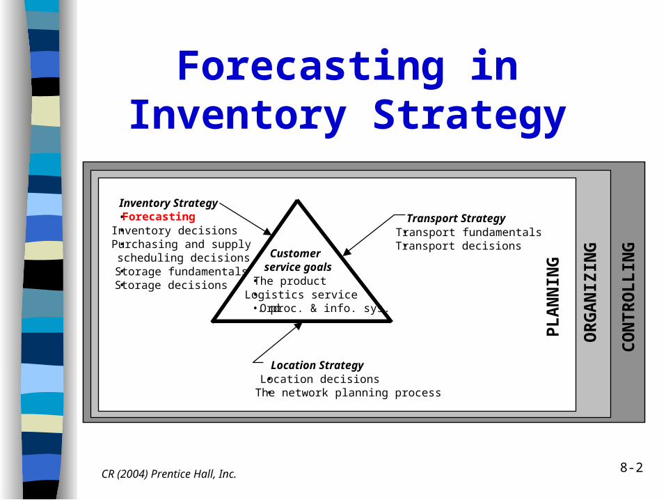
Forecasting in Inventory Strategy
CR (2004) Prentice Hall, Inc.
PL
AN
NIN
G
OR
GA
NIZ
ING
CO
NT
RO
LL
ING
Transport Strategy• Transport fundamentals• Transport decisions
Customer service goals
• The product• Logistics service• Ord. proc. & info. sys.
Inventory Strategy• Forecasting• Inventory decisions• Purchasing and supply
scheduling decisions• Storage fundamentals• Storage decisions
Location Strategy• Location decisions• The network planning process
8-3
What’s Forecasted in the Supply Chain?
•Demand, sales or requirements
•Purchase prices
•Replenishment and delivery times
CR (2004) Prentice Hall, Inc.
8-4CR (2004) Prentice Hall, Inc.
Some Forecasting Method Choices
•Historical projectionMoving averageExponential smoothing
•Causal or associativeRegression analysis
•QualitativeSurveysExpert systems or rule-based
•Collaborative

8-5CR (2004) Prentice Hall, Inc.
Typical Time Series Patterns:Random
0
50
100
150
200
250
0 5 10 15 20 25
Time
Sa
les
Actual salesAverage sales
8-6CR (2004) Prentice Hall, Inc.
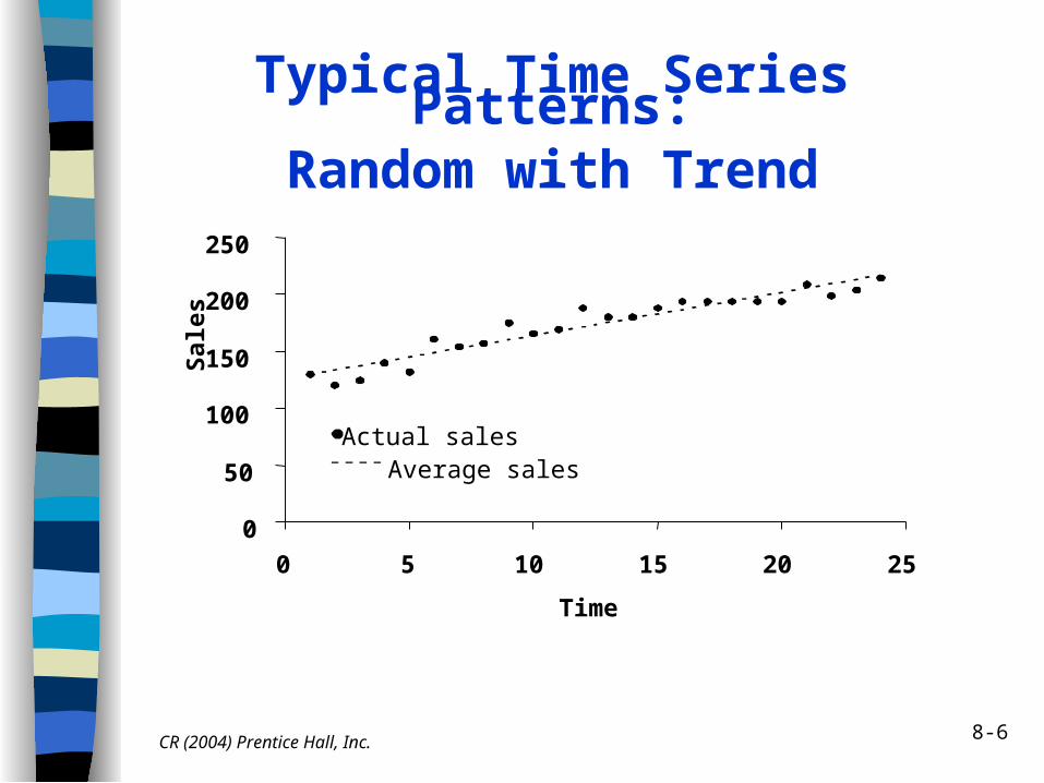
Typical Time Series Patterns:Random with Trend
0
50
100
150
200
250
0 5 10 15 20 25
Time
Sa
les
Actual salesAverage sales
8-7CR (2004) Prentice Hall, Inc.
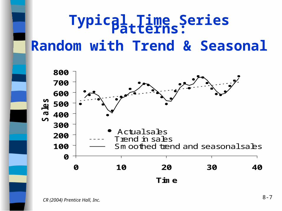
Typical Time Series Patterns:Random with Trend & Seasonal
0
100
200
300
400
500
600
700
800
0 10 20 30 40
Time
Sa
les
Actual salesTrend in salesSmoothed trend and seasonal sales
8-8CR (2004) Prentice Hall, Inc.
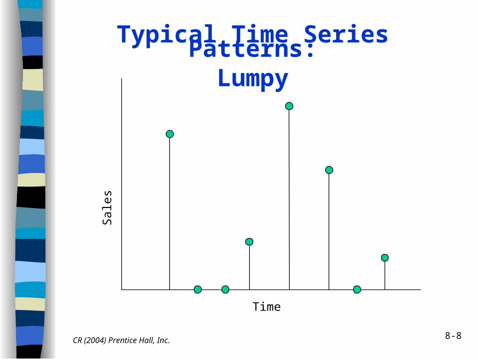
Typical Time Series Patterns:Lumpy
Time
Sal
es
8-9CR (2004) Prentice Hall, Inc.
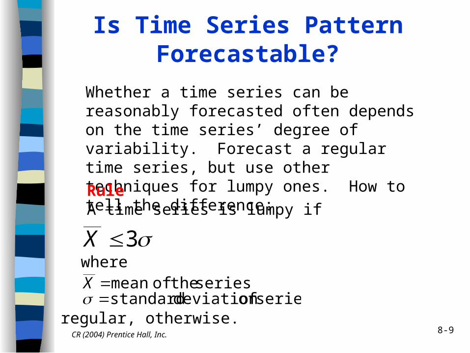
Is Time Series PatternForecastable?
Whether a time series can be reasonably forecasted often depends on the time series’ degree of variability. Forecast a regular time series, but use other techniques for lumpy ones. How to tell the difference:
RuleA time series is lumpy if
3Xwhere
series, of deviation standard series the of mean
X
regular, otherwise.
8-10
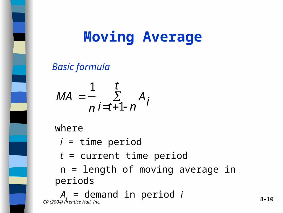
Moving Average
Basic formula
t
nti iAn
MA1
1
where
i = time period
t = current time period
n = length of moving average in periods
Ai = demand in period i
CR (2004) Prentice Hall, Inc.
8-11
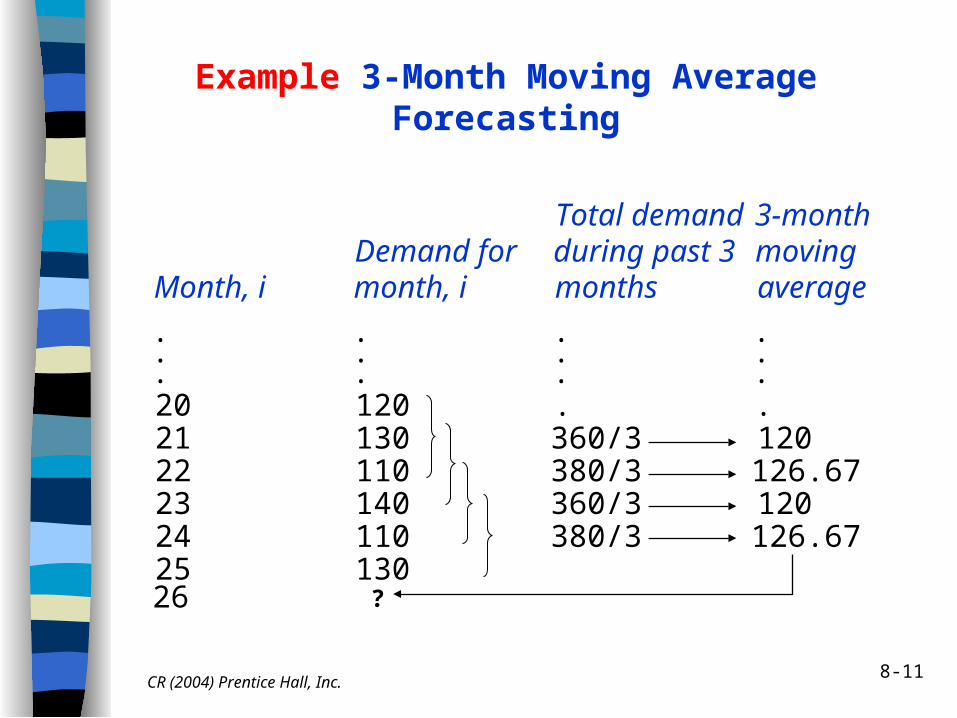
Example 3-Month Moving Average Forecasting
Month, iDemand formonth, i
Total demandduring past 3months
3-monthmovingaverage
.
.
....
.
.
....
20 120 . .21 130 360/3 12022 110 380/3 126.6723 140 360/3 12024 110 380/3 126.6725 13026 ?
CR (2004) Prentice Hall, Inc.
8-12
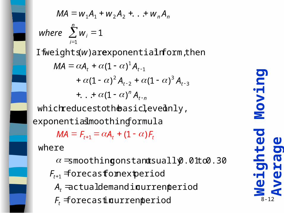
Wei
gh
ted
Mo
vin
g A
vera
ge
period current in forecast
period current in demand actual
period next for forecast
0.30 to 0.01 usually constant smoothing
where
)1(
formula smoothing exponential
only, level basic, the to reduces which
)1(...
)1()1(
)1(
then form, in exponential are )( weightsIf
1
...
1
1
33
22
11
1
2211
t
t
t
ttt
ntn
tt
tt
n
ii
nn
F
A
F
FAFMA
A
AA
AAMA
w
wwhere
AwAwAwMA
8-13
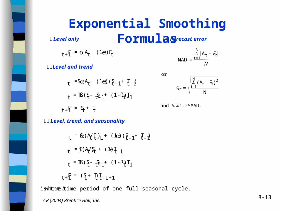
I. Level only
Ft+1 = At + (1-)Ft
II. Level and trend
St = At + (1-)(St-1 + Tt-1)
Tt = ß(St - St-1) + (1-ß)Tt-1
Ft+1 = St + Tt
III. Level, trend, and seasonality
St = (At/It-L) + (1-)(St-1 + Tt-1)
It = (At/St) + (1-)It-L
Tt = ß(St - St-1) + (1-ß)Tt-1
Ft+1 = (St + Tt)It-L+1
where L is the time period of one full seasonal cycle.
IV. Forecast error
MAD =|A t
F
N
tt
N|
1
or
S(A F )
NF
t t2
t 1
N
and SF 1.25MAD.
Exponential Smoothing Formulas
CR (2004) Prentice Hall, Inc.
8-14CR (2004) Prentice Hall, Inc.
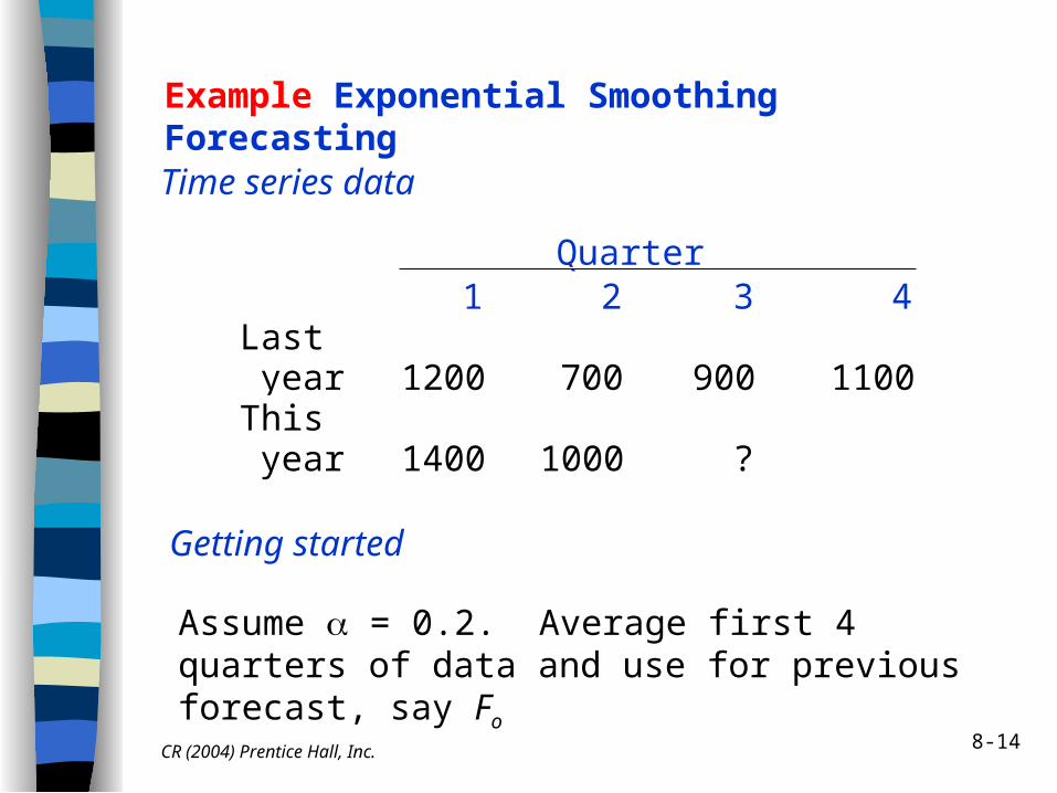
Example Exponential Smoothing Forecasting
Time series data
1 2 3 4Last year 1200 700 900 1100This year 1400 1000 ?
Quarter
Getting started
Assume = 0.2. Average first 4 quarters of data and use for previous forecast, say Fo
8-15CR (2004) Prentice Hall, Inc.
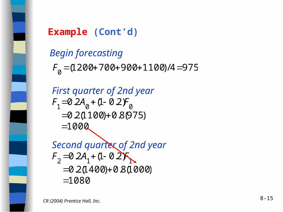
Example (Cont’d)
Begin forecasting
9754/)11009007001200(0
F
First quarter of 2nd year
1000)975(8.0)1100(2.0
)2.01(2.0001
FAF
Second quarter of 2nd year
1080)1000(8.0)1400(2.0
)2.01(2.0112
FAF

8-16CR (2004) Prentice Hall, Inc.
Example (Cont’d)
Third quarter of 2nd year
1064)1080(8.0)1000(2.0
)2.01(2.0023
FAF
Summarizing
1 2 3 4Last year 1200 700 900 1100This year 1400 1000 ?Fore- cast 1000 1080 1064
Quarter
8-17CR (2004) Prentice Hall, Inc.
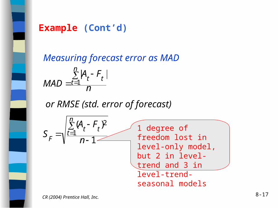
Example (Cont’d)
Measuring forecast error as MAD
or RMSE (std. error of forecast)
n
FAMAD
n
ttt
1||
1
)(1
2
n
FAS
n
ttt
F
1 degree of freedom lost in level-only model, but 2 in level-trend and 3 in level-trend-seasonal models
8-18CR (2004) Prentice Hall, Inc.
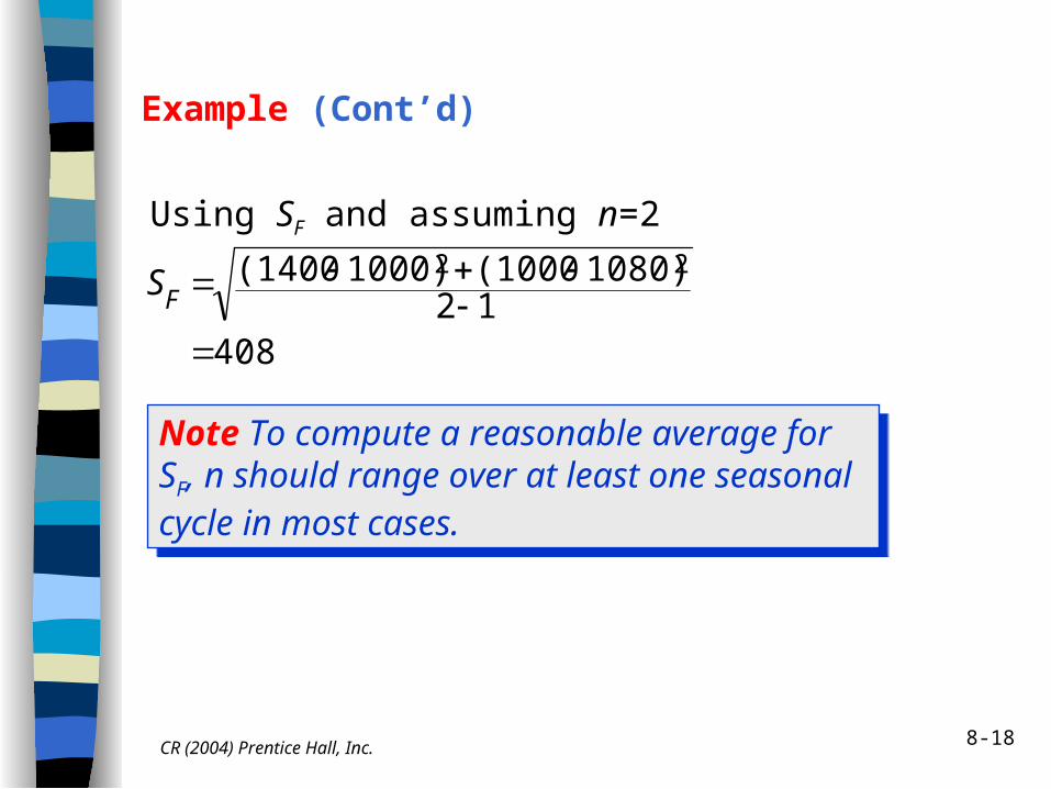
Example (Cont’d)
Using SF and assuming n=2
40812
1080)(10001000)(1400 22
FS
Note To compute a reasonable average for SF, n should range over at least one seasonal cycle in most cases.
Note To compute a reasonable average for SF, n should range over at least one seasonal cycle in most cases.
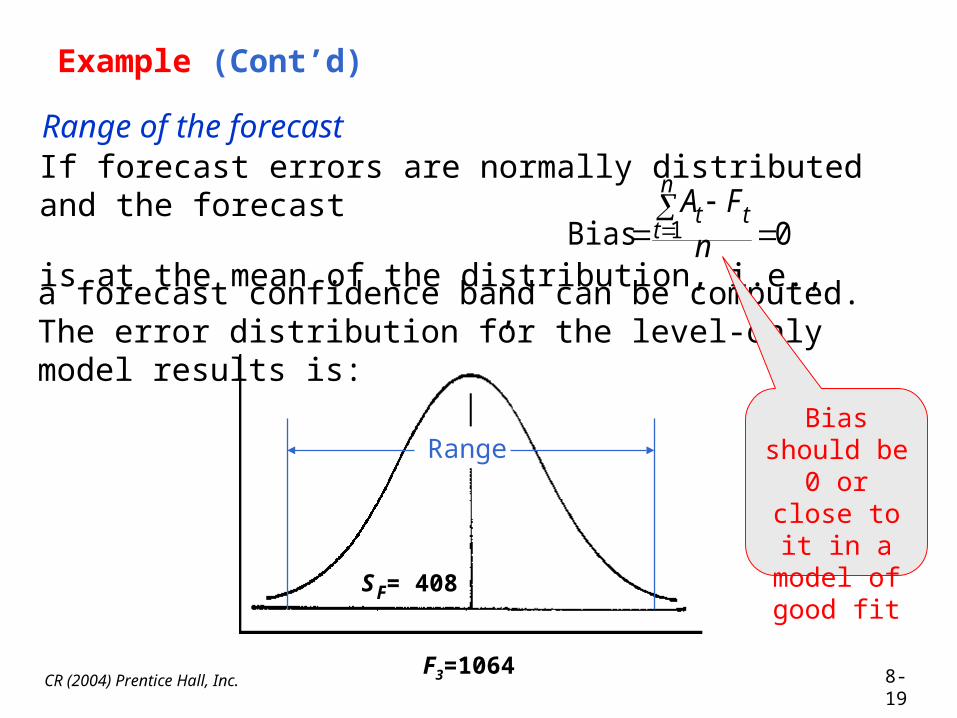
SF= 408
Example (Cont’d)
Range of the forecast
0Bias
n
FAn
ttt
1
F3=1064
Range
If forecast errors are normally distributed and the forecast
is at the mean of the distribution, i.e., ,
a forecast confidence band can be computed. The error distribution for the level-only model results is:
Bias should be 0 or
close to it in a model of
good fit
CR (2004) Prentice Hall, Inc. 8-19
8-20CR (2004) Prentice Hall, Inc.
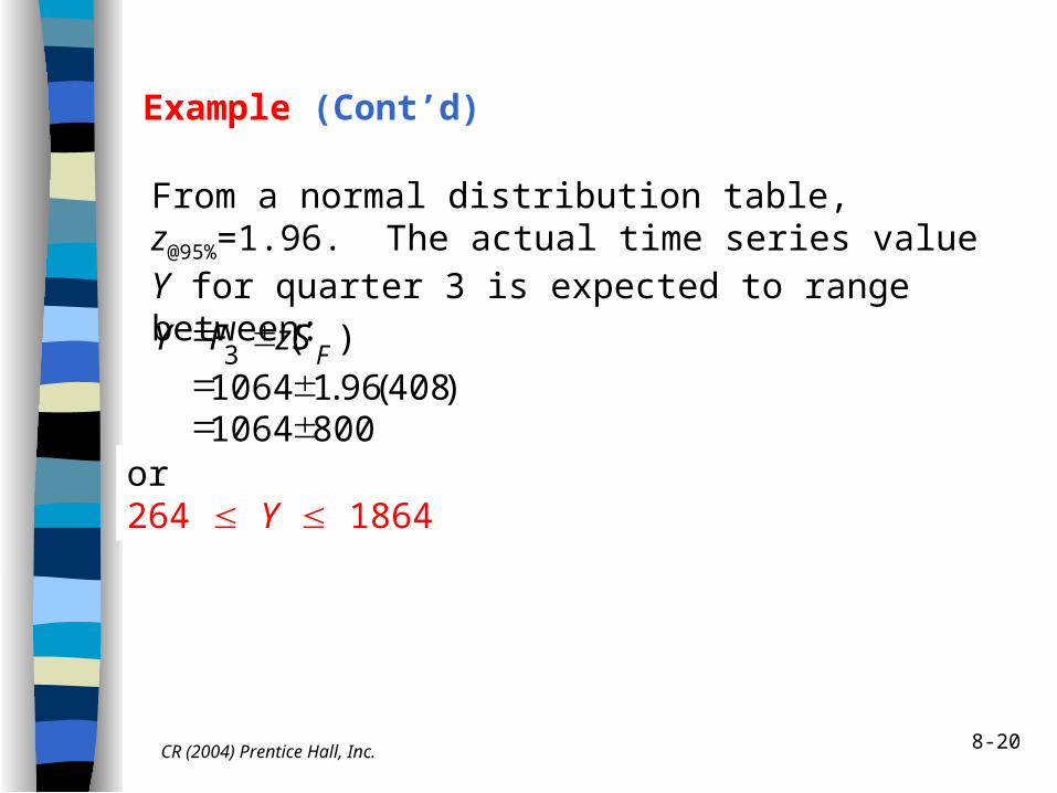
Example (Cont’d)
From a normal distribution table, z@95%=1.96. The actual time series value Y for quarter 3 is expected to range between:
or264 Y 1864
8001064)408(96.11064
)(3
F
SzFY
8-21CR (2004) Prentice Hall, Inc.
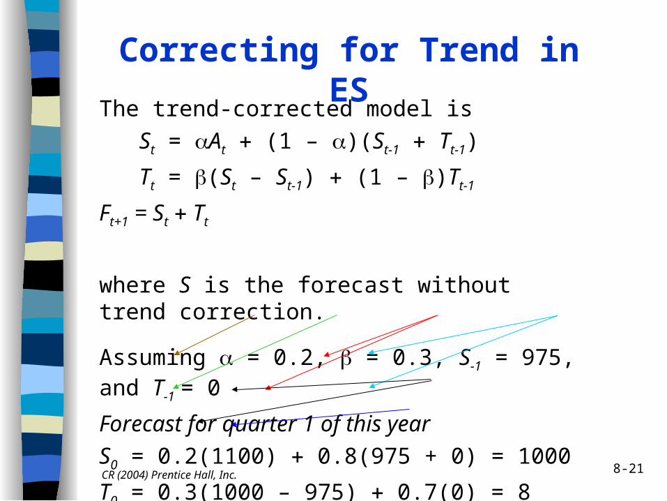
Correcting for Trend in ES
The trend-corrected model is
St = At (1 – )(St-1 Tt-1)
Tt = (St – St-1) (1 – )Tt-1
Ft+1 = St Tt
where S is the forecast without trend correction.
Assuming = 0.2, = 0.3, S-1 = 975, and T-1 = 0
Forecast for quarter 1 of this year
S0 = 0.2(1100) 0.8(975 + 0) = 1000
T0 = 0.3(1000 – 975) 0.7(0) = 8
F1 = 1000 8 = 1008

8-22
Forecast for quarter 2 of this year
S0 T0
S1 = 0.2(1400) 0.8(1000 8) = 1086.4
T1 = 0.3(1086.4 – 1000) 0.7(8) = 31.5
F2 = 1086.4 31.5 = 1117.9
Forecast for quarter 3 of this year
S2 = 0.2(1000) 0.8(1086.4 31.5) = 1094.3
T2 = 0.3(1094.3 – 1086.4) 0.7(31.5) = 24.4
F3 = 1094.3 24.4 = 1118.7, or 1119
CR (2004) Prentice Hall, Inc.
Correcting for Trend in ES (Cont’d)
8-23CR (2004) Prentice Hall, Inc.
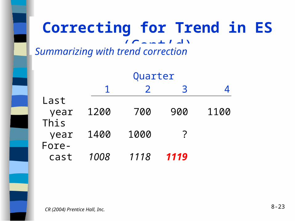
Correcting for Trend in ES (Cont’d)
Summarizing with trend correction
1 2 3 4Last year 1200 700 900 1100This year 1400 1000 ?Fore- cast 1008 1118 1119
Quarter
0 1
Fore-casterror
CR (2004) Prentice Hall, Inc.
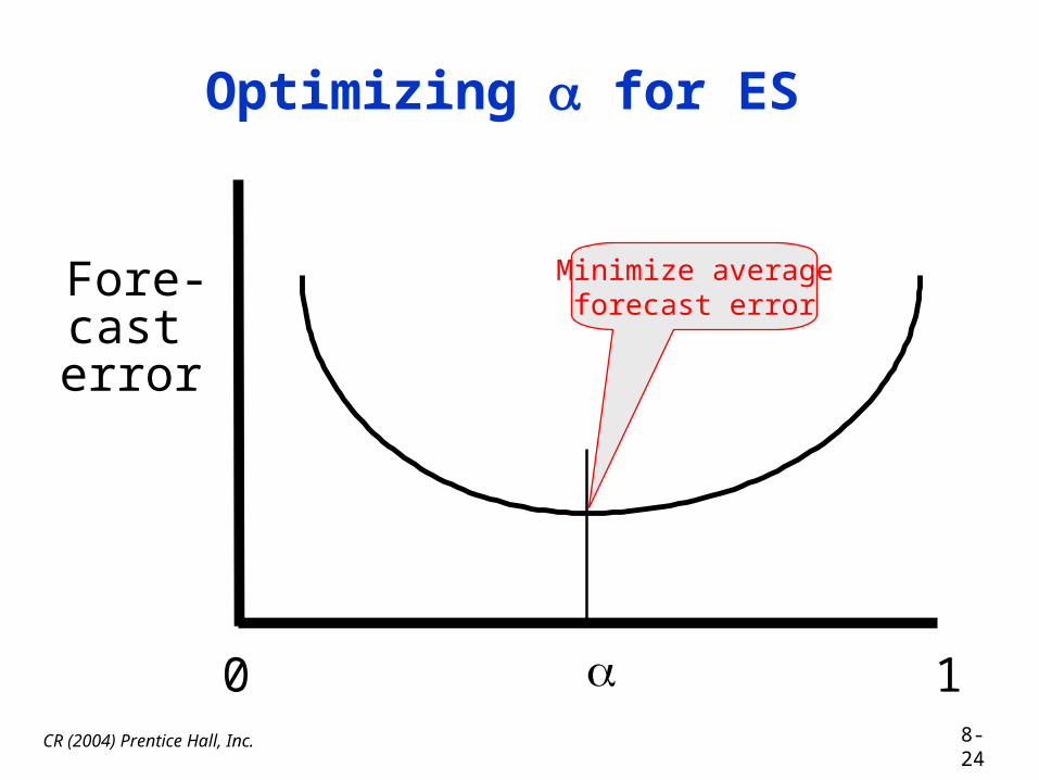
Optimizing for ES
Minimize averageforecast error
8-24

CR (2004) Prentice Hall, Inc.
Controlling Model Fit in ES
MSEFA
tt
signal Tracking
Tracking signal monitors the fit of the model to detect when the model no longer accurately represents the data
where the Mean Squared Error (MSE) is
nt
Ft
AMSE
n
t
1
2)(
If tracking signal exceeds a specified value (control limit), revise smoothing constant(s).
n is a reasonable numberof past periods depending
on the application
8-25
8-26
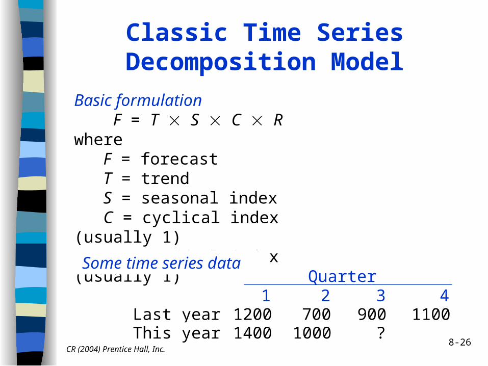
Classic Time Series Decomposition Model
Basic formulation F = T S C Rwhere F = forecast T = trend S = seasonal index C = cyclical index (usually 1) R = residual index (usually 1)
Some time series data
1 2 3 4Last year 1200 700 900 1100This year 1400 1000 ?
Quarter
CR (2004) Prentice Hall, Inc.

8-27CR (2004) Prentice Hall, Inc.
Classic Time Series Decomposition Model (Cont’d)
Trend estimation
Use simple regression analysis to find the trend equation of the form T = a bt. Recall the basic formulas:
22 tnt
tYnYtb
and
tbYa
8-28CR (2004) Prentice Hall, Inc.
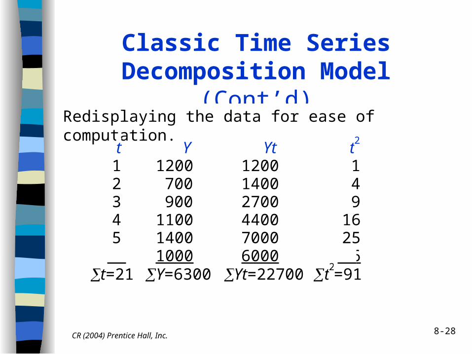
Classic Time Series Decomposition Model (Cont’d)
Redisplaying the data for ease of computation.
t Y Yt t2
1 1200 1200 12 700 1400 43 900 2700 94 1100 4400 165 1400 7000 256 1000 6000 36
t=21 Y=6300 Yt=22700 t2=91

8-29
Classic Time Series Decomposition Model (Cont’d)
Hence,
and
then
26(21/6)9100/6)6(21/6)(6322700
b
920.01)37.14(21/66
6300 a
T = 920.01 27.14t
Forecast for 3rd quarter of this year is:
T = 920.01 37.14(7) = 1179.99CR (2004) Prentice Hall, Inc.
8-30CR (2004) Prentice Hall, Inc.
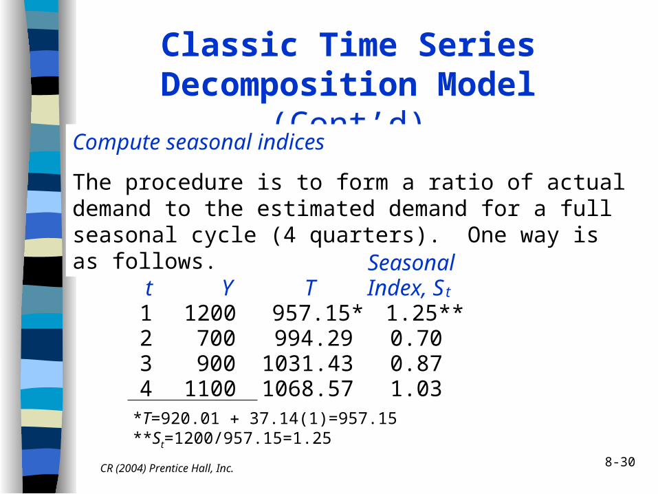
Classic Time Series Decomposition Model (Cont’d)
Compute seasonal indices
The procedure is to form a ratio of actual demand to the estimated demand for a full seasonal cycle (4 quarters). One way is as follows.
t Y TSeasonalIndex, St
1 1200 957.15* 1.25**2 700 994.29 0.703 900 1031.43 0.874 1100 1068.57 1.03
*T=920.01 37.14(1)=957.15**St=1200/957.15=1.25
8-31CR (2004) Prentice Hall, Inc.
Classic Time Series Decomposition Model (Cont’d)
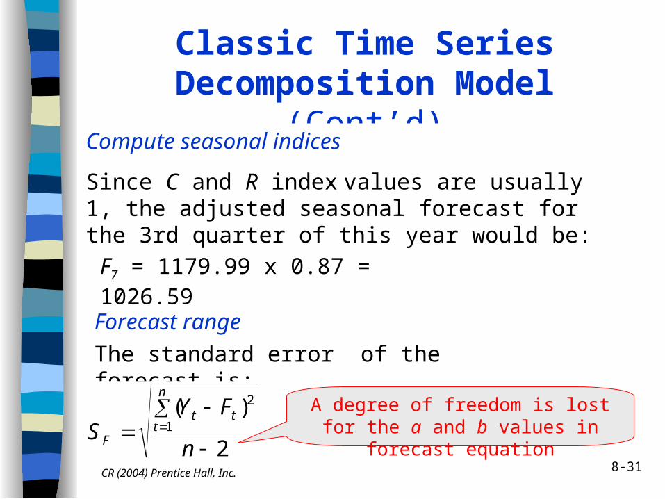
Compute seasonal indices
Since C and R index values are usually 1, the adjusted seasonal forecast for the 3rd quarter of this year would be:
F7 = 1179.99 x 0.87 = 1026.59
Forecast range
The standard error of the forecast is:
2
)(1
2
n
FYS
n
ttt
F
A degree of freedom is lost for the a and b values in forecast equation
8-32CR (2004) Prentice Hall, Inc.
Classic Time Series Decomposition Model (Cont’d)
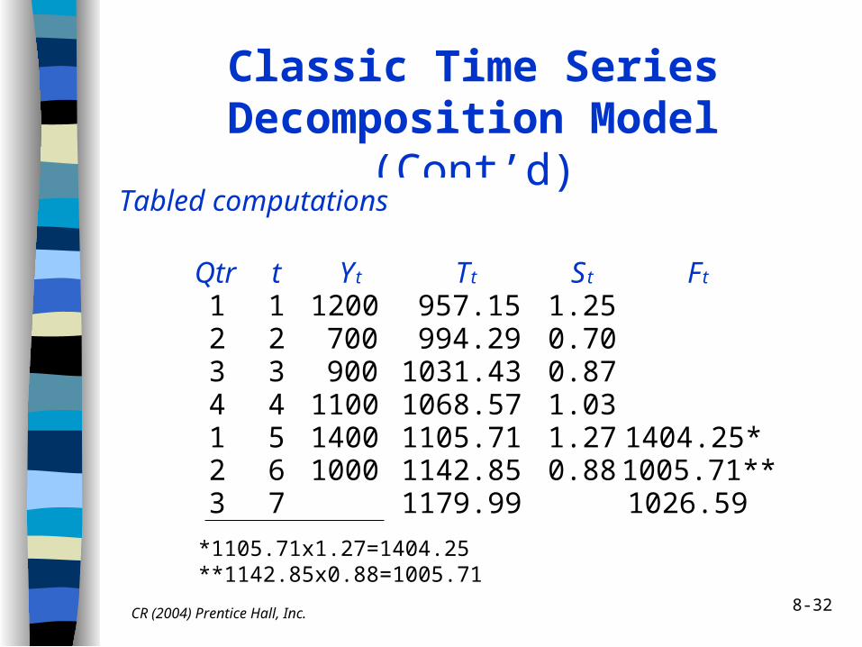
Qtr t Yt Tt St Ft
1 1 1200 957.15 1.252 2 700 994.29 0.703 3 900 1031.43 0.874 4 1100 1068.57 1.031 5 1400 1105.71 1.27 1404.25*2 6 1000 1142.85 0.88 1005.71**3 7 1179.99 1026.59
*1105.71x1.27=1404.25**1142.85x0.88=1005.71
Tabled computations
8-33CR (2004) Prentice Hall, Inc.
Classic Time Series Decomposition Model (Cont’d)
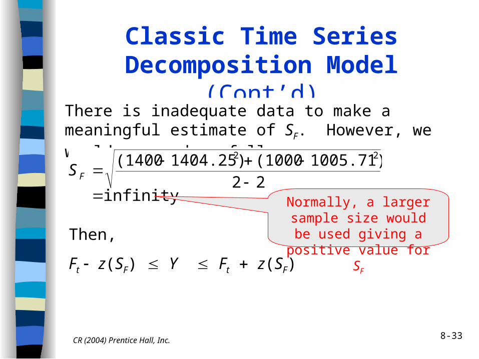
There is inadequate data to make a meaningful estimate of SF. However, we would proceed as follows:
infinity 22
1005.71)(10001404.25)(1400 22
FS
Then,
Ft z(SF) Y Ft z(SF)
Normally, a larger sample size would be used giving
a positive value for SF
8-34CR (2004) Prentice Hall, Inc.
Regression Analysis
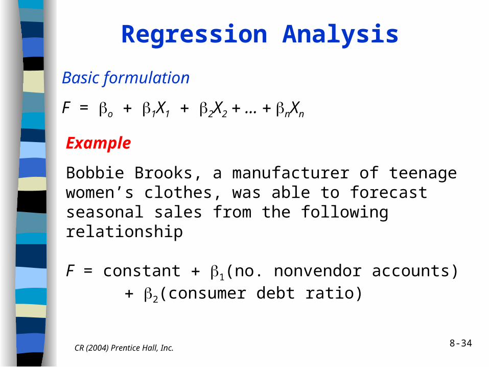
Basic formulation
F = o 1X1 2X2 … nXn
Example
Bobbie Brooks, a manufacturer of teenage women’s clothes, was able to forecast seasonal sales from the following relationship
F = constant 1(no. nonvendor accounts) 2(consumer debt ratio)
CR (2004) Prentice Hall, Inc.
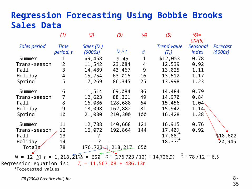
Sales period
(1)
Timeperiod, t
(2)
Sales (Dt )($000s)
(3)
Dt t
(4)
t2
(5)
Trend value(Tt )
(6)=(2)/(5)
Seasonalindex
Forecast($000s)
Summer 1 $9,458 9,458
1 $12,053 0.78Trans-season 2 11,542 23,084 4 12,539 0.92Fall 3 14,489 43,467 9 13,025 1.11Holiday 4 15,754 63,016 16 13,512 1.17Spring 5 17,269 86,345 25 13,998 1.23
Summer 6 11,514 69,084 36 14,484 0.79Trans-season 7 12,623 88,361 49 14,970 0.84Fall 8 16,086 128,688 64 15,456 1.04Holiday 9 18,098 162,882 81 15,942 1.14Spring 10 21,030 210,300 100 16,428 1.28
Summer 11 12,788 140,668 121 16,915 0.76Trans-season 12 16,072 192,864 144 17,401 0.92Fall 13 ? 17,887* $18,602Holiday 14 ? 18,373* 20,945
Totals 78 176,723 1,218,217 650
Regression Forecasting Using Bobbie Brooks Sales Data
N = 12 Dt t = 1,218,217 t2 = 650 = =( , / ) , .176 723 12 14 726 92 = =78 12 6 5/ .Regression equation is: Tt = 11,567.08 + 486.13t *Forecasted values
D t
8-35
8-36
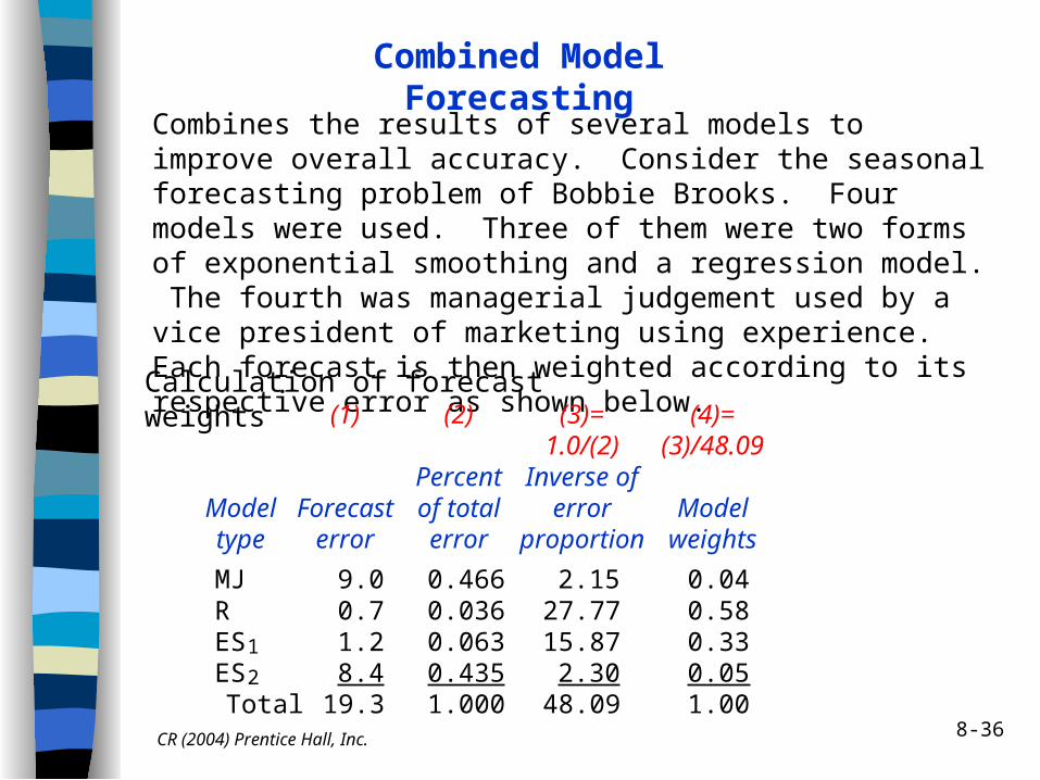
Combined Model Forecasting
Combines the results of several models to improve overall accuracy. Consider the seasonal forecasting problem of Bobbie Brooks. Four models were used. Three of them were two forms of exponential smoothing and a regression model. The fourth was managerial judgement used by a vice president of marketing using experience. Each forecast is then weighted according to its respective error as shown below.
Calculation of forecast weights
Modeltype
(1)
Forecasterror
(2)
Percentof totalerror
(3)=1.0/(2)
Inverse oferror
proportion
(4)=(3)/48.09
Modelweights
MJ 9.0 0.466 2.15 0.04R 0.7 0.036 27.77 0.58ES1 1.2 0.063 15.87 0.33ES2 8.4 0.435 2.30 0.05 Total 19.3 1.000 48.09 1.00
CR (2004) Prentice Hall, Inc.
8-37
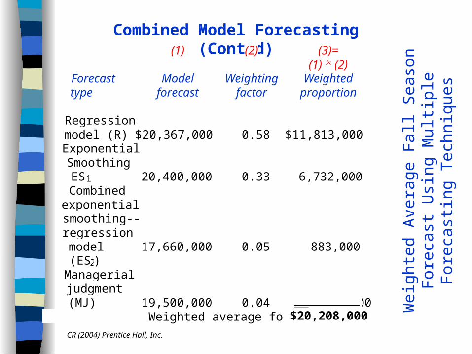
Combined Model Forecasting (Cont’d)
Wei
ghte
d A
vera
ge F
all S
easo
n F
orec
ast
Usi
ng M
ultip
le F
orec
astin
g T
echn
ique
s
Forecasttype
(1)
Modelforecast
(2)
Weightingfactor
(3)=(1) (2)
Weightedproportion
Regressionmodel (R) $20,367,000 0.58 $11,813,000ExponentialSmoothingES1 20,400,000 0.33 6,732,000Combinedexponentialsmoothing--regressionmodel(ES2)
17,660,000 0.05 883,000
Managerialjudgment(MJ) 19,500,000 0.04 780,000
Weighted average forecast $20,208,000
CR (2004) Prentice Hall, Inc.
CR (2004) Prentice Hall, Inc.
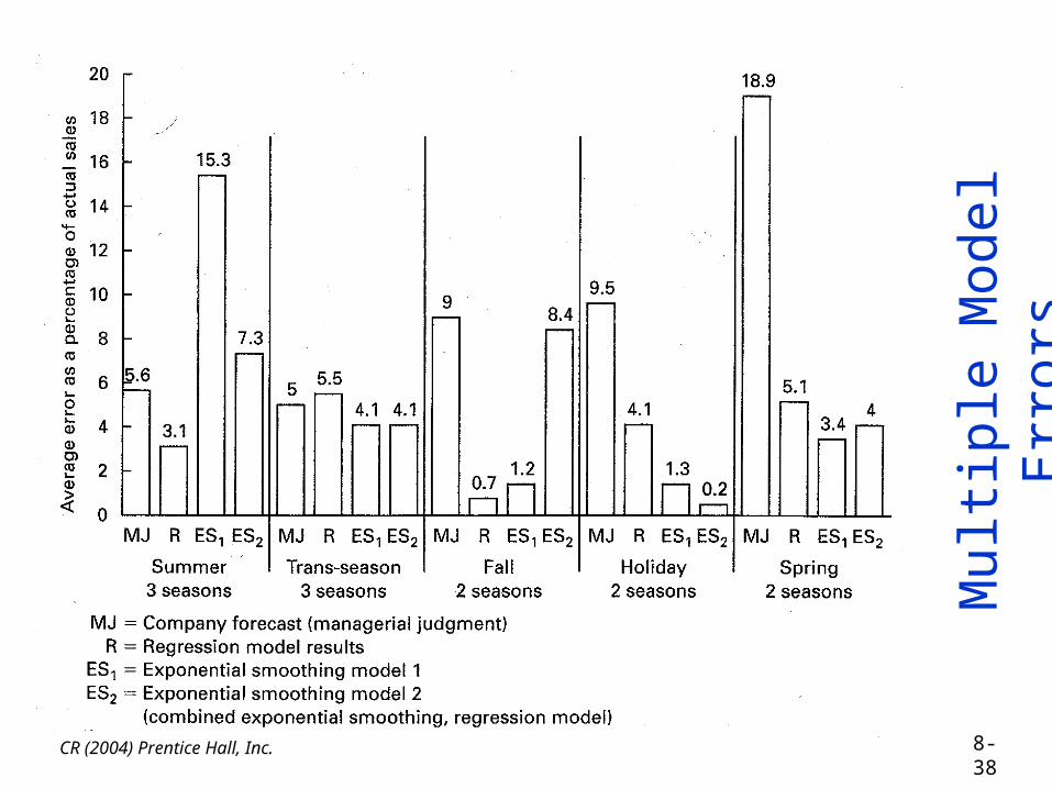
Mul
tiple
Mod
el E
rror
s
8-38
8-39CR (2004) Prentice Hall, Inc.
Actions When Forecasting is Not Appropriate
Seek information directly from customers
Collaborate with other channel members
Apply forecasting methods with caution (may work where forecast accuracy is not critical)
Delay supply response until demand becomes clear
Shift demand to other periods for better supply response
Develop quick response and flexible supply systems
8-40CR (2004) Prentice Hall, Inc.
Collaborative Forecasting
• Demand is lumpy or highly uncertain• Involves multiple participants each with
a unique perspective—“two heads are better than one”
• Goal is to reduce forecast error• The forecasting process is inherently
unstable
8-41CR (2004) Prentice Hall, Inc.
Collaborative Forecasting: Key Steps
•Establish a process champion
• Identify the needed Information and collection processes
•Establish methods for processing information from multiple sources and the weights assigned to multiple forecasts
•Create methods for translating forecast into form needed by each party
•Establish process for revising and updating forecast in real time
•Create methods for appraising the forecast
•Show that the benefits of collaborative forecasting are obvious and real
8-42CR (2004) Prentice Hall, Inc.
Managing Highly Uncertain Demand
Delay forecasting as long as possible
Prioritize supply by product’s degree of uncertainty (supply to the more certain products first)
Apply the principle of postponement to the most uncertain products (delay committing to a final product form until an order is received)
Create flexible supply to changing demand (alter capacity and output rates through subcontracting, computer technology, multi-purpose processes, etc.)
Be able to respond quickly to uncertain demand levels