©Det här verket är upphovrättskyddat enligt Lagen (1960:729) om upphovsrätt till litterära och konstnärliga verk. Det har digitaliserats med stöd av Kap. 1, 16 § första stycket p 1, för forsk-ningsändamål, och får inte spridas vidare till allmänheten utan upphovsrättsinehavarens medgivande.

Alla tryckta texter är OCR-tolkade till maskinläsbar text. Det betyder att du kan söka och kopie-ra texten från dokumentet. Vissa äldre dokument med dåligt tryck kan vara svåra att OCR-tolka korrekt vilket medför att den OCR-tolkade texten kan innehålla fel och därför bör man visuellt jämföra med verkets bilder för att avgöra vad som är riktigt.

This work is protected by Swedish Copyright Law (Lagen (1960:729) om upphovsrätt till litterära och konstnärliga verk). It has been digitized with support of Kap. 1, 16 § första stycket p 1, for scientific purpose, and may no be dissiminated to the public without consent of the copyright holder.

All printed texts have been OCR-processed and converted to machine readable text. This means that you can search and copy text from the document. Some early printed books are hard to OCR-process correctly and the text may contain errors, so one should always visually compare it with the images to determine what is correct.

01

23

45

67

89

1011

1213

1415

1617

1819

20 21

2223

2425

2627

2829

30CM

01

23

45

67

89

1011

12INCH

EARTH SCIENCES CENTRE GÖTEBORG UNIVERSITY A1042006

COASTALLY TRAPPED WAVES AND CURRENTS

Olof H. Dahl

Department of Oceanography GÖTEBORG 2006

Coastally trapped waves and currents

Olof H. Dahl

Akademisk avhandling

För vinnande av filosofie doktorsexamen i Oceanografi (examinator Professor Anders Stigebrandt) som enligt beslut av

Lärarförslagsnämnden för Geovetenskaper vid Göteborgs universitet kommer att offentligt försvaras onsdagen den 31:e maj 2006, kl 10.15

i Hörsalen, Geovetarcentrum, Guldhedsgatan 5 A, Göteborg.

Fakultetsopponent är Senior Scientist Dr. Michael A. Spall, Woods Hole Océanographie Institution, USA.

Abstract

Coastal currents are important agents for the transport of heat, salt and other properties in the ocean. Generation and dynamics of coastal currents are investigated, including the role of c oastally trapped waves, with focus on four specific problems.

In the presence of a sloping bottom it was found that a buoyant coastal current that gradually loses its buoyancy along the coast can be described completely with geostrophic dynamics. The along-coast density gradient drives a geostrophic flow towards the coast, generating a barotropic current along the coast, parallel to the depth contours. Thus a coastal current can retain its transport along the coast without deepening. The theoretical pre­dictions were compared with numerical experiments mimicking the Nordic Seas using simplified forcing and topography A sloping bottom is essen­tial since geostrophic dynamics are not enough to describe a similar current along a vertical wall.

The propagation and structure of perturbations on a buoyant coastal current along a vertical wall was investigated. Using a 1 1/2-layer model, analytical solutions were derived in two cases; a current with no horizontal shear in the buoyant layer and a current with constant potential vorticity.

A theory for the transient establishment of barotropic coastal currents along closed depth contours was derived. With local forcing, the response can be described as a sum of t opographic waves, the mean along-contour acceleration and a stationary recirculating part.

The difference between the response to cyclonic and anticyclonic forcing in a closed basin was investigated using a numerical model. It was found that although the cyclonic response remained undisturbed, the anticyclonic response was severely reduced by along-coast variations in the bottom slope. The cyclonic response was stationary and well d escribed by linear theory, while the anticyclonic response deviated substantially from linear theory and never reached a steady state.

Key words: Coastal currents, trapped waves, JEBAR, ocean circulation stability.

Coastally trapped waves and currents

Olof H. Dahl

Göteborg 2006

Department of Oceanography Earth Sciences Centre Göteborg University Göteborg, Sweden

A104/2006, ISSN 1400-3813

Olof H. Dahl Coastally trapped waves and currents

A104 2006 ISSN 1400-3813 Distribution: Earth Sciences Centre, Göteborg, Sweden ©Olof H. Dahl

...the world of men could be divided into three groups: those living, those dead, and those at sea.

-Guy Gavriel Kay The Last Light of the Sun

Abstract

Coastal currents are important agents for the transport of heat, salt and other properties in the ocean. Generation and dynamics of coastal currents are investigated, including the role of co astally trapped waves, with focus on four specific p roblems.

In the presence of a sloping bottom it was found that a buoyant coastal current that gradually loses i ts buoyancy along the coast can be described completely with geostrophic dynamics. The along-coast density gradient drives a geostrophic flow towards the coast, generating a barotropic current along the coast, parallel to the depth contours. Thus a coastal current can retain its transport along the coast without deepening. The theoretical pre­dictions were compared with numerical experiments mimicking the Nordic Seas using simplified forcing and topography. A sloping bottom is essen­tial since geostrophic dynamics are not enough to describe a similar current along a vertical wall.

The propagation and structure of perturbations on a buoyant coastal current along a vertical wall was investigated. Using a 1 1/2-layer model, analytical solutions were derived in two cases; a current with no horizontal shear in the buoyant layer and a current with constant potential vorticity.

A theory for the transient establishment of b arotropic coastal currents along closed depth contours was derived. With local forcing, the response can be described as a sum of topographic waves, the mean along-contour acceleration and a stationary recirculating part.

The difference between the response to cyclonic and anticyclonic forcing in a closed basin was investigated using a numerical model. It was found that although the cyclonic response remained undisturbed, the anticyclonic response was severely reduced by along-coast variations in the bottom slope. The cyclonic response was stationary and well d escribed by linear theory, while the anticyclonic response deviated substantially from linear theory and never reached a steady state.

Key words: Coastal currents, trapped waves, JEBAR, ocean circulation stability.

Preface

This thesis contains a summary (Part I) and four appended papers (Part II). In the summary, the papers are referred to by their Roman numerals.

Paper I: G. Walin, G. Broström, J. Nilsson and O. Dahl, 2004: Baroclinic boundary currents with downstream decreasing buoyancy: A study of a n idealized Nordic Seas system. Journal of M arine Research 62, 517-543.

Paper II: O. H. Dahl, 2005: Development of p erturbations on a buoyant coastal current. Journal of Fluid Mechanics 527, 337-351.

Paper III: O. H. Dahl and G. Walin, 2006: On the generation of slope currents from local forcing. Submitted to Journal of Marine Research.

Paper IV: O. H. Dahl, 2006: On the preference for cyclonic topographically trapped circulation. Submitted to Journal of Physical Oceanography.

Paper I is the result of disc ussions, initiated by Walin, strung out over several years between the four authors. Nilsson gave important theoretical input. Walin and Nilsson did the most of the writing. Broström provided the numerical experiments and wrote Section 2. Dahl gave theoretical input, did most of t he analysis of th e model output, and contributed to the design of t he numerical experiments and the writing.

Paper III is based on an idea hatched by Walin, and was written in close collaboration between Dahl and Walin. Dahl was responsible for the writing and the theoretical analysis, with large contributions from Walin.

Contents

I Summary 1

1 Introduction 2

2 Geostrophic motion in a stratified ocean 5 2.1 How to represent the flow 7

3 Stationary coastal currents 9 3.1 Non-linearities and the preference for cyclonic flow 11 3.2 Consequences of a flat bottom and vertical side walls .... 13

4 Time dependency in coastal currents 14 4.1 Establishment of a coastal current 14 4.2 Perturbations on baroclinic currents . 16

5 Future outlook 18

A Appendix 21

II Papers I-IV 25

Part I

Summary

1 Introduction

There are two ways the presence of a coastline can lead to a current along the coast:

(a) Winds transporting water away from or towards the coast.

(b) Accumulation of bu oyant (less dense) water along the coast.

Both of the se processes lead to a gradient in the pressure between the open ocean and the coastal water. The pressure gradient will cause water to flow from high pressure towards low pressure. Because of t he Earth's rotation, however, the flow will veer off to the right (on the Northern Hemisphere) until the pressure force is balanced by the Coriolis force in the opposite direction. When these two forces balance each other, the flow is geostrophic, and in the case of a coastal current, parallel to the coast.

We will now d iscuss the two generating mechanisms. Case (a): In a classic paper Ekman (1905) showed that the net trans­

port of wate r forced by wind is directed 90° to the right of the wind (on the Northern Hemisphere). Furthermore he showed that this Ekman transport takes place in a thin surface layer (tens of meters thick, c.f. Nerheim & Stigebrandt 2006), the surface Ekman layer. There is a similar layer at the bottom of the ocean, caused by friction; the bottom Ekman layer.

Now, if the wind has a component parallel to the coast, the Ekman transport will move water towards/away from the coast. As a result the sea level at the coast will rise/sink, establishing a pressure gradient between the coast and the open ocean, giving rise to a geostrophic current parallel to the coast, as discussed above. This is illustrated in Figure 1.1a.

Case (b): Buoyant water can be accumulated at the coast either by outflow from rivers and marginal seas or by Ekman transport towards the coast. The pressure at a point is given by the mass of the water column above it. If water columns near the coast are less dense than columns further out, we will h ave a horizontal pressure gradient between the coast and the

Coastally trapped waves and currents 3

wind river inp«'* a) Q b)

\ buoyant water •=>

\ coastal A

dense \current

water \ •/•jär coastal current

Ekman transport

pressure gradient force <=• Coriolis force

Figure 1.1: a) A coastal current caused by wind driving water away from the coast,

b) A coastal current caused by the accumulation of buoyant water at the coast.

ocean which varies with depth. Figure 1.1b illustrates this for a case where the sea surface stands higher near the coast, yielding a coastal current in the upper buoyant layer.

Coastal currents transport heat, salt, and other properties in the ocean. In Figure 1.2 we show the salinity in the East Greenland Current from the AO -02 expedition 2002 (Rudels et al. 2005). The East Greenland Current is a good example of a buoyant coastal current, and carries relatively fresh water from the Arctic into the Atlantic. Currents like the East Greenland Current play a vital role in the thermohaline circulation, and thus for the whole climate system.

Coastally trapped waves a re important in the dynamics of co astal cur­rents. The waves can act as carriers of information - if t he structure of th e coastal current is changed at some point along the coast, the change will be transmitted along the coast by coastally trapped waves. Thus the travelling direction and structure of th e waves govern how a change will spread.

Coastal currents are often unstable, displaying meanders and tying off eddies, which opens for interesting aspects of waves and currents outside the scope of th is thesis.

This summary is organized as follows. Chapter 2 describes general fea­tures of geostrophic motion, and also contains a discussion of how buoyancy

4 Olof Dahl

E JZ

500 i—- p—— r , -1—1— / , '""32.5 0 50 100 150 200 250 300 350

Distance (km)

34 £• c

~cö 33.5 w

Figure 1.2: The salinity in the East Greenlan d Current between Greenland ( to the

left) and Iceland ( to the right), between 70°l\l and 66.8°N. The current runs close to

the Greenland coast, and transports fresher water southwards. Th e data are from t he

AO -02 expedition (Rudels et al. 2005).

driven currents are best described mathematically. In Chapter 3 station­ary coastal currents are discussed with special focus on the generation of coastal currents by along-coast buoyancy variations (Paper I) and the dif­ference between cyclonic and anti-cyclonic flow (Paper IV). A section of Chapter 3 is devoted to the difference between flow over flat and sloping bottom topography. Chapter 4 essentially contains summaries of P aper II and Paper III, and deals with the establishment of coastal currents (Paper III) and the propagation of s mall perturbations (Paper II). In Chapter 5 some possible extensions of the work presented in this thesis are suggested. As an appendix the mathematical notation used in this summary is listed.

2 Geostrophic motion in a stratified ocean

When the flow is strictly geostrophic, the pressure gradient is balanced by the Coriolis force and the velocity (u) is given by equation (9) from Paper I:

/

Z i k x Vqdz + ~qH k x VH + -,— k x Vp0(x,y), (2.1)

H J JPO

where H is the depth and po is a pressure field with arbitrary horizontal distribution, q is the density anomaly defin ed by p = (1 — q)pQ with q u

being the density anomaly at the bottom, i.e. at'J| — —H l. Note that the sea surface elevation ij is not explicitly given, but can be determined from pq an d the density distribution. In the case of a homogeneous fluid v — po/gpo-

All vertical dependence in the velocity is caused by the density distri­bution. Consequently, the only term on the right hand side of (2.1) with vertical variation is the first term. I will label this term the "thermal wind"2, since it constitutes the thermal wind velocity, with zero flow at the bottom.

The second and third terms on the right hand side of (2.1) are barotropic, i.e. they have no vertical variation. The second term represents the flow caused by interaction between stratification and topography, and will be labelled the " false barotropic" part of the flow. Note that the false barotropic velocity is always parallell to the depth contours, and faster over steep topography.

The third term will be called the "true barotropic" part, since it is not dependent on the density distribution. However, there is an ambiguity in

1For readability the most common variables are not defined in the text. All variables are however defined in the appendix.

2The thermal wind velocity is determined from the thermal wind equation: du/dz = g/fk x q, obtained by combining the geostrophic and hydrostatic equations.

6 Olof Dahl

po (dense) â i

™h 00

A (light)

Figure 2.1: The thermal wind and false barotropic velocities, in the case of along-

coast density variations. Grey arrows repres ent false barotropic velocities and black

arrows represe nt thermal wind velocities. Note that the false barotropic velocity is

greater over steeper slope a nd that it grows along the coast.

this representation of the barotropic part of flow, since t he false barotropic part is dependent on the reference density po- This means that if the refer­ence density po is incre ased, the false barotropic velocity will also increase, with a corresponding decrease in the true barotropic velocity.

The properties of the thermal wind and false barotropic flow are demon­strated with the following simple example, as illustrated in Figure 2.1. Con­sider a long straight sloping beach. The density is independent of depth and increases along the coast (with the coast to the right) from pi at one point to po at another. Thus, the thermal wind will move water towards the coast, from deeper to shallower water. This is compensated by a divergent false barotropic transport in the direction against the density gradient.

While the false barotropic term can be calculated from the density field and topography (although depending on the choice of the reference density po), the true barotropic term cannot be determined from the geostrophic relation alone. The addition of th e continuity equation puts constraints on the true barotropic term, which can then sometimes be calculated.

false barotropic

thermal wind

Coastally trapped waves and currents 7

The continuity equation3

^X Vy H" IVz — 0, (2.2)

can be rewritten in a more useful form by vertical integration. Wind forcing and bottom friction can then be introduced through the vertical velocity (w) at the surface and bottom as Ekman pumping. Thus the vertically integrated continuity equation can be written

uh • V-fiT = —V • (mT + in?,), (2.3)

for stationary flow on a f-plane4 . Here Uf, is the geostrophic velocity at the bottom and mT and m;, are the surface and bottom Ekman transports respectively. (This is done in more detail in e.g. Nilsson et al. (2005).) Note that only the true barotropic term in (2.1) contributes to the cross-isobath flow outside the Ekman layers, i.e.,

ub . VH = -L (k x Vp0(x, y)) . S7H. (2.4) J Po

Bear in mind that both the false and true barotropic velocities are needed to calculate the bottom Ekman transport m;,, which depends on the strength of the geostrophic bottom velocity u;,. (Remember that m/, is perpendicular to uj,.)

With (2.1) and (2.3) as the starting point some properties of coastal currents, especially the results from Papers I-IV, are discussed in Chapter 3 and 4.

2.1 How to represent the flow

When discussing the interaction of topography and stratification in e.g. coastal currents, the choice of representation of the flow is of importance for the understanding. The representation given by (2.1) is easy to interpret physically, and this is why it was chosen in Paper I. In this section two other ways of representing the flow will be discussed.

To obtain the pressure used to determine the geostrophic velocity at depth z, the hydrostatic equation5 is integrated vertically. In (2.1) we have

3The continuity equation states that mass is conserved, and in this formulation also that the fluid is incompressible.

4 On a /-plane there is no variation in the Coriolis parameter. This approximation holds for areas with small enough North-South extent.

5The hydrostatic equation states that the vertical pressure gradient is dependent on density only, i.e. dp/dz = pg. It is obtained from the vertical momentum equation by neglecting e.g. the vertical acceleration.

8 Olof Dahl

integrated the hydrostatic equation from the bottom to z . It is tempting to instead integrate from z to the sea surface, yielding

u - j k x V V ( x . ! j ) - ^ j \ m V q d z , (2.5)

where r j is the sea surface height. This representation suggests that the bottom velocity is dependent on the stratification above it, while our rep­resentation (2.1) suggests it is not. Which approach is correct depends on whether one argues that the sea surface height is causing flow (the common approach, leading to (2.5)), rather than being an effect of t he flow pattern (our approach). An example using (2.5) can be found in Csanady (1985).

Another common representation yields the "JEBAR" (Joint Effect of Baroclinicity and Relief) terms, often described as a forcing factor. Here I will d emonstrate that these terms appear as an effect of using the total horizontal transport instead of the explicit bottom velocity in (2.3). This is also shown by Mertz & Wright (1992), in a somewhat different way.

Define the horizontal transport U as ,o

U= / u d z . (2.6) J H

Since all parts of the flow are included in U, the contributions from the thermal wind velocity must be subtracted to obtain u& • Vif, appearing in (2.3). We are also allowed to subtract the false barotropic velocity, recalling that only the true barotropic flow contributes to the cross-isobath transport, thus obtaining

Ub • Vif

§'VH-(àkx H / V q d z + q H V H I - H

d z • Vif. (2.7)

The "JEBAR" terms are given by the second term on the right hand side of (2.7). The common form of the "JEBAR" terms are obtained through integration by parts and multiplication with //if, i.e.

Gr̂ i: c z

V q d z + g j y V i f - H

d z ) • Vif

r o

= - J \ 9 ] H Z q d z , H ' 1 j , (2.8)

which constitutes the "JEBAR" terms as defined by Huthnance (1984). As in (2.5) this approach also suggests that the bottom velocity is dependent on the density column above.

tta&fïuxtD Atmosphere

.•/• ' i i .V j -N-i ' ;; ': :

Figure 3.1: A coastal current losing buoyancy in the downstream direction. The

volume transport is constant along the coast, but the thermal wind and false barotropic

transports gets weaker downstream, while the true barotropic transport is unchanged.

Thus more and more of the flow is carried by a barotropic slope current as we mo ve

downstream. (From Paper I)

3 Stationary coastal currents

In the absence of wind forcing and friction, (2.3) states that the bottom velocity is aligned with the depth contours. Even if surface and bottom Ekman layers are present, the bottom velocity will be approximately aligned with depth contours (Walin 1972). For the moment the Ekman layers will be ignored.

The true barotropic velocity is aligned with the depth contours when p0

is a function of the depth only, i.e.

P a { x , y ) — P o ( H ) . (3.1)

10 Olof Dahl

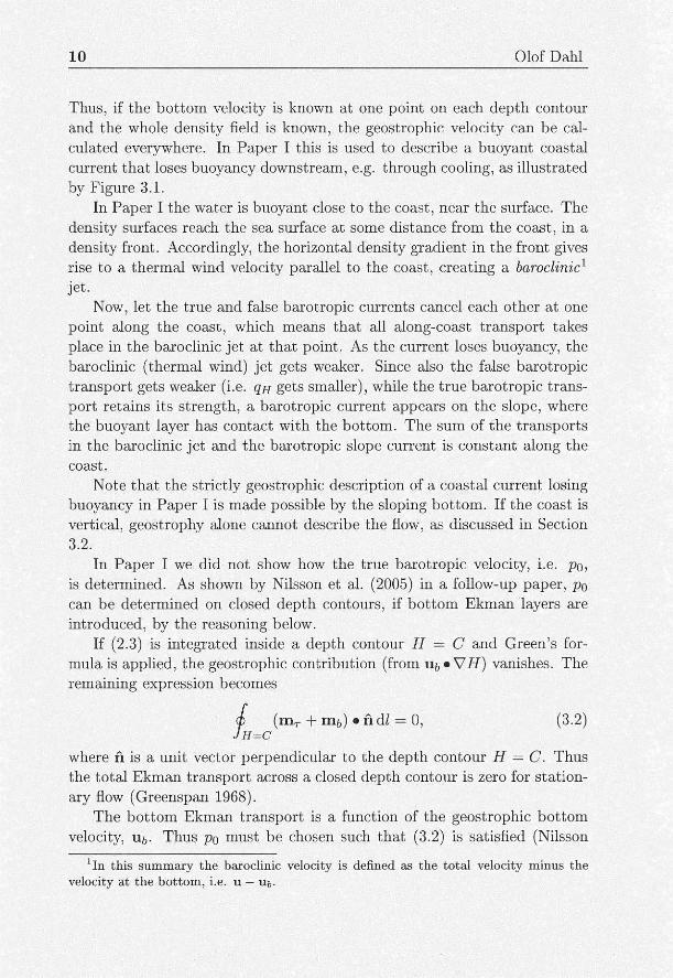
Thus, if t he bottom velocity is known at one point on each depth contour and the whole density field is known, the geostrophic velocity can be cal­culated everywhere. In Paper I this is used to describe a buoyant coastal current that loses buoyancy downstream, e.g. through cooling, as illustrated by Figure 3.1.

In Paper I the water is buoyant close to the coast, near the surface. The density surfaces reach the sea surface at some distance from the coast, in a density front. Accordingly, the horizontal density gradient in the front gives rise to a thermal wind velocity parallel to the coast, creating a baroclinic1

jet. Now, let the true and false barotropic currents cancel each other at one

point along the coast, which means that all along-coast transport takes place in the baroclinic jet at that point. As the current loses buoyancy, the baroclinic (thermal wind) jet gets weaker. Since also the false barotropic transport gets weaker (i.e. qn gets smaller), while the true barotropic trans­port retains its strength, a barotropic current appears on the slope, where the buoyant layer has contact with the bottom. The sum of t he transports in the baroclinic jet and the barotropic slope current is constant along the coast.

Note that the strictly geostrophic description of a coastal current losing buoyancy in Paper I is made possible by the sloping bottom. If the coast is vertical, geostrophy alone cannot describe the flow, as discussed in Section 3.2.

In Paper I we did not show how the true barotropic velocity, i.e. po, is determined. As shown by Nilsson et al. (2005) in a follow-up paper, po can be determined on closed depth contours, if bottom Ekman layers are introduced, by the reasoning below.

If (2.3) is integrated inside a depth contour H — C and Green's for­mula is applied, the geostrophic contribution (from Uf,»VH) vanishes. The remaining expression becomes

® (mT + m(,)*ndl = 0, (3.2) JH=C

where n is a unit vector perpendicular to the depth contour H — C . Thus the total Ekman transport across a closed depth contour is zero for station­ary flow (Greenspan 1968).

The bottom Ekman transport is a function of the geostrophic bottom velocity, U{,. Thus po must be chosen such that (3.2) is satisfied (Nilsson

this summary the baroclinic velocity is defined as the total velocity minus the velocity at the bottom, i.e. u — ut.

Coastally trapped waves and currents 11

et al. 2005). In practise the exact value of po will be dependent on the parametrization of t he bottom Ekman transport, e.g. linear bottom stress as used in Paper III or quadratic bottom stress as used in Paper IV. N0st & Isachsen (2003) calculated the bottom velocities along f /H contours in the Arctic and Nordic Seas using the same process. Their paper also includes an account of how to handle variations in

3.1 Non-linearities and the preference for cyclonic flow

In the theory presented so far, i.e. a strict geostrophic flow, it is assumed that there actually exists a stationary solution. The theory is also linear, since the non-linear terms in the momentum equations has been ignored. In nature, buoyant coastal currents are often unstable, releasing eddies, and change with time due to variations in the forcing. In Paper I we con­ducted numerical experiments with a primitive equation model (MIT-gcm) to verify our description of the coastal current. We found that while our qualitative predictions were correct, non-geostrophic effects were also im­portant. Likewise Spall (2004) concluded that much of the cross-isobath buoyancy transport was carried by eddies.

Linear theory predicts that forcing driving a cyclonic (i.e. with the coast to the right) true barotropic flow will yield th e same absolute velocity as an equivalent anticyclonic forcing. The only difference should be in the sign of the true barotropic velocity. Non-linear effects can break the symme­try, but are hard to study analytically. In Paper IV a numerical primitive equation model (MIT-gcm) was therefore used to show differences between the response to cyclonic and anticyclonic forcing. Four different topogra­phies were used, all with closed depth contours. The experiments were barotropic with wind forcing and bottom friction. For each topography two experiments were conducted, one with cyclonic and one with anticyclonic forcing. The forcing was applied in the form of wind-stress parallel to the depth contours, in an area close to the eastern coast (i.e. the right hand side of th e basins in Figure 3.2). In the same spirit as Paper III, discussed in Chapter 4.1, the forcing was only present over a small portion of each contour.

The differences between the cyclonic and anticyclonic cases can be sum­marized as:

• The cyclonic experiments yielded stationary flow in accordance with

12 Olof Dahl

Cyclonic Anticyclonic

! 7.5

200 400 xaxis (km)

600 0 200 400 xaxis (km)

-12.5

-17.5

Figure 3.2: The sea surfa ce height in cm from the DBSLOPE experiments in Paper

IV. With north defined as upwards in the figure, the forcing is applied close to the

eastern coast. The bottom slope is steep in the northwest and southwest. The

anticyclonic along-slope current is weaker than the cyclonic one.

linear theory. In the anticyclonic experiments, on the other hand, topographic waves were continuously generated.

• In the cyclonic experiments, the sea surface sunk to a low level in the whole central part of the basin. In the anticyclonic experiments the corresponding sea level rise was smaller, with a large sea level rise close to the forcing region.

• In the cyclonic experiments, the flow far from the forcing, i.e. in the southern end of th e basin, was substantially stronger than in the anticyclonic experiments.

The differences between the cyclonic and anticyclonic experiments were greater for topographies where the bottom slope changed along the coast. In Figure 3.2 the sea surface height is shown for the cyclonic and anticy­clonic experiments, using a topography where the bottom slope gets steep in northwest and southwest (with north defined as upwards in Figure 3.2).

Coastally trapped waves and currents 13

3.2 Consequences of a flat bottom and vertical side walls

Over a flat bottom, the dynamics of th e flow are substantially different, as shown in numerical experiments by e.g. Winton (1997) and Spall (2004). Since Vff = 0, the topographic steering provided by (2.3) vanishes; away from the coast the geostrophic flow no longer has any preferred direction. The velocity distribution will e ither be determined from the Ekman layer parts of the continuity equation (2.3), or one has to include either non-linear effects or time dependency.

At the vertical wall, problems arise when along-coast density variations are imposed. This is easily seen if we study a two layer ocean with no motion in the lower layer. Let the upper layer vanish at some point away from the coast. Then the along-coast volume transport M in the upper layer is given by

M = (3-3)

where D is the thickness of the upper layer at the coast (Stommel 1966). If the buoyancy weakens along the coast, the layer must deepen to maintain the transport. As demonstrated in Paper I and above, no such deepening is required on a sloping boundary. Furthermore, since the flow through the wall is zero, a viscous boundary layer (or some other ageostrophic effect) is required to balance the thermal wind transport into the wall.

There are also differences in the length scales available in flat bottom and sloping bottom oceans, as demonstrated in Paper III. The main cross­current length scale over a flat bottom is the Rossby radius of deformation, \/gH/f. Over a sloping bottom the length scale of th e topographic varia­tions (generally much smaller than the Rossby radius) is more important. Since the geostrophic velocity is approximately inversely proportional to the cross-current length scale, we expect faster barotropic currents over sloping topography than over flat topography.

4 Time dependency in coastal currents

In this chapter some aspects of th e temporal variability in coastal currents, relevant to Paper II and III, are discussed. Trying to cover the whole field of temporal variations is too big a task for this thesis; for a thorough review of coa stal processes see Huthnance (1995). The reader should observe that equations presented in Chapter 2 do not describe time-dependent motion.

4.1 Establishment of a coastal current

In Paper III we study the establishment of a coastal current along a sloping coast, bordering a large flat-bottom ocean, from a state of rest. We consider barotropic flow, or the true barotropic part of a current driven by horizontal buoyancy variations. Forcing is applied through divergent Ekman layers; either surface Ekman layers generated by wind, or bottom Ekman layers generated by false barotropic flow induced by the stratification. Paper III differs from many spin-up studies (e.g. Greenspan 1968) in that the forcing is only applied over a small part of the ocean, close to the coast. This way the effects of a spatially varying forcing are easily identified. We find that the response to steady forcing can be divided into the following three parts:

(a) A stationary circulation. The velocity and pressure associated with this part can vary in both horizontal directions, but the mean pressure along a depth contour is zero.

(b) An accelerating circulation along depth contours, associated with a pressure field that is constant along each contours. This term vanishes on depth contours of infinite length.

(c) Topographic waves transmitting the response along the coast. The

Coastally trapped waves and currents 15

0.15

0.05

E 0

p- -0.05

-0.1

-0.15

-0.2 1 1 1 >— -5000 -4000 -3000 -2000 -1000 0 1000 2000 3000 4000 5000

20

15

10

5

0

-51 1 I 1 ! -5000 -4000 -3000 -2000 -1000 0 1000 2000 3000 4000 5000

y (km)

Figure 4.1: The establishment of a coastal current along sloping topography, ac­

cording to Paper III. The upper panel shows the sea surfa ce height 77 = po/gpo, the

lower di)/dx, which is approximately proportional to the along-coast velocity. Forcing

is applied in an area close t o y = 0, and the waves travel to the right. Note that

different wave modes dominate in the different panels. The figure is modi fied from Paper III.

wave field is determined from the initial condition, i.e. the requirement that the ocean is initially motionless.

The wave part (c) of the solution cancels the stationary part (a) as well as the accelerating circulation (b) until waves starting in the forcing area arrive. For each turn these waves take around the basin, the current gets stronger. If f riction is present the waves die out after some time, and the acceleration stops. In Figure 4.1 the s ea surface height rj = po/gpo (upper panel) and its cross-contour derivative d-q/dx (lower panel) is shown along one depth contour. Each line corresponds to a different time, starting from an initially flat sea surface, with the waves travelling to the right in the figure. Note that drj/dx is approximately proportional to the along-

16 Olof Dahl

slope velocity. The forcing is applied in the region near y — 0 (the coast runs along the y axis) and bottom friction is neglected. Because different wave modes have different contributions to -q and dq/dx, the development with time looks different. While the fastest mode (which goes several turns around the basin in Figure 4.1) has a considerable contribution to tj, its contribution to dt]/dx is negligible. The next fastest wave mode dominates in (h]/dx. and has travelled about halfway around the basin at the time

showed by the last line in the figure. We believe that this treatment of the establishing of a coastal current can

yield new physical insights compared to other studies (e.g. Gill & Schumann 1974), with the splitting of the solution into the three parts described above, and the inclusion of closed depth contours.

4.2 Perturbations on baroclinic currents

In Paper II the structure and propagation of small perturbations on coastal currents are investigated. This is done to gain insight into how a local change, e.g. in the wind forcing, affects the current downstream.

The coastal current used in Paper II consists of a buoyant upper layer of homogenous density overlying a motionless denser layer. (This is commonly called all/2 -layer model.) The coast is a straight vertical wall. At some distance from the coast the upper layer vanishes, forming a density front. The unperturbed current has no variations along the coast, and is in strict geostrophic balance. The perturbations have a long along-coast length scale compared to the width of the current, but can otherwise have a general shape.

Analytical solutions are obtained for perturbations on two different basic states: In the first case the unperturbed upper layer has a triangular cross-section, i.e. the velocity is constant across the current. In the second case the upper layer has shear, but constant potential vorticity. For both cases the development of an arbitrary shaped initial perturbation can be described as consisting of the following three parts:

• A coastally trapped wave. This wave has a structure much like the internal Kelvin wave, and travels with the speed of the internal Kelvin wave plus the speed of the current at the coast.

• A front ally trapped wave. This wave moves significantly slower than the current itself, and can become almost stationary in the constant

potential vorticity case.

Coastally trapped waves and currents 17

• A structure essentially advected by the current. In the first case this consists of an infinite set of wave modes . In the second case (constant potential vorticity), the structure cannot be split into wave modes, but is smeared out by the sheared current.

The conclusion is that the structure of the perturbation is important to the velocity of its spreading, depending on which of the three parts are triggered.

The literature on small perturbations on buoyant coastal currents is mas­sive, but unlike in Paper II most other works have been aimed at deriving stability properties rather than investigating the structure of the perturba­tions. Ivubokawa & Hanawa (1984), examined perturbations on a constant potential vorticity current, but did not take the third part of t he solution into account. The stability of coast al currents similar to the ones in Paper II was investigated by Killworth & Stern (1982). Their conclusion was that the current becomes unstable if the velocity is zero or reversed (i.e. flow with the coast to the left) at the coast. Paper II is limited to stable cases.

5 Future outlook

Despite the large amount of research that has been done concerning coastal currents, many questions remain unanswered. This chapter describes some possible extensions of the problems discussed in this thesis.

It would be interesting to try to build a stationary ocean model based on (2.1), determining po from the Ekman transport across closed contours, as described in Chapter 3 and by Nilsson et al. (2005). To include realistic buoyancy forcing, one would need to introduce mixing and advection of the buoyancy field, and iterate until the advection is compensated by the buoyancy sources. Building such a model for closed depth contours, or closed f/H contours, should be feasible. However, inclusion of the equator would require large additions to the theory, since the f/H contours merge as one approaches the equator.

To my knowledge no perturbation study has covered a coastal current including both a density front and a sloping bottom. Studies including sloping bottoms normally assume horizontal density surfaces, and often have a vertical coast (e.g. Allen 1975). The addition of a sloping coast would require large modifications of the theory from Paper II, but would simulate conditions in nature more closely.

In Paper III we allow forcing through bottom Ekman transports caused by false barotropic flow. The generated true barotropic current would ob­viously change the density field through advection; an effect we have ne­glected. A modification of the approach used in Paper III, including the ad­vection of density, would make it possible to model buoyant density plumes along sloping bottoms. Such a study could be a useful supplement to the scaling theories of Chapman & Lentz (1994) and Lentz & Helfrich (2002).

It is of some importance to identify the cause of t he difference between cyclonic and anti-cyclonic circulation in Paper IV. At the end of t he paper it is suggested that carefully crafted forcing can be used to examine the role of topographic waves. How to identify other possible causes of the difference is not clear at the moment.

Acknowledgments

This thesis would not have been possible without the support from my supervisor Gösta Walin. Throughout the years, Gösta has provided advice, encouragement, and stern words whenever I needed them. He has been very generous with his time, and has been a challenging discussion partner as well as a good friend both within and outside science.

I am grateful to my assistant supervisor Göran Broström for his wit and advice, to Johan Nilsson for encouragement and to Anna Wåhlin for her undying enthusiasm. All three provided invaluable support over the course of my research.

In the final stages of writing this thesis everyone has rushed to help me whenever I needed. Special thanks to Göran Björk, who kindly provided the data used in Figure 1.2, and to Signild Nerheim, who read and commented on the manuscript.

I wish to thank all staff and students at the Department of Oceanogra­phy for their help and for creating an open and generous atmosphere. Some colleagues deserves individual mention: Martin, who shared my office for four years (not an easy task!) and kept me in shape physically; Kai, who took even the most outlandish math questions seriously; Signild, who kept me sane, and initiated the musical efforts and Agneta H., who always fought for us doctoral students.

There has also been distractions (of the good kind). The leaders and scouts in Mölndals Scoutkår has let me focus on the here and now, by dragging me outdoors on hikes and camps. The Tuesday gaming group has let me escape reality. Thanks to my co-conspirator Kristofer, for providing a creative outlet. The House of Cards crew, especially the GMs Ginger and Michael, also deserves mention, for letting the Swedish guy play, and for proving that internet friendships are real.

My family provides me with much of my confidence. Although I do not need it often, I know that Berit and Ingolf will always back me up. My siblings have through the years proven to also be my best friends. I thank

20 Olof Dahl

Alexander and Teresia for bringing their older brother down to Earth when he needs it, and Einar for showing that even the tiniest nerd can be powered by long hair.

Finally I wish to thank Josefin for making me so very happy.

This thesis work has been funded by the Faculty of Science at Göteborg University.

A Notation

V - Horizontal gradient operator, i.e

J - Jacobian, i.e. J(F,G) = F x G y — F y G x

u = ( u , v ) - Horizontal velocity in the ( x , y ) direction

U5 - u at the bottom

U - Horizontal transport

w - Vertical velocity (positive upwards)

p - Pressure

po - Pressure associated with the true barotropic velocity

H - Ocean depth

n - Unit vector, normal to a depth contour

p - Seawater density

po - Reference seawater density

q - Density anomaly, defined as p = (1 — q ) p o

qn - Density anomaly at the bottom

/ - Coriolis parameter

g - Acceleration of gra vity

k - Vertical unity vector, directed upwards

mr - Wind driven Ekman transport

22 Olof Dahl

rri5 - Bottom Ekman transport

i] - Sea surface elevation

M - Along-coast surface layer transport

D - Surface layer thickness at the coast

Bibliography

Allen, J. S. (1975), 'Coastal trapped waves in a stratified ocean', Journal of Physical Oceanography 5, 300-325.

Chapman, D. C. & Lentz, S. J. (1994), 'Trapping of a coastal density front by the bottom boundary layer', Journal of Physical Ocean ography 24, 1464-1479.

Csanady, G. T. (1985), '"Pycnobathic" currents over the upper continental slope', Journal of Physical Oceanography 15, 306-315.

Ekman, V. W. (1905), 'On the influence of t he earth's rotation on ocean-currents', Arkiv för Matematik, Astronomi och F ysik 2(11), 1-52.

Gill, A. E. k, Schumann, E. H. (1974), 'The generation of long shelf waves by the wind', Journal of Physical Oceanography 2, 83-90.

Greenspan, H. P. (1968), The Theory of Rotating Fluids, first edn, Cam­bridge University Press.

Huthnance, J. M. (1984), 'Slope currents and "JEBAR"', Journal of P hys­ical Oceanography 14, 795-810.

Huthnance, J. M. (1995), 'Circulation, exchange and water masses at the ocean margin: the role of physical processes at the shelf edge.', Progress in Oceanography 35, 353-431.

Killworth, P. D. & Stern, M. E. (1982), 'Instabilities on density-driven boundary currents and fronts', Geophysical and Astrophysical Fluid Dynamics 22(1-2), 1-28.

Kubokawa, A. k Hanawa, K. (1984), 'A theory of sem igeostrophic gravity waves and its applications to the intrusion of a density current along a coast. Part 1. Semigeostrophic gravity waves', Journal of the Oceano-graphical So ciety of Japan 40, 247-259.

24 Olof Dahl

Lentz, S. J. k Helfrich, K. R. (2002), 'Buoyant gravity currents along a slop­ing bottom in a rotating fluid', Journal of Fluid Mechanics 464, 251-278.

Mertz, G. & Wright, D. G. (1992), 'Interpretations of the JEBAR term', Journal of Physical Oceanography 22, 301-305.

Nerheim, S. & Stigebrandt, A. (2006), 'On the influence of buoyancy fluxes on wind drift currents', Journal of Physical Oceanography (In press).

Nilsson, J., Walin, G. k, Broström, G. (2005), 'Thermohaline circulation induced by bottom friction in sloping-boundary basins', Journal of Marine Research 63, 705-728.

N0st, O. A. & Isachsen, P. E. (2003), 'The large-scale time-mean ocean cir­culation in the Nordic Seas and Arctic Ocean estimated from simplified dynamics', Journal of Marine Research 61(2), 175-210.

Rudels, B., Björk, G., Nilsson, J., Winsor, P., Lake, I. k Nohr, C. (2005), 'The interaction between water from the Arctic Ocean and the Nordic Seas north of Fram Strait and along the East Greenland Current: some results from the Arctic 0cean-02 expedition', Journal of Marine Sys­tems (1-2), 1-30.

Spall, M. A. (2004), 'Boundary currents and watermass transformation in marginal seas', Journal of Physical Oceanography 34, 1197-1213.

Stommel, H. (1966), The Gulf Strea m, second edn, University of Cal ifornia Press.

Walin, G. (1972), 'On the hydrographie response to transient meteorological disturbances', Tellus 24(3), 1-18.

Winton, M. (1997), 'The damping effect of b ottom topography on internal decadal-scale oscillations of th e thermohaline circulation', Journal of Physical Oceanography 27, 203-208.

På grund av upphovsrättsliga skäl kan vissa ingående delarbeten ej publiceras här. För en fullständig lista av ingående delarbeten, se avhandlingens början.

Due to copyright law limitations, certain papers may not be published here.For a complete list of papers, see the beginning of the dissertation.

Earth Sciences Centre, Göteborg University, A

1. Tengberg, A. 1995. Desertification in northern Bukina Faso and central Tunisia.

2. Némethy, S. 1995. Molecular paleontological studies of shelled marine organisms and mammal bones.

3. Söderström, M. 1995. Geoinformation in agricultural planning and advisory work.

4. Haamer, J. 1995. Phycotoxin and oceanographic studies in the development of the Swedish mussel farming industry.

5. Lundberg, L. 1995. Some aspects of volume transports and carbon fluxes in the northern North Atlantic.

6. Lång, L-O. 1995. Geological influences upon soil and groundwater acidification in southwestern Sweden.

7. Naidu, P.D. 1995. High-resolution studies of Asian quater­nary monsoon climate and carbonate records from the equatorial Indian Ocean.

8. Mattsson, J. 1996. Oceanographic studies of transports and oxygen conditions in the Öresund.

9. Årebäck, H. 1995. The Hakefjorden complex. 10. Plink, P. 1995. A sedimentologic and sequence strati-

graphic approach to ice-marginal deltas, Swedish West Coast.

11. Lundqvist, L. 1996. 1.4 Ga mafic-felsic magmatism in southern Sweden.

12. Kling, J. 1996. Sorted circles and polygons in northern Sweden.

13. Lindblad, K. 1997. Near-source behavior of the Faroe Bank Channel deep-water plume.

14. Carlsson, M. 1997. Sea level and salinity variations in the Baltic Sea,

15. Berglund, J. 1997. Mid-proterozoic evolution in south­western Sweden.

16. Engdahl, M. 1997. Clast lithology, provenance and weathering of quaternary deposits in Västergötland, Sweden.

17. Tullborg, E-L. 1997. Recognition of low-temperature processes in the Fennoscandian shield.

18. Ekman, S. 1997. Quaternary pollen biostratigraphy in the British sector of the central North Sea.

19. Broström, G. 1997. Interaction between mixed layer dyna­mics, gas exchange and biological production the oceanic surface layer with applications to the northern North Atlantic.

20. Stenvall, O. 1997. Stable isotopic (813C, 5I80) records through the Maastrichtian at Hemmor, NW Germany.

21. Loorents, K-J. 1997. Petrology, brittle structures and prospecting methods in the "Offerdalsskiffer" from the central part of the Caledonian allochton in the county of Jämtland, Sweden.

22. Lindkvist, L. 1997. Investigations of local climate variability in a mountainous area.

23. Gustafsson, B. 1997. Dynamics of the seas and straits between the Baltic and the North Seas.

24. Marek, R. 1997. The Hakefjord fault. 25. Cederbom, C. 1997. Fission track thermochronology

applied to phanerozoic thermotectonic events in central and southern Sweden.

26. Kucera, M. 1997. Quantitative studies of morphological evolution and biogeographic patterns in Cretaceous and Tertiary foraminifera.

27. Andersson, T. 1997. Late Quaternary stratigraphie and morphologic investigations in the poolepynten area, Prins Karls Forland, western Svalbard.

28. Wallinder, K. 1998. An integrated geophysical approach to the evaluation of quaternary stratigraphy and bedrock morphology in deep, sediment-filled valleys, south-west Sweden

29. Lepland, A. 1998. Sedimentary processes related to detrital and authigenic mineralogy of holocene sediments: Skagerrak and Baltic Sea.

30. Eilola, K. 1998. Oceanographic studies of the dynamics of freshwater, oxygen and nutrients in the Baltic Sea.

31. Klingberg, F. 1998. Foraminiferal stratigraphy and palaeo-environmental conditions during late Pleistocene and Holocene in south-western Sweden.

32. Charisi, S. 1998. Chemical paleoceanographic studies of the eastern Mediterranean-Middle East and eastern North Atlantic regions in the early Paleogene and late Quaternary.

33. Plink Björklund, P. 1998. Sedimentary processes and se­quence stratigraphy in Late Weichselian ice-marginal clastic bodies, Swedish west coast and in Eocene foreland basin fill, the Central Tertiary Basin, Spitsbergen.

34. Borne, K. 1998. Observational study of sea and landbreeze on the Swedish West Coast with focus on an archipelago.

35. Andersson, M. 1998. Probing crustal structures in south­western Scandinavia: Constraints from deep seismic and gravity observations.

36. Nicolescu, S. 1998. Scam genesis at Ocna de Fier-Dognecea, south-west Romania.

37. Bäckström, D. L. 1998. Late Quarternary paleoceano­graphic and paleoclimatic records from south-west of the Faeroe Islands, north-eastern Atlantic ocean.

38. Gustafsson, M. 1999. Marine aerosols in southern Sweden. 39. Haeger-Eugensson, M. 1999. Atmospheric stability and the

interaction with local and meso-scale wind systems in an urban area.

40. Engström, L. 1999. Sedimentology of recent sediments from the Göta Älv estuary-Göteborg harbour, sw Sweden.

41. Pizarro, O. 1999. Low frequency fluctuations in the Eastern Boundary Current of South America: Remote and local forcing.

42. Karlsson, M. 1999. Local and micro climatological studies with emphasis on temperature variations and road slipperiness.

43. Upmanis, H. 1999. Influence of parks on local climate. 44. Andreasson, F. 1999. Gastropod intrashell chemical

profiles (§l80, 813C, Mg/Ca, Sr/Ca) as indicators of Paleogene and recent environmental and climatic conditions.

45. Andersson, T. 1999. Late Quaternary palaeoenvironmental history of Prins Karls Forland, western Svalbard: glacia­tions, sea levels and climate.

46. Brack, K. 1999. Characterisation of facies and their relation to Holocene and recent sediment accumulation in the Göta älv estuary and archipelago.

Earth Sciences Centre, Göteborg University, A 47. Gustafsson, M. 2000.- Recent and late Holocene 73.

development of the marine environment in three fjords on the Swedish west coast.

48. Loorents, K-J. 2000. Sedimentary characteristics, brittle structures and prospecting methods of the Flammet 74. Quartzite - a feldspathic metasandstone in industrial use from the Offerdal Nappe, Swedish Caledonides. 75.

49. Marek, R. 2000. Tectonic modelling of south west Scandinavia based on marine reflection seismic data. 76.

50. Norrman, J. 2000. Road climatological studies with emphasis on winter road slipperiness. 77.

51. Ostwald, M. 2000. Local protection of tropical dry natural forest, Orissa, India.

52. Postgård, U. 2000. Road climate variations related to 78. weather and topography.

53. Johansson, M. 2000. The role of tectonics, structures and etch processes for the present relief in glaciated 79. Precambrian basement rocks of S W Sweden.

54. Ovuka, M.. 2000. Effects of soil erosion on nutrient status 80. and soil productivity in the Central Highlands of Kenya.

55. Thompson, E. 2000. Paleocene chemical paleoceanography : global paleoproductivity and regional (North Sea) 81. paleoclimate.

56. Liljebladh, B. 2000. Experimental studies of some physical 82. oceanographic processes.

57. Bengtsson, H. 2000. Sediment transport, deposition and environmental interpretations in the Skagerrak and 83. northern Kattegat: grain-size distribution, mineralogy and

heavy metal content. 84. 58. Scherstén, A. 2000. Mafic intrusions in SW Sweden :

petrogenesis, geochronology, and crustal context. 59. Arneborg, L. 2000. Oceanographic studies of internal 85.

waves and diapycnal mixing. 60. Bäckström, D.L. 2000. Late Quaternary paleoceanography 86.

and paleoclimate of the North Atlantic Ocean. 61. Liungman, O. 2000. Modelling Qord circulation and

turbulent mixing. 62. Holmberg, S. 2000. Chemical and mineralogical characteri- 87.

sation of granulated wood ash. 63. Årebäck, C. 2000. Seismic stratigraphy in the east-central 88.

Kattegat Sea. 64. Claeson, D. T. 2000. Investigation of gabbroic rocks asso­

ciated with the Småland-Värmland granitoid batholith of the Transscandinavian Igneous Belt, Sweden. 89.

65. Cederbom, C. 2001. Fission track thermochronology appl­ied to Phanerozoic thermotectonic events in the Swedish part of the Baltic Shield. 90.

66. Axell, L. 2001. Turbulent mixing in the ocean with appli­cation to Baltic Sea modeling. 91.

67. Wahlin, A. 2001. The dynamics of dense currents on slo­ping topography.

68. Nyborg, M. 2001. Geological remote sensing - an approach 92. to spatial modelling.

69. Eriksson, M. 2001. Winter road climate investigations 93. using GIS.

70. Nyberg, J. 2001. Tropical North Atlantic climate variabi­lity through the last 2000 years deduced from hermatypic 94. corals and marine sediments.

71. Sahlin, T. 2001. Physical properties and durability of un- 95. treated and impregnated dimension stones of igneous, sedi­mentary, and metamorphic origin. 96.

72. Årebäck, H. 2001. Petrography, geochemistry and geo­chronology of mafic to intermediate late Sveconorwegian intrusions: the Hakefjorden Complex and Vinga intrusion, 97. SW Sweden.

Åkesson, U. 2001. Numerical description of rock texture by using image analysis and quantitative microscopy: alter­native method for the assessment of the mechanical pro­perties of rock aggregates. Winsor, P. 2002. Studies of dense shelf water, vertical stra­tification and sea ice thickness of the Arctic Ocean. Petersson, J. 2002. The genesis and subsequent evolution of episyenites in the Bohus granite, Sweden. Johansson, B.. 2002. Estimation of areal precipitation for hydrological modelling in Sweden. Lokrantz, H. 2002. Pleistocene stratigraphy, ice sheet his­tory and environmental development in the southern Kara Sea area, Arctic Russia. Johannesson, L. 2002. Sedimentology and geochemistry of recent sediments from the Göta Älv estuary - Göteborg Harbour. Svensson, M.K. 2002. Urban climate in relation to land use, planning and comfort. Gustafsson, K.E. 2002. Tidal energy losses by baroclinic wave drag and their importance for the thermohaline circulation. Turesson, A. 2002. Geophysical methods for identifying clay below sand : two case studies, SW Sweden. Holmberg, S. 2003. Sawdust combustion residues from a converted wanderrost boiler : composition, treatment, leaching properties and mineralogy. Söderkvist, J. 2003. Sensitivity and variability of the Arctic Ocean ice cover. Andersson, H.C. 2003. Effects of topography on ocean thermohaline circulation and climate variability on Baltic Sea water exchange. Hellström, C. 2003. Regional precipitation in Sweden in relation to large-scale climate. Lindquist, K.K. 2003. Studies of the temporal and spatial variability of an ice cover, the sea surface temperature, and the colour of coral using satellite-based remote sensing techniques. Thorsson, S. 2003. Climate, air quality and thermal comfort in the urban environment. Filipsson, H.L. 2003. Recent changes in the marine environment in relation to climate, hydrography, and human impact - with special reference to fjords on the Swedish west coast. Green, J.A.M. 2004. Dynamics of the upper coastal ocean with special reference to the inshore-offshore water exchange. Tingdahl, K. 2004. Semi-automated detection and extraction of seismic objects. Sultan, L. 2004. Sedimentology and detrital zircon age distribution in the Palaeoproterozoic Västervik Basin, SE Sweden. Achberger, C. 2004. Recent and future regional climate variations in Sweden in relation to large-scale climate. Witon, E. 2004. Holocene marine and freshwater diatoms from the Faeroe Islands - Taxonomy and environmental influences. Ericson, K. 2004. Landform development in granitic terrain. Åkesson, U. 2004. Microstructures in granites and marbles in relation to their durability as a construction material. Kairyte, M. 2004. Sediment processes and source interpretations using grain size and mineralogy of Lithuanian coastal sediments. Nerheim, S. 2005. Dynamics of and horizontal dispersion in the upper layers of the sea.

Earth Sciences Centre, Göteborg University, A

98. Jonsson, P. 2005. Urban climate and air quality in tropical cities.

99. Öberg, J. 2005. Investigations of the influence of physical factors on some marine ecological systems.

100. Turesson, A. 2005. Evaluation of combined geophysical methods for characterization of near-surface sediment.

101. Pontén, A. 2005. Depositional environments and processes across regressive to transgressive turnaround : examples from the Devonian Baltic Basin and the Eocene Central Basin of Spitsbergen.

102. Drake, H. 2006. Fracture fillings and red-strained wall-rock in the Simpevarp area, SE Sweden.

103. Mil-Hommens, M. 2006. Assessment of heavy metal cont­amination in three areas off the Portuguese shelf.

104. Dahl, O. H. 2006. Coastally trapped waves and currents.

mi Kompendiet, Göteborg

2006