8. analysis of variance for unbalanced two-factor … for unbalanced two-factor experiments when...
TRANSCRIPT

8. Analysis of Variance for UnbalancedTwo-Factor Experiments
Copyright c©2018 Dan Nettleton (Iowa State University) 8. Statistics 510 1 / 76

ANOVA for Unbalanced Two-Factor Experiments
When data are unbalanced, the type I ANOVA test for two-way
interactions is the same as the test for two-way interactions
discussed previously.
However, the type I ANOVA tests for individual factors are not
the tests for main effects discussed previously.
Furthermore, the type I results for individual factors depend on
the order that the factors appear in the type I ANOVA table.
Copyright c©2018 Dan Nettleton (Iowa State University) 8. Statistics 510 2 / 76

Example Unbalanced Two-Factor Experiment
An experiment was conducted to study the effect of storage timeand storage temperature on the amount of active ingredient in adrug lost during storage. A total of 16 vials of the drug, eachcontaining approximately 30 mg/mL of active ingredient, wereassigned (using a completely randomized design) to thefollowing treatments:
1 Storage for 3 months at 20◦ C2 Storage for 3 months at 30◦ C3 Storage for 6 months at 20◦ C4 Storage for 6 months at 30◦ C
Copyright c©2018 Dan Nettleton (Iowa State University) 8. Statistics 510 3 / 76

Example Unbalanced Two-Factor Experiment
6 of the 16 vials were damaged during shipment to the labwhere the active ingredient was measured. The amount of activeingredient was measured only for the 10 undamaged vials. Thetable below shows the amount of active ingredient lost duringstorage (in tenths of mg/mL) for each of the undamaged vials.
Storage TemperatureStorage Time 20◦ 30◦
3 months 3 5 11 13 15
6 months 5 6 6 7 16
Copyright c©2018 Dan Nettleton (Iowa State University) 8. Statistics 510 4 / 76

A Cell Means Model for the Data
Let yijk denote the amount of active ingredient lost from the kth
vial treated with the ith storage time and jth temperature.
Let nij denote the number of vials measured for the ith storagetime and jth temperature.
Suppose yijk = µij + εijk (i = 1, 2; j = 1, 2; k = 1, . . . , nij), whereµ11, µ12, µ21, and µ22 are unknown real-valued parameters andthe εijk terms are i.i.d. normal random variables with mean 0 andsome unknown variance σ2 > 0.
Copyright c©2018 Dan Nettleton (Iowa State University) 8. Statistics 510 5 / 76
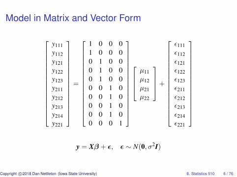
Model in Matrix and Vector Form
y111y112y121y122y123y211y212y213y214y221
=
1 0 0 01 0 0 00 1 0 00 1 0 00 1 0 00 0 1 00 0 1 00 0 1 00 0 1 00 0 0 1
µ11µ12µ21µ22
+
ε111ε112ε121ε122ε123ε211ε212ε213ε214ε221
y = Xβ + ε, ε ∼ N(0, σ2I)
Copyright c©2018 Dan Nettleton (Iowa State University) 8. Statistics 510 6 / 76
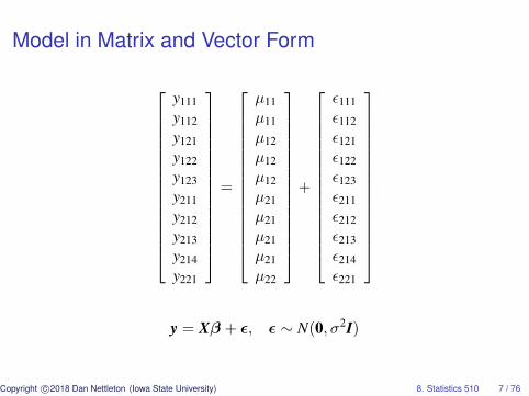
Model in Matrix and Vector Form
y111y112y121y122y123y211y212y213y214y221
=
µ11µ11µ12µ12µ12µ21µ21µ21µ21µ22
+
ε111ε112ε121ε122ε123ε211ε212ε213ε214ε221
y = Xβ + ε, ε ∼ N(0, σ2I)
Copyright c©2018 Dan Nettleton (Iowa State University) 8. Statistics 510 7 / 76

We could consider a sequence of progressively morecomplex models for the response mean that lead up toour full cell means model.
1 E(yijk) = µ
2 E(yijk) = µ+ αi
3 E(yijk) = µ+ αi + βj
4 E(yijk) = µ+ αi + βj + γij ⇐⇒ E(yijk) = µij
Copyright c©2018 Dan Nettleton (Iowa State University) 8. Statistics 510 8 / 76
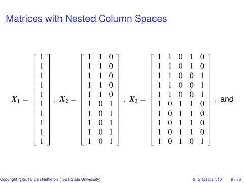
Matrices with Nested Column Spaces
X1 =
1111111111
, X2 =
1 1 01 1 01 1 01 1 01 1 01 0 11 0 11 0 11 0 11 0 1
, X3 =
1 1 0 1 01 1 0 1 01 1 0 0 11 1 0 0 11 1 0 0 11 0 1 1 01 0 1 1 01 0 1 1 01 0 1 1 01 0 1 0 1
, and
Copyright c©2018 Dan Nettleton (Iowa State University) 8. Statistics 510 9 / 76

Matrices with Nested Column Spaces
X4 =
1 0 0 01 0 0 00 1 0 00 1 0 00 1 0 00 0 1 00 0 1 00 0 1 00 0 1 00 0 0 1
Copyright c©2018 Dan Nettleton (Iowa State University) 8. Statistics 510 10 / 76

ANOVA Table
Source Sum of Squares DFTime|1 y′(P2 − P1)y 2− 1 = 1Temp|1,Time y′(P3 − P2)y 3− 2 = 1Time× Temp|1,Time,Temp y′(P4 − P3)y 4− 3 = 1Error y′(I − P4)y 10− 4 = 6C. Total y′(I − P1)y 10− 1 = 9
Copyright c©2018 Dan Nettleton (Iowa State University) 8. Statistics 510 11 / 76

The Time-Temperature Dataset
> time=factor(rep(c(3,6),each=5))> temp=factor(rep(c(20,30,20,30),c(2,3,4,1)))> a=time> b=temp> y=c(3,5,11,13,15,5,6,6,7,16)
Copyright c©2018 Dan Nettleton (Iowa State University) 8. Statistics 510 12 / 76

> d=data.frame(time,temp,y)> d
time temp y1 3 20 32 3 20 53 3 30 114 3 30 135 3 30 156 6 20 57 6 20 68 6 20 69 6 20 710 6 30 16
Copyright c©2018 Dan Nettleton (Iowa State University) 8. Statistics 510 13 / 76

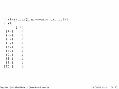
> x1=matrix(1,nrow=nrow(d),ncol=1)> x1
[,1][1,] 1[2,] 1[3,] 1[4,] 1[5,] 1[6,] 1[7,] 1[8,] 1[9,] 1
[10,] 1
Copyright c©2018 Dan Nettleton (Iowa State University) 8. Statistics 510 14 / 76

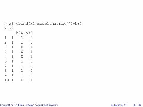
> x2=cbind(x1,model.matrix(˜0+a))> x2
a3 a61 1 1 02 1 1 03 1 1 04 1 1 05 1 1 06 1 0 17 1 0 18 1 0 19 1 0 110 1 0 1
Copyright c©2018 Dan Nettleton (Iowa State University) 8. Statistics 510 15 / 76

> x3=cbind(x2,model.matrix(˜0+b))> x3
a3 a6 b20 b301 1 1 0 1 02 1 1 0 1 03 1 1 0 0 14 1 1 0 0 15 1 1 0 0 16 1 0 1 1 07 1 0 1 1 08 1 0 1 1 09 1 0 1 1 010 1 0 1 0 1
Copyright c©2018 Dan Nettleton (Iowa State University) 8. Statistics 510 16 / 76

> x4=model.matrix(˜0+b:a)> x4
b20:a3 b30:a3 b20:a6 b30:a61 1 0 0 02 1 0 0 03 0 1 0 04 0 1 0 05 0 1 0 06 0 0 1 07 0 0 1 08 0 0 1 09 0 0 1 010 0 0 0 1
Copyright c©2018 Dan Nettleton (Iowa State University) 8. Statistics 510 17 / 76
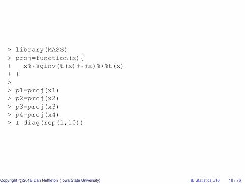
> library(MASS)> proj=function(x){+ x%*%ginv(t(x)%*%x)%*%t(x)+ }>> p1=proj(x1)> p2=proj(x2)> p3=proj(x3)> p4=proj(x4)> I=diag(rep(1,10))
Copyright c©2018 Dan Nettleton (Iowa State University) 8. Statistics 510 18 / 76

> SumOfSquares=c(+ t(y)%*%(p2-p1)%*%y,+ t(y)%*%(p3-p2)%*%y,+ t(y)%*%(p4-p3)%*%y,+ t(y)%*%(I-p4)%*%y,+ t(y)%*%(I-p1)%*%y)>> Source=c(+ "Time|1",+ "Temp|1,Time",+ "Time x Temp|1,Time,Temp",+ "Error",+ "C. Total")
Copyright c©2018 Dan Nettleton (Iowa State University) 8. Statistics 510 19 / 76

> data.frame(Source,SumOfSquares)Source SumOfSquares
1 Time|1 4.902 Temp|1,Time 176.723 Time x Temp|1,Time,Temp 0.484 Error 12.005 C. Total 194.10> anova(lm(y˜time+temp+time:temp,data=d))Analysis of Variance Table
Response: yDf Sum Sq Mean Sq F value Pr(>F)
time 1 4.90 4.90 2.45 0.1686temp 1 176.72 176.72 88.36 8.233e-05 ***time:temp 1 0.48 0.48 0.24 0.6416Residuals 6 12.00 2.00---Signif. codes: 0 *** 0.001 ** 0.01 * 0.05 . 0.1 1
Copyright c©2018 Dan Nettleton (Iowa State University) 8. Statistics 510 20 / 76

What do the F-tests in this ANOVA table test?
Recall the null hypothesis for Fj is true if and only if
β′X′(Pj+1 − Pj)Xβ = 0.
We have the following equivalent conditions
β′X′(Pj+1 − Pj)Xβ = 0 ⇐⇒ β′X′(Pj+1 − Pj)′(Pj+1 − Pj)Xβ = 0
⇐⇒ || (Pj+1 − Pj)Xβ ||2= 0⇐⇒ (Pj+1 − Pj)Xβ = 0⇐⇒ Cβ = 0,
where C is any full-row-rank matrix with the same row space as(Pj+1 − Pj)X.
Copyright c©2018 Dan Nettleton (Iowa State University) 8. Statistics 510 21 / 76
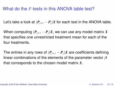
What do the F-tests in this ANOVA table test?
Let’s take a look at (Pj+1 − Pj)X for each test in the ANOVA table.
When computing (Pj+1 − Pj)X, we can use any model matrix Xthat specifies one unrestricted treatment mean for each of thefour treatments.
The entries in any rows of (Pj+1 − Pj)X are coefficients defininglinear combinations of the elements of the parameter vector βthat corresponds to the chosen model matrix X.
Copyright c©2018 Dan Nettleton (Iowa State University) 8. Statistics 510 22 / 76

Our Choice for X and β
X =
1 0 0 01 0 0 00 1 0 00 1 0 00 1 0 00 0 1 00 0 1 00 0 1 00 0 1 00 0 0 1
β =
µ11µ12µ21µ22
Copyright c©2018 Dan Nettleton (Iowa State University) 8. Statistics 510 23 / 76
Time|1 ANOVA Test
> x=x4> fractions((p2-p1)%*%x)
b20:a3 b30:a3 b20:a6 b30:a61 1/5 3/10 -2/5 -1/102 1/5 3/10 -2/5 -1/103 1/5 3/10 -2/5 -1/104 1/5 3/10 -2/5 -1/105 1/5 3/10 -2/5 -1/106 -1/5 -3/10 2/5 1/107 -1/5 -3/10 2/5 1/108 -1/5 -3/10 2/5 1/109 -1/5 -3/10 2/5 1/1010 -1/5 -3/10 2/5 1/10
> fractions(2*(p2-p1)%*%x)[1,]b20:a3 b30:a3 b20:a6 b30:a6
2/5 3/5 -4/5 -1/5
Copyright c©2018 Dan Nettleton (Iowa State University) 8. Statistics 510 24 / 76

Time|1 ANOVA Test
(P2 − P1)Xβ = 0⇐⇒ Cβ = 0,
where
Cβ =
[25
35− 4
5− 1
5
]µ11
µ12
µ21
µ22
=
(25µ11 +
35µ12
)−(
45µ21 +
15µ22
).
Copyright c©2018 Dan Nettleton (Iowa State University) 8. Statistics 510 25 / 76

Time|1 ANOVA Test 6= Time Main Effect Test
Null for Time|1 ANOVA test:
25µ11 +
35µ12 =
45µ21 +
15µ22
Null for Time main effect test:
12µ11 +
12µ12 =
12µ21 +
12µ22
i.e.µ̄1· = µ̄2·
Copyright c©2018 Dan Nettleton (Iowa State University) 8. Statistics 510 26 / 76
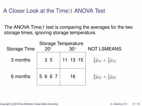
A Closer Look at the Time|1 ANOVA Test
The ANOVA Time|1 test is comparing the averages for the twostorage times, ignoring storage temperature.
Storage TemperatureStorage Time 20◦ 30◦ NOT LSMEANS
3 months 3 5 11 13 15 25 µ̂11 + 3
5 µ̂12
6 months 5 6 6 7 16 45 µ̂21 + 1
5 µ̂22
Copyright c©2018 Dan Nettleton (Iowa State University) 8. Statistics 510 27 / 76

A Closer Look at the Time|1 ANOVA Test
The ANOVA Time|1 test is comparing the averages for the twostorage times, ignoring storage temperature.
Storage TemperatureStorage Time 20◦ 30◦ NOT LSMEANS
3 months 3 5 11 13 15 25
(3+5
2
)+ 3
5
(11+13+15
3
)6 months 5 6 6 7 16 4
5
(5+6+6+7
4
)+ 1
5
(161
)
Copyright c©2018 Dan Nettleton (Iowa State University) 8. Statistics 510 28 / 76

A Closer Look at the Time|1 ANOVA Test
The ANOVA Time|1 test is comparing the averages for the twostorage times, ignoring storage temperature.
Storage TemperatureStorage Time 20◦ 30◦ NOT LSMEANS
3 months 3 5 11 13 15(
3+5+11+13+155
)= 9.4
6 months 5 6 6 7 16(
5+6+6+7+165
)= 8.0
Copyright c©2018 Dan Nettleton (Iowa State University) 8. Statistics 510 29 / 76

The Test for Time Main Effects
The test for time main effects is based on LSMEANS.
Storage TemperatureStorage Time 20◦ 30◦ LSMEANS
3 months 3 5 11 13 15 12 µ̂11 + 1
2 µ̂12
6 months 5 6 6 7 16 12 µ̂21 + 1
2 µ̂22
Copyright c©2018 Dan Nettleton (Iowa State University) 8. Statistics 510 30 / 76

The Test for Time Main Effects
The test for time main effects is based on LSMEANS.
Storage TemperatureStorage Time 20◦ 30◦ LSMEANS
3 months 3 5 11 13 15 12
(3+5
2
)+ 1
2
(11+13+15
3
)6 months 5 6 6 7 16 1
2
(5+6+6+7
4
)+ 1
2
(161
)
Copyright c©2018 Dan Nettleton (Iowa State University) 8. Statistics 510 31 / 76
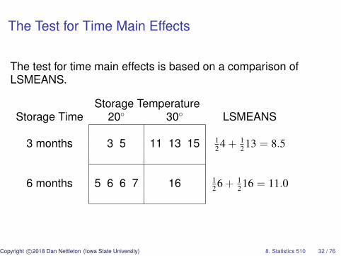
The Test for Time Main Effects
The test for time main effects is based on a comparison ofLSMEANS.
Storage TemperatureStorage Time 20◦ 30◦ LSMEANS
3 months 3 5 11 13 15 124 + 1
213 = 8.5
6 months 5 6 6 7 16 126 + 1
216 = 11.0
Copyright c©2018 Dan Nettleton (Iowa State University) 8. Statistics 510 32 / 76

Temp|1,Time ANOVA Test
> fractions((p3-p2)%*%x)b20:a3 b30:a3 b20:a6 b30:a6
1 9/25 -9/25 6/25 -6/252 9/25 -9/25 6/25 -6/253 -6/25 6/25 -4/25 4/254 -6/25 6/25 -4/25 4/255 -6/25 6/25 -4/25 4/256 3/25 -3/25 2/25 -2/257 3/25 -3/25 2/25 -2/258 3/25 -3/25 2/25 -2/259 3/25 -3/25 2/25 -2/2510 -12/25 12/25 -8/25 8/25
> fractions((25/15)*(p3-p2)%*%x)[1,]b20:a3 b30:a3 b20:a6 b30:a6
3/5 -3/5 2/5 -2/5
Copyright c©2018 Dan Nettleton (Iowa State University) 8. Statistics 510 33 / 76

Temp|1,Time ANOVA Test
(P3 − P2)Xβ = 0⇐⇒ Cβ = 0,
where
Cβ =
[35− 3
525− 2
5
]µ11
µ12
µ21
µ22
=
(35µ11 +
25µ21
)−(
35µ12 +
25µ22
).
This is not the test for a storage temperature main effect.
Copyright c©2018 Dan Nettleton (Iowa State University) 8. Statistics 510 34 / 76

Time×Temp|1,Time,Temp ANOVA Test
> fractions((p4-p3)%*%x)b20:a3 b30:a3 b20:a6 b30:a6
1 6/25 -6/25 -6/25 6/252 6/25 -6/25 -6/25 6/253 -4/25 4/25 4/25 -4/254 -4/25 4/25 4/25 -4/255 -4/25 4/25 4/25 -4/256 -3/25 3/25 3/25 -3/257 -3/25 3/25 3/25 -3/258 -3/25 3/25 3/25 -3/259 -3/25 3/25 3/25 -3/2510 12/25 -12/25 -12/25 12/25
> fractions((25/6)*(p4-p3)%*%x)[1,]b20:a3 b30:a3 b20:a6 b30:a6
1 -1 -1 1
Copyright c©2018 Dan Nettleton (Iowa State University) 8. Statistics 510 35 / 76

Time×Temp|1,Time,Temp ANOVA Test
(P4 − P3)Xβ = 0⇐⇒ Cβ = 0,
where
Cβ = [1 − 1 − 1 1]
µ11
µ12
µ21
µ22
= µ11 − µ12 − µ21 + µ22.
This is the test for Time × Temp interaction.
Copyright c©2018 Dan Nettleton (Iowa State University) 8. Statistics 510 36 / 76

We could consider a different sequence ofprogressively more complex models for the responsemean that lead up to our full cell means model.
1 E(yijk) = µ
2 E(yijk) = µ+ βj
3 E(yijk) = µ+ αi + βj
4 E(yijk) = µ+ αi + βj + γij ⇐⇒ E(yijk) = µij
Copyright c©2018 Dan Nettleton (Iowa State University) 8. Statistics 510 37 / 76
> x1=matrix(1,nrow=nrow(d),ncol=1)> x1
[,1][1,] 1[2,] 1[3,] 1[4,] 1[5,] 1[6,] 1[7,] 1[8,] 1[9,] 1
[10,] 1
Copyright c©2018 Dan Nettleton (Iowa State University) 8. Statistics 510 38 / 76
> x2=cbind(x1,model.matrix(˜0+b))> x2
b20 b301 1 1 02 1 1 03 1 0 14 1 0 15 1 0 16 1 1 07 1 1 08 1 1 09 1 1 010 1 0 1
Copyright c©2018 Dan Nettleton (Iowa State University) 8. Statistics 510 39 / 76

> x3=cbind(x2,model.matrix(˜0+a))> x3
b20 b30 a3 a61 1 1 0 1 02 1 1 0 1 03 1 0 1 1 04 1 0 1 1 05 1 0 1 1 06 1 1 0 0 17 1 1 0 0 18 1 1 0 0 19 1 1 0 0 110 1 0 1 0 1
Copyright c©2018 Dan Nettleton (Iowa State University) 8. Statistics 510 40 / 76

> x4=model.matrix(˜0+b:a)> x4
b20:a3 b30:a3 b20:a6 b30:a61 1 0 0 02 1 0 0 03 0 1 0 04 0 1 0 05 0 1 0 06 0 0 1 07 0 0 1 08 0 0 1 09 0 0 1 010 0 0 0 1
Copyright c©2018 Dan Nettleton (Iowa State University) 8. Statistics 510 41 / 76

> library(MASS)> proj=function(x){+ x%*%ginv(t(x)%*%x)%*%t(x)+ }>> p1=proj(x1)> p2=proj(x2)> p3=proj(x3)> p4=proj(x4)> I=diag(rep(1,10))
Copyright c©2018 Dan Nettleton (Iowa State University) 8. Statistics 510 42 / 76
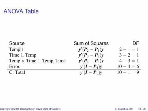
ANOVA Table
Source Sum of Squares DFTemp|1 y′(P2 − P1)y 2− 1 = 1Time|1,Temp y′(P3 − P2)y 3− 2 = 1Temp× Time|1,Temp,Time y′(P4 − P3)y 4− 3 = 1Error y′(I − P4)y 10− 4 = 6C. Total y′(I − P1)y 10− 1 = 9
Copyright c©2018 Dan Nettleton (Iowa State University) 8. Statistics 510 43 / 76

> SumOfSquares=c(+ t(y)%*%(p2-p1)%*%y,+ t(y)%*%(p3-p2)%*%y,+ t(y)%*%(p4-p3)%*%y,+ t(y)%*%(I-p4)%*%y,+ t(y)%*%(I-p1)%*%y)>> Source=c(+ "Temp|1",+ "Time|1,Temp",+ "Temp x Time|1,Temp,Time",+ "Error",+ "C. Total")
Copyright c©2018 Dan Nettleton (Iowa State University) 8. Statistics 510 44 / 76

> data.frame(Source,SumOfSquares)Source SumOfSquares
1 Temp|1 170.016672 Time|1,Temp 11.603333 Temp x Time|1,Temp,Time 0.480004 Error 12.000005 C. Total 194.10000>> anova(lm(y˜temp+time+temp:time,data=d))
Analysis of Variance Table
Response: yDf Sum Sq Mean Sq F value Pr(>F)
temp 1 170.017 170.017 85.0083 9.185e-05 ***time 1 11.603 11.603 5.8017 0.05267 .temp:time 1 0.480 0.480 0.2400 0.64160Residuals 6 12.000 2.000---Signif. codes: 0 *** 0.001 ** 0.01 * 0.05 . 0.1 1
Copyright c©2018 Dan Nettleton (Iowa State University) 8. Statistics 510 45 / 76
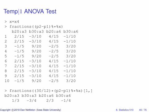
Temp|1 ANOVA Test
> x=x4> fractions((p2-p1)%*%x)
b20:a3 b30:a3 b20:a6 b30:a61 2/15 -3/10 4/15 -1/102 2/15 -3/10 4/15 -1/103 -1/5 9/20 -2/5 3/204 -1/5 9/20 -2/5 3/205 -1/5 9/20 -2/5 3/206 2/15 -3/10 4/15 -1/107 2/15 -3/10 4/15 -1/108 2/15 -3/10 4/15 -1/109 2/15 -3/10 4/15 -1/1010 -1/5 9/20 -2/5 3/20
> fractions((30/12)*(p2-p1)%*%x)[1,]b20:a3 b30:a3 b20:a6 b30:a6
1/3 -3/4 2/3 -1/4
Copyright c©2018 Dan Nettleton (Iowa State University) 8. Statistics 510 46 / 76

Temp|1 ANOVA Test
(P2 − P1)Xβ = 0⇐⇒ Cβ = 0,
where
Cβ =
[13− 3
423− 1
4
]µ11
µ12
µ21
µ22
=
(13µ11 +
23µ21
)−(
34µ12 +
14µ22
).
Copyright c©2018 Dan Nettleton (Iowa State University) 8. Statistics 510 47 / 76

Time|1,Temp ANOVA Test
> fractions((p3-p2)%*%x)b20:a3 b30:a3 b20:a6 b30:a6
1 32/75 6/25 -32/75 -6/252 32/75 6/25 -32/75 -6/253 4/25 9/100 -4/25 -9/1004 4/25 9/100 -4/25 -9/1005 4/25 9/100 -4/25 -9/1006 -16/75 -3/25 16/75 3/257 -16/75 -3/25 16/75 3/258 -16/75 -3/25 16/75 3/259 -16/75 -3/25 16/75 3/2510 -12/25 -27/100 12/25 27/100
> fractions((3/2)*(p3-p2)%*%x)[1,]b20:a3 b30:a3 b20:a6 b30:a616/25 9/25 -16/25 -9/25
Copyright c©2018 Dan Nettleton (Iowa State University) 8. Statistics 510 48 / 76
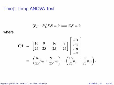
Time|1,Temp ANOVA Test
(P3 − P2)Xβ = 0⇐⇒ Cβ = 0,
where
Cβ =
[1625
925− 16
25− 9
25
]µ11
µ12
µ21
µ22
=
(1625µ11 +
925µ12
)−(
1625µ21 +
925µ22
).
Copyright c©2018 Dan Nettleton (Iowa State University) 8. Statistics 510 49 / 76

Temp×Time|1,Temp,Time ANOVA Test
> fractions((p4-p3)%*%x)b20:a3 b30:a3 b20:a6 b30:a6
1 6/25 -6/25 -6/25 6/252 6/25 -6/25 -6/25 6/253 -4/25 4/25 4/25 -4/254 -4/25 4/25 4/25 -4/255 -4/25 4/25 4/25 -4/256 -3/25 3/25 3/25 -3/257 -3/25 3/25 3/25 -3/258 -3/25 3/25 3/25 -3/259 -3/25 3/25 3/25 -3/2510 12/25 -12/25 -12/25 12/25
> fractions((25/6)*(p4-p3)%*%x)[1,]b20:a3 b30:a3 b20:a6 b30:a6
1 -1 -1 1
Copyright c©2018 Dan Nettleton (Iowa State University) 8. Statistics 510 50 / 76

Temp×Time|1,Temp,Time ANOVA Test
(P4 − P3)Xβ = 0⇐⇒ Cβ = 0,
where
Cβ = [1 − 1 − 1 1]
µ11
µ12
µ21
µ22
= µ11 − µ12 − µ21 + µ22.
Copyright c©2018 Dan Nettleton (Iowa State University) 8. Statistics 510 51 / 76
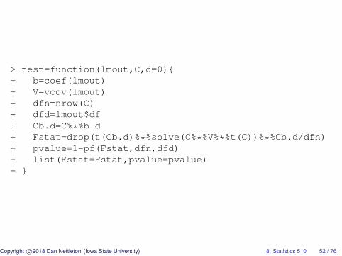
> test=function(lmout,C,d=0){+ b=coef(lmout)+ V=vcov(lmout)+ dfn=nrow(C)+ dfd=lmout$df+ Cb.d=C%*%b-d+ Fstat=drop(t(Cb.d)%*%solve(C%*%V%*%t(C))%*%Cb.d/dfn)+ pvalue=1-pf(Fstat,dfn,dfd)+ list(Fstat=Fstat,pvalue=pvalue)+ }
Copyright c©2018 Dan Nettleton (Iowa State University) 8. Statistics 510 52 / 76
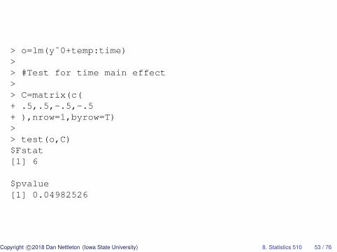
> o=lm(y˜0+temp:time)>> #Test for time main effect>> C=matrix(c(+ .5,.5,-.5,-.5+ ),nrow=1,byrow=T)>> test(o,C)$Fstat[1] 6
$pvalue[1] 0.04982526
Copyright c©2018 Dan Nettleton (Iowa State University) 8. Statistics 510 53 / 76
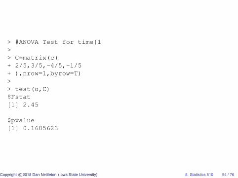
> #ANOVA Test for time|1>> C=matrix(c(+ 2/5,3/5,-4/5,-1/5+ ),nrow=1,byrow=T)>> test(o,C)$Fstat[1] 2.45
$pvalue[1] 0.1685623
Copyright c©2018 Dan Nettleton (Iowa State University) 8. Statistics 510 54 / 76
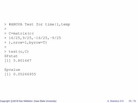
> #ANOVA Test for time|1,temp>> C=matrix(c(+ 16/25,9/25,-16/25,-9/25+ ),nrow=1,byrow=T)>> test(o,C)$Fstat[1] 5.801667
$pvalue[1] 0.05266955
Copyright c©2018 Dan Nettleton (Iowa State University) 8. Statistics 510 55 / 76
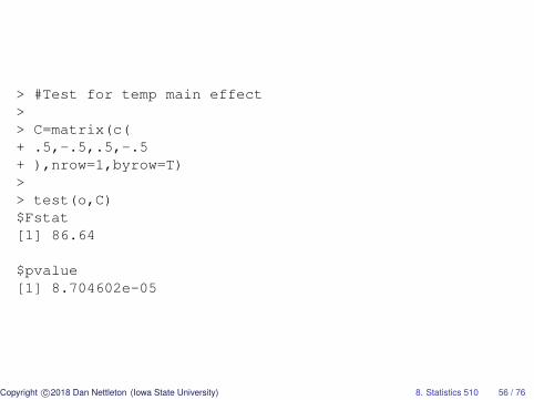
> #Test for temp main effect>> C=matrix(c(+ .5,-.5,.5,-.5+ ),nrow=1,byrow=T)>> test(o,C)$Fstat[1] 86.64
$pvalue[1] 8.704602e-05
Copyright c©2018 Dan Nettleton (Iowa State University) 8. Statistics 510 56 / 76

> #ANOVA Test for temp|1>> C=matrix(c(+ 1/3,-3/4,2/3,-1/4+ ),nrow=1,byrow=T)>> test(o,C)$Fstat[1] 85.00833
$pvalue[1] 9.185462e-05
Copyright c©2018 Dan Nettleton (Iowa State University) 8. Statistics 510 57 / 76

> #ANOVA Test for temp|1,time>> C=matrix(c(+ 3/5,-3/5,2/5,-2/5+ ),nrow=1,byrow=T)>> test(o,C)$Fstat[1] 88.36
$pvalue[1] 8.233372e-05
Copyright c©2018 Dan Nettleton (Iowa State University) 8. Statistics 510 58 / 76
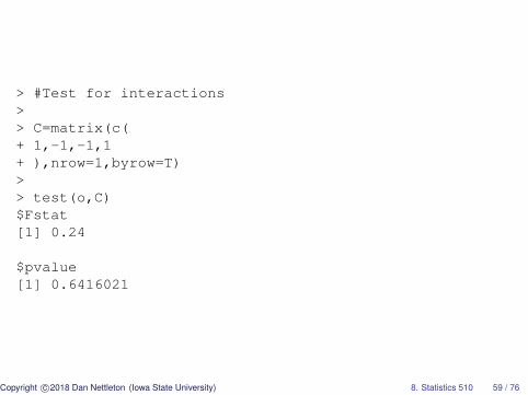
> #Test for interactions>> C=matrix(c(+ 1,-1,-1,1+ ),nrow=1,byrow=T)>> test(o,C)$Fstat[1] 0.24
$pvalue[1] 0.6416021
Copyright c©2018 Dan Nettleton (Iowa State University) 8. Statistics 510 59 / 76

Different Types of Sums of Squares
Source Type I Type II Type III
A SS(A|1) SS(A|1,B) SS(A|1,B,AB)
B SS(B|1,A) SS(B|1,A) SS(B|1,A,AB)
AB SS(AB|1,A,B) SS(AB|1,A,B) SS(AB|1,A,B)
Error SSE SSE SSE
C. Total SSTotal ? ?
Copyright c©2018 Dan Nettleton (Iowa State University) 8. Statistics 510 60 / 76
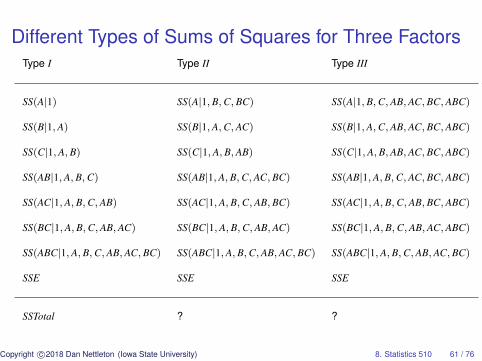
Different Types of Sums of Squares for Three FactorsType I Type II Type III
SS(A|1) SS(A|1,B,C,BC) SS(A|1,B,C,AB,AC,BC,ABC)
SS(B|1,A) SS(B|1,A,C,AC) SS(B|1,A,C,AB,AC,BC,ABC)
SS(C|1,A,B) SS(C|1,A,B,AB) SS(C|1,A,B,AB,AC,BC,ABC)
SS(AB|1,A,B,C) SS(AB|1,A,B,C,AC,BC) SS(AB|1,A,B,C,AC,BC,ABC)
SS(AC|1,A,B,C,AB) SS(AC|1,A,B,C,AB,BC) SS(AC|1,A,B,C,AB,BC,ABC)
SS(BC|1,A,B,C,AB,AC) SS(BC|1,A,B,C,AB,AC) SS(BC|1,A,B,C,AB,AC,ABC)
SS(ABC|1,A,B,C,AB,AC,BC) SS(ABC|1,A,B,C,AB,AC,BC) SS(ABC|1,A,B,C,AB,AC,BC)
SSE SSE SSE
SSTotal ? ?
Copyright c©2018 Dan Nettleton (Iowa State University) 8. Statistics 510 61 / 76

Sums of Squares for Balanced Data
For balanced data, the three types of sums of squares areidentical: Type I=Type II=Type III.
This equality in not obvious (at least to most normal humans),but it is true. We will not attempt to prove this in 510.
The ANOVA F tests in the ANOVA table can be used to test forfactor main effects and interactions.
Copyright c©2018 Dan Nettleton (Iowa State University) 8. Statistics 510 62 / 76
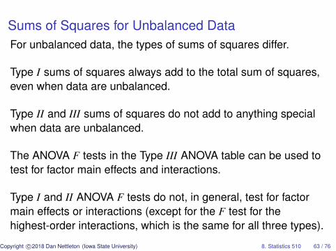
Sums of Squares for Unbalanced DataFor unbalanced data, the types of sums of squares differ.
Type I sums of squares always add to the total sum of squares,even when data are unbalanced.
Type II and III sums of squares do not add to anything specialwhen data are unbalanced.
The ANOVA F tests in the Type III ANOVA table can be used totest for factor main effects and interactions.
Type I and II ANOVA F tests do not, in general, test for factormain effects or interactions (except for the F test for thehighest-order interactions, which is the same for all three types).
Copyright c©2018 Dan Nettleton (Iowa State University) 8. Statistics 510 63 / 76
SAS Code and Output
proc glm;class time temp;model y=time temp time*temp / ss1 ss2 ss3;
run;
The GLM Procedure
Class Level Information
Class Levels Valuestime 2 3 6temp 2 20 30
Number of Observations Read 10Number of Observations Used 10
Copyright c©2018 Dan Nettleton (Iowa State University) 8. Statistics 510 64 / 76

Dependent Variable: y
Sum ofSource DF Squares Mean Square F Value Pr > F
Model 3 182.1000000 60.7000000 30.35 0.0005
Error 6 12.0000000 2.0000000
Corrected Total 9 194.1000000
R-Square Coeff Var Root MSE y Mean
0.938176 16.25533 1.414214 8.700000
Copyright c©2018 Dan Nettleton (Iowa State University) 8. Statistics 510 65 / 76

Source DF Type I SS Mean Square F Value Pr > F
time 1 4.9000000 4.9000000 2.45 0.1686temp 1 176.7200000 176.7200000 88.36 <.0001time*temp 1 0.4800000 0.4800000 0.24 0.6416
Source DF Type II SS Mean Square F Value Pr > F
time 1 11.6033333 11.6033333 5.80 0.0527temp 1 176.7200000 176.7200000 88.36 <.0001time*temp 1 0.4800000 0.4800000 0.24 0.6416
Source DF Type III SS Mean Square F Value Pr > F
time 1 12.0000000 12.0000000 6.00 0.0498temp 1 173.2800000 173.2800000 86.64 <.0001time*temp 1 0.4800000 0.4800000 0.24 0.6416
Copyright c©2018 Dan Nettleton (Iowa State University) 8. Statistics 510 66 / 76

Type IV Sums of Squares
In addition to computing Type I, II, and III sums of squares, SAScan compute Type IV sums of squares.
Type IV sums of squares are only relevant for factorial designswith missing cells.
When cells are missing, I recommend determining the linearcombinations of the estimable cell means that are of scientificinterest, and then conducting the corresponding tests as tests ofH0 : Cβ = d.
Copyright c©2018 Dan Nettleton (Iowa State University) 8. Statistics 510 67 / 76

Calculation of Type I, II, and III Sums of Squares
Every Type I, II, or III sum of squares is the error sums ofsquares for a reduced model minus the error sum of squares fora model that adds one term to the reduced model:
y′(I − PXreduced)y− y′(I − PXreduced+term)y = y′(PXreduced+term − PXreduced)y,
where C(Xreduced) ⊂ C(Xreduced+term) ⊆ C(X).
As usual, X represents the model matrix for the most complexmodel under consideration (a.k.a., the full model).
For all Type III sums of squares, the reduced+term model is thefull model.
Copyright c©2018 Dan Nettleton (Iowa State University) 8. Statistics 510 68 / 76
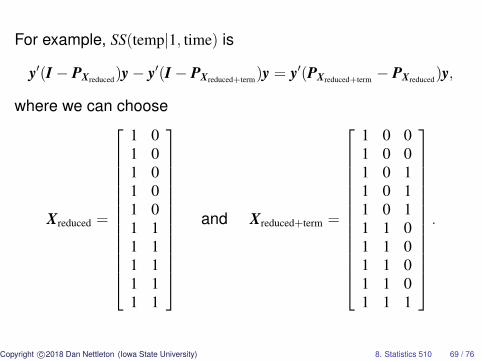
For example, SS(temp|1, time) is
y′(I − PXreduced)y− y′(I − PXreduced+term)y = y′(PXreduced+term − PXreduced)y,
where we can choose
Xreduced =
1 01 01 01 01 01 11 11 11 11 1
and Xreduced+term =
1 0 01 0 01 0 11 0 11 0 11 1 01 1 01 1 01 1 01 1 1
.
Copyright c©2018 Dan Nettleton (Iowa State University) 8. Statistics 510 69 / 76

How does this apply to a Type III Sum of Squares likeSS(time|1, temp, time× temp)?
Here the reduced+term model is actually the full cell meansmodel that includes an intercept, time and temperature maineffects, and time × temperature interaction.
The reduced model has an intercept, temperature main effect,and time × temperature interaction but no time main effect.
How do we fit such a reduced model?
Copyright c©2018 Dan Nettleton (Iowa State University) 8. Statistics 510 70 / 76
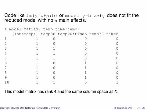
Code like lm(y˜b+a:b) or model y=b a*b; does not fit thereduced model with no a main effects.
> model.matrix(˜temp+time:temp)(Intercept) temp30 temp20:time6 temp30:time6
1 1 0 0 02 1 0 0 03 1 1 0 04 1 1 0 05 1 1 0 06 1 0 1 07 1 0 1 08 1 0 1 09 1 0 1 010 1 1 0 1
This model matrix has rank 4 and the same column space as X.
Copyright c©2018 Dan Nettleton (Iowa State University) 8. Statistics 510 71 / 76

Removing Time Main Effect from Cell Means Model
TempTime 20◦ 30◦ Marginal Mean
3 months µ11 µ12 µ̄1· = (µ11 + µ12)/2
6 months µ21 µ22 µ̄2· = (µ21 + µ22)/2
The parameters µ11, µ12, µ21, and µ22 can be anything as long as
µ̄1· = µ̄2· ⇐⇒ µ22 = µ11 + µ12 − µ21.
Copyright c©2018 Dan Nettleton (Iowa State University) 8. Statistics 510 72 / 76
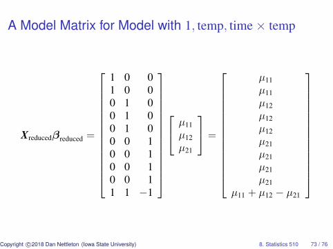
A Model Matrix for Model with 1, temp, time× temp
Xreducedβreduced =
1 0 01 0 00 1 00 1 00 1 00 0 10 0 10 0 10 0 11 1 −1
µ11
µ12
µ21
=
µ11
µ11
µ12
µ12
µ12
µ21
µ21
µ21
µ21
µ11 + µ12 − µ21
Copyright c©2018 Dan Nettleton (Iowa State University) 8. Statistics 510 73 / 76

#Type III Sum of Squares for SS(time|1,temp,time x temp)> x0=x[,1:3]> x0[10,]=c(1,1,-1)> x01 1 0 02 1 0 03 0 1 04 0 1 05 0 1 06 0 0 17 0 0 18 0 0 19 0 0 110 1 1 -1> anova(lm(y˜0+x0),lm(y˜0+x))Analysis of Variance TableModel 1: y ˜ 0 + x0Model 2: y ˜ 0 + xRes.Df RSS Df Sum of Sq F Pr(>F)
1 7 242 6 12 1 12 6 0.04983 *
Copyright c©2018 Dan Nettleton (Iowa State University) 8. Statistics 510 74 / 76
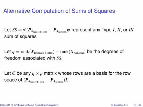
Alternative Computation of Sums of Squares
Let SS = y′(PXreduced+term − PXreduced)y represent any Type I, II, or IIIsum of squares.
Let q = rank(Xreduced+term)− rank(Xreduced) be the degrees offreedom associated with SS.
Let C be any q× p matrix whose rows are a basis for the rowspace of (PXreduced+term − PXreduced)X.
Copyright c©2018 Dan Nettleton (Iowa State University) 8. Statistics 510 75 / 76

Alternative Computation of Sums of Squares
Then the ANOVA F statistic
SS/qMSE
=β̂′C′[C(X′X)−C′]−1Cβ̂/q
σ̂2 .
Thus, any SS can be computed as β̂′C′[C(X′X)−C′]−1Cβ̂ for an
appropriate matrix C.
Copyright c©2018 Dan Nettleton (Iowa State University) 8. Statistics 510 76 / 76