DOI: 10.24427/978-83-66391-87-1_08

87

Mykhaylo ANDRIYCHUK1, Uliana MARIKUTSA2

8. MODELING MATERIALS WITH

DESIRED REFRACTIVE INDEX

The explicit solution to the diffraction problem on a set of small particles, supplemented

into homogeneous material, is used for modeling the materials with the desired refractive

index. The consideration concerns to the case of acoustic scalar scattering and the solution

to initial scattering problem is built using an asymptotic approach. The closed form solution

is reduced for the scattering problem. This lets an explicit formula for the refractive index

of the resulting inhomogeneous material to be obtained. The numerical calculations show

the possibility of getting the specific values of refractive index including its negative

values.

8.1. INTRODUCTION

The materials with the specific physical properties, in particular with negative refractive

index play an important role in the process of improving the radiation performances of the

different IC and radioelectronic devices. Such materials are used widely for improving the

radiation performances of microstrip antennas of different types, microwave filters and

field transformers. There are different approaches to forming specific properties of the

medium (material) by embedding into it a series of inclusions. This leads to the formation

of the physical properties of resulting material that are different to those that are inherent

to the properties of initial material. The theoretical prediction of the existence of such

materials was made in the pioneer work [1] and thereon, such materials were designed by

the variety recipes. As early as the eighties of the last century, these materials received the

name chiral and began to be used in various areas of antenna technology [2], manufacturing

of electronic devices [3], [4], and telecommunications equipment [5]. The goal of this paper

is to propose the numerical approach (based on [6] and [7]) for modeling the material with

the specific refractive index, including its negative values. The approach foresees reducing

1 Ivan Franko National University of Lviv, Ukraine 2 Lviv Polytechnic National University, Ukraine

88

an explicit solution to the respective acoustic scattering problem, and the explicit formula

for the resulting refractive index based on the asymptotic solution to acoustic wave

scattering problem on a set of big number of embedded particles of small size. The chapter

is organized as follows: Section 8.2 is devoted to statement of diffraction problem and

outline of application limits of geometrical and physical parameters of the material under

consideration. The analytical form of solution will be derived in Section 8.3, and the

numerical aspects of solving the respective system of linear algebraic equations (SLAE)

will be presented here. The explicit formula for the refractive index of resulting

inhomogeneous material will be derived in Section 8.4. The numerical results, related to

exactness of asymptotic solution to the initial diffraction problem and properties of material

with obtained refractive index will be presented in Section 8.5. A short conclusion finalizes

the discussed topic under consideration.

8.2. STATEMENT OF SCATTERING PROBLEM

A combination of both the asymptotic method and numerical simulation is used to solve

the problem of creating a material with specified scattering characteristics, particularly,

with a given refractive index. The initial diffraction problem is solved by assumption:

𝑘𝑎 ≪ 1, and 𝑑 ≫ 𝑎, a is the characteristic size of the particle, 𝑑 is the distance between

adjacent particles, 𝑘 = 2𝜋/𝜆 is the wave number.

An asymptotic solution to the scattering problem on many particles by assumptions:

𝑑 = 𝑂(√𝑎3

), and 𝑀 = 𝑂(𝑎−1) was obtained in [6], 𝑀 is the total number of particles

contained in a given domain 𝐷 ⊂ 𝑅3.

The impedance boundary conditions

𝜁𝑚 = 𝑞(𝑥𝑚)/𝑎𝜅 (8.1)

are prescribed on the boundary 𝑆𝑚 of 𝑚-th particle, where 𝜁𝑚 is boundary impedance,

𝑥𝑚 ∈ 𝐷𝑚, 𝑞𝑚 = 𝑞(𝑥𝑚); 𝑞(𝑥) is arbitrary function, continuous in 𝐷; 𝐼𝑚 𝑞 ≤ 0, and

𝑑 = 𝑂(𝑎(2−𝜅)/3), where 𝑀 = 𝑂(1/𝑎2−𝜅), and 𝜅 ∈ (0,1).

The incident field satisfies Helmholtz equation in the whole 𝑅3, by this, the scattered

field satisfies the radiation conditions. We assume that a small particle is a sphere of radius

𝑎 with center in point xm, 1 ≤ 𝑚 ≤ 𝑀.

The full field 𝑢𝑀 satisfies equation

[∇2 + 𝑘2𝑛02(𝑥)]𝑢𝑀 = 0 in the domain 𝑅3\ ⋃ 𝐷𝑚

𝑀𝑚−1 , (8.2)

and boundary conditions

𝜕𝑢𝑀/𝜕𝑁 = 𝜁𝑚𝑢𝑀 in 𝑆𝑚, where 1 ≤ 𝑚 ≤ 𝑀, (8.3)

and

𝑢𝑀 = 𝑢0 + 𝑣𝑀 , (8.4)

89

𝑢0 is the solution of problem (8.2) – (8.4) at M=0 (namely, when 𝐷 does not contain the

particles), 𝑢0 = 𝑒𝑖𝑘𝛼⋅𝑥 is the incident field, and field 𝑣𝑀 satisfies the radiation conditions.

Let 𝑞(𝑥) belong to 𝐶(𝐷), Δ𝑝 ⊂ 𝐷 is arbitrary subdomain of 𝐷, and 𝐾(Δ𝑝) is the total

number of particles in Δ𝑝 determined by

𝐾(Δ𝑝) = 1/𝑎2−𝜅 ∫ 𝑁(𝑥)𝑑𝑥 ⋅ [1 + 𝑜(1)] at 𝑎 → 0𝛥𝑝

, (8.5)

where function 𝑁(𝑥) ≥ 0 is given and continuous in domain 𝐷.

It was substantiated in [6] that there exists some specific field 𝑢𝑒(𝑥) (limiting field),

which satisfies the next condition

𝑙𝑖𝑚𝑎→0‖𝑢𝑒(𝑥) − 𝑢(𝑥)‖ = 0, (8.6)

and solution to the initial diffraction problem (8.2) – (8.4) can be sought from the equation

𝑢(𝑥) = 𝑢0(𝑥) − 4𝜋 ∫ 𝐺(𝑥, 𝑦)𝑞(𝑦)𝑁(𝑦)𝑢(𝑦)𝑑𝑦𝐷

, (8.7)

where 𝐺(𝑥, 𝑦) is the Green function for Helmholtz equation (8.2) for the case of absence

of the particles. This fact allows us to use the approximate solution 𝑢𝑒(𝑥) instead of exact

solution 𝑢(𝑥) and to obtain an explicit formula for refractive index of constructed

inhomogeneous material.

8.3. THE SEMIANALYTICAL FORM OF SOLUTION

TO SCATTERING PROBLEM

In order to derive the explicit formula for approximate field, we introduce the concept

of limiting (effective) field 𝑢𝑒(𝑥). In paper [6], it was substantiated that the exact solution

to problem (8.2) – (8.4) can be presented in the form

𝑢𝑀(𝑥) = 𝑢0(𝑥) + ∑ ∫ 𝐺(𝑥, 𝑦)𝑆𝑚

𝑀

𝑚=1

𝜐𝑚(𝑦)𝑑𝑦. (8.8)

Despite the fact that this last equation contains an unknown function 𝜐𝑚(𝑦) in the

integrand, in contrast to formula (8.7), where all functions in the integrands are known, it

is used to obtain an approximate solution to the original diffraction problem. For this goal,

we define the effective field 𝑢𝑒(𝑥, 𝑎) = 𝑢𝑒(𝑚)

(𝑥), which acts on the m-th particle as

𝑢𝑒(𝑥) = 𝑢𝑀(𝑥) − ∫ 𝐺(𝑥, 𝑦)𝜐𝑚(𝑦)𝑑𝑦𝑆𝑚

, 𝑥 ∈ 𝑅3, (8.9)

and the next relation for the neighboring points is valid |𝑥 − 𝑥𝑚| ∼ 𝑎. We present the exact

formula (8) in form

90

𝑢𝑀(𝑥) = 𝑢0(𝑥) + ∑ 𝐺(𝑥, 𝑥𝑚)𝑅𝑚

𝑀

𝑚=1

+ ∑ ∫ [𝐺(𝑥, 𝑦) − 𝐺(𝑥, 𝑥𝑚)]𝜐𝑚(𝑦)𝑑𝑦𝑆𝑚

,

𝑀

𝑚=1

(8.10)

where the values 𝑅𝑚 are

𝑅𝑚 = ∫ 𝜐𝑚(𝑦)𝑑𝑦𝑆𝑚

. (8.11)

Using the known relation for function 𝐺(𝑥, 𝑦) from [8], and the asymptotic formula for

values 𝑅𝑚 [6], we obtain the next formula for 𝑢𝑀(𝑥)

𝑢𝑀(𝑥) = 𝑢0(𝑥) + ∑ 𝐺(𝑥, 𝑥𝑚)𝑅𝑚𝑀𝑚=1 + 𝑜(1) at 𝑎 → 0 for |𝑥 − 𝑥𝑚| ≥ 𝑎. (8.12)

The values 𝑅𝑚 are defined by the asymptotic formula

𝑅𝑚 = −4𝜋𝑞(𝑥𝑚)𝑢𝑒(𝑥𝑚)𝑎2−𝜅[1 + 𝑜(1)], if 𝑎 → 0, (8.13)

and asymptotic formula for function 𝜐𝑚 is

𝜐𝑚 = −𝑞(𝑥𝑚)𝑢𝑒(𝑥𝑚) ⋅1

𝑎𝜅⋅ [1 + 𝑜(1)], if 𝑎 → 0. (8.14)

Using last two formulas, we obtain the asymptotic representation of the effective field in

the vicinity of particles

𝑢𝑒(𝑗)

(𝑥) = 𝑢0(𝑥) − 4𝜋 ∑ 𝐺(𝑥, 𝑥𝑚)

𝑀

𝑚=1,𝑚≠𝑗

𝑞(𝑥𝑚)𝑢𝑒(𝑥𝑚)𝑎2−𝜅[1 + 𝑜(1)], (8.15)

which is valid in the domains |𝑥 − 𝑥𝑗| ≤ 𝑎,   where 1 ≤ 𝑗 ≤ 𝑀.

In order to calculate the values of the effective field everywhere using formula (8.15),

we should know the values 𝑢𝑒(𝑥𝑚). They can be easily obtained as solutions to the

following SLAE

𝑢𝑗 = 𝑢0𝑗 − 4𝜋 ∑ 𝐺(𝑥𝑗, 𝑥𝑚)

𝑀

𝑚=1,𝑚≠𝑗

𝑞(𝑥𝑚)𝑢𝑚𝑎2−𝜅 for 𝑗 = 1, . . . , 𝑀, (8.16)

where 𝑢𝑗 = 𝑢(𝑥𝑗) and 𝑗 = 1,2, … , 𝑀. The matrix of SLAE (8.16) is diagonally dominant,

therefore it is convenient for solving numerically. It was proven in [9] that this SLAE has

a unique solution for sufficiently small 𝑎.

In order to justify the exactness of solution to SLAE (8.16), which is used for

determination of the effective field, we derive different SLAE, corresponding to the

91

limiting equation (8.7). Let us divide the domain 𝐷, where the small particles are located,

into an union of the small non-intersecting cubes Δ𝑝 with centers at points 𝑦𝑝, the side of

such cubes can be chosen as 𝑂(𝑑1/2). Because the limited quantity of cubes cannot give

whole 𝐷, we consider their smallest partition that contains 𝐷, and define values 𝑛02 = 1 in

the cubes, which do not belong to domain 𝐷.

In order to find the solution to equation (8.7), we apply the collocation method proposed

in [9]. In accordance with this method, we obtain such SLAE

𝑢𝑗 = 𝑢0𝑗 − 4𝜋 ∑ 𝐺(𝑥𝑗 , 𝑥𝑝)

𝑃

𝑝=1,𝑝≠𝑗

𝑞(𝑦𝑝)𝑁(𝑦𝑝)𝑢𝑝|𝛥𝑝|, 𝑗 = 1, . . . , 𝑃 (8.17)

where 𝑃 is the number of cubes that form a partition of 𝐷, 𝑦𝑝 is a center of 𝑝-th cube, |Δ𝑝|

is its volume. Since the value of 𝑑 is small, diameter Δ𝑝 can be of an order larger than

distance 𝑑 between particles. Since 𝑃 ≪ 𝑀, then solving SLAE (8.17) is much easier that

solving SLAE (8.16) in terms of the number of calculations.

As a result, we have two different SLAE (8.16) and (8.17). Solving both the SLAE, we

can compare their solutions and evaluate the area of accuracy of asymptotic solution (8.15).

This evaluation has also a practical importance as allows the determination of the optimal

parameters of the domain 𝐷, which provide the possibility to create the refractive index

that is the closest to the desired one.

8.4. REFRACTIVE INDEX OF THE OBTAINED MATERIAL

The explicit formula (8.7) for the effective field opens the way to determining the

refractive index of the obtained material. It is important from the practical point of view,

how the calculated refractive index 𝑛𝑀2 (𝑥) differs from those obtained from the theoretical

assumptions. We confine here by the real refractive index and formulate the constructive

algorithm to obtain the desired one. It consists of three steps.

• Step 1: using known 𝑛02(𝑥) and unknown 𝑛2(𝑥), we calculate function

𝑝(𝑥) = 𝑘2[𝑛02(𝑥) − 𝑛2(𝑥)] = 𝑝1(𝑥).

• Step 2: using the relation 𝑝(𝑥) = 4𝜋𝑞(𝑥)𝑁(𝑥) we determine

𝑁(𝑥)𝑞(𝑥) =𝑝1(𝑥)

4𝜋. (8.18)

Equation (8.18) for two unknown functions 𝑞(𝑥) and 𝑁(𝑥) has infinite number of

solutions {𝑞(𝑥), 𝑁(𝑥)}, for which the conditions 𝑁(𝑥) ≥ 0 are fulfilled. In this

connection, the solution to (8.18) we determine as

𝑞(𝑥) =𝑝1(𝑥)

4𝜋𝑁. (8.19)

Calculation of 𝑁(𝑥) and 𝑞(𝑥) by (8.19) finalized Step 2 of our procedure.

• Step 3: is completely constructive and its goals are the following:

- to create on the small particle of radius 𝑎 the necessary impedance 𝑞(𝑥𝑚)/𝑎𝜅;

92

- to embed the particles that satisfies the properties (8.19) into domain with the initial

properties.

The application of the above algorithm was considered in [10] for the case of complex

function 𝑞(𝑥), the above algorithm can be applied if material is lossless.

8.5. NUMERICAL MODELING

8.5.1. Checking the applicability of asymptotic solution

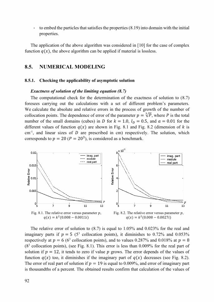
Exactness of solution of the limiting equation (8.7)

The computational check for the determination of the exactness of solution to (8.7)

foresees carrying out the calculations with a set of different problem’s parameters.

We calculate the absolute and relative errors in the process of growth of the number of

collocation points. The dependence of error of the parameter 𝑝 = √𝑃3

, where 𝑃 is the total

number of the small domains (cubes) in 𝐷 for 𝑘 = 1.0, 𝑙𝐷 = 0.5, and 𝑎 = 0.01 for the

different values of function 𝑞(𝑥) are shown in Fig. 8.1 and Fig. 8.2 (dimension of 𝑘 is

cm-1, and linear sizes of 𝐷 are prescribed in cm) respectively. The solution, which

corresponds to 𝑝 = 20 (𝑃 = 203), is considered as a benchmark.

Fig. 8.1. The relative error versus parameter 𝑝,

𝑞(𝑥) = 𝑘2(0.008 − 0.0011𝑖)

Fig. 8.2. The relative error versus parameter 𝑝,

𝑞(𝑥) = 𝑘2(0.008 − 0.0027𝑖)

The relative error of solution to (8.7) is equal to 1.05% and 0.023% for the real and

imaginary parts if 𝑝 = 5 (53 collocation points), it diminishes to 0.72% and 0.053%

respectively at 𝑝 = 6 (63 collocation points), and to values 0.287% and 0.018% at 𝑝 = 8

(83 collocation points), (see Fig. 8.1). This error is less than 0.009% for the real part of

solution if 𝑝 = 12, it tends to zero if value 𝑝 grows. The error depends of the values of

function 𝑞(𝑥) too, it diminishes if the imaginary part of 𝑞(𝑥) decreases (see Fig. 8.2).

The error of real part of solution if 𝑝 = 19 is equal to 0.009%, and error of imaginary part

is thousandths of a percent. The obtained results confirm that calculation of the values of

93

approximate field can be carried out with the high enough accuracy, and this accuracy is

attained in a wide range of the geometrical and physical parameters of the material under

investigation.

The results of computations show that the relative error depends of the parameter 𝑘 to

a large extent. In Fig. 8.3 and Fig. 8.4, the error is shown at 𝑘 = 2.5 and 𝑘 = 0.75

respectively, 𝑞(𝑥) = 𝑘2(0.008 − 0.0011𝑖). One can see that the error is of one order larger

at 𝑘 = 2.5. The maximal error (if 𝑝 = 5) at 𝑘 = 0.75 is less on 27% than those for

𝑘 = 1.0.

Fig. 8.3. The relative error versus parameter 𝑝,

𝑘 = 2.5

Fig.8.4. The relative error versus parameter 𝑝,

𝑘 = 0.75

Comparison of solutions to limiting equation (8.7) and asymptotic SLAE (8.16)

In the previous subsection, we consider the solution to SLAE (8.17) with 𝑝 = 20 as

benchmark solution to equation (8.7). The maximal value of relative error for this 𝑝 does

not exceed 0.009% for wide range of the problem’s parameters. The numerical calculations

are presented for the different sizes of 𝐷 and different functions 𝑁(𝑥). The obtained results

for small values 𝑚 are shown in Table 8.1 for 𝑙𝐷 = 1.0, 𝑘 = 1.0, and 𝑁(𝑥) = 40.

The values of 𝑎𝑒𝑠𝑡, which are received by formula (8.20), when the expected number

𝐾(Δ𝑝) of particles is changed by 𝑀. For this case, the radius of particle is determined as

𝑎𝑒𝑠𝑡 = (𝑀/ ∫ 𝑁(𝑥)𝑑𝑥𝛥𝑝

)

1/(2−𝜅)

. (8.20)

Table 8.1. The optimal parameters of domain 𝐷 at small 𝑚, 𝑁(𝑥) = 40

𝑚 8 10 12 14 16

𝑎𝑒𝑠𝑡 0.1397 0.0682 0.0378 0.0247 0.0152

𝑎𝑜𝑝𝑡 0.1054 0.0603 0.0369 0.0252 0.0169

𝑑 0.1329 0.1099 0.0917 0.0787 0.0679

Relative error 2.47% 0.42% 0.41% 1.09% 0.77%

The values of 𝑎𝑜𝑝𝑡 in the third row correspond to the optimal values of radius 𝑎, which

guarantees the minimal error for module of solution to equation (8.7) and system (8.16).

94

In the fourth row, the values of distance 𝑑 between particles are shown. The maximal value

of error is attained at 𝑚 = 8, the error diminishes if 𝑚 grows. The numerical results for

large 𝑚 with the same initial data are shown in Table 8.2. The minimal error of solution is

attained at 𝑚 = 65 (total number of particles 𝑀=27.46·104), and it is equal to 0.20%.

Table 8.2. The optimal parameters of domain 𝐷 at large 𝑚, 𝑁(𝑥) = 40

𝑚 25 35 45 55 65

𝑎𝑒𝑠𝑡 0.0079 0.0024 0.00121 6.45·10-4 3.96·10-4

𝑎𝑜𝑝𝑡 0.0076 0.0022 0.0010 6.31·10-4 3.89·10-4

𝑑 0.0514 0.0329 0.0241 0.0198 0.0171

Relative error 0.53% 0.31% 0.34% 0.23% 0.20%

Table 8.3 contains the comparable results for 𝑁(𝑥) = 4 with the same set of initial data.

One can see that the relative error diminishes if the number 𝑀 of particles increases (one

should note that the relative error depends on parameters 𝑎 and 𝑙𝐷 too). This error tends to

relative error of solution to equation (8.7) if the value of m becomes larger than 80

(𝑀 = 5.12 · 105).

Table 8.3. The optimal parameters of domain 𝐷 at large 𝑚, 𝑁(𝑥) = 4

𝑚 25 35 45 55 65

𝑎𝑒𝑠𝑡 9.98·10-4 3.30·10-4 1.51·10-4 8.19·10-5 4.99·10-5

𝑎𝑜𝑝𝑡 1.02·10-3 3.32·10-4 1.51·10-4 8.20·10-5 4.99·10-5

𝑑 0.0526 0.0345 0.0256 0.0204 0.0169

Relative error 0.19% 0.09% 0.1108% 0.06% 0.02%

Investigation of difference between solutions to SLAE (8.16) and (8.17)

The comparison of solutions to SLAE (8.16) and (8.17) was carried out for the different

values of 𝑎 at different 𝑝 and 𝑚. The relative error of SLAE (8.16) diminishes if 𝑝 increases

while 𝑚 remains constant. As an example, if p increases to 50%, then the relative error

diminishes to 11.7% (if 𝑝 = 8 and 𝑝 = 12, 𝑚 = 15).

Fig. 8.5. Dependence of deviation

of the solution’s components

of distance 𝑑 between particles, 𝑁(𝑥) = 10

Fig 8.6. Dependence of deviation

of the solution’s components

of distance 𝑑 between particles, 𝑁(𝑥) = 30

95

The differences in solutions to SLAE (8.16) and (8.17) in the real part, imaginary part,

and module are shown in Figs. 8.5 and 8.6 if 𝑝 = 7 and 𝑚 = 15. By this, the difference of

real parts do not exceed 3.9% at 𝑎 = 0.01, it is less than 3.3% at 𝑎 = 0.007, and it is less

than 1.85% if 𝑎 = 0.004, 𝑑 = 9𝑎, and 𝑁(𝑥) = 20. Respectively, this difference is less

than 0.075% if 𝑝 = 11, 𝑎 = 0.001, and 𝑁(𝑥) = 30, 𝑑 = 15𝑎 (𝑚 is the same).

The numerical results, obtained for a wide range of 𝑑, show that its optimal value exists,

and starting from this value, the deviations of solutions begin to increase again.

Such optimal values of 𝑑 are presented in Table 8.4 for the different constant 𝑁(𝑥).

The results obtained testify that the optimal distance between particles increases if the

number of particles grow. For the small number of particles, the optimal distance is of the

same order that 𝑎, for the set number of particles (𝑀 = 153, namely 𝑚 = 15). This distance

is of an order larger. The values of the minimal and maximal errors, which are attained for

the optimal 𝑑, are shown in Table 8.5.

Table 8.4. Optimal values of 𝑑 for the different constant 𝑁(𝑥)

Value of 𝑁(𝑥)

10 20 30 40 50

𝑎 = 0.004 0.0711 0.0468 0.0468 0.0469 0.0381

𝑎 = 0.01 0.0864 0.0559 0.0595 0.0594 0.0496

Table 8.5. The relative error of solution to SLAE (8.16) in % (min/max) for the optimal 𝑑

Value of 𝑁(𝑥)

10 20 30 40 50

𝑎 = 0.004 0.69/0.09 5.17/0.48 0.48/0.109 0.95/0.121 0.28/0.06

𝑎 = 0.01 2.39/0.19 1.67/0.29 0.51/0.09 2.4/0.41 1.47/0.17

The obtained results allow us to conclude that the optimal value of 𝑑 diminishes slower,

when function 𝑁(𝑥) grows, additionally this trend is more significant for the smaller 𝑎.

5.2. Modeling the material with the desired refractive index

Numerical calculations are carried out for the case 𝑁(𝑥) = 𝑐𝑜𝑛𝑠𝑡. For simplicity, we

consider the case when a given domain 𝐷 consists of the same subdomains Δ𝑝. This limit

is not essential for the numerical modeling.

Numerical calculations were performed for the case when 𝐷 = ⋃ Δ𝑝𝑃𝑝=1 , and 𝑃 = 203,

𝐷 is some cube with side 𝑙𝐷 = 0.5 and particles are placed uniformly in domain 𝐷 (the

relative error of the solution to system (8.16) does not exceed 0.01% for this 𝑃). Let the

initial domain 𝐷 be the material with the initial refractive index 𝑛02(𝑥) = 1. Then the values

𝛮(Δ𝑝) can be calculated using the formula (8.5). On the other hand, we can choose the

number 𝑚 such that 𝑀 = 𝑚3 is closest to number 𝛮(Δ𝑝). It is easy to see that the

corresponding 𝑛2(𝑥) for such 𝑀 is calculated by such formula

96

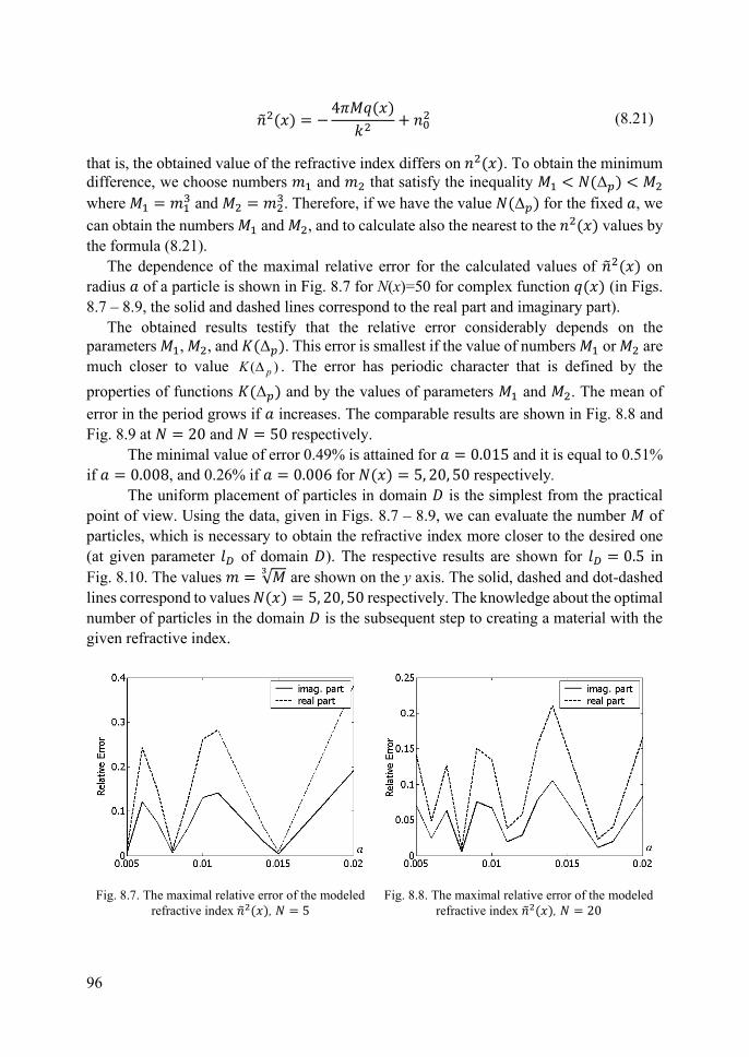
�̃�2(𝑥) = −4𝜋𝑀𝑞(𝑥)

𝑘2+ 𝑛0

2 (8.21)

that is, the obtained value of the refractive index differs on 𝑛2(𝑥). To obtain the minimum

difference, we choose numbers 𝑚1 and 𝑚2 that satisfy the inequality 𝑀1 < 𝛮(Δ𝑝) < 𝑀2

where 𝑀1 = 𝑚13 and 𝑀2 = 𝑚2

3. Therefore, if we have the value 𝛮(Δ𝑝) for the fixed 𝑎, we

can obtain the numbers 𝑀1 and 𝑀2, and to calculate also the nearest to the 𝑛2(𝑥) values by

the formula (8.21).

The dependence of the maximal relative error for the calculated values of �̃�2(𝑥) on

radius 𝑎 of a particle is shown in Fig. 8.7 for N(x)=50 for complex function 𝑞(𝑥) (in Figs.

8.7 – 8.9, the solid and dashed lines correspond to the real part and imaginary part).

The obtained results testify that the relative error considerably depends on the

parameters 𝑀1, 𝑀2, and 𝐾(Δ𝑝). This error is smallest if the value of numbers 𝑀1 or 𝑀2 are

much closer to value ( )pK . The error has periodic character that is defined by the

properties of functions 𝐾(Δ𝑝) and by the values of parameters 𝑀1 and 𝑀2. The mean of

error in the period grows if 𝑎 increases. The comparable results are shown in Fig. 8.8 and

Fig. 8.9 at 𝑁 = 20 and 𝑁 = 50 respectively.

The minimal value of error 0.49% is attained for 𝑎 = 0.015 and it is equal to 0.51%

if 𝑎 = 0.008, and 0.26% if 𝑎 = 0.006 for 𝑁(𝑥) = 5, 20, 50 respectively.

The uniform placement of particles in domain 𝐷 is the simplest from the practical

point of view. Using the data, given in Figs. 8.7 – 8.9, we can evaluate the number 𝑀 of

particles, which is necessary to obtain the refractive index more closer to the desired one

(at given parameter 𝑙𝐷 of domain 𝐷). The respective results are shown for 𝑙𝐷 = 0.5 in

Fig. 8.10. The values 𝑚 = √𝑀3

are shown on the y axis. The solid, dashed and dot-dashed

lines correspond to values 𝑁(𝑥) = 5, 20, 50 respectively. The knowledge about the optimal

number of particles in the domain 𝐷 is the subsequent step to creating a material with the

given refractive index.

Fig. 8.7. The maximal relative error of the modeled

refractive index �̃�2(𝑥), 𝑁 = 5

Fig. 8.8. The maximal relative error of the modeled

refractive index �̃�2(𝑥), 𝑁 = 20

97

The data shown in Fig. 8.10 testify that the optimal number of particles diminishes if

their radius 𝑎 grows. The estimation √𝑎(2−𝜅)3 determines the distance 𝑑 between particles.

This distance differs from that is determined by uniform placement of particles in 𝐷. As an

example, for 𝑁 = 5, 𝑎 = 0.0107 it is equal to 0.1361, and the calculated 𝑑 is equal to 0.119

and 0.159 for 𝑚 = 5 and 𝑚 = 4 respectively. The computations show that the relative

difference between these two values of 𝑑 is quite proportional to the relative error of the

refractive index.

Since this value 𝑑 does not depend on the diameter of 𝐷 in accordance to estimation

𝑑 = √𝑎(2−𝜅)3, it can be applied as an additional parameter for optimization while choosing

the alternative values of 𝑚. On the other hand, we can evaluate the number of particles in

𝐷 by the known formula [10]. With 𝐾(Δ𝑝), we can calculate the quantity 𝑀 of particles if

they are distributed uniformly in 𝐷. The distance between particles is calculated easy too

if 𝑙𝐷 is prescribed.

Fig. 8.9. The maximal relative error of the

calculated refractive index �̃�2(𝑥), 𝑁 = 50

Fig. 8.10. The optimal value of 𝑚 versus

radius 𝑎 of particles for different 𝑁(𝑥)

8.6. CONCLUSIONS

The asymptotic approach has been developed to solve the problem of acoustic scattering

on a set of small size particles (bodies) placed in a homogeneous material. The scattering

problem is reduced to solving a corresponding SLAE whose dimension is equal to the

number of particles. The solutions of this system are used in the formula of explicit

representation of the components of the scattered field. Numerical calculations are

performed that determine the accuracy of the obtained solution depending on the physical

parameters of the problem.

The obtained numerical results demonstrate the possibility of applying the proposed

technique to create materials with specified acoustic properties, in particular the refractive

index. A constructive algorithm for modeling the material with the desired refractive index

is proposed.

The results of numerical modeling open up the possibility of engineering solutions for

practical applications. As an example, uniform placement of particles is the easiest way to

98

engineering design, and the answer to how many particles should be placed in a given

domain is given by the numerical simulation results.

The engineering problems regarding the placement of a large number of small particles

in a given domain 𝐷 and creating on their surface the necessary impedance 𝜁 = 𝑞(𝑥)/𝑎𝜅

require the separate technological solutions.

REFERENCES

[1] VESELAGO V. G., The electrodynamics of substances with simultaneously negative values of ε and μ,

Soviet Physics Uspekhi, vol. 10, no 4, p. 509–514. doi:10.1070/PU1968v010n04ABEH003699, 1967.

[2] OGIER R., FANG Y. M., SVEDENDAHL M., Near-complete photon spins electivity in a metasurface

of anisotropic plasmonic antennas, Physics Reviev X, vol. 5, p. 041019, 2015.

[3] PENDRY J. B., SCHURIG D., SMITH D. R., Controlling electromagnetic fields, Science, vol. 312,

p. 1780–1782, 2006.

[4] YANG Y. et al, Circularly polarized light detection by a chiral organic semiconductor transistor, Nature

Photonics, vol. 7, p. 634–638, 2013.

[5] CHALABI H., SCHOEN D, BRONGERSMA M. L., Hot-electron photodetection with a plasmonic

nanostripe antenna, Nanotechnology Letters, vol. 14, p. 1374–1380, 2014.

[6] RAMM G., Wave scattering by many small particles embedded in a medium, Physics Letters A, vol. 372,

p. 3064-3070, 2008.

[7] RAMM A. G., Electromagnetic wave scattering by small impedance particles of an arbitrary shape,

Journal of Applied Mathematics and Computing (JAMC), vol. 43, no 1, p. 427–444, 2013.

[8] RAMM A. G., Many body wave scattering by small bodies and applications, Journal of Mathematical

Physics, vol. 48, no 10, p. 1035-1–1035-6, 2007.

[9] RAMM A. G., A Collocation method for solving integral equations, International Journal of Computing

Science and Mathematics, vol. 3, no 2, p. 122–128, 2009.

[10] ANDRIYCHUK M. I., RAMM A. G., Scattering by many small particles and creating materials with

a desired refraction coefficient, International Journal of Computing Science and Mathematics, vol. 3,

no 1/2, p. 102–121, 2010.