On the Fracture of Thin Laminates

Sharon Kao-Walter Karlskrona, 2004

Department of Mechanical Engineering School of Engineering

Blekinge Institute of Technology SE-371 79 Karlskrona, Sweden

© Sharon Kao-Walter Blekinge Institute of Technology Dissertation Series No. 2004:07 ISSN 1650-2159 ISBN 91-7295-048-X Published 2004 Printed by Kaserntryckeriet AB Karlskrona 2004 Sweden

ii

Acknowledgements

This work was carried out at the Department of Mechanical Engineering, School of Engineering, Blekinge Institute of Technology (BTH), Karlskrona, Sweden. The financial support from Tetra Pak R&D AB, Tetra Brik Carton Ambient AB, Blekinge Institute of Technology, the Swedish Knowledge Foundation (KKS) and the Print Research Program (T2F) is gratefully acknowledged. First of all, I would like to thank my supervisor, Professor Per Ståhle at the Division of Solid Mechanics at Malmö University, Malmö, Sweden, for guidance, comments and suggestions during the course of the work. I highly appreciate the valuable discussions that took my understanding of this research field to a higher level. I would like to express my appreciation to all my co-workers, especially Doctor Shaohua Chen at the Chinese Acadamy of Sciences and Licentiate Rickard Hägglund at SCA for your contributions. I wish to thank my colleagues at the Department of Mechanical Engineering at BTH and at the Division of Solid Mechanics at Malmö University for your friendly support. Thanks also to my colleagues at Tetra Pak for inspiration, for preparing the testing materials and for kindly helping me to find the relevant data. I am also grateful to my former colleagues at the Department of Solid Mechanics, Lund Institute of Technology, and especially professor Bertram Broberg for guiding me into the world of fracture mechanics and for supervising my licentiate thesis in the field of dynamic fracture mechanics. Finally, I would like to thank Professor Göran Broman, Doctor Mats Walter (BTH) and Doctor Johan Tryding (Tetra Pak) for valuable comments during the last part of the thesis work. Karlskrona, December 2004 Sharon Kao-Walter

iii

To Mats: For your encouragement that helped me to find the balance between family and career. To my lovely children Björn, Fredrik & Lisen: For giving me so much fun! To my MaMa, BaBa & my little brother: For your unlimited love and support to many of my new ideas. To the big family Walter: For all the great time we spend together. To all my friends: For your friendships that make my life even more dynamic.

iv

Abstract

This thesis concerns mechanical and fracture properties of a thin aluminium foil and polymer laminate that is widely used as packaging material. The possibility of controlling the path of the growing crack propagation by adjustment of the adhesion level and the property of the polymer layer is investigated. First, the fracture process of the aluminium foil is investigated experimentally. It is found that fracture occurs at a much lower load than what is suggested by standard handbook fracture toughness. Observations in a scanning electron microscope with a tensile stage show that small-scale stable crack growth occurs before the stress intensity factor reaches its maximum. An examination using an optical profilometric method shows almost no plastic deformation except for in a small necking region at the crack tip. However, accurate predictions of the maximum load are obtained using a strip yield model with a geometric correction. Secondly, the mechanical and fracture properties of the laminate are studied. A theory for the mechanics of the composite material is used to evaluate a series of experiments. Each of the layers forming the laminate is first tested separately. The results are analysed and compared with the test results of the entire laminate with varied adhesion. The results show that tensile strength and strain at peak stress of the laminate, with or without a crack, increase when the adhesion of the adhesive increases. It is also found that a much larger amount of energy is consumed in the laminated material at tension compare with the single layers. Possible explanations for the much higher toughness of the laminate are discussed. Finally, the behaviour of a crack in one of the layers, perpendicular to the bimaterial interface in a finite solid, is studied by formulating a dislocation superposition method. The stress field is investigated in detail and a so-called T stress effect is considered. Furthermore, the crack tip driving forces are computed numerically. The results show that the analytical methods for an asymptotically small crack extension can also be applied for a fairly large amount of crack growth. By comparing the crack tip driving force of the crack deflected into the interface with that of the crack penetrating into the polymer layer, it is shown how the path of the crack can be controlled by selecting a proper adhesion level of the interface for different material combinations of the laminate.

v

Thesis

Disposition

This thesis includes an introductory part and papers A to E. The papers have been slightly reformatted. Their content is, however, unchanged. Paper A

Kao-Walter, S. and Ståhle, P., Fracture behaviour of a thin Al-foil – measuring and modelling of the fracture processes. Submitted for publication. (Parts of the results have been published in SPIE 3rd ICEM proceeding, ISBN: 0-8194-4261-5, Wu, X., Qin, Y., Fang, J., Ke, J. (eds.), Beijing, China, 2001, 253-256.).

Paper B

Kao-Walter, S., Dahlström, J., Karlsson, T., and Magnusson, A., A study of the relation between the mechanical properties and the adhesion level in a laminated packaging material. Mech. of Comp. Mat., 2004, 40(1), 29-36 (43-52 in Russian edition). Paper C

Kao-Walter, S., Ståhle, P. and Hägglund, R., Fracture toughness of a laminated composite. Fracture of Polymers, Composites and Adhesives II, Elsevier Science, Blackman, B. R. K. Pavan, A. and Williams, J. G. (Eds.), ISBN: 0-08-044195-5, 2003, Oxford, UK, 357-364. Paper D

Chen, S. H., Wang, T. C. and Kao-Walter, S., A crack perpendicular to the bimaterial interface in finite solid. Int. J. of Solids and Structures, 2003, 40, 2731-2755.

vi

Paper E

Kao-Walter, S., Ståhle, P. and Chen, S.H., A crack penetrating or deflecting into an interface in a thin laminate. Submitted for publication. The Author’s Contribution to the Papers

The appended papers are the result of joint efforts. The present author’s contributions are as follows: Paper A

Initiated the work. Planned and carried through the experiments. Wrote the paper under the guidance of Ståhle. Paper B

Initiated the work together with Magnusson. Performed experiments together with Dahlström and Karlsson. Wrote the paper together with all authors. Paper C

Initiated the work together with Ståhle. Performed the experiments together with Hägglund. The paper was written jointly by all authors. Paper D

Initiated the work together with Chen. Took part in the calculations and discussions during the working process. Paper E

Initiated the work. Performed the finite element analysis. Wrote the paper under the guidance of Ståhle.

vii

viii

Table of Contents

1 Introduction 1 2 Fracture Behaviour of Thin Aluminium Foil 33 Mechanical and Fracture Properties of the Laminate 6 4 Behaviour of Fracture Process Region at the Interface 9 5 Conclusions 12 References 14 Appended Papers

Paper A 17 Paper B 39 Paper C 57 Paper D 73 Paper E 111

ix

x

1 Introduction

Food packages have become part of our daily life. Because of the development of packaging industries, it has become possible to buy well-stored food produced thousands of miles away. At the same time, packaging companies as well as the consumers start to pay attention to societal sustainability aspects. Using less raw materials, reducing costs and developing the functionalities of the packages have become goals for research and development. An important step is to understand the mechanical and fracture behaviour of the packaging material. Figure 1(a) shows a typical laminate structure of a packaging material used for aseptic liquid food package that may have the shelf life-time up to one year. Each of the layers contributes certain properties to the structure. The upper layer of the low-density polyethylene (LDPE) is used to protect the paperboard from direct contact with water and to avoid moist from penetrating into the paperboard, since the paperboard plays an important role for grip stiffness function of the package. A second LDPE layer is used to laminate the paperboard and an aluminium foil (Al-foil) together. The Al-foil prevents oxygen and light from reaching the food product. A last layer of the LDPE laminates together with the Al-foil by an adhesive layer, which may increase the adhesion to a desired level.

LDPE

Paperboard

LDPE

Al-foil

(a) (b)

Figure 1. (a). Components of a typical liquid food packaging material (not in scale). (b). Microscope picture of the packaging material after folding.

LDPE Adhesive

inside

1

During production, the material goes through different processes such as printing, coating, creasing, laminating, perforation etc. To become a food package, the material also needs to be formed, folded, filled, etc. Figure 1(b) shows an example of a packaging material after folding. Before reaching the consumer, the packages have to tolerate loading during transport and distribution. As the result of this loading, small cracks can often be observed in the Al-foil layer. If these cracks propagate or grow together into certain size, the barrier function of the Al-foil becomes insufficient. If one or several cracks propagate into the inside polymer layer, the shelf life of the product will be reduced. In practice, the ambition is to lead the possibbly existed cracks in the Al-foil into the interface between the Al-foil and the inside polymer layer. Thus, the large size of the cracks in the Al-foil and fracture of the interior polymer layer may be avoided. On the other hand, in the applications like the opening arrangement, the cracks in Al-foil need to be secured to go through the interface into the polymer layer. Much work has been done in the field of fracture mechanics related to packaging materials. A considerable amount of work is presented on analysis of fracture behaviours of paperboard. Many of them can be found in [1-2]. In [3-5], adhesively bounded joints have been studied through experiments and the fracture mechanics theory analysis. A review work in [6] has described the fundamental behaviour of the fracture process region at the interface of layered material. More works in the field can be found in, for example, [7-9]. This thesis will mostly investigate the fracture behaviour of the Al-foil and the LDPE laminate close to the inside of the packaging material (cf. figure 1a). Experiment and analyses of the notched and un-notched laminate specimen will be performed and solutions about the interaction of a crack and an interface in a finite solid will be discussed.

2

2 Fracture Behaviour of a Thin Aluminium Foil

Al-foil has been used in food package technology as an efficient barrier towards exposure to oxygen and light. The thickness of the foil is often only 6-10 µm. For such a thin foil the fracture toughness cannot be measured according to the ASTM standard [10]. As discussed in [11], for determination of the fracture toughness in thin plates, the measurement must be done for the actual plate thickness in the application. Therefore, tensile tests with a 15×250 mm strip and fracture toughness tests, with a centred crack panel (see figure 2(a)) and with a single edge-notched tension specimen of miniature size (see figure 2(b)), are performed. The results in paper A and B show that the mechanical properties such as Young’s modulus, strength at break and load when fracture occurs as well as the fracture toughness of the thin Al-foil are much lower as compared with standard handbook values.

σο

a0

u

L

W

a 2W

2H

2aX1

θ r X2

σο

(a) (b)

Figure 2. Geometry of the specimens. (a). Centred crack specimen with coordinate system (2W = 95 mm, 2H = 230 mm). (b) Single edge-notched

tension specimen (W= 4.5 mm, L = 8 mm).

3

For the miniature specimen shown in figure 2b, the fracture path was followed in a Scanning Electron Microscope (SEM) with a tensile stage. In the analytical part of paper A, a strip yield model [12] with the geometry correction:

⎥⎦

⎤⎢⎣

⎡⎟⎟⎠

⎞⎜⎜⎝

⎛−= 22

0

2

8exparccos2

b

c

b

c

aK

σφπ

πσσ

(1)

is found to be in good agreement with the experimental results. While the linear elastic fracture mechanics equation:

σ c

σ b=

Kc

σ b πa0φ (2)

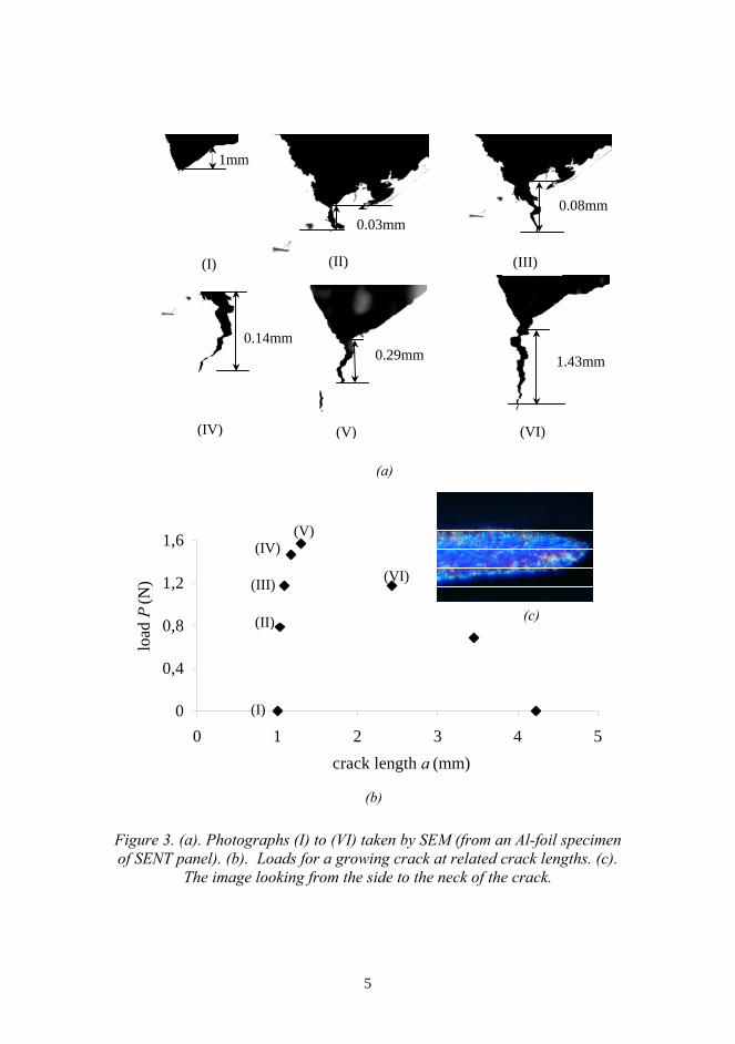
can only be used when the crack length is large (see figures 4 and 7 in paper A). In equations (1) and (2), σc is the stress at crack growth and σb is the stress at break without a pre-crack. Kc is the fracture toughness obtained from the experiments. The geometry correction, φ, can be found in, for example, [13]. This model is also assumed to be a suitable model for the other single layers in the packaging material [14]. Another important discovery is that no fracture surface can be observed using optical profilometry under the microscope as shown in figure 3c. Fracture seems to occur through so-called necking. Although stable crack growth is detected before the maximum load is reached (figure 3a and b), there are no traces of plasticity outside the crack plane.

4

1.43mm

(V)

0.29mm

0.08mm

0.14mm

0.03mm

1mm

(I)

(VI) (IV)

(III)(II)

0

0,4

0,8

1,2

1,6

0 1 2 3 4 5crack length a (mm)

load

P(N

)

(a)

(c)

(V) (IV)

(III)

(II)

(I)

(VI)

(b)

Figure 3. (a). Photographs (I) to (VI) taken by SEM (from an Al-foil specimen of SENT panel). (b). Loads for a growing crack at related crack lengths. (c).

The image looking from the side to the neck of the crack.

5

3 Mechanical and Fracture Properties of a Laminate

In many food package applications, an Al-foil is laminated with a polymer layer to act as a moisture barrier as well as to protect the liquid food product from reacting with the Al-foil. In order to understand the mechanical behaviours of this laminate, tensile tests are performed for an Al-foil/LDPE laminate with different adhesion levels. All together five different specimens are prepared: a single layer of Al-foil (Case 1), a single layer of LDPE (Case 2), Al-foil laminated by LDPE with an adhesive layer (Case 3), Al-foil laminated by LDPE without an adhesive layer (Case 4) and a case that put together Al-foil and LDPE (Case 5). The results in paper B show that Young’s modulus can be accurately calculated by the theory of the elastic mechanics of composite materials as [15]:

( ) ⎟⎟⎠

⎞⎜⎜⎝

⎛

−

⎟⎟⎠

⎞⎜⎜⎝

⎛

−−⎟

⎟⎠

⎞⎜⎜⎝

⎛

−=

∑∑

∑∑

2

2

2

2

2

1

11

i

iii

i

iii

i

ii

LtEt

tEtE

E

ν

νν

ν. (3)

Here, Ei, νi and ti are Young’s modulus, Poisson's ratio and the thickness of layer i, respectively. Paper B shows that by laminating a LDPE layer on the Al-foil (Case 4), the peak stress in the Al-foil at rupture will increase from 60 MPa to 75 MPa. At the same time, the strain at peak stress increases from 1.1% to 2.2%. Further, by laminating the LDPE and the Al-foil with an additional adhesive layer (Case 3), the adhesion of the laminate will increase. The peak stress in the Al-foil at rupture will now increase more and reach 86 MPa and the strain at peak stress will increase to 4.6%. During the experiment, delamination in the laminate is found for Cases 3 and 4. It is also observed that, in some of the specimens, several small cracks appeared before the loading stress reaches the ultimate value for the laminate with the adhesive layer (Case 3). To explain this, a more detailed study is made in paper C by applying a fracture mechanical theory. In paper C, the fracture toughness of an Al-foil that is laminated by the LDPE (Case 4) and the Al-foil put together with LDPE(Case 5) as well as single layers of the Al-foil (Cases 1) and of the LDPE (Case 2) are measured for a

6

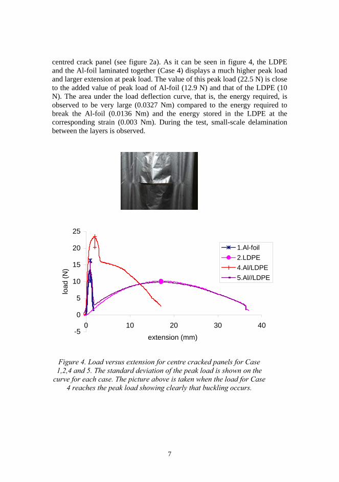
centred crack panel (see figure 2a). As it can be seen in figure 4, the LDPE and the Al-foil laminated together (Case 4) displays a much higher peak load and larger extension at peak load. The value of this peak load (22.5 N) is close to the added value of peak load of Al-foil (12.9 N) and that of the LDPE (10 N). The area under the load deflection curve, that is, the energy required, is observed to be very large (0.0327 Nm) compared to the energy required to break the Al-foil (0.0136 Nm) and the energy stored in the LDPE at the corresponding strain (0.003 Nm). During the test, small-scale delamination between the layers is observed.

-5

0

5

10

15

20

25

0 10 20 30 4

extension (mm)

load

(N)

0

1.Al-foil2.LDPE4.Al/LDPE5.Al//LDPE

Figure 4. Load versus extension for centre cracked panels for Case 1,2,4 and 5. The standard deviation of the peak load is shown on the

curve for each case. The picture above is taken when the load for Case 4 reaches the peak load showing clearly that buckling occurs.

7

Figure 4 also shows that a much larger amount of energy is consumed in the laminated material at tension. The reason for this could be that the extension of the LDPE requires multiple fracture of the Al-foil or delamination. Multiple fracture of the Al-foil would consume a large amount of energy. For Cases 4 and 5, almost the same total energy is consumed at complete fracture irrespectively of the layers are laminated together or not. Here, the energy required to break in Case 5 is equal to 0.238 Nm and 0.247 Nm in Case 4. The almost equal energies in Cases 4 and 5 rule out the hypothesis of presence of additional dissipative processes in the laminate as an explanation for the much higher toughness of the laminate. One observes also that more energy is consumed at small strains. Further, as mentioned previously, the peak load for the laminate is almost the same as the sum of the peak load for the Al-foil and the peak load for the LDPE layer. This suggests that the fracture processes distribute strain so that peak load occurs simultaneously in both materials. The assumption is that both materials reach peak stress in a small process region in the vicinity of the crack tip. It is believed that less energy is consumed during the fracture of the LDPE in the laminated case because the straining of the LDPE is concentrated to the thin gap that is defined by the broken Al-foil. The energy for onset of fracture in the Al-foil (0.0063 Nm) is certainly consumed already when the laminate has reached its peak load. This can be compared with the energy for onset of fracture in the Al-foil and the LDPE laminated together (0.0327 Nm). Unexpectedly, also the energy to break the laminate is almost entirely consumed at small straining of the specimen. The reason for this has to be sought in the mechanics of the fracture process region.

8

4 Behaviours of the Fracture Process Region at the Interface

On a small scale, the fracture process region can, possibly, be described as a crack perpendicular to a bimaterial interface in a finite solid (see figure 5). This is studied in paper D. The specimen thicknesses h1 and h2 added together equal the thickness of the laminate. The complete solutions of the problem are obtained by employing a dislocation superposition method. During the calculations, a pair of complex potentials for finite solid is developed. The influence of the loading cases, material parameters and geometries are also considered in this paper. The results show that, as the crack approaches the interface, the parameter b becomes an important length scale. This characterizes the dominated zone of the K field and that of the K field plus the T stress field (see paper D). When the crack lies in a weak material, the stress intensity factor is smaller than that in the homogeneous material and the crack path is unstable when the crack tip is near the interface. While when the crack lies in a stiffer material, the stress intensity factor is larger than that of the homogeneous material. This is consistent with the experimental results given by [17-19].

y

(σx0)1

(σx0)2

h1

h2

material 1 S1

materia 2 S2

2L

A

B2a0

interface

b

(σx0)1

x

(σx0)2

Figure 5. A crack perpendicular to the bimaterial interface of a finite solid. h1 and h2 are the thicknesses of material 1 and 2.

9

Furthermore, a crack, not only perpendicular to but also terminating at the bimaterial interface (b = 0 in figure 5), is investigated in [20]. It is pointed out that when the crack is situated in a weaker layer, the normal stresses need to be described by a K field that is given in [21] plus a T field. While in the case where the crack is in the stiffer layer, the normal stresses are dominated by the K field. Based on the above results, a linear elastic two-dimensional plane strain finite element model is formulated in paper E. The normal stress ahead of the crack tip from this model is first compared with the results of [19] and [21]. The result displayed good agreement. The finite element analysis is then performed both for a crack penetrating the interface and growing straight ahead by a distance a, and for a crack deflecting into the interface by a distance a. The geometry and material parameters from paper B are used. Here, h1=4h2, 2a0=h2, b=0, and 2W=4h2 (cf. figure 5). Figure 6 shows the crack tip driving force for a pre-crack that penetrates or deflects from the interface of an Al-foil/LDPE laminate.

0

1

2

3

4

5

-3 -2 -1 0 1

log(a/a 0 )

log(G/G 0 )

FEM, deflectedanalytical, deflectedFEM, penetratedanalytical, penetrated

Figure 6. Normalized crack tip driving force G/G0 versus normalized kink a/a0. G0 is a crack tip driving force used as reference and a0 is the length of

the original crack.

10

It is assumed that the pre-crack is in the Al-foil and that the interface is perfectly adjoined. In the same figure, analytical results for asymptotically small crack extensions are also shown. These are calculated using the theory developed in [22]. The analytical solution is found to be accurate even for fairly large amounts of crack growth (see figure 6). By changing the material parameters in the finite element model, the ratio of the crack tip driving force of the deflected crack and of the penetrated crack Gd/Gp for different material combinations can be calculated. The calculated results are shown in figure 7 together with the analytical approach from [22]. Good agreement can be found for α<0, which is related to the crack that is located on the stiffer material (cf. figure 5). It can be observed that the Al-foil/LDPE laminate, α = -0.992, gives Gd/Gp = 0.488. This means that the crack tip driving force for deflection from the straight path is around half of the value for penetration at the same crack length. This result explains that the probability of crack deflection into the interface at increased displacement is larger than the penetration only if the toughness of the interface is less than half of the toughness of the LDPE layer.

0

0,5

1

1,5

2

2,5

-1 -0,5 0 0,5 1α

Gd/Gp

FEMRef.[8]

Figure 7. Ratio of crack tip driving force of deflected crack to penetrated crack at the same crack length for different material combinations.

11

5 Conclusions

The results above lead to the following main conclusions: • A strip yield model with a geometry correction provides a suitable model

of fracture for a single layer in the packaging material under consideration. This model leads to the conclusion that the crack tip is surrounded by a substantial plastic zone as compared to the crack length.

• The peak load for the laminate is almost the same as the sum of the peak load for the Al-foil and the peak load for the LDPE layer. This suggests that both materials reach peak stress simultaneously and are probably enforced by the large straining in a small region in the vicinity of the crack tip.

• The energy required before onset of fracture for the Al-foil laminted together with a LDPE layer is unexpectedly around five times larger than for the single Al-foil layer. On the other hand, the total energy needed to complete the fracture of the entire ligament between a central crack and the body edge are almost equal for the Al-foil laminated by an LDPE layer and that of an Al-foil just held together with an LDPE layer. The result rules out the hypothesis of significant additional dissipative processes in the laminate as an explanation for the much higher toughness of the laminate.

• Complex potentials for a finite solid can be used to investigate a crack perpendicular to a bimaterial interface of a finite solid. A dislocation superposition approach together with a boundary collocation method can be applied to get complete solutions, including the so-called T stress and the stress intensity factors K.

• When the crack is located in a stiffer material, the stress intensity factor is larger than that in a homogeneous material and it increases when the distance between the crack tip and interface decreases.

• Comparing the finite element calculation with analytical results for asymptotically small crack extensions shows that the analytical solution can be used even for a fairly large extent of crack growth.

The following conclusions are of particular importance in the development of packaging materials: • The fracture toughness of the thin Al-foil (6-10 µm) is much lower than

the fracture toughness value of aluminium given in handbooks.

12

• For a thin Al-foil and LDPE laminate, the peak stress (or tensile strength) and strain at rupture increase when the adhesion level increases. However, a very small difference of Young’s modulus was found by increasing the adhesion level.

• For a case with a crack located in an Al-foil layer, the crack tip driving force for the crack perpendicular and terminating at the interface deflecting or kinking into the interface is about half of that for a crack penetrating through the interface into an laminated LDPE layer. In practice, if the fracture toughness of the adhesion is less than half of the fracture toughness of LDPE, the crack in the Al-foil will deflect into the interface.

• The finite element model developed in paper E can also be applied to judge the path of the crack growth for other layered materials.

In future work, the ductility of the materials needs to be considered in the theoretical analysis. In order to take account the fact that a crack in one layer may propagate into arbitrary directions, a three-dimensional finite element model should be performed. In consideration of the entire packaging material, a special subrutine in ABAQUS [23] can be applied. The subrutine was developed for layered paperboard based on the results in [2]. An acoustic method may be applied to measure, for example, the invisible cracks or crack propagation in the laminate. An initial work has been presented in [24]. Much can be done in the application of the methods and conclusions developed in this thesis to the field of opening arrangements of the package.

13

References

1. Tryding, J., In-plane fracture of paper. Ph.D-thesis, Report TVSM-1008, ISSN: 0281-6679, Lund Institute of Technology, Lund, Sweden, 1996.

2. Xia, Q. S., Mechanics of inelastic deformation and delamination in

paperboard. Ph.D-thesis, Dept. of Mech. Eng., Massachusetts Institute of Technology, USA, 2002.

3. Kinloch, A. J., Lau, C. C. and Williams, J. G., The peeling of flexible

laminates. Int. J. of Fracture, 1994, 66(1), 45-70. 4. Ring Groth, M., Structural adhesive bonding of metals. Ph.D-thesis,

2001:04, ISSN:1402-1544, Luleå University of Technology, Luleå, Sweden, 2001.

5. Wei, Y., Hutchinson, J.W., Interface strength, work of adhesion and

plasticity in the peel test. Int. J. of Fracture, 1998, 93, 315-333. 6. Hutchinson, J. W., Suo, Z., Mixed mode cracking in layered materials.

Adv. Appl. Mech., 1992, 29, 63-191. 7. Wang, W. C., Chen, J. T., Theoretical and experimental re-examination of

a crack at a bimaterial interface. J. Strain Analysis, 1993, 28, 53-61. 8. Meguid, S. A., Tan, M., Zhu, Z. H., Analysis of crack perpendicular to

bimaterial interface using a novel finite element. Int. J. Fract., 1995, 75, 1-25.

9. Leblond, J. B., Frelat, J., Crack kinking from an initially closed crack, Int.

J. Solids Struct., 2000, 37, 1595-1614. 10. ASTM D-882-91, Standard test methods for tensile properties of thin

plastic sheeting. American Society for Testing and Materials, Philadelphia, Pa., 1991.

11. Broberg, K. B., Cracks and Fracture. Academic Press, ISBN: 0-12-

134130-5, Cambridge, Great Britain, 1999.

14

12. Dugdale, D. S., Yielding in steel sheets containing slits. J. of the Mech. and Physics of Solids, 1960, 8, 100-104.

13. Anderson, T.L., Fracture Mechanics: Fundamentals and Applications.

CRC Press LLC, ISBN: 0-8493-4260-0, Florida, USA, 1995. 14. Mfoumou, E. and Kao-Walter, S., Fracture toughness testing of non-

standard specimens. Research Report, 2004:5, Blekinge Institute of Technology, Karlskrona, Sweden, ISSN: 1103-1581, 2004.

15. Warren, R., Composite Materials. Inst. för Metalliska

Konstruktionsmaterial, Sweden, 1986/87. 16. Wang, T. C. and Ståhle, P., Stress state in front of a crack perpendicular to

bimaterial interface. Eng. Fract. Mech., 1998b, 59, 471-485. 17. Ståhle, P., Jens G., and Delfin, P., Crack path in a weak elastic layer

covering a beam. Acta. Mech. Solida Sinica, 1995, 8, 579-583. 18. Ye, T., Suo, Z. and Evans, A. G., Thin film cracking and the roles of

substrate and interface. Int. J. Solids Structure, 1992, 29(21), 2639-2648. 19. Cotterell, B. and Rice, J. R., Slightly curved or kinked cracks. Int. J.

Fract., 1998, 16, 155-169. 20. Chen, S. H., Wang, T. C. and Kao-Walter S., A crack perpendicular to

and terminating at the bimaterial interface in solid with finite body. Accepted by Acta Mech. Sinica, 2004.

21. Zak, A. R. and Williams, M. L., Crack point singularities at a bimaterial

interface. J. Appl. Mech., 1963, 30, 142-143. 22. He, M. Y., Evans, A.G. and Hutchinson, J. W., Crack deflection at an

interface between dissimilar elastic materials: role of residual stresses. Int. J. Solids and Structure, 1989, 31(24), 3443-3455.

23. ABAQUS, User’s manual, version 6.4, Hibbit, Karlsson and Sorenson,

ABAQUS, Inc. Printed in U.S.A., 2003. 24. Mfoumou, E., Kao-Walter, S. and Hedberg, C., Fracture mechanism and

acoustic damage analysis of thin materials, accepted by 11th int. Conf. on Fracture, Turin, Italy, 2005.

15

16

Paper A

Fracture Behaviour of a Thin Al-foil – Measuring and Modelling

of the Fracture Processes

17

Paper A is submitted for publication as:

Kao-Walter, S. and Ståhle, P., Fracture Behaviour of a Thin Al-foil – Measuring and Modelling of the Fracture Processes. (Parts of the results have been published in SPIE 3rd ICEM proceeding, ISBN: 0-8194-4261-5, Wu, X., Qin, Y., Fang, J., Ke, J. (eds.), Beijing, China, 2001, 253-256.).

18

Fracture Behaviour of a Thin Al-foil – Measuring and Modelling

of the Fracture Processes

Sharon Kao-Walter, Per Ståhle

Abstract

Fracture behaviour of a fully annealed thin aluminium foil (about 6-7 µm) is studied. The results from a centred crack panel are used to evaluate crack initiation and growth from a notch in a miniature specimen. Fracture occurs at a much lower load than what is predicted by standard handbook fracture toughness. This is explained by a strip yield model where the toughness is given by geometry and yield stress. For the miniature specimen, the fracture path was followed in a Scanning Electron Microscope with a tensile stage. The crack length and applied load were measured during crack initiation and growth. An observation that cannot be explained by the model is the fact that small-scale stable crack growth occurs before the stress intensity factor reaches its maximum. The widely accepted explanation that this is an effect of plastic shielding of the crack tip has to be rejected. The motivation is that post fracture examination of the specimen cross section shows almost no plastic deformation except for that in a small necking region in the vicinity of the crack plane. Accurate predictions are obtained using a strip yield model with a geometric correction. However, the stable crack growth that proceeds rapid fracture cannot be explained.

19

1 Introduction

Aluminium foil (Al-foil) has been used in food package technology as an efficient barrier towards exposure to oxygen and light. In many applications, the foil is coated with a polymer layer. Sometimes, the foil-polymer laminate is also attached to a carton sheet to increase the structural stiffness of the composite. The packaging material is exposed to various loads during filling, packaging, distribution and storage. This leads to small cracks that are observed in the foil layer. Occasionally, these cracks are large and the barrier function of the foil becomes insufficient. If one or several cracks propagate into the inside polymer layer, the food product will come in contact with the Al-foil which may disqualify the product as human food. It is, therefore, very important to understand the fracture behaviour of the Al-foil and its role as a member of the laminated structure. A special design of a liquid food package is of particular interest because of its extensive use in food industry. This is a packaging laminate composed of layers of polymer, carton, a second layer of polymer, Al-foil and finally a third layer of polymer laminate. When forming the container, so-called K-crease folds are used. In the K-crease, cracks are occasionally observed after exposure to loading during filling, folding and transport. Cracks usually start in one layer and then propagate into the others. To predict the fracture behaviour of the laminate, it is proposed that the fracture behaviour of each layer needs to be studied. Several studies of the fracture behaviour of the carton layer are available [1], [2]. The present work will concentrate on the Al-foil. For the case of applications mentioned above, only opening (mode I) cracks are studied. In the present study fracture mechanics tests of a fully annealed, temper O Alloy 1200 Al-foil (Si 0.15%, Fe 0.53%, Mn 0,01%) samples with pre-fabricated cracks are performed. The thickness of the Al-foil is equal to 6.42 µm which is estimated by dividing the measured weight by density ρ = 2700 Kg/m3 (obtained from table) and the area. Critical loads for different crack lengths are measured. The result is then used to calculate the fracture toughness KC of the foil. The experimental result is also compared with both the predictions of the linear elastic fracture mechanics theory (LEFM) and that of a strip yield model (SY-model) [5]. A Centred Crack panel (CC) and a Single Edge Notched Tension (SENT) specimen are used. The crack lengths (down to 1-2mm) of this study are

20

rather short compared to the ASTM (American Society for Testing of Materials) limit for short cracks allowing LEFM predictions. An analytical study of the limitations of validity of linear fracture mechanics can be found in [6]. To observe initiation of crack growth, several SENT specimens were studied in a Scanning Electron Microscope (SEM). The specimens were loaded using a tensile stage. Crack lengths and applied loads during crack growth were measured. Both specimen geometries are then analysed regarding critical load for different crack lengths. An optical profilometry microscope method is also used to study the crack surfaces.

2 Fracture Mechanical Theory

2.1 Linear Elastic Fracture Mechanics (LEFM)

According to the theory of linear elastic fracture mechanics, the stresses σij surrounding a crack tip are given by [7] as follows:

σij =

K2πr

fij θ( ), as . (1)

0→r

Here, r is the distance from the crack tip and θ is the angle to the crack plane ahead of the crack tip (cf. figure 1a). Indices i and j assume values 1 and 2 referring to the Cartesian axes x1 and x2. K is the stress intensity factor and fij are known angular functions. The stress intensity factor for both specimens may be written:

)./( WaaK o φπσ= (2)

Here, σo is the remotely applied stress and φ is a function of specimen geometry. For a CC specimen, [8], a is the half crack length, W is the half specimen width and H is the half-length of the specimen (see figure 1a). The geometry correction φ for CC specimens is approximated with

.)2/(cos06.0025.01)( 2/1

42

πξξξξφ +−

=

(3)

21

Here ξ is equal to a/W. For SENT specimens, a is the crack length and W is the width of the specimen in (2) (see figure 1b). The geometry correction φ for this specimen is defined by (cf. [9])

)2/cos()()2/tan(2)(

2/1

πξξ

πξπξξφ g

⎥⎦

⎤⎢⎣

⎡= . (4)

At onset of crack growth the stress intensity factor, K, equals the fracture toughness KC. The limiting stress is given by

σ c =Kc

πaφ , (5)

where, σC is the stress at crack growth and KC is obtained from an experiment. σο

(a) (b)

Figure 1. Geometry of the specimens. (a). CC specimen with coordinate systems. (b). SENT specimen.

L

W

a 2W

2H

2aX1

θ r

X2

u

a0

σο

22

2.2 A Modified Strip Yield Model

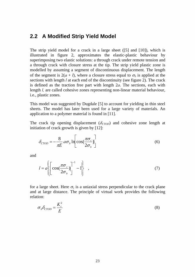
The strip yield model for a crack in a large sheet ([5] and [10]), which is illustrated in figure 2, approximates the elastic-plastic behaviour by superimposing two elastic solutions: a through crack under remote tension and a through crack with closure stress at the tip. The strip yield plastic zone is modelled by assuming a segment of discontinuous displacement. The length of the segment is 2(a + l), where a closure stress equal to σ is applied at the sections with length l at each end of the discontinuity (see figure 2). The crack is defined as the traction free part with length 2a. The sections, each with length l, are called cohesive zones representing non-linear material behaviour, i.e., plastic zones.

b

This model was suggested by Dugdale [5] to account for yielding in thin steel sheets. The model has later been used for a large variety of materials. An application to a polymer material is found in [11].

The crack tip opening displacement (δCTOD) and cohesive zone length at initiation of crack growth is given by [12]:

δCTOD = −8

πEaσ b ln cos(πσC

2σ b

)⎡

⎣ ⎢

⎤

⎦ ⎥ (6)

and

⎪⎭

⎪⎬⎫

⎪⎩

⎪⎨⎧

−⎥⎦

⎤⎢⎣

⎡=

−

1)2

cos(1

b

Calσ

πσ , (7)

for a large sheet. Here σc is a uniaxial stress perpendicular to the crack plane and at large distance. The principle of virtual work provides the following relation:

σ bδCTOD =Kc

2

E (8)

23

σb

a l

Figure 2. The strip yield model (l is the length of cohesive zone).

From equations (6) and (8), a relation between crack length a and applied stress σc at fracture can be derived as below:

⎥⎥⎦

⎤

⎢⎢⎣

⎡⎟⎟⎠

⎞⎜⎜⎝

⎛−= 2

2

8exparccos2

b

c

b

c

aKσ

ππσ

σ . (9)

Equations (6), (7) and (9) are limited to infinite plates. To make the results asymptotically reasonable for a finite plate when a → W the correction factor φ from (2) is used to modify (9) in the following way:

⎥⎦

⎤⎢⎣

⎡⎟⎟⎠

⎞⎜⎜⎝

⎛−= 22

2

8exparccos2

b

c

b

c

aK

σφπ

πσσ

. (10)

Here the geometry dependent φ is obtained through (3) or (4).

24

3 Experiments

3.1 Test of a Large Specimen with a Centred Pre- Crack

Tensile tests of large specimens with a pre-crack were performed on an MTS Universal testing machine with a modified grip. A centred crack panel (see figure 1a) was used. The specimen had a width 2W = 95 mm, height 2h = 230 mm and thickness t = 6.42 µm and, in the centre of the specimen, a pre-fabricated crack. All together 50 specimens were tested that included 10 different pre-crack lengths ranging from 2ao = 5 mm to 50 mm were used and for each crack length 5 specimens were tested. All tests took place in room temperature.

The modified grip of the tensile test machine is a pair of wide clamps shown in figure 3. The upper clamp was attached to a crosshead in the MTS-machine via a 2 kN load cell. Since the specimen was mounted vertically, the clamps were equipped with needles to facilitate a correct positioning.

420mm

Quick-acting lock nuts

Upper clamp Load cell

Uppercrosshead

Lowerclamp

Traversingcrosshead

Designed grip

Figure 3. Tensile test machine.

25

After the positioning of a sample, the upper and lower clamps were closed and a pressure was applied by tightening four equally spaced quick-acting locking nuts along the front of each clamp, see figure 3. Locking pins at the centre of the front jaws keep the clamps in an open position during mounting. The largest sample that can be accommodated is 420 mm wide.

Specimens were tested by traversing the upper crosshead and by placing the sample under increasing tension at a constant crosshead speed of 9.2 mm/min. The software TestWorks was used to control the load frame and also to record data. During testing the values of displacement and load were monitored and recorded. All tests were run until the entire cross section had fractured. Further details of the method have been given in [13].

3.2 In situ Test of a Single Edge Notched Specimen in a SEM

To study the fracture behaviour of very short cracks, a JEOL/JSM-5310LV Scanning Electron Microscope (SEM) with a tensile stage was used. A single edge notched tension (SENT) panel (see figure 1b) was placed 30 mm under the microscope sensor. The dimensions of the specimen were length L = 8 mm, height h = 4.5 mm and thickness t = 6.42 µm. A V-notch with the depth ao = 1 mm and 90o between edges were cut carefully by using a razor knife as shown in figure 1b.

The specimen was loaded using the tensile stage with a velocity of 0.08 mm/min. The deformation was observed during increasing straining of the specimen. Photographs from the microscope camera show the growing crack. The crack length was then measured on the photographs. The commercial program Adobe Photoshop was used to prepare the resulting images. The crack is assumed to be located only where the electron beam is not reflected, i.e. the crack is identified as the dark areas of the photographs.

To explore the fracture behaviour, further additional SENT specimens were tested outside the microscope. These specimens were provided with V-notches with ao = 0.8, 1.2, 1.6 mm made by using a water jet cutting machine and tested in the MTS tensile test machine.

The length, a, of the initiated and growing crack is measured from the free edge. The relation between critical stress and pre-crack length was studied. The detailed results can be found in [14].

26

3.3 Post-Test Fractographical Examination

A non-contact method using an optical microscope with a motorized stage was used to study the crack surface profile. A focus-detection based method was used. The technology is based on registering the local focal distance variations and scanning over the body surface. The local focus analysis is based on finding the maximum local image sharpness in the sense of maximum standard deviation of light intensity values for pixels surrounding a selected point. Separation of an image signal into three-colour channels minimise the chromatic aberration and improve the accuracy. The lateral position is given by a motorised table. The vertical resolution of the method is of the order of a few hundred nanometres. The table is calibrated and the resolution is around a micrometer. Further details on the method can be found in [15]. The accuracy is less than a micron.

4 Results and Discussion

4.1 Centred Crack Panel (CC)

Critical stresses for different crack lengths (5-50 mm) were measured. These results in the form of normalized critical stresses, σc /σb, versus normalized crack length, a, for the CC specimen is displayed in figure 4.

From this curve, σb can be found to be equal to 60 MPa , which is very close to the tensile test result in [16]. The least square method was used to select the resulting critical stress for each crack length for which five experiments were made. In figure 4, the analytical result using LEFM (5) and the result for the strip yield model (10) is included. Good agreement can be found between the measured results and the analytical results both with LEFM and SY models for crack lengths larger than 10 mm. For crack lengths less than 10 mm, the analytical results using the strip yield model show a close correlation with the measured values, whereas the LEFM mode fails to describe the experimental result for these short crack lengths.

27

0

0,5

1

1,5

2

0 0,2 0,4 0,6 0,8 1

a o /W

σ c/ σ

bLEFM, Eq.(9)SY model, Eq.(10)EXP.

Figure 4. Normalized critical stress versus normalized half of the initial crack lengths (Centred Crack panel, W=47.5 mm). The vertical axis shows the

normalized critical stress for a few crack lengths where 5 specimens were tested. The arithmetic average value was chosen.

The measured loads and computed stress intensity factors can be calculated using equation (2) and (3). However, one requirement for using (2) is that the non-linear region surrounding the crack tip is small compared to the crack length and remaining ligament to the traction-free edge ahead of the crack tip. This leaves us with a shortest and a longest possible crack length. Guided by the appearance of figure 4, the conclusion is that the lower limit could be around a = 10 mm. The upper limit for the crack length does not seem to be exceeded at the present experiments. Thus, the fracture toughness Kc = 6.1 MPam1/2 is obtained as the inserted straight line in figure 5. The line is inserted to make a reasonable correlation with the experimental results. This figure shows the normalized stress intensity factor for different crack lengths. For comparison the calculated results of the strip yield model (10) are also included in this figure. As mentioned earlier the strip yield model shows good agreement with the experimental results.

28

00,20,40,60,8

11,21,4

0 0,2 0,4 0,6 0,8 1

a o /W

σ cf(a

/w)( π

a)(1

/2) /

KC

EXP.ExtrapolatedSY-model,Eq.(10)

Figure 5. Normalized stress intensity factor versus normalized half of the initial crack length (Centred Crack panel, W=47.5 mm).

4.2 Single Edge Notched Panel (SENT)

The results for the CC panel indicate that there is a plastic zone with a substantial effect on fracture for crack lengths below 5 mm. This suggests that the linear extent of the plastic zone is at least a few millimetres. To study the fracture behaviour a growing crack was therefore followed in a SEM during monotonically increasing tension. For practical reasons the small SENT panel was chosen. Here, W = 4.5 mm, ao = 1 mm and the length of the specimen h = 8 mm. Photographs were taken during the growth and records of the load and the crack lengths were taken (see figure 6a and b). The crack grew in length from 1 to 2.43 mm.

The crack first follows a zigzag path. This behaviour decreases after some growth and the crack seems to grow more straight in a direction perpendicular to the edge of the specimen. The distance between the crack surfaces at applied load, as can be seen on the photographs, remains rather constant. Possibly, small cracks or voids are also present ahead of the crack tip (see (V) in figure 6b). The observation is uncertain and may be due to shadowing of the crack by the buckling foil.

29

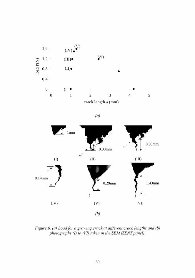
(a)

00 1 2 3 4 5

crack length a (mm)

0,4

0,8

1,2

1,6

load

P(N

)

(V) (IV)

(VI)(III)

(II)

(I)

(a)

(b)

Figure 6. (a) Load for a growing crack at different crack lengths and (b) photographs (I) to (VI) taken in the SEM (SENT panel).

(II)

0.03mm

1mm

(I)

0.08mm

(III)

0.14mm 1.43mm 0.29mm

(IV) (V) (VI)

30

The stress during the growth of the crack in figure 6 was recorded. The resulting crack is stable throughout the test because of the displacement control and the smallness of the specimen. However, even for a controlled load, the crack growth would be stable before the maximum load is reached. The maximum load occurs after around 0.3 mm of crack growth. This is somewhat surprising since this behaviour (i.e. stable crack growth at load control) requires plastic dissipation that increases during crack growth. This observation cannot be explained by the strip yield model. One possibility is that the plastic deformation spread in a region above and below the crack plane. This was, however, not observed in the present study.

00,20,40,60,8

11,21,41,61,8

2

0 0,2 0,4 0,6 0,8 1

a o /W

σ c/ σ

b

LEFM, Eq.(9)SY-model, Eq.(10)EXP1EXP2

Figure 7. Normalized critical stress versus normalized initial crack lengths (SENT panel), EXP1.: experiment result from a V-notched made by a sharp

knife. EXP2.: experiment result from a notch made by the water jet.

31

For the SENT panel and small crack sizes the critical stresses for notch lengths (ao = 0.8-1.6 mm) were also measured. The normalised critical stresses (σc/σb) versus normalised crack length (a/W) are given in figure 7 for the SENT panel. In the same figure, the analytical result found by using LEFM (5) and by using the modified strip yield model (10) is included. Good agreement can be found between the measured results and the analytical results with the modified strip yield model.

4.3 Necking - The Fracture Process

The experimentally determined fracture toughness was observed to decrease with decreasing foil thickness [4]. This is confirmed by the present study whereas the measured fracture toughness is 6.1 MPam1/2 as compared with the larger values of 20 to 50 MPam1/2 given in [17, 18]. Further, the crack tip opening displacement, measured to around 7 µm, suggests that fracture occurs through necking. Examination of the edge of the fractured foil, using the optical profilometric method described in section 3.3, provides visual evidence to this conclusion. The profile is shown in figures 8a and b. The slope has a depth of 3.2 µm as an average of the depth measured from both sides of the aluminium foil. This is very close to half of the thickness of the foil, which is 3.21 µm. The profile of a cut through the foil perpendicular to both the foil surface and the crack surface are shown in figure 9c. A slip-line theory provides a theoretical estimate of the slope for necking of any elastic plastic sheet. Figures 9a and b show the plastic deformation of the cross-section of a sheet. The equilivolumetric deformation requires a slope of 1:2 of the plastically deformed surface. The process continues until the thickness vanishes. Comparing the theoretical results (full lines) with the photographed cross-section (figure 9c) supports the belief that necking precedes the fracture. A slight thinning of the sheet, increasing towards the necking region, is observed. This may be due to some plastic deformation outside the necking region. It is known [19] that the cohesive zone model is incompatible with the associated flow rule for a von Mises material. Some plasticity outside the cohesive zone or necking region becomes necessary. A possibility is that the slight thinning of the cross-section near the necking region is a trace of that.

The necking type of the fracture process gives rise to the question of how the thin sheet behaves in a laminate. There is a possibility that the plastic deformation is constrained by the surrounding material. While fracture of the foil is of interest because of its contribution to laminates, the possible

32

interaction between the fracture processes in the different layers is important. In [29], it has been observed that there is very strong coupling between the individual layers of laminates at fracture. If that is due to a redistribution of the load in the crack tip region or due to a direct influence on the fracture processes is yet unknown.

Region with plastic yielding Foil surface

One of twocrack surfaces

Figure 8. Profile of the edge of the fractured foil, using the optical profilometric method [14].

33

Thic

knes

s

Cross section boundaries

(a)

Incr

ease

d di

spla

cem

ent

2 1

(b)

-6

-4

-2

0

2

4

6

-20 -18 -16 -14 -12 -10 -8 -6 -4 -2 0

distance from crack surface (µm)

thic

knes

s ( µ

m)

(c)

Figure 9. (a). Slip-line solutions for necking under uniaxial stress. ( b). The necking process occurs immediately before the final separation of the sheet.

(c). The image is obtained looking from the side to the neck of the crack.

34

5 Conclusions

From the results above, the following conclusions are drawn:

- The fracture toughness of the thin foil is much lower than the fracture toughness value of the aluminium given in handbooks.

- No fracture surface can be observed using optical profilometry under the microscope. Fracture seems to occur through so-called necking, i.e. the thickness in a line-shaped region ahead of the crack tip reduced to almost zero before crack propagation occurs. The plastically deformed cross-section resembles the one obtained for a slip-line theory for failure through simple plastic yielding. However, there is a vague indication of plasticity outside the necking region.

- A modified strip yield model is shown to provide a suitable model. This model leads to the conclusion that the crack tip is preceded by a substantial plastic zone as compared with the crack length.

Acknowledgements

This work was granted by Tetra Pak R&D AB, Tetra Brik Carton Ambient AB, Blekinge Institute of Technology and the Swedish Foundation for Knowledge and Competence Development. The authors are grateful to the Swedish National Testing and Research Institute (SP) for the SEM measurement, SCA Research AB for performing the tensile test of large specimen with pre-crack and to Mr. Bratov for measuring the crack surface. The authors would also like to thank WaterJet AB for preparing part of the specimens. Thanks also to Tech. Lic. Astrid Magnusson for valuable discussions.

35

References

1. Tryding, J., In-plane fracture of paper. Ph.D-thesis, Report TVSM-1008, ISSN: 0281-6679, Lund Institute of Technology, Lund, Sweden, 1996.

2. Xia, Q. S., Boyce, M. C. and Parks, D. M., A constitutive model for the

anisotropic elastic-plastic deformation of paper and paperboard. Int. J. of Solids and Structures, 2002, 39(15), 4053-4071.

3. David, J.R., Aluminum and Aluminum alloys. David & Associates, ASM

International, ISBN: 0-87170-496-X, 1994. 4. Maucher, H., Festigkeit und dehnung wreichgluhter aluminiumfolien

verschiedener reinheit und dicke. J. Aluminium, 1942, 316-319. 5. Dugdale, D.S., Yielding in steel sheets containing slits, J. of the Mech.

and Physics of Solids, 1960, 8, 100-104. 6. Ståhle, P., On the small crack fracture mechanics. Int. J. of fracture, 1983,

22, 203-216. 7. Williams, M.L., On the stress distribution at the base of a stationary crack.

J. of Appl. Mech. 1957, 24, 109-114. 8. Isida, M., Effect of width and length on stress intensity factors of

internally cracked plates under various boundary conditions. Int. J. Fract. Mech., 1971, 7, 301-316.

9. Tada, H., Paris, P.C., Irwin, G.R., The Stress Analysis of Crack

Handbook. Del. Research Corp., Lehigh, Bethlehem, PA, USA, 1973. 10. Barenblatt, G.I., The mathematical theory of equilibrium cracks in brittle

fracture. Adv. in Appl. Mech., 1962, 7, 55-129. 11. Anderson, T.L., Fracture Mechanics: Fundamentals and Applications.

Boca Raton, FL, USA, ISBN: 0-8493-4260-0, 1995. 12. Burdekin, F.M. and Stone, D.E.W., The crack opening displacement

approach to fracture mechanics in yielding materials. J. of Strain Analysis, 1966, 1, 145-153.

36

13. Hägglund, R., Fracture mechanical modelling of embossed paper.

Licentiate thesis, Report 2001:26, ISSN: 1402-1757, Dept. of Mech. Eng., Luleå Univ. of Tech., Sweden, 2001.

14. Kao-Walter, S., Mechanical and fracture properties of thin Al-foil.

Research report, Blekinge Inst. of Tech., 2001:09, Karlskrona, Sweden, 2001.

15. Bratov, V., A method to study surface profiles using automated optical

microscope. MUMAT 2002:11, report from Div. of Material Science, Malmö, Sweden, 2002.

16. Kao-Walter, S., Dalström, J., Karlsson, T. and Magnusson, A., A study of

the relation between the mechanical properties and the adhesion level in a laminated packaging material. Mech. of Comp. Mat., 2004, 40(1), 29-36.

17. Sundström, B., Handbok och Formelsamling i Hållfasthetslära. Fingraf

AB, Södertälje, Sweden, 1998. 18. Pardoen, T., Marchal, Y. and Delannay, F., Essential work of fracture

compared to fracture mechanics - towards a thickness independent plane stress toughness. Eng. Frac. Mech. 2002, 69, 617-631.

19. Rice, J.R., Mathematical analyses in the mechanics of fracture. Fracture:

an Advanced Treatise II, H. Liebowitz ed., Academic Press, 1968, New York, USA, 191-308.

20. Kao-Walter, S., Ståhle, P. and Hägglund, R., Fracture toughness of a

laminated composite. Fracture of Polymers, Composites and Adhesives II, Elsevier Science, Blackman, B. R. K. Pavan, A. and Williams, J. G. (Eds.), ISBN: 0-08-044195-5, 2003,Oxford, UK, 357-364.

37

38

Paper B

A Study of the Relation between the Mechanical Properties and

the Adhesion Level in a Laminated Packaging Material

39

Paper B is published as:

Kao-Walter, S., Dalström, J., Karlsson, T. and Magnusson, A., A study of the relation between the mechanical properties and the adhesion level in a laminated packaging material. Mech. of Comp. Mat., 2004, 40(1), 29-36.

40

A Study of the Relation between the Mechanical Properties and

the Adhesion Level in a Laminated Packaging Material

Kao-Walter, S., Dalström, J., Karlsson, T. and Magnusson, A.

Abstract

Mechanical properties of a laminate were studied in relation to the adhesion level. A special application for the liquid food packaging material is considered. The material is laminated by aluminium-foil/adhesive/polymer. A theory of mechanics for composite materials was used to evaluate experiments. In the experiments, laminates with the adhesive layer and without the adhesive layer were tested. Tensile tests were first made for every layer of the laminate and the results were then used to analyse the results from tensile tests of the entire laminate as well as in calculations. Relations between different mechanical properties such as Young’s modulus, peak stress as well as strain at peak stress and the adhesion level were analysed. It was found that the tensile strength and the strain at peak stress increased when the adhesion level increased. Only a slight difference of Young’s modulus was observed at different adhesion levels.

41

1 Introduction

Liquid food packages are often made from packaging material, which consists of several different layers of material for the different requirements of the package. It is very important to secure that every layer keeps its function during the filling and transportation process. A special application for the liquid food packaging material is considered. The laminate consists of carton, LDPE (Low Density Polyethylene), Al-foil (aluminium foil) and an adhesive layer. Several works have been done to study the different mechanical properties of these materials [1-5]. The purpose and aim of the work was to study the mechanical properties of a laminate in relation to the adhesion level. The theory of mechanics of composite materials, experiments and the finite element method were used. In the experimental part of the work, laminates with different adhesion levels were prepared. Tensile tests were made for every layer, as well as for the entire laminates. The experimental results were then compared with the results calculated by applying the analytical equations and the finite element method. The measured properties for the individual layers were used for theoretical calculations according to the laminate theory. The analysis of mechanical properties of laminated materials is based on the assumption that there is perfect adhesion between the layers. This is not always the case for packaging materials. It is therefore interesting to find how the mechanical properties of the laminate are influenced by the adhesion level between the layers. It is essential to be aware of the fact that the laminate theory applied here is only valid in the elastic region. A finite element model based on the experimental results was also done to simulate the entire stress-strain diagram. The simulations were made both on the elastic and the plastic region. One advantage with the finite element model is that the stress is obtained in each layer, compared to the experiment where only the stress-strain relation for the entire laminate is obtained.

42

2 Materials

A laminate is a stack of lamina, oriented in a specific manner to achieve a desired result [6]. It could be of the same material or a combination of several different materials. The mechanical response of a laminate is different from that of the individual lamina. The response of the laminate depends on the properties of each lamina and the order in which the lamina are stacked. The laminate in this work consists of Al-foil/Adhesive/LDPE. LDPE is in reality not linear, but at small strains it can be approximated with a linear elastic material [7]. It can also be considered to be isotropic. The adhesive layer is assumed to have the same mechanical properties as LDPE. An adhesive has to counteract the effects of surface roughness [8]. It has to fill the valleys and to remove surface impurities. If it does this, a continuous contact between the solids (often called adherends) and the adhesive is established, and the new three-layer solid (consisting of adherend-adhesive-adherend) has a notable strength. In this work the influence of the adhesion level is investigated. Adhesion appears between surfaces, either naturally when LDPE is moulded on the adherend or with an adhesive layer. If there is not perfect adhesion, delamination will occur, i.e. some parts between the two surfaces will not be connected. When delamination appears, the laminate may have other properties than a laminate with perfect adhesion. For packages, the function of the aluminium foil is to prevent oxygen from reacting with the contents of the package and also to act as a barrier against light. The function of the LDPE layer is to act as a moisture barrier as well as to protect the liquid from reacting with the aluminium foil. The paperboard gives the stiffness and the strength of the package. The order of the different layers is shown in figure 1.

43

LDPE

AdhesiveAluminium

LDPE

Paperboard

LDPE

Figure 1. The laminate package material.

There are three types of main materials: aluminium foil, LDPE and paperboard (not discussed in this paper). The materials studied in this work are chosen as below:

• C1: Al-foil (6.25 µm)

• C2: LDPE (27.30 µm)

• C3: LDPE (27.30 µm)/1Adhesive(7,10 µm) /Al-foil (6.25µm)

• C4: LDPE (27.30 µm)/Al-foil (6.25µm)

• C5: LDPE (27.30 µm)|| 2Al-foil (6.25µm).

1 / Adhesion between the layers during the manufacturing process (glued). 2 || No adhesion between the layers (not glued).

44

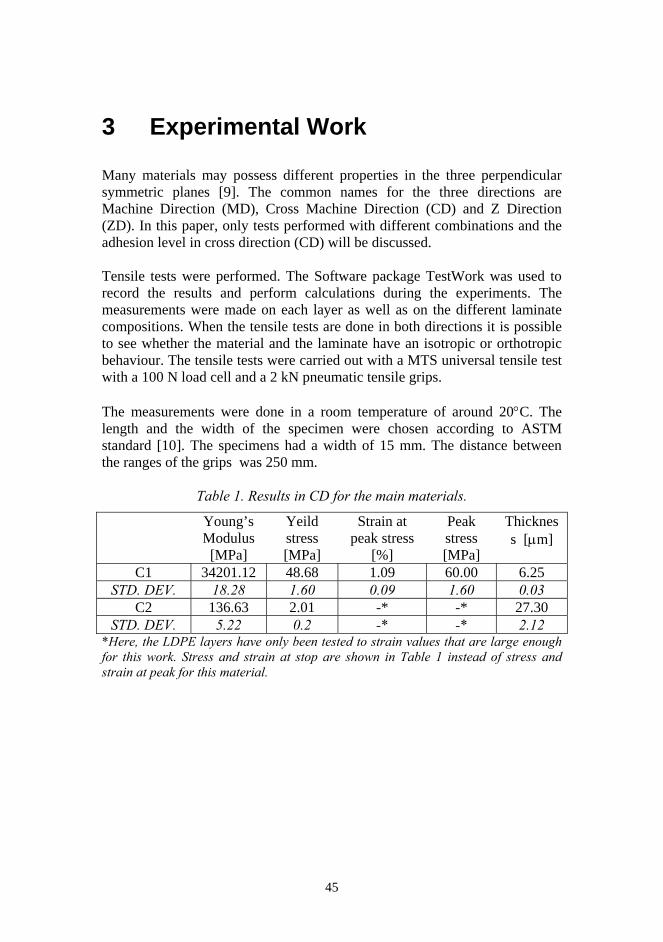
3 Experimental Work

Many materials may possess different properties in the three perpendicular symmetric planes [9]. The common names for the three directions are Machine Direction (MD), Cross Machine Direction (CD) and Z Direction (ZD). In this paper, only tests performed with different combinations and the adhesion level in cross direction (CD) will be discussed. Tensile tests were performed. The Software package TestWork was used to record the results and perform calculations during the experiments. The measurements were made on each layer as well as on the different laminate compositions. When the tensile tests are done in both directions it is possible to see whether the material and the laminate have an isotropic or orthotropic behaviour. The tensile tests were carried out with a MTS universal tensile test with a 100 N load cell and a 2 kN pneumatic tensile grips. The measurements were done in a room temperature of around 20°C. The length and the width of the specimen were chosen according to ASTM standard [10]. The specimens had a width of 15 mm. The distance between the ranges of the grips was 250 mm.

Table 1. Results in CD for the main materials.

Young’s Modulus

[MPa]

Yeild stress [MPa]

Strain at peak stress

[%]

Peak stress [MPa]

Thickness [µm]

C1 34201.12 48.68 1.09 60.00 6.25 STD. DEV. 18.28 1.60 0.09 1.60 0.03

C2 136.63 2.01 -* -* 27.30 STD. DEV. 5.22 0.2 -* -* 2.12

*Here, the LDPE layers have only been tested to strain values that are large enough for this work. Stress and strain at stop are shown in Table 1 instead of stress and strain at peak for this material.

45

Table 2. Results in CD for the different laminate compositions.

Young’s Modulus

[MPa]

Strain at peak stress [%]

Peak stress [MPa]

Thickness [µm]

C3 4609.36 4.56 15.70 40.65 STD. DEV. 9.79 1.10 0.50 1.20

C4 4645.44 2.27 15.19 33.55 STD. DEV. 19.28 0.62 0.92 0.87

C5 4588.50 1.28 12.50 33.55 STD. DEV. 8.36 0.76 0.78 1.16

Mechanical properties for the main material C1 and C2 were measured. The average values of the results were used in further calculations and are presented in Table 1. The thickness of each specimen was measured at several places and an average of the thickness was used as a setting for the software. For all tests a constant strain rate of 4 %/min was chosen. Mechanical properties for the laminate C3, C4 and C5 were measured. It is essentially to recognise that the tests are just performed until there is a rupture in the Al-foil. These results are presented in Table 2. Some of the results and the details about the methods can be found in a separate report [11].

4 Theoretical Work

It is possible to determine a Young’s modulus for the complete laminate when the Young’s modulus and the thickness are known for each layer [12], [13]. Hooke’s law for linear elastic material in the state of plane stress can be written as

46

[ ]

[

⎪⎪⎪

⎩

⎪⎪⎪

⎨

⎧

=

+−

=

+−

=

xyxy

xyy

yxx

G

E

E

γτ

νεεν

σ

νεεν

σ

2

2

1

1

] . (1)

In assuming that all the layers in the laminate are perfectly laminated, the strain in the different layers will be equal to the strain for the entire laminate

iεε = . (2) ,...2,1=i

This is only valid until some of the materials expose a rupture. By equilibrium equations, the total force on the laminate must be equal to the sum of the forces in each of the individual layers

∑= iL FF . (3)

Now the average stress in the laminate can be determined since the stress is equal to the force divided by the area. In this case the total force is the sum of the forces in each layer and the total area is the sum of the areas in each individual layer. The average stress then becomes

∑∑=

i

iL A

Fσ . (4)

Each layer in the laminate has the same width, which therefore can be eliminated. Equation (4) can then be rewritten as

∑∑=

i

iiL t

tσσ . (5)

By inserting equation (1), (2) into (5), the Young’s modulus of the laminate is obtained

47

( ) ⎟⎟⎠

⎞⎜⎜⎝

⎛

−

⎟⎟⎠

⎞⎜⎜⎝

⎛

−−⎟

⎟⎠

⎞⎜⎜⎝

⎛

−=

∑∑

∑∑

2

2

2

2

2

1

11

i

iii

i

iii

i

ii

LtE

t

tEtE

E

ν

νν

ν . (6)

This formula is known as the laminate theory and makes it now possible to calculate the Young’s modulus of the laminate in a theoretical manner. If the layers in the laminate have the same value of Poisson's ratio, the equation (6) will be become

∑∑=

i

iiL t

tEE . (7)

By implementing equation (6) and (7) in MatLab[14] and using the experimentally established results for the main materials, Young’s modulus could be obtained for the laminated packaging material. Here, the small strain values that are less than 0.35% are used in the calculation. In the plastic region, the strain can be divided into two parts [15]

plel εεε += . (8)

Here, εel is the elastic strain and can be calculated by Eq.(1). εpl is the plastic strain. In the finite element calculation, an isotropic, linear hardening plastic model was used for each layer[16]. Thus, the theoretical results can even be obtained in the plastic region.

5 Finite Element Calculation

A model of the specimen was also simulated in ABAQUS 6.2 [16]. A four-node thin shell element, S4R5 was chosen for the model. Since the geometry and the expected deformations are symmetric, only a quarter of the specimen needs to be used in the model. The model of the specimen was 7.5 mm in x- and 125 mm in y-direction. The resulting model in the analysis had a mesh

48

consisting of 5 elements in x- and 79 elements in y-direction. All the elements had the same size. An elastic-plastic von Mises model with isotropic hardening was used for each layer with the material parameters taken from the experiment results as shown in Tab.1 and Tab.2. The calculations have been performed until a 4% strain is obtained. The aluminium foil is the most brittle material in the laminates and rupture happens at approximately 1% strain. The simulated calculations do not consider delamination or rupture and are therefore only valid until the foil begins to delaminate from the other layers in the laminate. It is difficult to predict when the delamination starts, but certainly before 4%.

6 Results and Discussion

The mechanical properties of a package have a great influence on the behaviour and the functionality during its lifetime. Based on the results from the theoretical calculation and the experiment work, the influence of the adhesion level on the mechanical properties of the Al-foil and LDPE can be found. In the following, several comparisons will be done for the laminate. 6.1 The Influence of Adhesion on Young’s

Modulus

Figure 2 shows the result of Young’s modulus of the Al-foil and LDPE laminate with different adhesion levels. Perfect adhesion is the case where the Young’s modulus of the Al-foil and LDPE has been calculated by the theoretical equation (7). To find the influence of Poisson's ratio to the Young's modulus, calculations has also been done by inserting different values of Poisson's ratio for Al-foil and LDPE/Adhesive. Equation (6) has been used here and Poisson's ratio are chosen as νAl=0.3 [4] and νLDPE=0.4 (assumed). Results for the cases (C) and (D) are taken from the experimental results.

49

0

2000

4000

6000

8000

(A ). (B ). (C ). (D ). (E ). (F )

You

ng's

Mod

ulus

[MPa

]

M in im um V alueA verage V alueM axim um V alue

Figure 2. Young’s modulus in relationship to the adhesion level. (A). Eq.(7), with adhesive layer. (B). Eq.(6), with adhesive layer. (C). Experimental

results, Case 3. (D). Experimental results, Case 4. (E). Experimental results, Case 3. (F). Eq.(6), without adhesive layer.

6.2 The Influence of Adhesion to Strain at Peak

Stress

Figure 3 shows the result of the strain at peak stress of the Al-foil and LDPE laminate with different adhesion levels. It was observed that rupture of Al-foil happened at peak stress for all the laminate cases. Results for the cases of C3, C4 and C5 are taken from the experimental average curve. The results show that strain values at peak stress will be much higher with increasing adhesion level.

50

0

1

2

3

4

5

6

C3 C4 C5 C1

Stra

in a

t Pea

k St

ress

[%]

Minimum ValueAverage ValueMaximum Value

Figure 3. Strain at peak stress depends on the adhesion level.

6.3 The Influence of Adhesion to Peak Stress

By Table 2, it can be concluded that the higher adhesion level will lead to higher peak stress in the laminate. It was observed that during the experiment rupture of Al-foil happened around the peak stress in the laminate. Figure 4 shows the result of stress at rupture in Al-foil at different cases. Equation (3-5) is used to calculate the stress at rupture of the Al-foil based on the experiment results. Since there is force equilibrium between the layers, It is possible that the sum of the forces in each layer is equal to the total force in the laminate. Here, the strain is the same for all layers. In the calculation, the stress in LDPE layer is taken at the strain where the aluminium foil ruptures. All three laminate cases are calculated. Again, stress at rupture in Al-foil increases when increasing the adhesive level.

51

0

10

20

30

40

50

60

70

80

90

100

From C3 From C4 From C5 From C1

Stre

ss a

t rup

ture

in A

l-foi

l [M

Pa]

Figure 4. Stress at rupture in Al-foil depends on the adhesion level.

6.4 Experiment Compared with Simulation

In figure 5, the load-displacement results obtained by experimental and simulation for the LDPE/Adhesive/Al-foil laminate have been compared. In addition, the experiment results for each layer are shown in the same figure. Comparison between the experimental and simulated results showed a good agreement until the rupture occured in the experiment. The simulation has been done with two different boundary conditions where the force/displacement is applied as it was described above. The results are almost the same.

52

0

10

20

30

40

50

60

70

0 1 2 3 4 5

Strain [%]

Stre

ss [M

Pa]

ExperimentalSimulatedAl-foilLDPE

Figure 5. Comparison in cross machine direction.

7 Conclusion and Further Work

The mechanical properties of LDPE/Adhesive/Al-foil, LDPE/Al-foil and LDPE||Al-foil have been investigated. Perfect adhesion is only obtained with the theoretical calculation. Both the peak stress (or tensile strength) and strain at rupture increased when the adhesion level increased. During the experiment, delamination in the laminate can be found for cases 3 and 4. It was also observed in some of the specimens that several small cracks appeared before the loading stress reached the ultimate value for the laminate with adhesive layer. Further work will be done by analysing fracture behaviour by applying the theory of fracture mechanics in laminate. However, very small differences of Young’s modulus were found by increasing the adhesion level. It should be pointed out that the aim of this work was to find the influence of the adhesion level on the mechanical

53

properties of laminate. More works need to be done in order to obtain the Young’s modulus as well as Poisson’s ratio of the materials accurately.

Acknowledgements

This work was granted by Tetra Pak Carton Ambient AB. The Authors would like to thank Prof. Per Ståhle and Dr. Claes Jogréus for valuable discussions. Thanks also to Mr. K. Asplund and Mr. E.M. Mfoumou for preparing the experimental material.

References

1. Jones, R. M., Mechanics of composite materials. Second Edition. Taylor and Frances, Inc., 1999.

2. Warren, R., Composite Materials. Inst. för Metalliska

Konstruktionsmaterial, CTH, 1986/87. 3. Kao-Walter, S. and Ståhle, P., In situ SEM study of fracture of an ultra

thin Al-foil - modelling of the fracture process. SPIE 3rd ICEM proceeding, ISBN: 0-8194-4261-5, Wu, X., Qin, Y., Fang, J., Ke, J. (eds.), Beijing, China, 2001, 253-256.

4. Tryding, J., In-plane fracture of paper. Ph.D-thesis, Report TVSM-1008,

ISSN: 0281-6679, Lund Institute of Technology, Lund, Sweden, 1996. 5. Stenberg, N., Fellers, C., Östlund, S., Measuring the stress-strain

properties of paperboard in the thickness direction. JPPS, 2001, 27 (6). 6. Tsai, Stephen W., Hahn, H. Thomas, Introduction to composite materials.

ISBN: 0-87762-288-4, Technomic Publishing Company Inc., Pennsylvania, U.S.A., 1980.

7. Beldie, L., Svensson, C., Accurate stress distribution in laminated

package materials. Master’s Thesis, Solid Mechanics Lund Institute of Technology, Lund, 1998.

54

8. Bikerman, J.J., The Science of Adhesive Joints. Second edition, Academic Press Inc., 1968.

9. Persson, K., Material model for paper experimental and theoretical

aspects. Diploma Report, Solid Mechanics Lund Institute of Technology, 1991.

10. ASTM D-882-91, Standard test methods for tensile properties of thin

plastic sheeting. American Society for Testing and Materials, Philadelphia, Pa., 1991.

11. Dahlström, J., Karlsson, T.- Mechanical analysis of laminated packaging

material. Master’s Thesis, Department of Mechanical Engineering Blekinge Institute of Technology, Karlskrona, 2002.

12. Staab, George H., Laminar Composites. Butterworth- Heinemann, 1999. 13. Tan, Seng C. Stress Concentrations in Laminated Composites. ISBN: 1-

56676-077-1, Technomic Publishing Company Inc., Pennsylvania, U.S.A., 1994.

14. The Math Works Inc., MATLAB: The Language of Technical Computing.

Natick, MA USA: The Math Works Inc., 2000. 15. Hill, R., The Mathematical Theory of Plasticity. Oxford University Press

Inc., 1950. 16. ABAQUS, User’s Manual, Version 6.2, Hibbitt, Karlsson & Sorensen,

Inc., USA, 2001.

55

56

Paper C

Fracture Toughness of a Laminated Composite

57

Paper C is published as:

Kao-Walter, S., Ståhle, P. and Hägglund, R., Fracture Toughness of a Laminated Composite. Fracture of Polymers, Composites and Adhesives II, Elsevier Science, Blackman, B. R. K. Pavan, A. and Williams, J. G. (Eds.), ISBN: 0-08-044195-5, 2003, Oxford, UK, 357-364.

58

Fracture Toughness of a Laminated Composite

Kao-Walter, S., Ståhle, P. and Hägglund, R.

Abstract

The fracture toughness of a polymer-metal laminate composite is obtained by mechanical testing of a specimen containing a pre-crack. The laminate is a material used for packaging. It consists of a thin aluminium foil and a polymer coating. A centre cracked panel test geometry is used. Each of the layers forming the laminate is also tested separately. The result is compared with the measured fracture strength of the individual layers. It is observed that the load carrying capacity increases dramatically for the laminate. At the strain when peak load is reached for the laminate only aluminium is expected to carry any substantial load because of the low stiffness of the LDPE. However, the strength of the laminate is almost twice the strength of the aluminium foil. The reason seems to be that the aluminium forces the polymer to absorb large quantities of energy at small nominal strain. The toughness compares well with the accumulated toughness of all involved layers. Possible fracture of the interface between the layers is discussed.

59

1 Introduction

Liquid food packages are often made of packaging materials consisting of different material layers to fulfill several requirements of the package. It is very important to ensure that every layer maintains its function during the forming, filling and transportation processes. As an example here, a liquid food packaging material is considered. This is a laminate consisting of LDPE (Low Density Polyethylene) and an aluminium foil (Al-foil). Several studies of different mechanical properties of these materials have been performed [1-5]. It was found in [2] that aluminium foil and LDPE laminated together provide significantly higher stress and strain at fracture as compared with the simplified analytical prediction. Related works can also be found in [6], [7], [8] where notched tensile strength, fracture toughness as well as fatigue resistance for fiber/aluminium composite laminate were studied. The purpose of this work is to study the fracture toughness of a laminated material in relation to the adhesion between the layers. Load and extension were measured for a two-layer laminate specimen with a pre-crack as well as for the individual layers of the laminate. The same specimen geometry was used in all tests. For comparison, measurements were also done for the laminate without any adhesion between the layers.

2 Material

Laminate in this work consists of Al-foil and Low Density Polyethylene (LDPE). Fully annealed AA1200 Al-foil and LDPE with the product name LD270 is used.

Load versus extension were measured for the following materials:

Case 1: Al-foil with the thickness 8.98 µm.

Case 2: LDPE with the thickness 27.30 µm.

Case 3: Al-foil / LDPE – Al-foil coated by LDPE and the total thickness is 36.28 µm.

60

Case 4: Al-foil // LDPE – Al-foil and LDPE joined together without adhesion between the layers and the total thickness is 36.28 µm.

Here “/” applies to two material layers bonded together and “//” applies to two layers put together without any adhesion in between.

For case 3, pieces of Al-foil were cut from a roll of fabricated material as shown in figure 1(a). The laminate in case 3 was then prepared in a Haake film extruder with a 36 µm Polyester (PET) as carrier (see figure 1(b)). The foil was mounted on the PET carrier while LDPE was extruded and coated on Al-foil at a melting temperature of 278 oC. A nip with the pressure 202 bar was used to press the layers together. The laminated specimen for case 3 was then cut from the roll including PET/Al-foil/LDPE as shown in figure 1(c). After producing the material for case 3, LDPE was continuously extruded on the PET carrier under the same conditions but without the Al-foil. By peeling off the PET carrier, the LDPE produced here was used for making the specimen for case 2 and case 4. And the specimen of case 1 is taken from the Al-foil roll of the same direction as the other cases.

Figure 1. Schematic description of specimen preparing.

61

3 Experimental Method

Centre cracked panels as shown in figure 2(a) are used for evaluating the fracture toughness of the laminated composite and components of it. Pre-fabricated cracks are manually cut, using a razor blade, to a total slit length of 2a = 45 mm. The width and gauge length of the specimens was 2W = 95 mm and 2h = 230 mm, respectively.

Figure 2. Specimen and experiment set up. (a). Centre cracked panel.

(b). Set-up for fracture mechanical testing of laminated composites. The specimen shown here is case 4.

62

A pair of wide clamps is utilised, see figure 2(b). The tests are made in a MTS Universal Testing Machine. The upper clamp is attached to a 2.5 kN load cell as well as a crosshead in the MTS-machine. Since the specimen is mounted vertically, the clamps are equipped with needles to facilitate a correct positioning. After the positioning of a sample the upper and lower clamps are closed and the pressure is applied by tightening four equally spaced quick-acting locking nuts along the front of each clamp, see figure 2(b). Locking pins at the centre of the front jaws keep the clamps in an open position during mounting. The largest sample that can be accommodated is 420 mm wide. Specimens are tested by traversing the upper crosshead up to move the sample under increasing tension at a constant crosshead speed of 9.2 mm/min. The software TestWorks is used to control the load frame and also to record data. During testing, both the displacements between the crossheads and the load are monitored and recorded. All tests are run until the entire cross-section has fractured.

4 Analytical Approach

4.1 Elastic Behaviour of the Specimen

The force elongating the specimen may be separated into that of the unbroken specimen, Po, and the reduction, Pc, due to the presence of a crack. The former is calculated as follows:

Po =

uEWth

, (1)

and the latter is obtained from the energy, Uc, released during the cutting of a crack [6]:

Uc =

tE

KI2

0a∫ d ′ a . (2)

The stress intensity factor for the crack is given by

KI =

uE

h(1−ν 2)φ(a /W ). (3)

63

This gives the energy

Uc =

12

uPc =u2EWt

4h(1−ν 2 )φ(τ )

0

a /W

∫ dτ . (4)

Using φ given in [9] the integral of (4) is found to be 0.08 for a/W = 0.47. With W = 47.5 mm and h = 115 mm (1), (3) and (4) we get

⎥⎦

⎤⎢⎣

⎡−

+=−= ∫Wa

co dh

uEWtPPP/

02 )()1(2

11 ττφν

(5)

and

P = 0.92 uEWt

h. (6)

Thus, the stiffness of specimen decreases only 8% as compared with a corresponding unbroken specimen.

4.2 Crack Driving Force G

According to the theory of fracture mechanics, a crack driving force G is defined as the rate of change in potential energy per crack area and per unit of length of crack front [10, 11]. It is assumed that the critical driving force, Gc, of a crack in a single layer is constant and independent of whether the layer is bonded to other layers or not. Assuming that no delaminating occurs during the growth of a crack in the laminate and that energy is not dissipated in the material, the crack tip driving force for the laminate is the accumulated driving force for all layers, i.e.

G =

G1t1 + G2t2t1 + t2

(7)

Here, the assumption that G = GC as the crack growth criterion is examined. This criterion is valid if the crack grows in an approximately steady state. The load at onset of crack growth is usually regarded to define the fracture toughness. For materials with considerable toughening the incipient growth of

64

the crack leads to increased fracture toughness. At small scale yielding the maximum toughness may be of interest but in the present analyses the yielding is considerable. There is a difficulty to define onset of crack growth. Since the observation shows the crack grows in the Al-foil until the crack traverses the entire specimen before there is any substantial crack growth in the LDPE layer. 4.3 Peak Load and Dissipated Energy

For practical use the maximum load carrying capacity may be limiting the reliability of the packaging structure. Therefore it is interesting to compare peak load both for each material separately and as a laminate. It is also interesting to examine the energy dissipated before breaking is reached. The dissipated energy, U, is found from the load displacement curve, P(δ) as follows

U = P(τ )dτ

0

δ∫ −

dPdδ dδ<0

δ2

2 (8)

The second term represents the recovered elastic energy stored in the specimen. At the point marked with triangles (see curves from case 3 and case 4 in figure 4) the crack has grown in the Al-foil and traversed the entire specimen whereas the crack in LDPE in most cases did not grow at all. The average strain at peak load is still in the elastic regime for the LDPE material. A first assumption would therefore be that the entire energy is due to the fracture of the aluminium and that the LDPE does not contribute to the fracture toughness. The motivation for the interest in only the dissipated part of the energy is that the elastic part may be recovered which means that accumulated energy, e.g. a shockwave may temporarily overcome the barrier that the elastic energy represents. If this results in crack advance the recovered energy is restored which may lead to rapid crack growth.

65

5 Results and Discussion

5.1 Calibration of Load Cell

A load cell of 2.5 kN has to be used because of the relatively large weight of the clamp. Prior to testing, the 2.5 kN load cell was calibrated and the accuracy was investigated. The result for the comparison with 100 N load cells is shown in figure 3. It can be seen that the deviation is around 0.03% for loads larger than 5 N and in the interval 1 N to 5 N the error is less than 0.08%. 5.2 Measurements

Measurements are made on a centre cracked panel as described above. The specimen is loaded via the clamps attached to the ends of the specimen.

The test speed is 9.2 mm/min that gives a constant strain rate of 4% per min according to ASTM standard [12]. For each curve, five specimens are tested in room temperature. The averaged curves for the four materials are displayed in figure 4. This figure shows the force versus the extension diagram for the single layers together with the laminate.

Dev. of measured value from 2.5 kN load cell

-0,06-0,04-0,02

00,02

0,040,060,080,1

0 10 20 30 40

Load (N)

devi

atio

n (%

)

Figure 3. Difference in % between measurements of a 100 N load cell and the 2.5 kN load cell that is used in the experiment.

66

For each case, the specimen was extended until the crack grew through the entire specimen and broke into two peaces. For case 3 (Al-foil coated by a LDPE layer), it can be found that the maximum load value is the highest of all four cases. It was observed that the crack grows only in the Al-foil layer until the curve comes to the point that is marked with a triangle where the crack in Al-foil traverses the entire specimen. Similar observations have been made for case 4 in the beginning of the curve. After passing the triangular point where the crack in Al-foil traverses the entire specimen, the curve follows the curve of case 2 very well since there is only a single layer of LDPE remaining. By experiment results maximum force Fm, dissipated energy before the onset of fracture Am, total dissipated energy Atot as well as estimated stiffness dF/de in the elastic region are calculated and shown in Table 1. From these values and the diagrams in figure 4 the results can be analyzed and discussed as follows. The stiffness dF/de may be used together with (6) to predict the modulus of elasticity. The estimated modulus of elasticity is 9.3 GPa for Al-foil and 92.9 MPa for LDPE. The modulus of elasticity for aluminum is much smaller than expected (34 GPa in [2]). On the other hand, the modulus of elasticity for LDPE is rather close to the value from the earlier measured result (136 MPa in [2]). The measured displacements in the elastic region are therefore very uncertain and the stiffness results cannot be regarded as reliable. However, for case 4, the peak load was found to be slightly larger than peak load for the Al-foil alone. The peak load 14.2 N may be compared with the peak load of aluminum 12.9 N. The elongation at peak load of aluminum is 0.84 mm and the estimated stiffness in the elastic regime of LDPE is 0.97 N/mm. The latter gives an expected peak load of 12.9 + 0.84 x 0.97 = 13.7 N which is within 5% of the measured result (14.2 N).

67

Figure 4. Load versus extension for centre cracked panels. The diagram in (a) shows the results for one of the 5 tests from case1 to case 4. The standard deviation of the peak load is shown on the curve for each case. The picture

above was taken when the load for case 3 reaches the peak load. The diagram in (b) shows the detail result at extension from zero to 5 mm.

68

Table 1. Calculated values. Fm is the maximum force, Am is the area under the curve from zero to maximum force. Atot is the total area under each curve of

figure 4. dF/de is the stiffness in the elastic region. Max and min refers to the largest and the smallest values obtained among the five tests.

Cases 1. Al-foil 2. LDPE 3. Al/LDPE 4. Al//LDPEFm [N] 12.9 10.0 22.5 14.2 Fm max 16.3 10.3 23.5 15.8 Fm min 10.2 9.8 20.2 12.0

Am [N mm] 6.3 114 32.7 8.1 Am max 7.7 118 37.6 8.9 Am min 5.7 111 26.7 6.3

Atot [N mm] 13.6 257 238 247 Atot max 15.5 264 331 273 Atot min 10.1 252 191 253

dF/de [N/mm] 31.1 0.97 25.3 25.6 dF/de max 39.4 1.0 42.4 45.4 dF/de min 23.2 0.9 15.0 14.1

For case 3, the laminate of LDPE and Al-foil joined together displays a much higher peak load and larger extension at peak load. The value of this peak load of 22.5 N was found to be very close to the summation of peak load of Al-foil (12.9 N) and peak load of LDPE (10 N). During the test, small scale delamination between the layers was observed. The area under the load deflection curve, i.e., the energy required, is observed to be very large (32.7 N mm) compared with the energy required to break the Al-foil (13.6 N mm) and stored in the LDPE at the corresponding strain (3.0 N mm). Direct visual inspection of figure 4 shows that an astonishingly much larger amount of energy is consumed in the laminated material at moderate tension. The reason for this could be that the extension of LDPE requires multiple fracture of the Al-foil or delaminating. Multiple fracture of the Al-foil would consume a large amount of energy. Examination of the total energy consumed during complete fracture of the specimens for case 1, 2, 3 and 4 reveal that almost the same total energy is consumed at complete fracture irrespectively of if the layers are bonded together or not. Here, energy required to break Al-foil is 13.6 N mm and 257 N mm for the LDPE layer.

69

This may be compared with the energy, 238 N mm, required to break the laminate (case 3) and 247 N mm, required to break both layers of material in case 4. It is believed that less energy is consumed during the fracture of the LDPE in the laminated case because the straining of the LDPE is concentrated to the thin gap that is defined by the broken Al-foil. The energy for onset of the fracture in the Al-foil (Am

Al = 6.3 N mm) is certainly consumed already when the laminate has reached its peak load (compare to Am

Al/LDPE = 32.7 N mm). However, unexpectedly also the energy to break the laminate is almost entirely consumed at small straining of the specimen. The reason for this has to be sought in the mechanics of the fracture process region.

The almost equal energies in case 4 and 3 rule out the hypothesis of presence of additional dissipative processes in the laminate as an explanation for the much higher toughness of the laminate. One observes also that more energy is consumed at small strains and, hence, less at larger strains. Further, the peak load for the laminate is almost the same as the sum of the peak load for the Al-foil and the peak load for the LDPE layer. This suggests that the fracture processes distribute strain so that peak load occurs simultaneously in both materials. This is anticipated for a laminate with little delamination. The assumption is that both materials reach peak stress in a small process region in the vicinity of the crack tip.

6 Conclusions

An experimental investigation was performed on a laminate and separately on the individual components of the laminate. Peak load, energy dissipation at onset of fracture and at fast fracture were investigated. The fracture toughness cannot easily be defined because of very large scale yielding. Therefore, an alternative toughness measurement was proposed.

The following observations were made:

- Onset of crack growth was observed to occur approximately at peak load. In the laminate, fracture of LDPE occurred after completed failure of the Al-foil.

-Peak load for the laminate is almost the same as the sum of the peak load for the Al-foil and the peak load for the LDPE layer. This suggests that both materials reach peak stress in a small region in the vicinity of the crack tip.

70

-The total energy needed to complete fracture of the ligament in case 3 and case 4 are almost equal. The result rules out the hypothesis of significant additional dissipative processes in the laminate as an explanation for the much higher toughness of the laminate.

-The energy required before onset of fracture is unexpectedly large and around five times larger than for the separate Al-foil layer.

The last observation indicates a very important enhancement of the fracture toughness of the laminate that calls for further investigations. The finding is expected to be exploited in future composition of a broad range of laminates.

Acknowledgements

This work was granted by Tetra Pak R&D AB, Tetra Pak Carton Ambient AB, SCA Research AB and the Swedish KKs-Foundation. The authors would also like to thank Mr. K. Asplund and Mr. E.M. Mfoumou for assisting during the experimental work.

References 1. Kao-Walter, S. and Ståhle, P., In situ SEM study of fracture of an ultra

thin Al-foil - modelling of the fracture process. SPIE 3rd ICEM proceeding, ISBN: 0-8194-4261-5, Wu, X., Qin, Y., Fang, J., Ke, J. (eds.), Beijing, China, 2001, 253-256.

2. Kao-Walter, S., Dalström, J., Karlsson, T. and Magnusson, A., A study of

the relation between the mechanical properties and the adhesion level in a laminated packaging material. Mech. of Comp. Mat., 2004, 40(1), 29-36.

3. Kinloch, A. J., Lau, C. C. and Williams, J. G., The peeling of flexible

laminates. Int. J. of Fracture, 1994, 66(1), 45-70.

71

4. Tryding, J., In-plane fracture of paper. Ph.D-thesis, Report TVSM-1008, ISSN: 0281-6679, Lund Institute of Technology, Lund, Sweden, 1996.

5. Kao-Walter, S., Mechanical and fracture properties of thin Al-foil.

Research report, Blekinge Inst. of Tech., 2001:09, Karlskrona, Sweden, 2001.

6. Macheret, J. and Bucci, R.J., A crack growth resistance curve approach to

fiber/metal laminate fracture toughness evaluation. Eng. Frac. Mech,. 1993, 45, (6)729-739.

7. Gregory, M.A. and Roebroels, G.H.J.J., Fiber/metal laminates: a solution

to weight, strength and fatigue problems. 30th Ann. Conf. of Metallurgical Society of CIM, Ottawa, Canada, 1991.

8. Wells, J.K. and Beaumont, P.W.R. The prediction of R-curves and

notched tensile strength for composite laminates. J. Mater. Sci. 1987, 22, 1457-1468.

9. Isida, M., Effect of width and length on stress intensity factors of

internally cracked plates under various boundary conditions. Int. J. Fract. Mech., 1971, 7, 301-316.

10. Anderson, T.L., Facture Mechanics: Fundamentals and Applications.

CRC Press LLC, ISBN: 0-8493-4260-0, Florida, USA, 1995. 11. Irwin, G.R., Fracture dynamics. Fracture of metals, American Society for

metals, Cleveland, 1948. 12. ASTM D-882-91, Standard test methods for tensile properties of thin

plastic sheeting. American Society for Testing and Materials, Philadelphia, Pa., 1991.

72

Paper D

A Crack Perpendicular to the Bimaterial Interface in Finite

Solid

73

Paper D is published as:

Chen, S. H., Wang, T. C. and Kao-Walter, S., A Crack Perpendicular to the Bimaterial Interface in Finite Solid. Int. J. of Solids and Structures, 2003, 40, 2731-2755.

74

A Crack Perpendicular to the Bimaterial Interface in Finite

Solid Chen, S. H., Wang, T. C. and Kao-Walter, S.

Abstract

The dislocation simulation method is used in this paper to derive the basic equations for a crack perpendicular to the bimaterial interface in a finite solid. The complete solutions to the problem, including the T stress and the stress intensity factors are obtained. The stress field characteristics are investigated in detail. It is found that when the crack is within a weaker material, the stress intensity factor is smaller than that in a homogeneous material and it decreases when the distance between the crack tip and interface decreases. When the crack is within a stiffer material, the stress intensity factor is larger than that in a homogeneous material and it increases when the distance between the crack tip and interface decreases. In both cases, the stress intensity factor will increase when the ratio of the size of a sample to the crack length decreases. A comparison of stress intensity factors between a finite problem and an infinite problem has also been given. The stress distribution ahead of the crack tip, which is near the interface, is shown in details and the T stress effect is considered. Keywords: finite bimaterial solid, interface, crack, stress intensity factor, T stress.

75

1 Introduction

The influence of cracks is very important in advanced materials, such as fiber or particle reinforced composites, metal and ceramics interfaces, laminated ceramics, packaging materials and so on. Interface failures are common features in those materials and thin films. The design process of those components requires a better understanding of the failure mechanisms. An important task is to study in detail the fracture characteristics of cracks along or perpendicular to the interface.

Many researchers have investigated the interaction between an interface and a crack with various methods. Zak and Williams [1] used the eigenfunction expansion method to analyze the stress singularity at the tip of a crack, perpendicular to and terminating at the interface. Cook and Erdogan [2] used the Mellin transform method to derive the governing equation of finite cracks perpendicular to an interface and obtained the stress intensity factors. Erdogan and Biricikoglu [3] solved the problem of two bounded half planes with a crack groing through the interface. Bogy [4] investigated the stress singularity of an infinite crack terminated at the interface with an arbitrary angle. Wang and Chen [5] used photoelasticity to determine the stress distribution and the stress intensity of a crack perpendicular to the interface. Wang and Ståhle [6, 7] used the dislocation simulation approach to investigate a crack perpendicular to and terminating at the bimaterial interface. Lin and Mar [8] presented a finite element analysis of the stress intensity factors for cracks perpendicular to the bimaterial interface. Meguid et al. [9] proposed a novel finite element to analyze edge cracks in a finite elastic homogeneous body and a finite crack perpendicular to the interface in an infinite bimaterial solid. Chen [10] used the body force to determine the stress intensity factors for a crack normal to and terminated at the bimaterial interface. Suo [11] analyzed the interaction problem of an edge dislocation with a bimaterial interface. Ståhle et al. [12] investigated a crack growing towards to a bimaterial interface, where they carried out an experiment work and a finite element simulation. Recently, Leblond et al. [13] studied a crack kinking from an initially closed crack and Chen [14] investigated the T stress in plane elasticity crack problems.

All the above studies are almost all about crack and interface problems in an infinite body. Few analytical solutions about interaction of a crack and an interface in a finite solid are available. In engineering applications, one has to

76

deal with small bodies, especially the interaction of a crack and an interface in a bimaterial solid or a packaging.

The dislocation simulation approach is used in this paper to derive the basic equations for a crack perpendicular to the interface in a finite solid. The dislocation density is expressed as a series of the first Chebyshev polynominal with a set of unknown coefficients. Two additional holomorphic functions are introduced in order to satisfy the outside boundary conditions. Combined with the boundary collocation method, the governing equations are solved numerically and the complete solution of the problem and the stress intensity factors are obtained. Two kinds of cases with different loading forms are considered. The results are interesting and given in detail.

2 Basic Equations

2.1 Complex Potentials

In this section, basic equations are given for a finite crack perpendicular to the interface in an elastic finite body. Stresses and displacements can be expressed by two Muskhelishivili's potentials:

⎪⎪

⎩

⎪⎪

⎨

⎧

Φ−−−=+

Φ′−+Ω+Φ=−

Φ=+

______

______

)()()()()(2

)()()()(

)(Re4

zzzzziuu

zzzzzi

z

yx

xyy

yx

ωκφµ

τσ

σσ

(1)

where )()( zz φ ′=Φ , )()( zz ω ′=Ω .

The complex potentials for an edge dislocation at sz = in an infinite elastic solid can be expressed as follows:

szBz−

=Φ )(0 (2)

20)(

)(szssB

szBz

−

−+

−=Ω (3)

77

where )()1( yx ibb

iB +

+=

κπµ and and are the xb yb x and components of

the Burgers vector of the dislocation,

y

νκ 43 −= for the plane strain case and

ννκ

+−

=13 for the plane stress case, ν and µ are Poisson's ratio and shear

modulus, respectively. The interaction of an edge dislocation with a bimaterial interface in an infinite solid was studied by Dundurs [15], Suo [11], Wang and Ståhle [6, 7] among others. If the edge dislocation is embedded in material 2 as shown in figure 1, the complex potentials are (see Suo, [11])

(4) ⎩⎨⎧

∈ΩΛ+Φ∈ΦΛ+

=Φ2020

101

S )()(S )()1(

)z(z zzzz

(5) ⎩⎨⎧

∈ΩΛ+∈ΦΛ+Ω

=Ω202

1010

S )()(1S )()(

)(zzzzz

z

where

ββα

−+

=Λ11 ,

ββα

+−

=Λ12 (6)

and α and β are two Dundur's parameters

)1()1()1()1(

12

12

+++Γ+−+Γ

=κκκκ

α , )1()1()1()1(

12

12

+++Γ−−−Γ

=κκκκ

β (7)

where 21 / µµ=Γ (8) Considering the traction and displacement continuous conditions at the interface, one can get the complex potentials for the same problem but in a finite solid,

(9) ⎩⎨⎧

∈++ΩΛ+Φ∈+Λ++ΦΛ+

=Φ22020

11101

S )()(S )(G)(F)1()()1(

)z(zF(z) G(z)λzzzzzz λ

(10) ⎩⎨⎧

∈+ΩΛ+∈+Λ+ΦΛ+Ω

=Ω2202

111010

S )G()()(1S )G()F()()(

)(zzzzzzzz

zλ

λ

where

β

λ−

=1

11 ,

βλ

+=

11

2 (11)

and two holomorphic functions F , in the finite solid can be expressed as follows,

G

78

, (12) ∑=∞

=

−

1

1)(n

nn znbzF ∑=

∞

=

−

1

1)(n

nn znczG

The crack is considered as a continuous distribution of dislocations. So we have

∫ +

+

+=Φ a

byx t

itzibb

iz d

)()1(

)(2

20 κπ

µ (13)

∫∫ −

−

++

−

+

+=Ω a

byxa

byx t

itzibbt

titzibb

iz d

)()(

)1(2d

)()1(

)( 22

2

2

20 κπ

µκπ

µ (14)

where and are shown in figure 1 and c is the distance from the center of the crack to the interface, is a half of the crack length.

a b0a

2)(0 baa −= , 2/)( bac += (15) According to Wang and Ståhle (1998a, 1998b), we introduce a new complex variable *z and a new function )( *zI

,izz =* ∫ −

+= a

** d1)( b

yx ttz

ibbzI

π (16)

Using the following variable transformations:

ς22

* babaz −+

+= , ξ

22babat −

++

= (17)

the function can be represented as )( *zI

∫ −

+= 1

1-* d1)( ξ

ξςπyx ibb

zI (18)

Assume that the dislocation density can be expanded as a series of the first Chebyshev polynomial

∑−

=+∞

=12)(

1

1m

mmyx Tibb ξαξ

(19)

where )(ξmT is the first Chebyshev polynomial θξ mTm cos)( = , 0/)(cos act −== θξ (20) The opening displacement on the crack surface can be obtained

∑−−

=∫ ⎥⎥

⎦

⎤

⎢⎢

⎣

⎡∑

−=∫ +=+

∞

=

−

∞

=

1000

0102

sin)(

d)(1

1d)(

mm

mm

tb yxyx

mmaa

aTtibbi

θαθπα

ξξαξ

δδ ξ

(21)

At the crack tip A as shown in figure 1, we have at = , 0=θ and substituting them into the above equation, the following equation can be obtained 00 =α (22)

79

Figure 1. A crack perpendicular to the bimaterial interface of a finite solid for case I.

Using the following equation, which can be found in Gladwell [16],

[ ]mm zzz

xxzx

xT 11

1d)(1

)(1 22

11 2

−−−

=−−

∫−π (23)

We obtain

∑ ⎥⎦⎤

⎢⎣⎡ −−

−=

∞

= 1,0

22

* 11

1)(m

m

mzI ςςας

, 0

*

acz −

=ς (24)

2.2 Stress Jump Across Interface

We know that the displacements should be continuous across the interface and the strain xε should be continuous across the interface also. It follows that 21 )()( xx εε = on the interface (25) For the plane strain problem, the above equation can be written as

80

)(1

)()1()1()( 2

2

11

12

12

211 ν

µµ

νν

σσ

νµνµ

σ −−

+−−

= yxx on the interface (26)

With the two Dundurs’ parameters, the above equation can be written as

)2(12

)()1()1()( 21 αβ

ασ

σαασ −

−+

−+

= yxx on the interface (27)

We assume that the external loading satisfies Eq.(27), so

)2(12

)()1()1()(

0

20

10 αβ

ασ

σαασ −

−+

−+

= yxx (28)

where and are the external loading acted on the left and right boundaries in materials 1 and 2 in the direction of

10 )( xσ 2

0 )( xσ

x axis, respectively. is the external loading acted on the upper and lower boundaries in the bimaterial in the direction of axis.

0yσ

yIn the present paper, two kinds of loading forms are considered and we call them case I and case II.

Figure 2. A finite crack perpendicular to the bimaterial interface of a finite solid for case II.

81

2.3 Governing Equations for Case I

Case I is a symmetric problem as shown in figure 1, in which is loaded on the right and left boundaries of the upper material 1 and is loaded on the right and left boundaries of the lower material 2. In this case

and the relation between and becomes

10 )( xσ

20 )( xσ

00 =yσ

10 )( xσ 2

0 )( xσ

20

10 )(

)1()1()( xx σ

αα

σ−+

= (29)

The crack lies in the lower material 2 and the crack length is . The distance between the crack tip B and the interface is . The distance between another crack tip A and the interface is . The width of the sample is and the height of the upper region is and that of the lower region is . Both the upper and lower materials are elastic.

02ab

a w21S 1h 2S 2h

Since the problem is an elastic one, we use a superposition scheme and need two solutions. The first solution is that for the bimaterial subject to a uniform external loading on the outside boundaries and is a homogeneous solution, 1

0 )( xx σσ = 00 == yy σσ 0=xyτ , in material 1 (30)

20 )( xx σσ = 00 == yy σσ 0=xyτ , in material 2 (31)

The second solution is that for a crack perpendicular to the interface with the uniform traction prescribed on the crack faces and traction-free on the outside boundaries. So we have the following equation for the crack face,

στσ −=Φ′−−Ω−Φ+Φ=+____________

)()()()(2)( zzzzzzi xyx (32) , iyz +±= 0 bya −<<− where (33) 2

0 )( xσσ =

Since it is a symmetric problem, that is, 0=yb , we obtain

)()1(

)(2

20 izIz

+=Φ

κµ (34)

)()1(

2)()1(

)(2

2

2

20 izIizizIz −′

+−−

+=Ω

κµ

κµ (35)

Substituting the above equations (34-35), (9-10) and (12) into Eq.(32), we obtain the following traction equation on the crack face,

82

σλλ

λλ

κµ

−=+−+Λ−−

++++−′′Λ+−′Λ

−−Λ−Λ+−+′−′++

∑∑∑

∑∑∞

=

−∞

=

−∞

=

−

∞

=

−∞

=

−

−+−++

1

12

1

11

1

11

1

12

1

122

22

12

____________

2

2

))(1(2

)(2)()(4)(12

)()3()()()]()([2)(21

n

nnn

n

nn

n

nn

n

nnn

n

nnn

zcbnnznbznc

zcbnzcbntIttIt

tItItItItIttI

(36)

where atb << . Since it is a problem of finite solid, the boundary effect must be considered in the solution. In the present paper, we use the resultant forces on each boundary as boundary conditions. Point O is assumed to be fixed at all times, a point C* is permitted to move. The boundary conditions in the present analysis can be written in terms of the resultant forces from O to C* as follows: C*∈OCF: 0=+ iYX (37) C*∈ODE: 0=+ iYX (38) The resultant forces from O to C* can be expressed as

[ ] *)()()()()()(

COzzzzziziYzX Φ−++−=+ ωφ (39)

where

[ ][ ]

⎪⎪⎪

⎩

⎪⎪⎪

⎨

⎧

∈++++

Λ

+⎥⎦⎤

⎢⎣⎡ −−

+Λ

+−−+

∈++Λ++−−+Λ+

=

Φ=

∑∑

∑∑

∑∑∑

∫

∞

=

∞

=

∞

=

∞

=

∞

=

∞

=

∞

=

202n

nn

n

nn2

2

m

mm2

m

mm

101n

nn1

n

nn1

m

mm

Sz , bzbzc)iz(-zIk

2m

iakm

iak

Sz ,bzczb)(1m

iak

)dz(z

112

2

1

211

0

2

2

1

20

2

2

111

20

2

21

1

11

11

11

)1(

z)(

λµ

ςςαµςςαµ

λςςαµ

φ

(40)

[ ]

⎪⎪⎪⎪⎪

⎩

⎪⎪⎪⎪⎪

⎨

⎧

∈+++Λ+

+⎥⎦⎤

⎢⎣⎡ −−

+Λ+

∈++Λ+−+

+⎥⎦⎤

⎢⎣⎡ −−

++−−

+Λ

=

Ω=

∑

∑

∑∑

∑∑

∫

∞

=

∞

=

∞

=

∞

=

∞

=

∞

=

202n

nn2

2

m

mm

101n

nn1

n

nn1

m

mm

m

mm

Sz ,czczI(-iz)k

2(1m

iak

Sz ,czczbizzIk

mia

kmia

k

)dz(z

12

2

1

211

0

2

22

112

2

1

211

0

2

2

1

20

2

21

1)

11

)1(

)(12

11

11

z)(

λµ

ςςαµ

λµ

ςςαµ

ςςαµ

ω

(41)

where , , , are the unknown coefficients to be determined, which are related with the rigid displacements and

01b 02b 01c 02c

83

0a

ciz −=ς

01 a

ciz −−=ς (42)

On the boundaries OC and CF as shown in figure 1, we have

021

n1

n22

22

1

211

0m

2

22

1

20m

2

2

bbc)(1

2

11

11

)(

+∑+∑++

Λ

+∑ ⎥⎦⎤

⎢⎣⎡ −−

+Λ

+∑ ⎥⎦⎤

⎢⎣⎡ −−

+=

∞

=

∞

=

∞

=

∞

=

n

n

n

n

m

m

m

m

zz-izzIk

mia

kmia

k

z

λµ

ςςαµ

ςςαµ

φ (43)

011

n11

n12

2

1

233

0m

2

2

1

222

0m

2

21

cb)(12

11

11

)(

czzziIzk

mia

kmia

kz

n

n

n

n

m

m

m

m

+∑+∑Λ+−+

+∑ ⎥⎦⎤

⎢⎣⎡ −−

++∑ ⎥⎦

⎤⎢⎣⎡ −−

+Λ

=

∞

=

∞

=

∞

=

∞

=

λµ

ςςαµ

ςςαµ

ω (44)

∑∑∞

=

−∞

=

− ++−′+

Λ+−

+Λ

++

=Φ1

1

1

12

2

22

2

22

2

2 )(12

)(1

)(1

)(n

nn

n

nn zbnzcnizIzi

kizI

kizI

kz λ

µµµ (45)

where 0

2 aczi −

=ς 0

3 aczi −−

=ς (46)

On the boundaries OD and DE as shown in figure 1,

011

n11

n11

20m

2

21 bcb)(111

)1()( +∑+∑Λ++∑ ⎥⎦

⎤⎢⎣⎡ −−

+Λ+

=∞

=

∞

=

∞

= n

n

n

n

m

mzz

mia

kz λςς

αµφ (47)

021

n22

22

1

233

0m

2

22 c1

)2(11

1)1(

)( cz)zI(-izkm

iak

z

n

n

m

m+∑+

+Λ+

+∑ ⎥⎦⎤

⎢⎣⎡ −−

+Λ+

=∞

=

∞

=λ

µςς

αµω (48)

∑+∑Λ+++Λ+

=Φ∞

=

−∞

=

−

1

11

1

11

2

21 )1()(1

)1()(

n

nn

n

nn zcnzbnizI

kz λ

µ (49)

Eqs.(36-38) are the governing equations for the present problem, which contain a set of unknown coefficients mα ( ∞= , ,1 Lm ), and ( ) and , , , . It is difficult to solve the governing equations analytically. We use the boundary collocation method to reduce the governing equations to a system of linear algebraic equations for the unknown coefficients and solve the problem. The crack surface is discretized into M elements and the nodal points are given by the following expression:

nb nc∞= , ,1 Ln 01b 02b 01c 02c

kk act θcos0+= )1( +

=M

kk

πθ , Mk ,,2,1 L= (50)

The i-th outer edge of the rectangular plate is divided regularly into ( ) segments.

iN4 ,3 ,2 ,1=i

When the algebraic equations are solved, the complex potentials and the stress components produced by the crack and the loading on the outer edges are known. According to the superposition principle, the stress fields of the rectangular plate can be obtained.

84

2.4 Governing Equations for Case II

Case II is shown in figure 2 and the difference between case I and case II is in the loading form. In figure 2, a homogeneous stress is loaded on the left and right edges, on the upper edge and lower edges is the homogeneous stress , where Eq.(28) is still satisfied. Also, the crack face is traction free. The governing equation on the crack face for case II is

σσσ == 20

10 )()( xx

0yσ

0))(1(2

)(2)()(4)(12

)()3()()()]()([2)(21

1

12

1

11

1

11

1

12

1

122

22

12

____________

2

2

=∑ +−+∑Λ−∑−

∑ ++∑ ++−′′Λ+−′Λ

−−Λ−Λ+−+′−′++

∞

=

−∞

=

−∞

=

−

∞

=

−∞

=

−

−+−++

n

nnn

n

nn

n

nn

n

nnn

n

nnn

zcbnnznbznc

zcbnzcbntIttIt

tItItItItIttI

λλ

λλ

κµ

(51)

where atb << . For case II, we also use the resultant forces on each boundary as boundary conditions. Point O is assumed to be fixed at all times, a point C* is permitted to move. The boundary conditions in the present analysis are written in terms of the resultant forces from O to C* as follows: C*∈OC: yiYX σ=+ (52) C*∈CF: (53) )(0

2 xwihiYX y −+−=+ σσ C*∈OD: yiYX σ=+ (54) C*∈DE: (55) )(0

1 xwihiYX y −+=+ σσAlso the boundary collocation method is used to solve the governing equations for case II. 2.5 Stress Intensity Factor

The stress distribution ahead of the crack tip B can be expressed as follows

[ ]

∑ +−+∑Λ−∑−

∑ ++∑ +

+−′′Λ+−′Λ−−Λ−Λ++

=

∞

=

−∞

=

−∞

=

−

∞

=

−∞

=

−

1

12

1

11

1

11

1

12

1

12

22212

2

2

))(1(2

)(2)(

)(4)(12)()3()(21

n

nnn

n

nn

n

nn

n

nnn

n

nnn

x

zcbnnznbznc

zcbnzcbn

tIttIttItI

λλ

λλ

κµ

σ

(56)

and

85

[ ]

∑ +−−∑Λ+∑+

∑ +−∑ +

+−′′Λ−−′Λ+−Λ+Λ++

=

∞

=

−∞

=

−∞

=

−

∞

=

−∞

=

−

1

12

1

11

1

11

1

12

1

12

22212

2

2

))(1(2

)(2)33(

)(4)(4)()()(21

n

nnn

n

nn

n

nn

n

nnn

n

nnn

y

zcbnnznbznc

zcbnzcbn

tIttIttItI

λλ

λλ

κµ

σ

(57)

The stress intensity factor of crack tip B can be obtained as follows ∑

∞

=→−

+−==

10

2

2

0)(1 )1(

122lim

mm

mx

rB arK απ

κµσπ (58)

The stress intensity factor of crack tip A is

∑+

=∞

=10

2

2)(1 1

2m

mA aK απκ

µ (59)

2.6 T Stress

The T stress is the second term of the Williams series. Linear elastic fracture mechanics is usually based on the assumption that the stress fields near the crack tip are the K field. However, much work has shown that single stress intensity might not suffice to characterize the crack tip fields.

xT is the x -component of the T stress contributed by the solution. For case I, the total stress can be obtained as follows, xT

σλλ

ακ

µ

+−+Λ−

+⎥⎦⎤

⎢⎣⎡ −′′Λ+−′Λ−−Λ−Λ+∑ −

+=

∞

=

11211

22212

12

2

)3()3(

)(4)(12)()3()1(21

cb

bIbbIbbImTm

mm

x (60)

For case II, the total stress is xT

11211

22212

12

2

)3()3(

)(4)(12)()3()1(21

cb

bIbbIbbImTm

mm

x

λλ

ακ

µ

−+Λ−

+⎥⎦⎤

⎢⎣⎡ −′′Λ+−′Λ−−Λ−Λ+∑ −

+=

∞

= (61)

It should be noted that the total stresses for both case I and case II are zero since the crack face is traction-free, which is proved also by the numerical calculation. This result also explains the final results in the present paper that K field can describe the stress distribution in

xT

x -axis direction. On the other hand, we have [ ] )(Re4)(Re4)(2)()(

14

)(Re4 222

2 zFzGtIttItIzyx ++−′−−Λ++

=Φ=+ λκ

µσσ (62)

A similar analysis shows that,

86

[ ] 112212

2 44)(2)()1(1

4 bcbIbbImTT mm

myx ++

⎭⎬⎫

⎩⎨⎧ −′−−Λ+−

+=+ ∑

∞

=λα

κµ (63)

Then, we can obtain the following equations for case I and case II, respectively,

σλλ

ακ

µ

−++Λ+

+⎥⎦⎤

⎢⎣⎡ −′′Λ−−′Λ+−Λ+Λ+∑ −

+=

∞

=

11211

22212

12

2

)()1(

)(4)(4)()()1(21

cb

bIbbIbbImTm

mm

y (64)

11211

22212

12

2

)()1(

)(4)(4)()()1(21

cb

bIbbIbbImTm

mm

y

λλ

ακ

µ

++Λ+

+⎥⎦⎤

⎢⎣⎡ −′′Λ−−′Λ+−Λ+Λ+∑ −

+=

∞

= (65)

3 Calculation Results

3.1 Infinite Solid Problem

In order to verify our program, we calculate an infinite solid problem first with 0== nn cb . A typical example for aluminum-epoxy and epoxy-boron in the case of 01.0/ 0 =ab and were tested. The coefficients 1.0/ 0 =ab mα approach to zero rapidly as m increases. All the results given for this problem were calculated with . 100=M Figure 3 and figure 4 show the stress distribution ahead of the crack tip B for aluminum-epoxy in the case of , which means that the crack lies in the weaker material. It is clear that the normal stress

01.0/ 0 =ab

xσ is dominated by the K field in the region of 5.0/0 << br , meanwhile the normal stress yσ is influenced by both the K field and the T stress and the single K field can not adequately describe the stress component in direction. It is clear that the T stress effect is very important for aluminum-epoxy.

y

87

0.0 0.2 0.4 0.6 0.8 1.00

5

10

15

20

25

30

σx/σ

r/b

Present result K field

b/a0=0.01

Figure 3. Normalized stress σx distribution ahead of the crack tip B versus r/b for an infinite aluminum-epoxy bimaterial plate with b/a0=0.01.

0.0 0.2 0.4 0.6 0.8 1.00

5

10

15

20

25

30

35

σy/σ

r/b

Present result K field K field+T

b/a0=0.01

Figure 4. Normalized stress σy distribution ahead of the crack tip B versus r/b for an infinite aluminum-epoxy bimaterial plate with b/a0=0.01.

Figure 5 and figure 6 show the stress distribution ahead of the crack tip B for epoxy-boron in the case of . Also, one can find that the normal stress

1.0/ 0 =ab

xσ is dominated by the K field and yσ is influenced by both the K field and the T stress, in the region of 5.0/0 << br . In this case the crack lies in the

88

stiffer material. All the above calculation results for an infinite solid are consistent with those given by Wang and Ståhle [6, 7].

0.0 0.2 0.4 0.6 0.8 1.00

5

10

15

20

25

30

35

40σ

x/σ

r/b

Present result K field

b/a0=0.1

Figure 5. Normalized stress σx distribution ahead of the crack tip B versus r/b

for an infinite aluminum-epoxy bimaterial plate with b/a0=0.1.

0.0 0.2 0.4 0.6 0.8 1.00

5

10

15

20

25

30

35

40

σy/σ

r/b

Present result K field K field+T

b/a0=0.1

Figure 6. Normalized stress σy distribution ahead of the crack tip B versus r/b for an infinite aluminum-epoxy bimaterial plate with b/a0=0.1.

89

3.2 Finite Solid Problem

What is investigated mainly in the present paper is a crack perpendicular to the interface in a finite solid, where the influence of outer boundaries must be considered. The following results are given for the case I as shown in figure 1 and case II as shown in figure 2, respectively. 3.2.1 The results for case I

Figure 7 and figure 8 show the stress distribution ahead of the crack tip B versus the normalized distance, , for aluminum-epoxy. Poisson's ratio of aluminum is

br /3.01 =ν and that of epoxy is 35.02 =ν . Shear modulus ratio of

the two materials is 08.23/ 21 =µµ , which means that the crack is in a weaker material. The normalized parameters are 0.5/ 0 =aw , 0.5// 0201 == ahah . The normalized distance between the crack tip B and the interface is

. 01.0/ 0 =ab

0.0 0.2 0.4 0.6 0.8 1.00

5

10

15

20

25

30

35

σ x/σ

r/b

Present result K field

b/a0=0.01, w/a0=5.0, h1/a0=h2/a0=5.0Aluminum-epoxy

Figure 7. Normalized stress σx distribution ahead of the crack tip B versus r/b for a finite aluminum-epoxy bimaterial plate with b/a0=0.01.

90

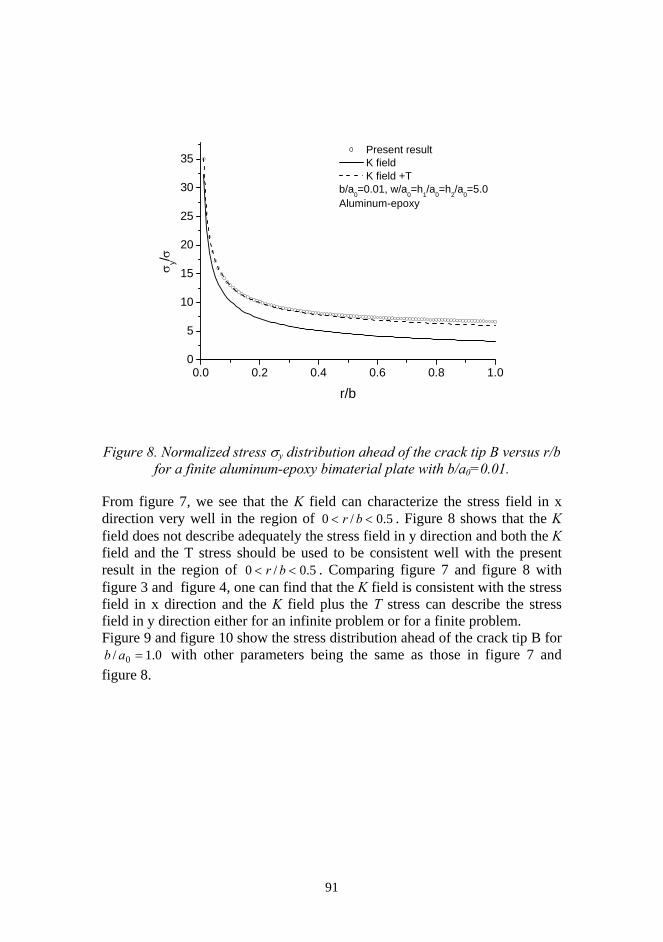
0.0 0.2 0.4 0.6 0.8 1.00

5

10

15

20

25

30

35σ y/σ

r/b

Present result K field K field +T

b/a0=0.01, w/a0=h1/a0=h2/a0=5.0Aluminum-epoxy

Figure 8. Normalized stress σy distribution ahead of the crack tip B versus r/b for a finite aluminum-epoxy bimaterial plate with b/a0=0.01.

From figure 7, we see that the K field can characterize the stress field in x direction very well in the region of 5.0/0 << br . Figure 8 shows that the K field does not describe adequately the stress field in y direction and both the K field and the T stress should be used to be consistent well with the present result in the region of 5.0/0 << br . Comparing figure 7 and figure 8 with figure 3 and figure 4, one can find that the K field is consistent with the stress field in x direction and the K field plus the T stress can describe the stress field in y direction either for an infinite problem or for a finite problem. Figure 9 and figure 10 show the stress distribution ahead of the crack tip B for

with other parameters being the same as those in figure 7 and figure 8.

0.1/ 0 =ab

91

0.0 0.2 0.4 0.6 0.8 1.00

1

2

3

4

5

6

7

8

σ x/σ

r/b

Present result K field

b/a0=1.0, w/a0=h1/a0=h2/a0=5.0Aluminum-epoxy

Figure 9. Normalized stress σx distribution ahead of the crack tip B versus r/b for a finite aluminum-epoxy bimaterial plate with b/a0=1.0.

0.0 0.2 0.4 0.6 0.8 1.00

1

2

3

4

5

6

7

8

σ y/σ

r/b

Present result K field K field+T

b/a0=1.0, w/a0=h1/a0=h2/a0=5.0Aluminum-epoxy

Figure 10. Normalized stress σy distribution ahead of the crack tip B versus r/b for a finite aluminum-epoxy bimaterial plate with b/a0=1.0.

92

From figure 9 and figure 10, we also see that the K field is consistent with the stress field in x direction and both the K field and the T stress should be used for the stress field in y direction in the region of 1.0/0 << br . Comparing figure 9 and figure 10 with figure 7 and figure 8, one can see that the distance

has a significant influence on the stress intensity factor so that the normalized stresses are quite different in figure 7, figure 8 and in figure 9 and figure 10. When the crack lies in a weaker material, the stress intensity factor decreases with increasing . Comparing figure 8 and figure 10, we can see that the T stress in y direction will become positive and tensile when the distance of crack tip B to the interface decreases, which means that the crack path is unstable and will change its advancing direction when the crack lies in a weaker material and the crack tip is near the interface. This result is consistent with that given by Ye, et al. [17].

b

b

When the crack lies in a stiffer material, the thing might be different from the case when the crack lies in a weaker material. We give the corresponding normalized stress distributions versus the normalized distance from crack tip B, , for the same edge length as those used in figure 9 and figure 10, but with different shear ratio.

br /

Figure 11 and figure 12 show the normalized stress distribution for epoxy-boron and the shear ratio is 007223.0/ 21 =µµ . Poisson's ratio of epoxy is

3.01 =ν and that of boron is 35.02 =ν and the normalized distance from the crack tip B to the interface is

b1.0/ 0 =ab . figure 13 and figure 14 show

the normalized stress distribution ahead of the crack tip B versus the normalized distance from the crack tip B, , for the case of with other parameters being the same as those used in figure 11 and figure 12.

br / 0.1/ 0 =ab

93

0.0 0.2 0.4 0.6 0.8 1.00

10

20

30

40

50

σ x/σ

r/b

Present result K field

b/a0=0.1, w/a0=h1/a0=h2/a0=5.0Epoxy-boron

Figure 11. Normalized stress σx distribution ahead of the crack tip B versus r/b for a finite aluminum-epoxy bimaterial plate with b/a0=0.1.

0.0 0.2 0.4 0.6 0.8 1.00

10

20

30

40

50

σ y/σ

r/b

Present result K field K field+T

b/a0=0.1, w/a0=h1/a0=h2/a0=5.0Epoxy-boron

Figure 12. Normalized stress σy distribution ahead of the crack tip B versus r/b for a finite aluminum-epoxy bimaterial plate with b/a0=0.1.

94

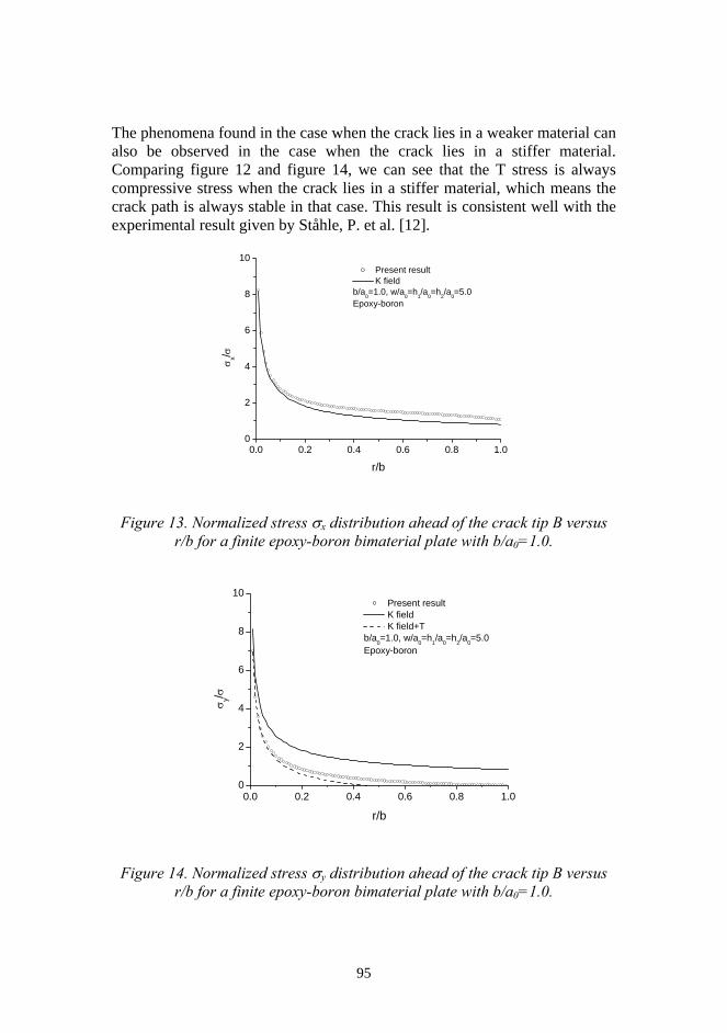
The phenomena found in the case when the crack lies in a weaker material can also be observed in the case when the crack lies in a stiffer material. Comparing figure 12 and figure 14, we can see that the T stress is always compressive stress when the crack lies in a stiffer material, which means the crack path is always stable in that case. This result is consistent well with the experimental result given by Ståhle, P. et al. [12].

0.0 0.2 0.4 0.6 0.8 1.00

2

4

6

8

10

σ x/σ

r/b

Present result K field

b/a0=1.0, w/a0=h1/a0=h2/a0=5.0Epoxy-boron

Figure 13. Normalized stress σx distribution ahead of the crack tip B versus r/b for a finite epoxy-boron bimaterial plate with b/a0=1.0.

0.0 0.2 0.4 0.6 0.8 1.00

2

4

6

8

10

σ y/σ

r/b

Present result K field K field+T

b/a0=1.0, w/a0=h1/a0=h2/a0=5.0Epoxy-boron

Figure 14. Normalized stress σy distribution ahead of the crack tip B versus r/b for a finite epoxy-boron bimaterial plate with b/a0=1.0.

95

All the above results are related with the effect of the distance and the crack 's position. For a finite problem, the scale of the sample must have an influence on the stress intensity factor. Now we consider the cases with different sample scales but with other parameters being the same.

b

Table 1 shows the normalized stress intensity factors 02 /)( aBK πσ for different ratios of the scale of the sample to the crack length versus different shear ratios, while the crack lies in a weaker material 2 and , 1.0/ 0 =ab

3.01 =ν . In Table 1, four kinds of samples with different scales are shown with different shear ratios, while the crack lengths are the same. From Table 1, one can see that the stress intensity factor will increase when the size of the sample decreases for the same shear ratio. The stress intensity factor is the smallest for the infinite problems. The stress intensity factor will decrease when the shear ratio of the upper material to the lower material increases for the same sample scale.

Table 1. 02 /)( aBK πσ for sample scales with the same crack length, when the crack lies in a weaker material ( 1.0/ 0 =ab , 3.01 =ν , 35.02 =ν ).

21 / µµ 1000.0 800.0 500.0 250.0 100.0 50.0 10.0 5.0 1.0

3/ 0 =aw3/ 01 =ah3/ 02 =ah

0.700 0.701 0.703 0.707 0.715 0.725 0.788 0.924 1.181

5/ 0 =aw5/ 01 =ah5/ 02 =ah

0.6670 0.6671 0.6672 0.6677 0.669 0.673 0.718 0.775 1.070

10/ 0 =aw10/ 01 =ah10/ 02 =ah 0.6440 0.6442 0.6446 0.6458 0.649 0.655 0.703 0.756 1.028

Infinite solid 0.6407 0.6408 0.6413 0.6426 0.6465 0.6529 0.7001 0.7517 1.014

96

Table 2 shows the normalized stress intensity factor 02 /)( aBK πσ for different ratios of the scale of the sample to the crack length versus different shear ratios, while the crack lies in a stiffer material 2 and , 1.0/ 0 =ab

35.01 =ν , 3.02 =ν . In table 2, four kinds of samples with different scales are shown with different shear ratios, while the crack lengths are the same. From Table 2, one can also see that the stress intensity factor will increase when the size of the sample decreases for the same shear ratio. The stress intensity factor is the smallest for the infinite problems. The stress intensity factor will increase when the shear ratio of the lower material to the upper material increases for the same sample scale.

Table 2. 02 /)( aBK πσ for sample scales with the same crack length, when the crack lies in a stiffer material ( 1.0/ 0 =ab , 35.01 =ν , 3.02 =ν ).

12 / µµ

1000.0 800.0 500.0 250.0 100.0 50.0 10.0 5.0 1.0

3/ 0 =aw3/ 01 =ah3/ 02 =ah 2.408 2.399 2.374 2.326 2.247 2.172 1.867 1.654 1.140

5/ 0 =aw5/ 01 =ah5/ 02 =ah 2.288 2.276 2.246 2.188 2.096 2.016 1.721 1.519 1.039

10/ 0 =aw10/ 01 =ah10/ 02 =ah

1.935 1.932 1.922 1.901 1.862 1.819 1.602 1.435 1.0

Infinite solid 1.755 1.754 1.752 1.747 1.730 1.704 1.536 1.393 0.985

From Table 1 and Table 2, one can find also that the normalized stress intensity factors are smaller than those for the homogeneous material, when the crack lies in a weaker material; they are larger than those for the homogeneous material, when the crack lies in a stiffer material. As for the case of an infinite solid with 0.1/ 21 =µµ in Tables 1 and 2, we can see the influence of Poisson's ratio. If 0.1/ 21 =νν , the normalized stress intensity factor is unity. Figure 15 and figure 16 give the normalized stress intensity factor versus the shear modulus ratio 21 / µµ with different normalized distances from the crack

97

tip B to the interface for two cases, when the crack lies in a weaker material and when the crack lies in a stiffer material. In figure 15, it is shown that when the normalized distance decreases, the stress intensity factor will decrease also. Figure 16 shows that when the normalized distance decreases, the stress intensity factor will increase.

0/ ab

0/ ab

1 10 100 10000.0

0.5

1.0

1.5

0.01

0.1

0.5

b/a0=1.0

Nor

mal

ized

stre

ss in

tens

ity fa

ctor

, K2(B

)/σ(π

a 0)1/2

µ1/µ2

w/a0=h

υ1=0.31/a

0=h

2/a

0=5.0

, υ2=0.35

Figure 15. Normalized stress intensity 02 /)(BK aπσ versus 21 / µµ for a finite bimaterial solid with different ratio of b , when the crack lies in a

weaker material. 0a/

0.0

0.5

1.0

1.5

2.0

2.5

1 10 100 1000

0.1

0.5

1.0

b/a0=2.0

Nor

mal

ized

stre

ss in

tens

ity fa

ctor

, K2(B

)/σ(π

a 0)1/2

µ2/µ

1

w/a0=h1/a0=h2/a0=5.0υ1=0.35, υ2=0.3

Figure 16. Normalized stress σy distribution ahead of the crack tip B versus r/b for a finite epoxy-boron bimaterial plate with b/a0=1.0.

98

3.2.2 The results for case II

Figure 17 and figure 18 show the stress distribution ahead of the crack tip B versus the normalized distance, , for aluminum-epoxy. Poisson's ratio of aluminum is

br /3.01 =ν and that of epoxy is 35.02 =ν . The shear ratio of the two

materials is 08.23/ 21 =µµ , which means the crack is in a weaker material. The normalized parameters are 0.5/ 0 =aw , 0.5// 0201 == ahah . The normalized distance between the crack tip B and the interface is . 01.0/ 0 =ab

0.0 0.2 0.4 0.6 0.8 1.00

5

10

15

20

25

30

35

σ x/σ

r/b

K field Present result

b/a0=0.01,w/a0=h1/a0=h2/a0=5.0Aluminum-epoxy

Figure17. Normalized stress xσ distribution ahead of the crack tip B versus

for a finite aluminum-epoxy bimaterial plate with br / 01.0/ 0 =ab .

From figure 17, we can see that the K field can characterize the stress field in x direction very well in the region of 5.0/0 << br . Figure 18 shows that the K field cannot describe adequately the stress field in y direction and both the K field and the T stress should be considered to be consistent well with the present result in the region of 5.0/0 << br . Comparing figure 17 and figure 18 with figure 3 and figure 4, one can see that the K field is consistent with the stress field in x direction and the K field plus the T stress can describe the stress field in y direction either for an infinite problem or for a finite problem. Comparing case I and case II, one can see that figure 17 is the same as figure 7.

99

0.0 0.2 0.4 0.6 0.8 1.00

5

10

15

20

25

30

35

40

σ y/σ

r/b

K field K field+T Present result

b/a0=0.01,w/a0=h1/a0=h2/a0=5.0Aluminum-epoxy

Figure 18. Normalized stress yσ distribution ahead of the crack tip B versus

for a finite aluminum-epoxy bimaterial plate with br / 01.0/ 0 =ab . Figure 19 and figure 20 show the stress distribution ahead of the crack tip B for with other parameters being the same as those in figure 7 and figure 8.

0.1/ 0 =ab

0.0 0.2 0.4 0.6 0.8 1.00

1

2

3

4

5

6

7

8

σ x/σ

r/b

K field Present result

b/a0=1.0,w/a0=h1/a0=h2/a0=5.0Aluminum-epoxy

Figure 19. Normalized stress xσ distribution ahead of the crack tip B versus

for a finite aluminum-epoxy bimaterial plate with br / 0.1/ 0 =ab .

100

0.0 0.2 0.4 0.6 0.8 1.00

1

2

3

4

5

6

7

8

σ y/σ

r/b

K field K field+T

b/a0=1.0,w/a

0=h

1/a

0=h

2/a

0=5.0

Aluminum-epoxy

Figure 20. Normalized stress yσ distribution ahead of the crack tip B versus

for a finite aluminum-epoxy bimaterial plate with br / 0.1/ 0 =ab .

From figure 19 and figure 20, we can also see that the K field is consistent with the stress field in x direction and the K field plus the T stress characterize the stress field in y direction, in the region of 1.0/0 << br . Comparing figure 19 and figure 20 with figure 17 and figure 18, one can see that the distance

has a significant influence on the stress intensity factor so that the normalized stresses are different in figure 17, figure 18 and in figure 19, figure 20, when the crack lies in a weaker material, the intensity decreases with increasing .

b

b When the crack lies in a stiffer material, the thing may be different from the case when the crack lies in the weaker material. We give the corresponding normalized stress distributions versus the normalized distance from crack tip B, , for the same sample scales as those used in figure 19 and figure 20, but with different shear ratio. Figure 21 and Figure 22 show the normalized stress distribution for epoxy-boron and the shear ratio is

br /

007223.0/ 21 =µµ . Poisson's ratio of epoxy is 3.01 =ν , that of boron is 35.02 =ν and the normalized distance from the crack tip B to the interface is . b 1.0/ 0 =ab

101

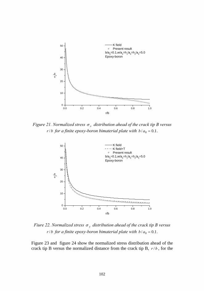
0.0 0.2 0.4 0.6 0.8 1.00

10

20

30

40

50

σ x/σ

r/b

K field Present result

b/a0=0.1,w/a0=h1/a0=h2/a0=5.0Epoxy-boron

Figure 21. Normalized stress xσ distribution ahead of the crack tip B versus

for a finite epoxy-boron bimaterial plate with br / 1.0/ 0 =ab .

0.0 0.2 0.4 0.6 0.8 1.00

10

20

30

40

50

σ y/σ

r/b

K field K field+T Present result

b/a0=0.1,w/a0=h1/a0=h2/a0=5.0Epoxy-boron

Fiure 22. Normalized stress yσ distribution ahead of the crack tip B versus

for a finite epoxy-boron bimaterial plate with br / 1.0/ 0 =ab .

Figure 23 and figure 24 show the normalized stress distribution ahead of the crack tip B versus the normalized distance from the crack tip B, , for the br /

102

case of 0.1/ 0 =ab and the other parameters are the same as those used in figure 21 and figure 22. The phenomena found in the case when the crack lies in a weaker material also can be observed in the case when the crack lies in a stiffer material.

0.0 0.2 0.4 0.6 0.8 1.00

2

4

6

8

10

σ x/σ

r/b

K field Present result

b/a0=1.0,w/a0=h1/a0=h2/a0=5.0Epoxy-boron

Figure 23. Normalized stress xσ distribution ahead of the crack tip B versus

for a finite epoxy-boron bimaterial plate with br / 0.1/ 0 =ab .

0.0 0.2 0.4 0.6 0.8 1.00

2

4

6

8

10

σ y/σ

r/b

K field K field+T Present result

b/a0=1.0,w/a0=h1/a0=h2/a0=5.0Epoxy-boron

Figure 24. Normalized stress yσ distribution ahead of the crack tip B versus

for a finite epoxy-boron bimaterial plate with br / 0.1/ 0 =ab .

103

Table 3 shows the normalized stress intensity factors 02 /)( aBK πσ for different ratios of the scale of the sample to the crack length versus different shear ratios, when the crack lies in a weaker material and 1.0/ 0 =ab , 3.01 =ν ,

35.02 =ν .

21 / µµ 1000.0 800.0 500.0 250.0 100.0 50.0 10.0 5.0 1.0

3/ 0 =aw3/ 01 =ah3/ 02 =ah

0.702 0.703 0.705 0.709 0.717 0.727 0.790 0.854 1.181

5/ 0 =aw5/ 01 =ah5/ 02 =ah

0.6687 0.6688 0.6689 0.6693 0.671 0.675 0.720 0.777 1.070

10/ 0 =aw10/ 01 =ah10/ 02 =ah

0.6456 0.6458 0.6462 0.6474 0.651 0.657 0.704 0.758 1.028

Table 3. 02 /)( aBK πσ for sample scales with the same crack length, when

the crack lies in a weaker material ( 1.0/ 0 =ab , 3.01 =ν , 35.02 =ν ) From Table 3, one can see that the stress intensity factor at crack tip point B will increase when the sample scale decreases for the same shear ratio. The stress intensity factor is the smallest for the infinite problems. The stress intensity factor at point B will decrease when the shear ratio of the upper material to the lower material increases for the same sample scale. Table 4 shows the normalized stress intensity factor 02 /)( aBK πσ for different ratios of the scale of the sample to the crack length versus different shear ratios, while the crack lies in a stiffer material and 1.0/ 0 =ab , 35.01 =ν ,

3.02 =ν . From Table 4, one can also see that the stress intensity factor at the crack tip point B will increase when the ratio of the sample scale to the crack length decreases for the same shear ratio. The stress intensity factor is the smallest for the infinite problems. The stress intensity factor at point B will increase when the shear ratio of the lower material to the upper material increases for the same sample scale.

104

12 / µµ

1000.0 800.0 500.0 250.0 100.0 50.0 10.0 5.0 1.0

3/ 0 =aw3/ 01 =ah3/ 02 =ah

2.604 2.602 2.593 2.571 2.512 2.426 2.002 1.727 1.138

5/ 0 =aw5/ 01 =ah5/ 02 =ah

2.343 2.341 2.333 2.314 2.262 2.187 1.818 1.574 1.039

10/ 0 =aw10/ 01 =ah10/ 02 =ah 1.955 1.954 1.950 1.940 1.912 1.870 1.633 1.453 1.0

Table 4. 02 /)( aBK πσ for sample scales with the same crack length, when

the crack lies in a stiffer material ( 1.0/ 0 =ab , 35.01 =ν , 3.02 =ν ) From Table 3 and Table 4, one can find also that the normalized stress intensity factors are smaller than those for the homogeneous material, when the crack lies in a weaker material; they are larger than those for the homogeneous material, when the crack lies in a stiffer material. As for the case of the infinite solid with 0.1/ 21 =µµ in Tables 3 and 4, we can see the effect of Poisson's ratio. If 0.1/ 21 =νν , the normalized stress intensity factor is unity. Figure 25 and figure 26 give the normalized stress intensity factor versus the shear ratio 21 / µµ with different normalized distances from the crack tip B to the interface for two cases, when the crack lies in a weaker material and when the crack lies in a stiffer material. In figure 25, when the normalized distance

decreases, the stress intensity factor will decrease also. figure 26 shows that when the normalized distance decreases, the stress intensity factor will increase.

0/ ab

0/ ab

105

1 10 100 10000.0

0.5

1.0

1.5

0.01

0.1

b/a0=1.0

K 2(B)/σ

(πa 0)1/

2

µ1/µ2

w/a0=h1/a0=h2/a0=5.0υ1=0.3,υ2=0.35

Figure 25. Normalized stress intensity 02 /)( aBK πσ versus 21 / µµ for a finite bimaterial solid with different ratio of , when the crack lies in a

weaker material. 0/ ab

1 10 100 10000.5

1.0

1.5

2.0

2.5

3.0

3.5

4.0

4.5

5.0

5.5

6.0

0.01

0.1

b/a0=1.0

K 2(B)/σ

(πa 0)1/

2

µ2/µ1

w/a0=h1/a0=h2/a0=5.0υ1=0.35,υ2=0.3

Figure 26. Normalized stress intensity 02 /)( aBK πσ versus 12 / µµ for a finite bimaterial solid with different ratio of , when the crack lies in a

stiffer material. 0/ ab

106

4 Conclusions

In the present paper, a crack perpendicular to the bimaterial interface of a finite solid is investigated analytically using the dislocation simulation approach and boundary collocation method.

A crack perpendicular to the bimaterial interface of an infinite solid is solved also. For both the finite and infinite solids, the normal stress xσ ahead of the crack tip, which is near the interface, is characterized by the K fields and the normal stress yσ is influenced by both the K field and the T stress in 5.0/0 << br region for 01.0/ 0 =ab ; when , the corresponding region is

0.1/ 0 =ab1.0/0 << br for both xσ and yσ .

As the crack approaches the interface, the parameter b becomes an important length scale, which characterizes the dominated zone of the K field and that of the K field plus the T stress field.

The stress intensity factor becomes larger when the sample scale decreases. In a finite solid, the stress intensity factor is larger than that in an infinite solid.

When the crack lies in a weak material, the stress intensity factor is smaller than that in the homogeneous material and the crack path is unstable when the crack tip is near the interface. When the crack lies in a stiffer material, the stress intensity factor is larger than that in the homogeneous material and the crack path is always stable with compressive T stress, which is consistent with the experimental results given by Ståhle, P. et al. [12], Ye, et al. [17] and Cotterell and Rice [18].

The stress distributions for the finite and infinite solids of bimaterial are very similar but with the different stress intensity factors.

Acknowledgements

The authors wish to acknowledge helpful discussions with Prof. Ståhle, P. of Malmö University, Sweden. This work is supported by NSF of China (No.10202023 and 10272103), Excellent Post-doctoral Research-Starting Fund of CAS and KJCX2-SW-L2 Fund of CAS.

107

References

1. Zak, A. R., Williams, M. L., Crack point singularities at a bimaterial interface. J. Appl. Mech., 1963, 30, 142-143.

2. Cook, T. S., Erdogan, F., Stress in bounded material with a crack

perpendicular to the interface. Int. J. Engng. Sciences, 1972, 10, 677-697. 3. Erdogan, F., Biricikoglu, B., Two bonded half plane with a crack through

the interface. Int. J. Engng. Sciences, 1973, 11, 745-766. 4. Bogy, D. B., On the plane elastic problem of a loaded crack terminating a

material interface. Int. J. Fract., 1971, 38, 911-918. 5. Wang, W. C., Chen, J. T., Theoretical and experimental re-examination of

a crack at a bimaterial interface. J. Strain Analysis, 1993, 28, 53-61. 6. Wang, T. C., Ståhle, P., Stress state in front of a crack perpendicular to

bimaterial interface. Eng. Fract. Mech., 1998a, 59, 471-485. 7. Wang, T. C., Ståhle, P., A crack perpendicular to and terminating at a

bimaterial interface. Acta Mech. Sinica, 1998b, 14(1), 27-36. 8. Lin, K. Y., Mar, J. W., Finite element analysis of stress intensity factors

for crack at a bimaterial interface. Int. J. Fract., 1976, 12, 521-531. 9. Meguid, S. A., Tan, M., Zhu, Z. H., Analysis of crack perpendicular to

bimaterial interface using a novel finite element. Int. J. Fract., 1995, 75, 1-25.

10. Chen, D. H., A crack normal to and terminating at a bimaterial interface.

Engng. Fract. Mech., 1994, 49, 517-523. 11. Suo, Z. G., Singularities interacting with interface and cracks. Int. J.

Solids Struct., 1989, 25, 1133-1142. 12. Ståhle, P., Jens, G., Delfin, P., Crack path in a weak elastic layer covering

a beam. Acta. Mech. Solida Sinica, 1995, 8, 579-583.

108

13. Leblond, J. B., Frelat, J., Crack kinking from an initially closed crack, Int. J. Solids Struct., 2000, 37, 1595-1614.

14. Chen, Y. Z., Closed form solutions of T-stress in plane elasticity crack

problems. Int. J, Solids Struct., 2000, 37, 1629-1637. 15. Dundurs, J., In mathematics of dislocation, edited by T. Mura, ASME,

New York, 1969, 70-115. 16. Gladwell, G. M. L., Contact problem in the classical theory of elasticity.

Sijthoff & Noordhoff, 1980, 61-64. 17. Ye, T., Suo, Z. and Evans, A. G., Thin film cracking and the roles of

substrate and interface. Int. J. Solids Structure, 1992, 29(21), 2639-2648. 18. Cotterell, B., Rice, J. R., Slightly curved or kinked cracks. Int. J. Fract.,

16, 155-169.

109

110

Paper E

A Crack Penetrating or Deflecting into an Interface in a

Thin Laminate

111

Paper E is submitted for publication as:

Kao-Walter, S., Ståhle, P. and Chen, S.H., A Crack Penetrating or Deflecting into an Interface in a Thin Laminate.

112

A Crack Penetrating or Deflecting into an Interface in a

Thin Laminate

S. Kao-Walter, P. Ståhle, S. H. Chen

Abstract

The crack tip driving force of a crack growing from a pre-crack that is perpendicular to and terminating at an interface between two materials is investigated by a linear fracture mechanics theory. The analysis is performed both for a crack penetrating the interface, growing straight ahead, and for a crack deflecting into the interface. The results from finite element calculations are compared with analytical results for asymptotically small crack extensions. The solution is found to be accurate even for fairly large amounts of crack growth. Based on this, the applicability of the analytical solution is made. By comparing the crack tip driving force of the deflected crack with that of the penetrating crack, it is shown how to control the path of the crack by choosing the adhesion of the interface relative to the material toughness.

113

1 Introduction

Thin aluminium foil and polymer laminate composites have proved their usefulness and high potential through many applications in various fields. In particular for packaging materials, components made from laminated materials are frequently designed to withstand extreme loads, not the least during the production. A better understanding of the failure mechanisms is useful for the design process and the production process of laminate with these components. An important task in the present work is to study in detail the fracture behavior of a crack situated in an aluminium foil (Al-foil) layer and terminating at the interface of this Al-foil and a low density polyethylene (LDPE) laminate. Many investigations of the interaction between a crack and an interface have been performed [1-8]. In one of the earliest works on the subject, Zak and Williams [9] used an eigenfunction expansion method to analyse the stress singularity at the tip of an infinite crack that is perpendicular to and terminating at the interface between two materials of an infinite body. Later, Wang and Ståhle [10, 11] used a dislocation simulation to extend the analysis to finite cracks and, recently, Chen et al. [12, 13] have studied a similar problem for a finite body. It was found that the finite boundaries have a significant influence on the stress distribution and the stress intensity factor, especially if the crack is situated in a weaker layer. While for a crack in a stiffer layer, the normal stress ahead of the crack tip and in a certain region near the crack tip can be characterized by the description of Zak and Williams. By applying a finite element method, [14-17] presented different analyses of stress intensity factors and energy release rates for cracks in different bi-materials. The present work applies a finite element method to analyze the crack tip driving force of a pre-crack that penetrates or deflects from the interface of an Al-foil/LDPE laminate. It is assumed that the pre-crack is located in a stiffer material and that the interface is perfectly bonded. For the case of deflecting, only the so-called double deflecting crack (cf. [8]) is considered.

114

2 Basic Equations

In [13], it has been shown that the singularity at the crack tip B (see figure 1) is of r-λ type for a crack perpendicular to and terminating at a bi-material interface. According to [13], this is so even in a finite solid in the region of 0<r/a0<1.0 for σx and 0<r/r/a0<0.5 for σy. According to Zak and Williams [9], the stress distribution in the vicinity of a tip of a crack that is perpendicular to a bi-material interface can be written:

σ ijo = ξo σ o ao / r( )λo fij(θ,α ,β ) . (2.1)

Here, σο is a remotely applied stress, ξo is a non-dimensional geometry dependent coefficient and λo is obtained as the largest root in the interval 0 ≤ λo < 1 of the following generating equation:

cos λoπ = 2(β −α )

1+ β(1− λo )2 + α + β 2

1− β 2. (2.2)

The angular functions fij are known (cf. [9]). Above, α and β are the two so called Dundurs’ parameters [18]:

α = Γ (κ2 +1) − (κ1 +1)Γ (κ2 +1) + (κ1 +1)

, β = Γ (κ2 −1) − (κ1 −1)Γ (κ2 +1) + (κ1 +1)

, (2.3)

where Γ = µ1 /µ2 , κ i = 3− 4ν i for the plane strain case and

κ i = (3−ν i ) /(1+ν i ) for the plane stress case. The material parameters νi and µi are Poisson’s ratio and the shear modulus of layer i where i=1 or 2.

For µ1 /µ2 → 0 , the expanded result of (2.2) gives (cf. [9])

λo = −1+ 0.88 µ1 / µ2 + O(µ1 / µ2 ) (2.4)

115

y

E D

h1

u

h22a0

B

ad

Figure 1. A crack perpendicular Here, the penetrating crack and th

A deflecting crack, a, along the inthe stress field

( ) ,(/ 2/101 αθσησ ε

iji

ij gra +∞=

where gij are known angular functiand η1 is a geometry dependent distance, a, along the interface, viakink should be the stress field giveas:

material 1 S1

material 2 S2

F

L

O

A

to the bimaterial interface e double deflecting crack a

ap and ad.

terface is, according to [8

), β ,

ons (cf. [9]), σ∞ is a remotconstant. If the crack pr a kink, the stress surroundn in (2.1). The the result is

116

x

C

u

o

eo

interface

ap

ad

f a finite solid. re illustrated by

], surrounded by

(2.5)

ly applied stress pagates a short

ing the tip of the readily obtained

( ) ( ) ),,(// 2/1

1 βαθσξσ ελij

iooij graaa o += . (2.6)

Here ξ1 is geometry dependent and

ε = 1

2ln 1+ β

1− β

⎛

⎝ ⎜

⎞

⎠ ⎟ .

(2.7)

Equation (2.6) is valid as long as the kink is fully embedded by the stress field (2.1). Similarily, the tip of a penetrating crack with the length, a, extending into the second material is surrounded by a stress field ( ) )(/ 2/1

2 θσησ ijij hra∞= , (2.8)

where η2 is an introduced geometry dependent constant. The angular functions hij are known as the angular functions of the Williams expansion. Again, as long as the tip of the crack is fully embedded in the stress field (2.1), the remote stress is identified as this stress field. Thus,

. (2.9) σij = ξ2 σo ao / a( )λo a / r( )1/ 2hij (θ )

Here ξ2 is a constant. The crack tip driving force, G, may be written as follows (cf. [8]):

00 2122

1

1

21 λλσξ

µν −−

= aaG oo . (2.10)

Here, ξ is a constant related to Dunders’ parameters. In the case when the crack deflects a distance a into the interface ξ = ξd(α, β). While in the case when the crack penetrates a length a into a homogenous material ξ = ξp(α, β), cf. [8].

117

One can also relate the crack tip driving force to the elastic energy release rate through [19]:

adPd

BG

2∆

= . (2.11)

Here ∆ is an applied constant displacement imposed on the edges of the specimen and B is assumed to be 1 mm for the present analysis. P is the resulting reaction force. After integrating over the full growth of the kink along the interface or equally over the full growth of the straight crack, (2.11) can be written as:

)(220 o

P

P

a PPPdadGo

−∆

=′∆=′ ∫∫ . (2.12)

Here the growth is in both cases considered as starting from the original crack with the length ao. By using (2.10), the left side of (2.12) becomes:

( )

)1(221 )1(2

1

221

0o

ooa oo aaadGλµ

ξσν λλ

−−

=′−

∫ . (2.13)

Hence, after using the relation (2.10), we finally obtain,

)()1(0PP

aG o −∆

−=

λ. (2.14)

This result is now based on the assumption that the stress fields described by (2.6) or alternatively (2.9) are valid. With (2.14) we are now equipped with a tool for evaluation of the asymptotic fields (2.9) and (2.6) with regard to their applicability for larger kinks and for cracks extending far into the second material. The limitation to the applicability of the asymptotic fields will reveal itself as a difference of G calculated using (2.10) and (2.14).

118

3 Finite Element Analysis

The general purposes finite element code [20] is used for the calculations. The finite element model with 7351 numbers of eight nodes plane strain elements with reduced integration was used. Near the crack tip, quadrilateral elements were applied (cf. [19]). The difference between the largest and smallest element size is 862. Due to the symmetry, only half of the geometry has been modeled. 3.1 Stress Distribution Along the Crack Tip

Finite element calculations have been performed using the same geometry and the boundary conditions as well as the same materials as in one of the cases analysed in [13]. As described in [13], a typical example of epoxy-boron in the case of plain strain was tested. Here, Poisson’s ratio of epoxy is υ1 = 0.35 and that of boron is υ2 = 0.3. The shear modulus ratio of the two materials is µ1/µ2 = 0.00722. The normalized parameters are w/ao = 5.0, h1/ao = h1/ao = 5.0. Here, h1 and h2 together equal the thickness of the laminate. The remote stress σo is applied at the boundary DOC as shown in figure 1.

Results of the stress distribution near the crack tip were compared to both the results from [13] as well as the results using equation (2.1). From (2.4), using given material data, one obtains the root λo ≈ 0.9252.

Figure 2 shows a log-log curve of σx/σo versus r/a. As it was found in [13], when the crack lies in the stiffer material, the normal stress ahead of the crack tip B can be characterized with high accuracy by equation (2.1) in the region of 0 < r/a < 1.0 for σx.

119

-2

-1,5

-1

-0,5

0

0,5

1

1,5

-2,5 -2 -1,5 -1 -0,5 0 0,5log(r/a 0 )

log( σ x / σ 0 )Ref.[13]FEMby Ref.[9]

Figure 2. Normalized stress σx distribution ahead of the crack tip B versus r/a0 for a finite epoxy/boron bimaterial.

3.2 Applying the FEM Model to Al-foil/LDPE Laminate

The finite element model was applied to analyse the laminate contain of Al-foil and LDPE. Here, a through pre-crack ao is placed in the Al-foil layer. A remote displacement uo was applied at the boundary DOC in figure 1. The shear modulus of the two materials is µ1 = 52.5 MPa and µ2 = 13200 MPa [21]. Poisson’s ratio of both Al-foil and LDPE is taken as ν1 = ν2 = 0.3 (cf. [22]). Thus, λo ≈ 0.9444 by (2.4). The stress distribution near the crack tip was calculated by the finite element method and compared to the analytical results by (2.1). The result of σx/σo versus r/a is shown in Figure 3. Again, good agreement is observed.

120

-4

-3,5

-3

-2,5

-2

-1,5

-1

-0,5

0-2,5 -2 -1,5 -1 -0,5 0 0,5

log(r/a 0 )

log( σ11 / σ0 )

FEMby Ref.[9]

Figure 3. Normalized stress σx distribution ahead of the crack tip B versus r/a0 for a finite Al-foil/LDPE bimaterial.

3.3 The Crack Tip Driving Force

The finite element model in 3.2 has then been modified. Here, the normalized geometry parameters are w / ao = 32.0 , h1 / ao = 8, h2 / ao = 2.0 . An element relaxation technique [16] is applied during the calculations of the crack tip driving force. The summation of the reaction force P0 at DOC is first calculated for the case that only a pre-crack existed. In the case of penetration, a crack with the length a is placed in material 1 (see figure 1). A series of reaction forces P can be obtained. Thus, the crack tip driving force, G, can be calculated for different crack lengths a by applying (2.14).

121

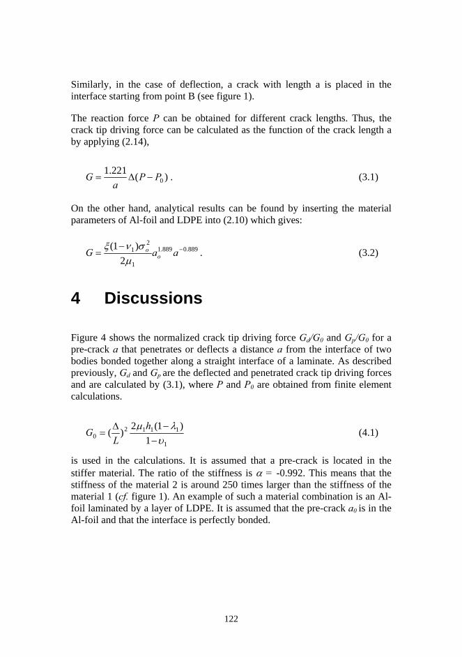
Similarly, in the case of deflection, a crack with length a is placed in the interface starting from point B (see figure 1).

The reaction force P can be obtained for different crack lengths. Thus, the crack tip driving force can be calculated as the function of the crack length a by applying (2.14),

)(221.10PP

aG −∆= . (3.1)

On the other hand, analytical results can be found by inserting the material parameters of Al-foil and LDPE into (2.10) which gives:

889.0889.1

1

21

2)1( −−

= aaG oo

µσνξ . (3.2)

4 Discussions

Figure 4 shows the normalized crack tip driving force Gd/G0 and Gp/G0 for a pre-crack a that penetrates or deflects a distance a from the interface of two bodies bonded together along a straight interface of a laminate. As described previously, Gd and Gp are the deflected and penetrated crack tip driving forces and are calculated by (3.1), where P and P0 are obtained from finite element calculations.

1

11120 1

)1(2)(υ

λµ−

−∆=

hL

G (4.1)

is used in the calculations. It is assumed that a pre-crack is located in the stiffer material. The ratio of the stiffness is α = -0.992. This means that the stiffness of the material 2 is around 250 times larger than the stiffness of the material 1 (cf. figure 1). An example of such a material combination is an Al-foil laminated by a layer of LDPE. It is assumed that the pre-crack a0 is in the Al-foil and that the interface is perfectly bonded.

122

0,00

1,00

2,00

3,00

4,00

5,00

-3 -2 -1 0 1log(a/a 0 )

log(G/G 0 )

FEM, deflectedanalytical, deflectedFEM, penetratedanalytical, penetrated

Figure 4. Normalized crack tip driving force G/G0 for deflected and penetrated crack versus normalized kink a/a0 for Al-foil/LDPE bimaterial loaded by a constant displacement. G0 is a crack tip driving force used as

reference as calculated by (4.1).

Also in figure 4, analytical results for asymptotically small crack extensions are shown. The results are calculated using the relation (3.2). These asymptotic solutions are found to be accurate even for fairly large amounts of crack growth (see figure 4). Figure 4 shows that even when the kink or the straight crack has extended to a length equal to the length of the original crack, the resulting crack tip driving force is rather close to the extrapolated result for an infinitesimal crack. At this point we are equipped with a possibility to calculate the toughness of the entire layer depending on the amount of crack kinking into the interface. With a known interface, the fracture toughness the length of the kink can be found in figure 4. Thus, the toughness of the entire laminate is h2 G2 + a Gi + h1 G1, where G1 is the fracture toughness of the LDPE, Gi that of the interface and G2 is the toughness of the Al-foil layer. The amount of crack growth in the interface at a given remote displacement can be found in figure 4. A

123

condition is, however, that the growing crack will set off along the interface. If not, a should be put to zero. Suppose now that the toughness of the interface is equal to Gic and the mode I toughness of the material is equal to Gc. As it has been discussed in [23], the crack will deflect into the interface if

p

d

c

ic

GG

GG

< . (4.2)

Figure 5 shows the ratio of the crack tip driving force for deflection and for penetration, Gd/Gp, by different α values. The results are compared to that from [8]. Good agreement can be found (see figure 5) when α<0. For Al-foil/LDPE laminate, α is equal to -0.992. It gives Gd/Gp=0.488. This means that the crack tip driving force for deflection from the straight path is around half of the value for penetration at the same crack length. This computation explains that the probability of crack deflection into the interface at increased displacement is large only if the toughness of the interface is less than half of the toughness of the LDPE layer. A full understanding of the final fracture of the LDPE layer requires further investigations because of the high ductility of this layer. The toughness of a ductile material tested using a large-scale geometry cannot easily be transferred to a very small specimen. Here, interaction with the Al-foil is expected since the linear extent of the plastic zone is of the same order of magnitude or larger than the thickness of the laminate layers (cf. [24]). A more detailed analysis requires modelling of the developed plastic deformation in the cross-section. The crack tip driving force for a very long crack in the interface has a lower limit which equals the elastic energy stored in the two layers of the laminate. For a lower limiting toughness of the interface the crack will, therefore, just spontaneously grow in the interface at a given load.

124

0

0,5

1

1,5

2

2,5

-1 -0,5 0 0,5 1α

Gd/Gp

FEMRef.[8]

Figure 5. The ratio of the crack tip driving force of a deflected crack to a double penetrated crack at the same crack length for different material

combinations.

5 Conclusions

The fracture of a layered laminate is modelled as a cross-section crack propagation. A finite element method is used to calculate driving forces for the crack tip depending on whether the crack will grow into the interface or will just continue straight ahead. The layer interface should be confined between a lower limit to ensure the spontaneous delamination of the entire structure and an upper limit over which there is no delamination or kinking at all. In the latter case, the fracture toughness of the laminate assumes a minimum value.

125

The results give guidance for the selection of ratio of material stiffness and the ratio of fracture toughness of the undamaged layer and the interface to maximize the toughness of the entire structure. Here an Al-foil and LDPE polymer laminate was chosen. For this material, the conclusion is that the toughness of the interface should be at least half of the toughness of the LDPE layer if benefit from the toughening delamination is desired. Large-scale plastic effects were not considered in this analysis. It is anticipated that such effects would limit the reliability of the results for accurate quantitative predictions.

Acknowledgements

This work was granted by Tetra Pak R&D AB, Tetra Pak Carton Ambient AB and the Print Research Program (T2F). The authors would like to thank the computer- and program support at Blekinge Institute of Technology and FEM-tech AB. Thanks also to Mr. Chong Li at Malmö University for assisting during the early stages of the finite element calculation.

References

1. Cook, T. S. and Erdogan, F., Stress in bounded material with a crack perpendicular to the interface. Int. J. Engng. Sciences, 1972, 10, 677-697.

2. Erdogan, F. and Biricikoglu, B., Two bonded half plane with a crack

through the interface. Int. J. Engng. Sciences, 1973, 11, 745-766. 3. Bogy, D. B., On the plane elastic problem of a loaded crack terminating a

material interface. Int. J. Fract., 1971, 38, 911-918. 4. Wang, W. C. and Chen, J. T., Theoretical and experimantal re-

examination of a crack at a bimaterial interface. J. Strain Analysis, 1993, 28, 53-61.

126

5. Chen, D. H., A crack normal to and terminating at a bimaterial interface.

Engng. Fract. Mech., 1994, 49, 517-523. 6. Suo, Z. G., Singularities interacting with interface and cracks. Int. J.

Solids Struct., 1989, 25, 1133-1142. 7. Ståhle, P., Jens, G.and Delfin, P., Crack path in a weak elastic layer

covering a beam. Acta Mech. Solida Sinica, 1995, 8, 579-583. 8. He, M. Y. Evans, Anthony and Hutchinson, J. W., Crack Deflection at an

Interface between Dissimilar Elastic Materials: role of residual stresses. Int. J. Solids and Structure, 1994, 31(24), 3443-3455.

9. Zak, A. R., Williams, M. L., Crack point singularities at a bimaterial

interface, J. Appl. Mech., 1963, 30,142-143. 10. Wang, T. C., Per, S., Stress state in front of a crack perpendicular to

bimaterial interface. Engng Fract. Mech., 1998a, 59, 471-485. 11. Wang, T. C., Per. S., A crack perpendicular to and terminating at a

bimaterial interface. Acta Mech. Sinica, 1998b, 14(1), 27-36. 12. Chen S. H., Wang, T. C. and Kao-Walter S., A crack perpendicular to the

bimaterial interface in finite solid. Int. J. Solids and Structure, 2003, 40, 2731-2755.

13. Chen, S. H., Wang, T. C. and Kao-Walter S., A crack perpendicular to

and terminating at the bimaterial interface in solid with finite body. Accepted by Acta Mech. Sinica, 2004.

14. Ståhle, P. and Shih, C.F., Cracking in thin films and substrates. Material

Research Society Symposium Proceeding, Vol.239, Boston, 1992. 15. Wäpping, D.,Gunnars,J. and Ståhle, P., Crack growth across a strength

mismatched bimaterial interface. Int. J. of Frac. 1998, 89, 223-243. 16. Delfin, P.,Gunnars and Ståhle, P., Effect of elastic mismatch on the

growth of a crack initially terminated at an interface in elastic plastic bimaterials. Fatigue Fract . Engng Mater. Struct. 1995, 18(10), 1201-1212.

127

17. Lin, K. Y., Mar, J. W., Finite element analysis of stress intensity factors for crack at a bimaterial interface. Int. J. Fract., 1976, 12, 521-531.

18. Dundurs, J., In Mathematics of Dislocation. edited by T. Mura, ASME,

New York, 1969, 70-115. 19. Anderson, T.L., Facture Mechanics, Fundamentals and Applications.

CRC Press LLC, ISBN: 0-8493-4260-0, Florida, USA, 1995. 20. ABAQUS, User’s manual, version 6.4, Hibbit, Karlsson and Sorenson,

ABAQUS, Inc. Printed in U.S.A., 2003. 21. Kao-Walter, S., Dahlström, J., Karlsson, T., and Magnusson, A., A study

of the relation between the mechanical properties and the adhesion level in a laminated packaging material. Mech. of Comp. Mat., 2004, 40(1), 43-52.

22. Tryding, J., In-plane fracture of paper. Ph.D-thesis, Report TVSM-1008,

ISSN: 0281-6679, Lund Institute of Technology, Lund, Sweden, 1996. 23. He, M. Y. and Hutchinson, J. W., Crack deflection at an interface

between dissimilar elastic materials. Int. J. Solids and Structure, 1989, 25(9), 1053-1067.

24. Kao-Walter, S. and Ståhle, P., Fracture behaviour of a thin Al-foil –

measuring and modelling of the fracture frocesses. Submitted for publication. (Parts of the results has been published in SPIE 3rd ICEM proceeding, ISBN: 0-8194-4261-5, Wu, X., Qin, Y., Fang, J., Ke, J. (eds.), Beijing, China, 2001, 253-256.).

128