8l. organization performing princeton university ctf rpr …
TRANSCRIPT

"WA &-pr, KEEP THIS COPY FOR REPRODUCTION PURPOSESForm Approved0MB No 0704-018
We 0avrgo hour Per r rse. "ldm etm o rev.e-"ng msrucl,ons er"l -s MC Za.Sure
ordaento *airrqt f .Ialcaaarters Services, Directorate for infoermatr,o Ocie'atior aric ;ecv. -tis~.' 12~ 15tC¶~Y jta~~ t' .onet~t ra. ~ a ert itersOffice of managemewnt and Budge. Paeerwor, Reducton Project (0704-0'SS) Wash.'gtcem CC 2ý^SC3
-... ORT DATE 3. REPORT TYPE ANC DATES COVERED
4. TITLE AND SUBTITLE 5pi 99 . FUNDING NUMBERS
Exploratory Data Analysis: Past, Present, and Future DA0-1G03
6. AUTHOR(S)
John W. Tukey
7. PERFORMING ORGANIZATION NAME(S) AND ADDRESS(ES) V"" ]k 8L. PERFORMING ORGANIZATION
Princeton University CTF RPR NME
Washington RoadFine Hll 'A
Princeton, NJ 08544-1000 K
9. SPONSORING /MONITORING AGENCY NAES N DRS(S 10. SPONSORING, MONITORING
U. S. Army Research Office AEC EOTNME
P. 0. Box 12211Research Triangle Park, N4C 27709-2211 1 ~2,97j-m
11. SUPPLEMENTARY NOTES
The view, opinions and/or findings contained in this report are those of theauthor(s) and should not be construed as an official Department of the Armyposition, policy, or decision, unless so designated by other documentation.
12a. DISTRIBUTION /AVAILABILITY STATEME NT 12b. DISTRIBUTION CODE
Approved for public release; distribution unlimited.
13. ABSTRACT (Maximum 200 words)
Abstract
The 1971-1977 early formulation of Exploratory Data Analysis, in terms of(a) results of some of its techniques and considerations which underlay, at Tar-ions depths, the choices realized in the books. The 1991-1995 development of
ýZk Exploratory Analysis of Vairiaince, described in its simplest (two-way table) formQ and barely sketched in general. Discussion of the changes in apparent philosophy
caused by the need to communicate more complicated things, notches, hints, thelikely impact on a revised edition of Exploratory Data Analysis 1977. Dreas-
C~J and tairgets for what might happen in 1996-2005, with emphasis on ExploratoryN Regression and the combined use of multiple description.
nmm.
I. SUBJECT TERMS iS. NUMBER OF PAGES
~ r 61- 16. PRICE CODE
F. SECURITY CLASSIFICATION 18. SECURITY CLASSIFICATION 19. SECURITY CLASSIFICATION 20. LIMITATION OF ABSTRACTOF REPORT j OF THIS PAGE OF ABSTRACT
UNCLASSIFIED I UNCLASSIFIED I UNCLASSIFIED __________
NSN 7540-01-280-5500 s~anda'd For"' 20Q 'Rev 2-89$Ores` oea bv AN%, Std Z39-'8

uI CLIMIR NOTICE
THIS DOCUMENT IS BEST
QUALITY AVAILABLE. TIHE COPY
FURNISHED TO DTIC CONTAIDA SIGNIFICANT NUMBER OF
PAGES WHICH DO NOT
REPRODUCE LEGIBLY.

/
Exploratory Data Analysis: Past, Present, and Future
John W. Tukey1
AcceýJoio For
Princeton University NTIS CRAM408 Fine Hall DTiC TAB
U. anrnounriced
W ashington R oad jt!--filc,,ofi .................................
Princeton, NJ 08544-1000 P- ....................Di t ib'ition I
Av,.ilability Codes
Avail nd, I orDist Special
Technical Report No. 302, (Series 2)Department of Statistics
Princeton University z-: * , i:j-• :
April 1993
'Prepared in connection with research at Princeton University supported by theArmy Research Office, Durham DAAL03-91-G-0138, and facilitated by the Alfred P.
Sloan Foundation. Presented at University of Maryland - Year of Data: miniserieson Statistical Data, April 20-22, 1993.

ii
Exploratory Data Analysis: Past, Present, and Future
John W. 2ke9
Technical Report No. 302Princeton University, 408 Fine Hall, Wauhington Road, Princeton, NJ 08544-1000
Abstract
The 1971-1977 early formulation of Exploratory Data Analysis, in terms of(a) results of some of its techniques and considerations which underlay, at var-ious depths, the choices realized in the books. The 1991-1995 development ofExploratory Analysis of Variance, described in its simplest (two-way table) formand barely sketched in general. Discussion of the changes in apparent philosophycaused by the need to communicate more complicated things, notches, hints, thelikely impact on a revised edition of Exploratory Data Analysis 1977. Dreamsand targets for what might happen in 1996-2005, with emphasis on ExploratoryRegression and the combined use of multiple description.
'Prepared in part in connection with research a Princeton University, supported bythe Army Research Office, Durham, DAAL03-91-G-0138, and facilitated by the AlfredP. Sloan Foundation. Presented at University of Maryland - Year of Data: miniserieson statistical Data, April 20-22, 1993.

Exploratory Data Analysis: Past, Present, and Future ii
Contents
Abstract i
Introduction 1
A Exploratory Data Analysis, 1971-1977 1ambiance ........................................... 2interrelation ......................................... 4the seventies ......................................... 5
1 Principles, overt or tacit, in EDA(71 to 77) 5most visible ......... .................................. 5relatively explicit ...................................... 6more explicit ....................................... 7procedure-orientation vs theory-orientation ..................... 7
2 Techniques, overt or tacitly, in EDA71 and EDA77 9stem-and-leaf displays .................................. 9
exhibits "10 of Chapter 1" and "B of exhibit 4 of chapter 3" . . . 10a,bletter and outside values ....... ........................... 10schematic plots ........ ................................ 11
"exhibit 8 of Chapter 2" .............................. 11a"exhibit 6 of Chapter 2" ............................. 11b
reexpression. ........................................... 11"exhibit 12 of Chapter 3". ............................ 11c"exhibit 18 of Chapter 3" ............................. 12a"exhibit 19 of Chapter 3" ............................. 12b
straightening curves ...................................... 12"exhibit 21 of Chapter 6" ............................. 12c
two-way tables ........ ................................ 12"exhibit 1 of Chapter 10" ............................. 13a"exhibit 7 of Chapter 10" ........................... 14a"exhibit 8 of Chapter 10" ............................. 14b
plus-one fits; diagnostic plots ....... ........................ 14"exhibit 10 of Chapter 10" .......................... 15a"exhibits 3 and 4 of Chapter 12 ....................... 15b
resistant smoothing ...................................... 16"exhibit 1 of Chapter 7'.... . ......................... 16a"exhibit 6 of Chapter 7". .............................. 16b

Exploratory Data Analysis: Past, Present, and Future ii
"exhibit 2 of Chapter 15" ............................. 17adistributions in bins ..................................... 18
"exhibit 5 of Chapter 17" ............................. 18adistribution of counts ........ ............................. 18
"exhibit 10 of Chapter 17" ............................ 18bextreme J-shaped distributions ...... ....................... 18
"exhibit 4 of Chapter 18" ............................. 19a"exhibit 7 of Chapter 18" ............................. 19b"exhibit 8 of Chapter 18" ............................. 19c
3 Selected aphorisms 20close .......... ...................................... 21
References 22
B Exploratory Data Analysis, 1991-1994 23
1 What has changed in technique? 23re-expression. ......................................... 24alternative medians ........ .............................. 27rootograms ........ .................................. 28
Figure 1: Histogram ....... ......................... 28aFigure 2: Rootogram ................................ 28aFigure 3: Hanging Rootogram .......................... 28bFigure 4: Suspended Rootogram ........................ 28b
other changes in EDA (1977) ................................ 28
2 Exploratory analysis of variance - - two-way tables as an initiation 29comparison ......... .................................. 29
Exhibit 1: A conceptual look at two analyses of the same 3 x 5data set .......... .................................... 30a
Exhibit 2: Hypothetical example of two-way analysis ....... .. 32aExhibit 3: Hypothetical example (continued) ............... 32bExhibit 4: Hypothetical example (continued) ............... 32c
3 Exploratory analysis of variance, the general factorial case 33important aspects touched upon ............................. 34literature and work in progress ............................... 34conclusions ......... .................................. 35
Exhibit 5: The basic rationale of notches .................. 36aExhibit 6: An example of a notch display for 41 versions ..... .36b

Exploratory Data Analysis: Past, Present, and Future iv
some of the novelties ........ ............................. 36hints .......... ...................................... 36
Exhibit 7: Novel aspects of exploratory analysis of variance, 1 . 37Exhibit 8: Novel aspects of exploratory analysis of variance, 2 38Exhibit 9: Novel aspects of exploratory analysis of variance, 3 . 39Exhibit 10: Novel aspects of exploratory analysis of variance, 4 40Exhibit 11: Novel aspects of exploratory analysis of variance, 5 41Exhibit 12: A set of guidezones for guiding mention of differ-
ences in terms of what fraction of the difference that is bare worth aconclusion ............................................. 42a
Exhibit 13: Extremes of hint Zone A - - mention likely - - unlesslist too long ......... .................................. 43a
Exhibit 14: Extremes of hint Zone B - - mention reasonable - -unless list too long ........ .............................. 43b
Exhibit 15: Extremes of hint Zone C - - mention unlikely, butpossible .......... .................................... 43c
4 Generalities 43
References 44
C Exploratory Data Analysis, 1995-2005 45
1 Regression 45exploratory regression: description or prediction? . . .. . . . . . . . . . .. . . 46
2 Enhanced techniques for exploratory regression 48diagnosing for re-expression ....... ......................... 48clarifying how we think about re-expressions ..................... 49exploratory path regression ................................. 50robust regression ........ ............................... 50non-data-directed and triskeletally fitted composites ................ 51exploring multiple answers ................................. 52graphical techniques for two or more alternative regression fits ...... .. 53looking harder at "stopping rules' . . . . .. . . . . . . . . . . . . . . . . .. . . . . 54
3 Unbalanced exploratory analysis of variance 54
4 Generalities 55parallel alternatives .................................. 55guidance about common pairs of analyses ........................ 56
iNS Ill i i0

v
Exploratory Data Analysis: Past, Present, and Future
how are parallel analysis best combined ........................ 56
required re-orientations ....... ........................... 56
strategy guidance ............ ....................... 57
bringing hints into the fabric ............ ................ 57
procedure orientation ...................................
61
References

Exploratory Data Analysis, 1971-1977 1
Introduction
The three lectures that follow this introduction, were written for and presented at a
miniseries on Statistical Data that was part of the "Year of Datat program sponsored
by CHPS (Campus History and Philosophy of Science Program) at the University of
Maryland, College Park. The whole program involved more than 50 lectures.
These three talks were intended to provide material of interest for a diverse audience,
from those who might like an idea of what Exploratory Data Analysis (EDA) was about,
to those whose interest focused on the philosophy that underlay, underlies, and will
underlie EDA at various stages of EDA's development.
PART AExploratory Data Analysis, 1971-1977
Exploratory data analysis seemed new to most readers or auditors, but to me it was
really a somewhat more organized form - - with better or unfamiliar graphical devices
- - of what subject-matter analysts were accustomed to do. Most of the novelty lay in:
"* organization of a collection of tools and approaches,
"* new or unfamiliar tools,
"* simple arithmetic,
"• procedures legitimized by showing that they worked rather than by being derived
from a "model",
"* recognition that much that was useful in the analysis of data could be done without
any mention of probability,
Exploratory Data Analysis, 1971-1977 2
"* willingness to notice some things that had in fact happened by chance alongside
things that had a continuing existence - - willingness not to require considering
only conclusions (for significance or confidence),
"* emphasis on
data = fit + residual
where the fit is admittedly incomplete - - not just uncertain,
"* emphasis on stripping off layer after layer of what could be described.
We turn to the background of exploratory data analysis, before discussing its prin-
ciples and techniques.
* ambiance *
The environment of attitude being pushed by statisticians at the time that EDA was
being developed was rigid, protective, and optimistic. One was supposed to be led to the
procedures to be used by deriving them from a model, which means from assumptions.
The true applicability of the assumptions was hardly ever in question; if the assumptions
were questioned, it was ordinarily in the mode of "can one show they must be wrong"
by attaining significance on some test.
We need to ask what purposes were served by such a distorted picture of the process
of choosing what to do. Two considerations stand out, one for the technique maker or
teacher, the other for the technique user:

Exploratory Data Analysis, 1971-1977 3
"* A mathematically minded technique purveyor can check the detailed logic and
verify that a particular procedure does optimize an assumed criterion, given the
assumptions of the model - - whether or not the procedure works well in real
world can then, by those concerned with the abstract method rather than its use,
be forgotten about!
"* So long as there is only one standard model, only one procedure, giving only one
answer as optimal, this uniqueness tends to avoid conflict about what the data at
hand says, or means.
The first allows mathematicians, whether called mathematicians or mathematical
statisticians, to be almost happy teaching "statistics" (some may even think they are
teaching how to analyze data). The second has real, though essentially administrative,
rather than technical or scientific, advantages at the price of, at least occasionally, leading
to inadequate analyses of certain data sets.
Further, one was supposed to tailor the model to what could be at least estimated
from the data. It would have been - - and still is, too often, today - - thought improper
to include in the model pieces that were known to have a real and separate existence, if
the nature of the data precluded at least estimatir S, however roughly, the contribution of
these separate pieces. In a two-way table of responses, for instance, with one observation
per cell, one's model had to include "interaction" or "error" but not both - - although
it was widely understood that both were essentially always present.
To make data analysis look even more like mathematics or logic, rather than like
Chamberlin's science ("Science is the holding of multiple working hypotheses"), the

Exploratory Data Analysis, 1971-1977 4
results of analysis were supposed to consist of significant results and non-significant
results:
"* things "significant" perhaps "at 5%" were to be taken as established,
"* those "nonsignificant" were to be taken as "zero" or as "alj exactly alike".
Confdence intervals were accepted as kosher, but usually used quite sparingly, pre-
sumably because it causes pain to both mathematicians and investigators to recognize,
explicitly, the presence of uncertainty.
* interrelation *
The view I have held, so far back as I can remember, is that we need both exploratory
and confirmatory data analysis. Truly confirmatory calls for data collected (or mined)
after the question(s) have been clearly formulated. The process of formulating the %.ies-
tion and planning the data acquisition will, often, have to depend on exploratory analyses
of previous data. This is not the only instance of cooperation between exploratory and
confirmatory, but it is probably the most pervasive one.
There are extensive important instances where the main analysis of data collected for
a purpose is exclusively confirmatory. Controlled clinical trials, as usually conducted,
are only one instance. But it will often be foolish not to parallel the main (confirmatory)
analysis, which is often, as it needs to be, carefully focused on one or two questions, with
a parallel exploratory analysis looking around for suggestions that ought to infi. .uce the
planning of both the conduct and the analysis of the next experiment.
Neither exploratory or confirmatory alone, will meet our needs in subject-matter

Exploratory Data Analysis, 1971-1977 5
areas where the collection of data can be planted to respond to a question. (Elsewhere
we may only be able to do exploratory.)
* the seventies •
Writing the limited preliminary edition of Exploraotory Data Analysi was a necessary
relief from finding myself a part-time (at the University) chairman of a new university
Department of Statistics, as was teaching from it to a mixed class of undergraduates.
It (EDA71) ended up as containing about twice as much material as the First Edition
(EDA77) contained when it appeared several years later. While infelicities and errors
are my responsibility alone, EDA77 is clearer and more understandable because of the
yeoman editorial efforts of Frederick Mosteller.
1 Principles, overt or tacit, in EDA(71 to 77)
We will find it convenient to discuss the ideas, concepts, and principles that underlie
EDA71 and EDA77 by starting with the most visible and moving toward the less visible.
. most visible *
Probably the most visible aspects of EDA71/EDA77 were:
"* unfamiliar or new techniques, which we shall illustrate shortly,
"* emphasis on seeing results - - graphically, or numerically,
"* emphasis on simple arithmetic (almost all divisions, for example, are divisions by
2),
"* no probability, either formal, or informal,
Exploratory Data Analysis, 1971-1977 6
* emphasis on
data = fit + residuals
9 emphasis on successively better fits, and on the incompleteness of all fits.
Emphasis on seeing results contrasts strongly with classical confirmatory's emphasis
on s3gnificant vs. nonsignificant, and substantially supplements modern confirmatory's
emphasis on confidence statements (often made in the light of multiplicity). If our
procedures are to be supported by a history of situations where they have worked well,
we need to have looked at many data sets in ways for which we can have some idea how
well the procedures have worked. As a minimum, we need answers in context. Almost
always this means being able to look at the results in some sort of context. Doing this, in
turn, usually means either well-planned graphical presentation, or well-planned tables,
or both.
* relatively explicit *
What was relatively explicit in EDA71/EDA77 included:
"* a flexible attitude of mind - - illustrated by a substantial emphasis on reexpression
(it may not suiffce to analyze the numbers we were given, it may be wiser to analyze
their square roots, logs or reciprocals, for instance),
"* wherever possible, flexible techniques - - for instance analyzing two-way tables
both by means and by medians,
"* willingness to find some happenchance phenomena, as well as happiness in finding
phenomena with some continuing reality,

Exploratory Data Analysis, 1971-1977 7
"* description of structure, layer by layer, each description incomplete, calling for
further inquiry hopefully followed by further fitting,
"* introduction of robust smoothing, both for equispaced sequences and for further
diagnosis,
"* special plots, inciuding the diagnostic plot and plots for row-PLUS-column fits.
* more implicit
Here we ought to call attention to:
"* procedure-oriented processes rather than theory-oriented ones,
"* things that can be tried, rather than things tbat "must" be done,
"* appearances need not be significant to be relevant and worth some attention,
"* techniques of, say, Ž 50% efficiency in each of a wide variety of circumstances are
ee often satisfactory,
so better for general use than techniques which have 100% efficiency, but only
for a very narrow bouquet of situations,
"* hanging and suspended rootograms, to which we shall return.
* procedure-orientations vs theory-orientation *
This point was implicit in the structure and content of EDA71 and EDA77, though
we should not be surprised if many readers missed it entirely. Theory, for your speaker, is
now to be explicated as that which is based on a set of assumptions. This means that the
*
Exploratory Data Analysis, 1971-1977 8
results of experimental sampling - - or of more sophisticated forms of simulation, such
as Monte Carlo - - while they are fuzzy to the extent of sampling fluctuations, are just
as much theory as the results of formula manipulations and the application of relevant
mathematical theorems. This is so because the simulations are designed to simulate
specific situations, whose description automatically takes the form of assumptions.
The recognitions and "assumptions" familiar to the mathematical statistician, when
viewed from data analysis, fall into at best three categories, as it is easy to illustrate for
the case of fitting a straight line, namely:
"* a recognition that describing, incompletely, some of the (incomplete) dependence
of y on z by a straight line may be useful,
"* an assumption that the observed y's deviate from a straight line in a well-behaved
(e.g. uncorrelated, mean zero) way,
"* an assumption that the joint distribution of the y's takes a specified form, usually
Gaussian.
Checking either of the latter two statements, the "assumptions" is enough harder than
checking the first, the "recognition" as to be essentially never done. Procedure orienta-
tion tells us not to rely heavily upon the uncheckable.
Classical least-squares is theory-oriented. If we are fitting/summarizing a collection
of z's and each data point has equal variance, and each pair has equal covariance, then:
"* among linear cormbinations, the arithmetic mean gives results of minimum variance,
"* if the individual data points follow Gaussian distributions, then, among all sum-
maries that commute with translation, the arithmetic mean is best.

Exploratory Data Analysis, 1971-1977 9
These are strong theory-oriented reasons supporting the arithmetic mean. But are they
enough?
At the other extreme, the median obviously works reasonably well in a wide variety
of situations. This is a strong procedure-oriented reason supporting the medium. As
is the existence of distributions of infinite variance, but not otherwise pathological, for
which the arithmetic mean fails dismally, though the median performs quite well.
So much for philosophy, attitudes and orientation, it is time we turned toward
techniques, particularly graphical techniques.
2 Techniques, overt or tacitly, in EDA71 and EDA77
Rather than follow the order of presentation in EDA itself, we plan to focus on what
seem to be the most used techniques, simplest first.
*r stem-and-leaf displays *
A simple improvement on an ancient graphic display of distribution information,
where 1 value of 36, 1 of 52, and 1 of 89 would classically been shown as
23 x45 x678 x9
takes account of the next digit in the value, writing

Exploratory Data Analysis, 1971-1977 10
23 645 2678 99
instead. Exhibits "10 of Chapter 1" and "B of exhibit 4 of Chapter 3" show two
examples from EDA77.
Among the advantages of stem-and-leaf displays are:
* simplicity enough to make them the fastest way to record batches,
* enough detail to serve as a basis for almost any desired computation,
* visual impact comparable with a histogram.
* letter and outside values *
There are often needs for summarizing a batch in more detail than one number (but
many fewer than all). In an EDA context, the individual summaries need to be simply
defined and easy to use, and to function well over a variety of batch shapes. Emphasis
on order statistics - - e.g. medians and extremes - - was thus almost automatic. Which
intermediate order statistics? The simple answer was those defined by halving: the
median halves the batch, the hinges (or fourths) halve each of these halves, the eighths
halve the outer quarters, and so on. The detailed definition for halving was chosen to
be convenient for small batches; thus a batch of five is made up of 2 extremes, 2 hinges,
and 1 median. Half-integer order statistics - - means of two adjacent order statistics -
- are permitted, but additional fractionation is excluded.

10a
exhibit 10 of chapter 1: state heights
The heights of the highest points In each state
A) STEM-and-LEAF--unit 100 feet(#)
0* 43588 Del, Fla, La, Miss, RI (5)1 237886 (6)2 484030 (6)3 45526 (5)4* 80149 (5)5 34307 (5)6 376 (3)7 2 S. Dak (1)8* 8 Texas (1)9
1011 2 Oregon (1)12* 768 (3)13 81258 (5)14 544 Calif, Colo, Wash (3)1516*17181920* 3 Alaska (1)
(50,1)

exhibit 4 of chapter 3 (continued) 10b
B) BACK-to-BACK STEM-and-LEAF--leaves sorted, as wellMichigan Mississippi
Benzie 2 3.Leelanau, Arewac 75 - 8 TateCharlevoix 1 4. 0001111112222223344
9988665 - 5555666788994443221100 5. 001124
88877777777776666666666655 - 5777788999994110 6* 112444865 - 588899
422110 7* 00122333465 - 56678
3221 8! 033866 * 8 Hinds110 9. 24 Bolivar, Yazoo
6 °'
331 101
Delta, Gogebic 8 11.
Iron 00 12.
Ontonagon 2 131
14*0
Chippewa 151
"16
17*
Marquette 4 18l
(83, check (82, check)

Exploratory Data Analysis, 1971-1977 11
The values of the hinges, and their separation, the hinge spread, allow the definition
of fences (1.5 hingespreads outside the hinges) and outer fences (3 hingespreads outside
the hinges). (These were differently defined in EDAT1, but the performance of the outer
definitions indicated a change.) Values outside an outer fence are "far out', those outside
only a fence is "outside". (The value inside but closest to a fence is graphically usefully
and called "adjacent".)
Thinking of hinges as always at the 25% points of a Gaussian population gives rise
to unmet expectations about how few "far out" or "outside" values we ought to expect
in "nice" data. (See Hoaglin, Iglewicz and Tukey 1986m for information about what
actually happens in random sarnples from Gaussian istributions, as well as distributions
with more stretched tails.)
* schematic plots
With this much machinery, it is time to turn to pictures. "exhibit 8 of Chapter
2" shows such a plot, with median, hinges, and adjacent values shown by lines, while
outside and far-out values are labelled. An earlier form, that does not show adjacent
values is represented by "exhibit 6 of chapter 2" which shows the effectiveness of such
plots in comparison of batches.
Notches in box plots escape 1971-77 by a year (McGill, Tukey and Larson 1978a).
* reexpression *
The simplest use of reexpression is to avoid (or reduce) unsymmetrical tailing off of
the values to be analyzed. "exhibit 12 of Chapter 3" shows how looking at alternative
schematic plots can show which one of a few alternatives to prefer.

Ila
exhibit 8 of chapter 2: county areas
Michigan counties, orea in m?
A) SCHEMATIC PLOT
Arca(S q Are m; Its)
0MAREu•TTE
o C•iPPErWA
1600
Irw. * • •cho,Icraft
G,,gcbic)- 'T-•Iro
• I000- It
SoI
I
--- I

l1b
exhibit 6 of chapter 2: various heights
Box-and-whisker plots with end values identified
A) HEIGHTS of 50 STATES B) HEIGHTS of 219 VOLCANOS
Height
(fe t)
Ala~ka. 20E,000 Gjs jar.*tGellatiripa
California 15, 000
Cdoradc * 0 washinfitoRaw3; i V ¢YOM min
l 10,000
Deaaare loida lsaWa Anak Krakatau
I lr a0 1hNv

Ile
exhibit 12 of chapter 3: volcano heights
leights of 219 volcanoes, using three different expressions (schematic plots; forurther identification so# exhibit 6 of chapter 2)
tIsht lHr;ght ye;ght(r, (I°gi) (r,,ts)
4 -
K; *,,PC*ITI- IG;°TM I0
II_11a Nova
CiN6
,• ZZZ]WZ7 N7Zj

Exploratory Data Analysis, 1971-1977 12
In EDA77, reexpression of amounts is confined to integer and half-integer powers of
the raw numbers, with inevitable major emphasis on square roots and logs and lesser
emphasis on raw values and (negative) reciprocals. "exhibit 18 of Chapter 3" of EDA77
shows, on a matched basis, powers of 3, 2, 1, 0, -1, -2 and 3. 'exhibit 19 of Chapter
3" shows, also on a matched basis, powers 1, 1/2, 0 (represented by logs), -1/2 and -1
in such a way as to clarify the role of logs as the zero power.
* straightening curves *
Here there is little novel, except possibly the emphasis on selecting 3 points and
straightening them, and the rule of thumb "move on the ladder of expressions in the
direction in which the curve bulges" as explained by "exhibit 21 of Chipter 6".
* two-way tables *
It is now time to jump ahead in the book and pick up material that might have
appeared immediately after the first six chapters, but did not.
Our concern now is with two-way tables of responses, a situation where:
o there are two factorS - - usually "treatments" or "circumstances",
* each factor has two or more versions,
* for each pair of versions (or, perhaps, nearly every pair) there is a value of the
response.
The first example we look at will have:
* one factor: places in Arizona, with versions; Flagstaff, Phoenix and Yuma,

exhibit I8 of chapter 3: powers and logs12
The "shape" of simple functions of x
(Expressions of Vie form A + 8 - x), with A and 8 chosen to make the result tangentto x - 1 at x =1.) Labels give Ax). For A and 8 see below.
log Ar
lot~~~ I/ere I(
0t+
2. S01 log" Sg
f 0 /jr%) -1/,W&
.5 1.

12b
exhibit 19 of chapter 3: powers and logs
Logs and the usual powers
Re-• e~i•7 /;"lot.
~ J7 ieg
--i
jEr
SPlo~t ed " Labelled!
-Z + z~q" M
2.303 I.g, loL+ z(- i/J-, -I I/X,
-V rjr -11.N
I I _ I I I I . .
0.3 0.4 05S 0.7 I 1.5 2 3 4

12c
exhibit 21 of chapter 6: indicated behavior
How to move for each variable separately;the four cases of curve shape
OR toward eytc, et. tuwarý y', y', etc. ORtowarg tw.ard
.etc.
t o w s. t fw.4rd
etC. e'tc.OR toward lot Y)-Iuetc. tovrard log YO.

Exploratory Data Analysis, 1971-1977 13
* another factor: months of the calendar; with versions July to January,
9 response: mean monthly temperature (from U. S. Weather Bureau).
"exhibit 1 of Chapter 10" of EDA77 shows the data and the first stages of breaking each
data value up into 4 parts:
"* a common value, here 70.8*F, applying to all values,
e a row (month) effect, here between 19.1 and -21.1, depending on month but the
same for all places,
"* a column (place) effect; here between -29.7 and 5.6, depending on place, but the
same for all months,
"* residuals; here between -1.0 and 1.9, one for each input value.
The NW corner of the original table, Flagstaff in July, started as 65.2 and broke down
as
0 + 19 + (-24.7) + 70.8 = 65.2.
This was a ROW-plus-COLUMN analysis, and full of + signs. The corresponding
ROW-plus-COLUMN fit is the sum of ROW, COLUMN and COMMON contributions
and can be calculated, sometimes most easily, from
FIT = DATA - RESIDUALS
a transposed form of the important general relation
DATA = FIT + RESIDUALS

13a
exhibit I of chapter 10: Arizona temperatures
Two-way residuals (cooling down Arizona)
A) The MEAN MONTHLY TEMPERATURES--in "F
Flagstaff Phoenix Yuma
July 65.2 90.1 94.6Aug 63.4 88.3 93.7Sept 57.0 82.7 88.3Oct 46.1 70.8 76.4Nov 35.8 58.4 64.2Dec 28.4 52.1 57.1Jan 25.3 49.7 55.3
B) FITTED PLACE VALUES, their RESIDUALS--and some MONTH MEDIANS
fit 46.1 70.8 76.4 70.8
July 19.1 19.3 18.2 19.1Aug 17.3 17.5 17.3 17.3Sept 10.9 11.9 11.9 11.9Oct 0 0 0 0Nov -10.3 -12.4 -12.2 -12.2Dec -17.7 -18.7 -19.3 -18.7Jan -20.8 -21.1 -21.1 -21.1
C) The MEDIANS of panel B taken out; SECOND RESIDUALS
eff70.8 -24.7 0 5.6
July 19.1 0 .2 -. 9Aug 17.3 0 .2 0Sept 11.9 -1.0 0 0Oct 0 0 0 0Nov -12.2 1.9 -. 2 0Dec -18.7 1.0 0 -. 6Jan -21.1 .3 0 0
Note the appearance of "off" for "effect," used for values obtained from repeatedfitting, whether or not these are fits to the original data.

Exploratory Data Analysis, 1971-1977 14
Clearly we could write out a table of the fitted values and say: "look, see, that is
the fit!". But doing this has not really shown the fit to us. Fortunately, we can make a
picture that does show the fit to us. "exhibit 7 of Chapter 10" of EDA77 shows us an
example (for a slightly different fit than we saw above).
This is a "forget-it" plot, where the horizontal coordinate exists to make all the lines
straight - - the viewer is firmly requested to only think about position up-and-down
- - and forget about position left-to-right. (Information about the residuals has been
squeezed into this picture also, but in this example its only importance is showing that
residuals are small, compared to the effects of month and place.
We can also make a helpful plot of the residuals. We need to represent the value of
residual by one of a few easily distinguished - - and easily squeezed -characters. Here
0's and +'s of different sizes and emphases do well for residuals outside the hinges of the
batch of residuals, while the roughly half of all residuals that fall between these hinges
can be adequately shown by small dots.
We need to display our coded residuals in some sort of row-by-column array - - a
modest amount of experimentation convinces us that the locations of the fitted points
in our plot of the fit is a very satisfactory choice, doing an excellent job of displaying
information about the residuals, and, as a process, a relatively good job in displaying
information about the fit. "exhibit 8 of Chapter 10" of EDA77 does this for our Arizona
example.
* plus-one fits; diagnostic plots *
Experience teaches us that the most common supplement to
common PLUS row PLUS column

14a
exhibit 7 of chapter 10: Arizona temperatures
Another row-PLUS-c~lumn analysis (based On PaflOI B Of
exhibit 4); behavior ofthe fit
--- 30-F
17ohfIeiwl

14b
exhibit 8 of chapter 10: Arizona temperatures
Residuals of panel B of exhibit 4 marked to show size and direction
0. r
0
-- - 70OF
0 °?50O•- - - -- 0F
÷÷0

Exploratory Data Analysis, 1971-1977 15
as a fit is the addition of some multiple of
row TIMES column
If the multiple is 1/common, then the fit is
common PLUS row PLUS column PLUS (row) TIMES (column)(common)
which factors as
(common PLUS row) TIMES (common PLUS column)
common
or1PLUSonrow TIMES 1PLUScomn TIMES common
common) common)
whose logarithm in
rowcolumn o onlog common PLUS log I+ PLUS log +
column/ common
a PLUS fit to the log of the values originally analyzed.
To assess the needed multiple of (row) TIMES (column) then, it is natural to plot
residuals vs.
comparison value = (row) TIMES (column)common
and go on from there. Such a plot is a diagnostic plot illustrated by "exhibit 10 of
Chapter 10" from EDA77.
We can go on from a diagnostic plot either (a) to try a suggested reexpression, or
(b) to stick with the expression already used and add one more term (involving only
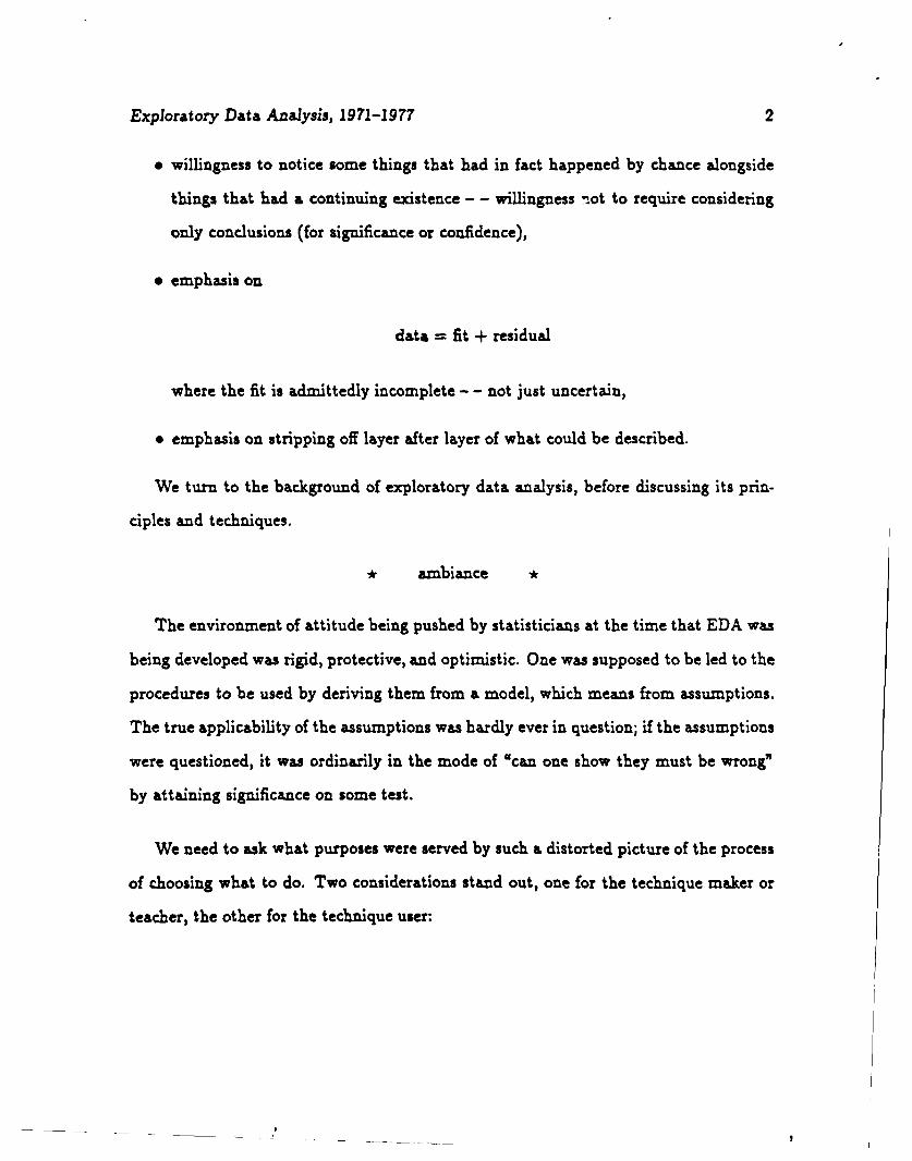
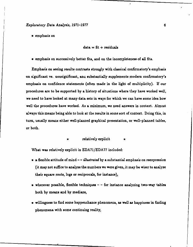
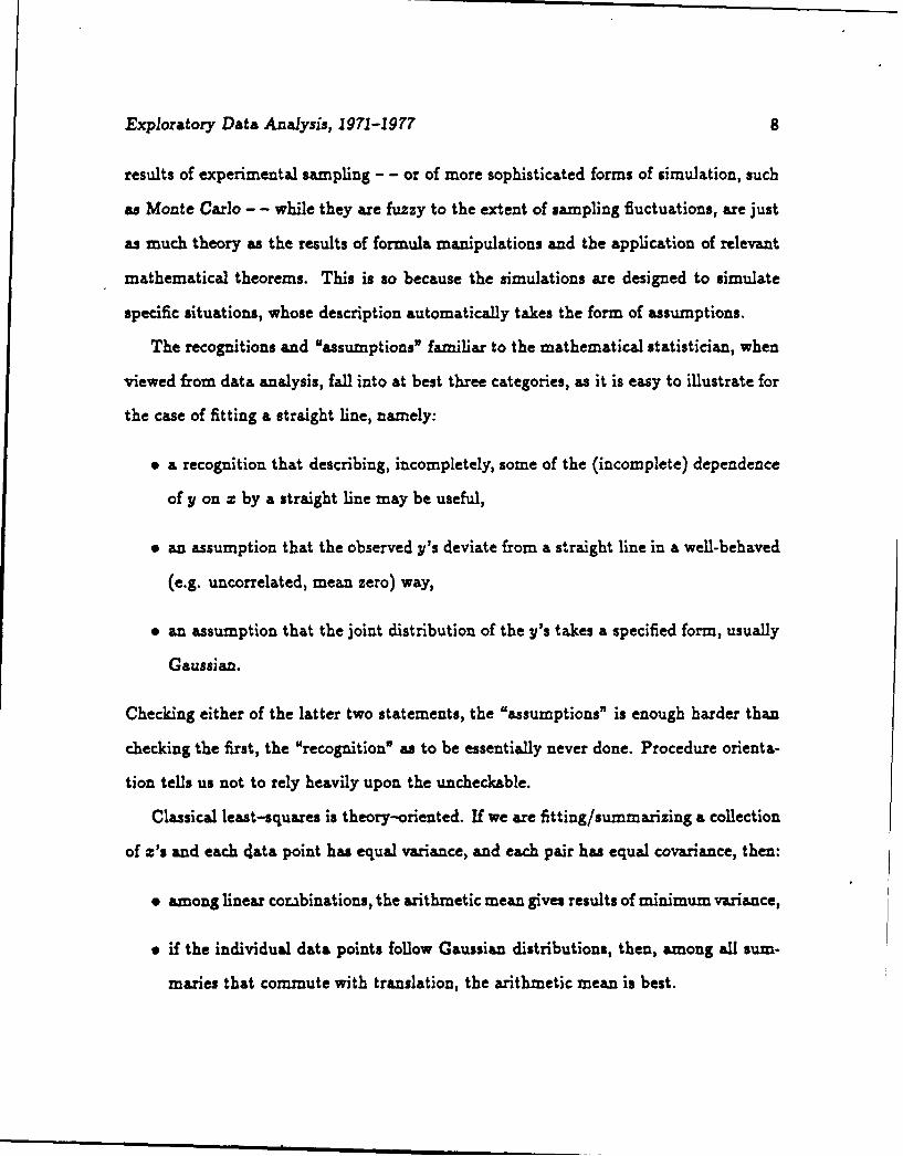
one more constant) to the fit. In the latter case, we can still make a convenient and
revealing picture of the fit, as "exhibits 3 and 4 of Chapter 12" of EDA77 show.

1 5 a
exhibit 10 of chapter 10: East Coast
Plotting basic residuals against comparison values(data from exhibit 9)
E3 kepresemb 8 roincident points
X
•-0 i
-100 0 100
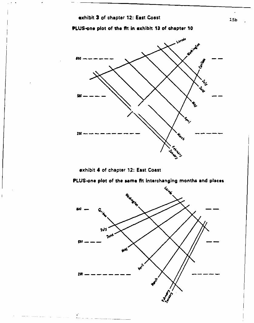
exhibit 3 of chapter 12: East Coast 15b
PLUS-one plot of the fit in exhibit 13 of chapter 10
exhibit 4 of chapter 12: East Coast
PLUS-one plot of the same fit Interchanging months and places
-o

Exploratory Data Analysis, 1971-1977 16
* resistant smoothing *
We turn next to smoothing sequences - - usually sequences in data in time. Our
prime desire is usually not to get better values, but to sort out the slower changes from
the fog induced by both more rapid changes and any errors of measurement or report
that may be involved. If, as is often the case, the errors of measurement or report are
small compared with the rapid changes, the original raw values are a better account of
what actually happened than the smooth. But the smooth may do much more to help
us understand the underlying situation.
Just what resistant (robust) smoothing processes to use depends on our purposes. It
is not at all difficult to identify circumstances where each one of four or more processes
is desirable. Thus it does not seem desirable to go into details here.
But we can illustrate the increase in insight that can be provided. "exhibit 1 of
Chapter 7" shows a dot plot of New York City precipitation for eighty-odd years. A
quick glance sees only a mess; a longer look leads to suspicion of structure, but little if
anything clear. "exhibit 6 of Chapter 7" shows a simple robust smooth of this irregular
data. It clearly suggests recurrence of decade-long periods of either generally higher
or generally lower rainfall. People who had looked at this latter picture might well
have done more to protect New York City from the consequences of the recurrently low
rainfall of the sixties.
When we come to distributions of amounts or counts, we will frequently want to work
with fractions of the data, with counts "below" a chosen value, and with reexpressions
of these fractions. A little care in dealing with such fractions can be important. EDA

exhibit I of chapter 7: 16a
N.Y.C. precipitation
Annual precipitation In Now YorkCity, 1872-1958--actual
Precipitat;en(,wnc he)
It.00
5.) S .
00
00
e
0 0
* S
* 0
g* *
" " 01 l 0
n=

16b
exhibit 6 of chapter 7:N.Y.C. precipitation
Annual precipitation in New York City,1872-1958 -- smoothed
Pre;phatio6(inches~)
eape
40-
M& WO 190 O "
I I'I
I I
* I
0% I II *
t• SI I
IIIII I
II I! I!1t0IO Z I• •

Exploratory Data Analysis, 1971-1977 17
77 urged the use of
is-fraction below
count below PLUS 1/2 count equ:aZ PLUS i/atotal count PLUS 1/3
which is the result of
"* assigning half the cases of = to < and half to >,
"* starting all counts of counts with 1/6.
The need of some start, especially if the fractions are to be re-expressed, is relatively
clear. Exactly which start is not. The choice of 1/6
1/6 = 2/3- 1/2
is compatible with
median of ith orcler statistic
the .3-, point of the cumulative
which is like (i - !)/n for small i.
Three scales for counted fractions, matched at 50% are
f-(1-f)
log. f - log.(' - f)
where f is a started fraction. Their matching is clear in "exhibit 2 of Chapter 15". Of
these three the first is used least - - if we want our analysis to fit in with the data's
behavior - - and the third next-to-least.

exhibit 2 of chapter 15: reference table 17
Pluralities, folded roots, folded logsrkthms--altemative expressions for oountedfractions (take sign of answer from heed of eooumn giving %)
A) MAIN TABLE
+ ILu frooti IfloJ I P frootj I -"
so% use .00 use W/O 85% .70 .76 .87 IS%51 ". .02 - 49 4 .72 .78 .91 1462 .04 48 87 .74 .81 .95 1363 .06 47 88 .76 .84 1.00 1254 .08 46 89 .78 .87 1.05 11
S5% use .10 use 45% 90.0% .80 .89 1.10 10.0%56 -* .12 4- 44 90.S .81 .91 1.13 9.S57 .14 43 11 .82 .92 1.16 95 .16 42 91.S .83 .94 1.19 8.559 .18 41 92 .84 .96 1.22 8
80% use .20 use 40% 12.5% .85 .97 1.26 7.5%61 -- .22 39 93 .86 .99 1.29 7.62 .24 38 93.5 .87 1.01 1.33 6.563 .26 .26 .27 37 94 .88 1.02 1.37 664 .28 .28 .29 36 94.5 .89 1.04 1.42 5.5
I5% .30 .30 .31 3S% 95.0% .90 1.06 1.47 5.0%.6 .32 .32 .33 34 95.3 .91 1.08 1.53 45
67 .34 .35 .35 33 96 .92 1.10 1.59 468 .36 .37 .38 32 96.5 .93 1.12 1.65 3.589 .38 .39 .40 31 97 .94 1.15 1.74 3
70% .40 .41 .42 3W4/o 972% .94 1.16 1.77 28%71 .42 .43 .45 29 97.4 .95 1.17 1.81 2.6"72 .44 .45 .47 28 97.6 .95 1.18 1.85 2.473 .46 .47 .50 27 £7.8 .96 1.19 1.90 2.274 .48 .50 .52 26 U.0 .96 1.20 1.95 2.0
75% .so .52 .55 25% 982% .96 1.21 2.00 1.%
.76 .S2 .54 .58 24 91.4 .97 1.22 2.06 1.677 .64 .56 .60 23 98.6 .97 1.24 2.13 1.478 .56 .59 .63 22 9:.8 .98 1.25 2.21 1279 .58 .61 .66 21 19.0 .98 1.27 2.30 1.0
30% .60 .63 .69 20% 992% .99 1.28 2.41 0.3%11 .62 .66 .72 19 "A, .99 1.30 2.55 0.632 .64 .68 .76 18 3.6 .99 1.32 2.76 0.433 .66 .71 .79 17 "1. 1.00 1.35 3.11 0284 .68 .73 .83 16 100.0% 1.00 1.41 0 0.0
Supplementary Table -

Exploratory Data Analysis, 1971-1977 18
In greater generality, if we see counts, our instinct should be to first reach for some
kind of a square root.
. distributions in bins *
When we want to describe a distribution of values, we can work with fractions -
- preferably as-fractions - - or we can establish a set of "bins" and count how many
values fall in each bin. Our next step, once we have counted in bins, is to take square
roots of these bin counts. "exhibit 5 of Chapter 17" of EDA77 shows a nice example
with bin boundaries (as given in the data source) each at twice the size corresponding
to the previous boundary.
* distribution of counts *
We usually bin samnples of counts, using whatever bin pattern seems to help. It then
usually helps to smooth square roots of these counts. For the number of breeding pairs
of birds (or each species) in Quaker Run Valley, New York it is convenient to work with
logarithms, as in "exhibit 10 of Chapter 17" of EDA77.
. extreme J-shaped distributions .
Use of a logarithmic (e.g. doubling) scale on horizontal axis, with corresponding bin-
widths, will help many distributions that are, to use the time-honored term, reasonably
"J-shapL.d" with a long tail to the right. Some distributions are much too J--shaped,
however, to respond to such a mild cure, and something more extreme is needed.
George Kingsley Zipf formulated his rank-size law as
rank(most frequent = 1) TIMES IS size constant

18a
exhibit 5 of chapter 17: gold assays
The smooth (of root counts)ssay
1w
5 0 0 40 16 11D 040
Gri (pm4Owaity peDta

18b
exhibit 10 of chapter 17: valley birds
The smooth and the rough (of roots of counts of species bynumbers of breeding pairs, from exhibit 9)
7 1 I I FI

Exploratory Data Analysis, 1971-1977 19
As a universal law it is rather worse than most "universal laws". As a place to start, it
is quite useful. If we define "completed rank" by
drank = rank of the last individual of the given size
then we may plan to plot
%/(size = basic count) TIMES (erank)
which Zipf would have constant, against
log(size = basic count)/(c'rank))
the resulting plot seems, often, for very J-shaped data, to be easy to describe. "exhibit
4 of Chapter 18" of EDA77 shows an example from econometrics, where the basic count
is the number of papers at meetings or in the journal of the Econometric Society. Here
721 authors contributed 1 to 46 papers - - and the plot is just a line segment - - but
not a horizontal one.
"exhibit 7 of Chapter 18) of EDA77 shows a similar plot for one year of papers in
atomic and molecular physics where 109 journals included 1 to 372 papers each in this
field. The picture would be simple to describe if it were not for the one journal with 372
papers - - the Journal of Chemical Physics. Leaving that one journal out, thus going to
106 journals with 1 to 79 papers each, as shown in "exhibit 8 of Chapter 18" of EDA77,
produces a plot that is almos as simply describable - - by two segments of straight
lines.
We do not see, in these examples, the horizontal line that Zipf's Law would call for,
even if we do get things that are simply describable. Having such simple descriptions,
we naturally look for explanatory ideas, but these have not yet been found. But to quote
EDA77 at page 613:

exhibit 4 of chapter 18: econometric activity 19a
Plot of root of PRODUCT against Ioo of RATIO(numbers in exhibit 3)
Root of?MDCT
10 Total authors 721.//
0
100
-2 0 +2"

19b
*xb 7 of chapter 18: physics papers
Product-fntio plot for papers in atomic and molecular physics
wheret a *&tld jwalM%•T with threw mwbr of
pgt? ..~be rb"t
to 0• a mju rn a p Il
15-
0
a o
*7 - al o f
- ,p ru m*

19c
exhibit 8 of chapter 18: physics papers
The plot for Atomic and Molecular Physics afterremoval of the Journal of Chemical Physics
166t ofWDULCT
,0
X
0
Na
If
X
10"
j~~W , RAIO2

Exploratory Data Analysis, 1971-1977 20
'"We can compare two such distributions quite effectively, and can detect
many of their idiosyncrasies. We can do this without requiring 'a feeling' or
'an intuitive understanding' of what the coordinates in our plot mean."
3 Selected aphorisms
It seems appropriate to close this review by quoting a few emphasized remarks from
EDA77, namely:
"* (page 1) "Exploratory data analysis is detective work,"
"* (page 1) "We do not guarantee to introduce you to the 'best' tools particularly
since we are not sure there can be unique bests."
"* (page 3) 'Exploratory data analysis can never be the whole story, but nothing else
can serve as the foundation stone."
"* (page 16) " Checking is inevitable ...... Our need is for enough checks but not
too many."
" (page 27) "Summaries can be very useful, but they are not the details."
" (page 43) "(We almost always want to look at numbers. We do not always have
graph paper.) There is no excuse for failing to plot and look (if you have ruled
paper)."
"* (page 52) "There is often no substitute for the detective's microscope - - or for
the enlarging graphs."

Exploratory Data Analyais, 1971-1977 21
"* (page 93) "We now regard reexpression as a tool, something to let us do a better
job of grasping data."
"* (page 97) "Most batches of data fail to tell us exactly how they should be analyzed."
(This does not mean that we shouldn't try.)
"* (page 128) "There cannot be too much emphasis on our need to see behavior."
"* (page 148) "WVhatever the data, we can try to gain by straightening or by flattening.
When we succeed in one or both, we almost always see more clearly what is going
on."
"* (page 157) "1. Graphs are friendly ........ 3. Graphs force us to note the
unexpected; nothing could be more important ....... 5. There is no more reason
to expect one graph to 'tell all' than to expect one number to do the same."
"• (page 586) "Even when we see a very good fit - - something we know has to be
a very good summary of the data - - we dare not believe that we have found a
natural law."
"* (page 695) "In dealing with distributions of the real world, we are very lucky if (a)
we know APPROXIMATELY how values are distributed, (b) this approximation
is itself not too far from being simple."
* close *
So much for EDA71-77, we will take an up-to-date snapshot next time.

Exploratory Data Analysis, 1971-1977 22
References
[1] Hoaglin, D.C., Iglewicz, B. and Tukey, J. W. (1986m). Performance of some resistant
rules for outlier labeling. J. Amer. Statist. Assoc. 81, 991-999.
[21 McGill, R, Tukey, J. W. and Larsen, W. A. (1978a). Variations of box plots. American
Statistician 32, 12-16.
[3] Tukey, J. W. (1971a). Ezploratory Data Analysis. Volume II, limited preliminary
edition. Addison-Wesley, Reading, MA. (Also Volumes I and III.) (Available from
University Microfilm, Inc.)
[41 Tukey, J. W. (1977a). Exploratory Data Analysis. First Edition. Addison-Wesley,
Reading, MA.
NOTE: Letters used with years on John Tukey's publications correspond to
bibliographies in all volumes of his collected papers.

Exploratory Data Analysis, 1991-1994 23
PART BExploratory Data Analysis, 1991-1994
The first question we should address is: What has changed in attacking the problems
that were discussed in the 1977 First Edition?
After we deal with the changes, we go on to illustrate, in the 2-way table prototype,
exploratory analysis of variance, which brings together an exploratory attitude and a
bundle of techniques which ought to have been the basis for classical analysis of variance.
Then we sketch the extension to more-way tables.
Finally, we look briefly at what has happened to the philosophy and strategy that
underlies all forms of exploratory data analysis.
1 What has changed in technique?The most obvious changes in technique are, probably:
"* a broader and deeper look at re-expression, particularly ideas of matching and
hiybridization, and, of starting, now not restricted to counted data,
"* serious consideration of newer medians (such as the lomedian) as well as the clas-
sical median, as simple and effective tools,
"* going back to rootograms, ordinary, hanging and suspended,
"* reordering the book to put two-way tables earlier and display of two-dimensional-
distribution behavior later,
"* recognizing no real need for emphasis on the link-up of some exploratory data
analysis techniques with classical distributions.

Exploratory Data Analysis 1991-1994 24
* re-expression *
No form of exploratory data analysis has ever claimed that values, individual or
summar-• necessarily come in large lumps. If we are doing
data = fit + residuals
for a batch of human weights for example, no one would really want to require either
each fitted value - - or the common term in the fit - - to be a multiple of 25 pounds.
(We might, of course, reasonably think that we could get away with individual weights
in single pounds, with no fractions or ounces.)
The treatment of reexpression in Exploratory Data Analysis (EDA) (1977) empha-
sized integer and half-integer powers of the original expression. If expression in the
power family is just another more-or-less fitted parameter, then it is hard to see an
excuse for enforcing such large (half-integer) steps. We are compelled to ask: Weren't
half-integer steps a hangover from days where reexpression was more shocking, so that
having a restricted set of alternatives might avoid - - or at least reduce - - inflammatory
objections?
Other reasons might include:
"* in 1977, hand calculators dealt with integer and half-integer powers much more
easily than with more general yP,
"* an instinctive response to the feeling, still all too widespread, that reexpression is
always intended to specify something fundamental, rather than just a convenient
approximation to what we would choose to analyze after we had spent lots of time
to study unlimited amounts of parallel data.

Exploratory Data Analysis 1991-1994 25
(No one expects an observed average height of 6 feet, 11 and 3/16 inches to be exactly
right. But many of us have, at least at times, felt that the square root was exactly the
right thing to analyze.)
There is much to be said for beginning with a half-integer or integer power (and
with logs if the "power" is zero). We can each collect useful experience about which of
these discrete, rather widely spaced reexpressions is likely to be a good beginning for a
particular kind of data. But that does not mean that we have to want to stop there.
Living with y"41 or y-.*" is much easier once we introduce the idea of matching
reexpressions.
Which alternative choice of A and B are used in
A + By 41
is just a matter of linear coding, and thus not important, since almost all our procedures
commute with linear coding, in the sense that
linear coding (procedure (something))
procedure (linear coding (same something))
Thus, for instance, working with basketball players heights (a) in inches (and frac-
tions), or (b) in feet (and fractions), or (c) inches (and fractions) minus 72, will give
essentially the same results! (As would working in centimeters or yards!) We are free to
choose A and B as we will - - for any purpose. Often an important purpose is to make
the reexpressed values look a lot like the raw values, which we can do by choosing A and
B to make both value and slope (first derivative) match at some y = M. For matching
yP to y, this leads to
M(1 - p) + MH( )P matched at M
~~~~~ ..... .. ..... . ... . . M
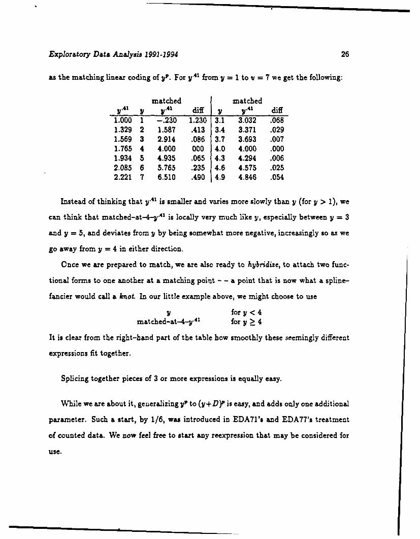
Exploratory Data Analysis 1991-1994 26
as the matching linear coding of yP. For y"41 from y 1 to v = 7 we get the following:
matched matchedY*41 4 V,1 diff y y.41 diff
1.000 1 -. 230 1.230 3.1 3.032 .0681.329 2 1.587 .413 3.4 3.371 .0291.569 3 2.914 .086 3.7 3.693 .0071.765 4 4.000 000 4.0 4.000 .0001.934 5 4.935 .065 4.3 4.294 .0062.085 6 5.765 .235 4.6 4.575 .0252.221 7 6.510 .490 4.9 4.846 .054
Instead of thinking that y-41 is smaller and varies more slowly than y (for y > 1), we
can think that matched-at-4-y .4 1 is locally very much like y, especially between y = 3
and y = 5, and deviates from y by being somewhat more negative, increasingly so as we
go away from y = 4 in either direction.
Once we are prepared to match, we are also ready to hybridize, to attach two func-
tional forms to one another at a matching point - - a point that is now what a spline-
fancier would call a knot. In our little example above, we might choose to use
y for < 4matched-at-4-y-41 for y > 4
It is clear from the right-hand part of the table how smoothly these seemingly different
expressions fit together.
Splicing together pieces of 3 or more expressions is equally easy.
While we are about it, generalizing yP to (y +D)P is easy, and adds only one additional
parameter. Such a start, by 1/6, was introduced in EDA71's and EDA77's treatment
of counted data. We now feel free to start any reexpression that may be considered for
use.

Exploratory Data Analysis 1991-1994 27
I * alternative medians *
While any form of the median is probably nearly the easiest, for hand computation,
of all the desirable summaries for a batch of values, the classical median does require
averaging (of the two central values) whenever there are an even number of values in
the batch. Working with the lomedian - - the ordinary median for an odd number of
values; the lower of the two central values for a batch with an even number of values -
- is just a little easier for hand work - - no average need be found. Moreover:
* it never requires an additional decimal place, because it is always a selection from
previous values (not a calculated function of two or more selected values),
o in simple circumstances, like median polish, it has good convergence properties.
One might think that alternating between
the 3,d highest of SiZ,and
the 3 rYd highest of five,
which are lomedians of a row, and a column, respectively, when lomedian polishing
a 5 x 6 table, has an inherent contradiction, and would not find it easy to converge.
Fortunately it doesn't turn out that way.
We can, however, avoid fractions, always getting integers (which need not all be
selections) by using a barely low median - - or blomedian - - defined for even numbers
of values to be summarized as the mean of the two central values, if this is an integer,
but as 1/2 less than this mean, if this mean is a half integer.
There is some reason to believe that the blomedian:
o leaves fewer zero residuals,

Exploratory Data Analysis 1991-1994 28
* tends to leave a smaller absolute sum of residuals.
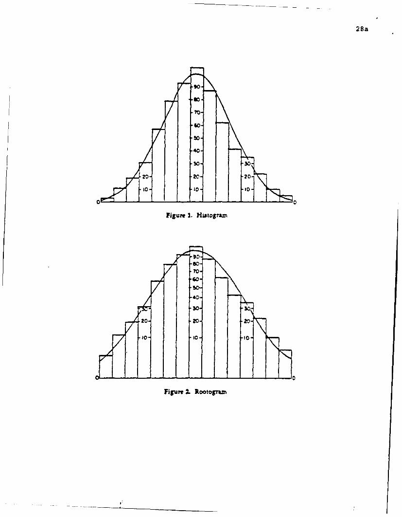
. rootograms .
A histogram is a stack of rectangular columns each of whose heights is proportional to
the corresponding count of values (divided by the width of the column's base, if columns
are not all of the same width.) A rootogram is a stack of columns whose heights are
proportional to the square root of counts/width.
To compare a rootogram with a fitted curve, it helps to slide the columns up or down
to put the center of their upper ends on the curve. The result is a hanging rootogram.
Interpretation is now easier if the picture is now mirror imaged, placing curve and most
of each column below the horizontal axis, thus providing a suspended rootogram. These
are illustrated in figures 1-4. Chapter 17 of EDA (1977) uses the corresponding square-
root scales but omits the names, and columns, focusing on other issues. This appears
to have been unwise.
figures 1-4 about here
* other changes in EDA (1977) *
It is clear that changing the order of the chapters in EDA (1977) would have real
advantages, mainly by bringing the most used techniques to the front. This means
postponing, to later chapters, material like 2-dimensional displays of 2-variable joint
distributions, and, perhaps, omitting material to link some aspects of EDA results to
classical (K. Pearson, W. S. Gosset) distributions.
28a
.'0
.. 0.
70-
40-
so- .30
20- .20 20
0 ~ ~ 1 tog o-
Figure I. Hiutogram~
Figure 2.. Rootograzn

28b
06
Fiur 4 ngspende Rootorram

Exploratory Data Analysis 1991-1994 29
2 Exploratory analysis of variance-- two-way
tables as an initiation
There are important areas, like absorbing the meaning of the results of large plant-
breeding trials for one example, where a satisfactory graphical approach:
"* is badly needed,
"* seems almost certainly feasible,
"* is being worked upon (by Kaye Basford and John Tukey).
We will not try to touch further on this today, but we find it too important to omit
altogether.
A two-way table of response has rows and columns; each row corresponding to a
version of the first factor; each column corresponding to a version of the second factor.
Each response corresponds to a combination of versions, one for each factor. Clearly
we can, and often do, go on to 3, 4, or more factors. The need for some procedures is
clearer when there are more factors, but it still seems worthwhile to begin today with
the 2-factor, rectangular case, covering it in modest detail, and then barely sketch the
extension to more-factor (hyper-rectangular) cases.
* comparison *
We need, first, to confront and compare three approaches to a 2-way table of re-
sponses:
"* the "elementary analysis" of EDA77,
"* the classical analysis of variance,

Exploratory Data Analysis 1 991-1994 30
e synthesis of the two sets of ideas into exploratory analysis of variance,
here "elementary analysis", as we saw in the previous lecture, focuses on decomposing
each observed value as a sum of four pieces:
"* a common term (the same for all values),
"* a row effect (same throughout each row),
"* a column effect (the same throughout each column),
"* a residual (also called a 2-factor interaction).
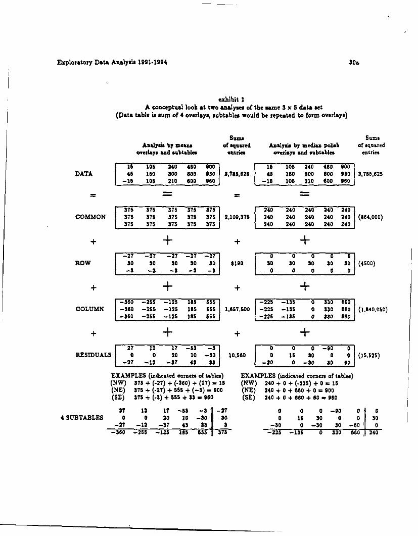
We could regard such a decomposition as putting the corresponding pieces, in the same
pattern as the original data, on one of four overlays. This helps us to think about
generalities, but eliminating the repetitions to reduce overlays to subtables makes it
easier to work with specifics. Exhibit I shows the overlays and subtables for two analyses
of a hypothetical 3 x 5 rectangle of data. One of these analyses extracts means, as in
classical (or, often in exploratory) analysis of variance while the other uses medians,
iteratively, to do median polish (as EDA71 or EDA77).
I exhibit 1 about here
Notice that the two column overlays are not too much alike at first glance. This
happens because the median of the COLUMNS in the analysis to the left is -125 (while
its mean was forced to zero), and mean of the COLUMNS in the analysis to the right
is +126 (while its median was forced to zero). This is mainly compensated for by the
difference of 375-140 = 135 in the COMMON terms, and to a lesser degree by differences
in the other two overlays.
Exploratory Data Analysis 1991-1994 30a
exhibit 1A conceptual look at two analyses of the same 3 x 5 data set
(Data table is sum of 4 overlays, subtables would be repeated to form overlays)
Sums SumsAnaly-si by means of squared Analysis by median polish of squared
overlays and subtables antuies overlays and subtables entries
i 15 105 240 480 9001 15 105 240 460 900DATA 45 1S0 300 600 930 3,785,625 45 150 300 600 930 3,765,625
-15 105 210 600 960 -15 105 210 600 960
375 375 375 375 375 240 240 240 240 240COMMON 375 375 375 375375 2,109,377 240 240 240 240 240 (864,000)
375 375 375 375 3T5 240 240 240 240 240
+ + + +
i-27 -2T 2T-27 -27--fl0 00 001ROW 30 30 30 30 30 $190 30 30 30 30 30 (4500)
-3 -- 3 -3 -3 -3 0 0 0 0 0
+ + + +-360 -255 -125 185 $555 -225 -135 0 330 660
COLUMN -360 -255 -125 165 555 1,657,500 -225 -135 0 330 660 (1,640,050)-360 -255 -125 185 55 -225 -135 0 330 660
+ + + +
27 12 27 -53 -3 I 0 0 0 -90 0RESIDUALS 0 0 20 10 -30 10,560 0 1s 30 0 0 (15,525)
-2T -12 -37 43 33 1-30 0 -30 30 60
EXAMPLES (indicated corners of tables) EXAMPLES (indicated corners of tables)(NW) 375 + (-27) + (-360) + (27) = 15 (NW) 240 + 0 + (-225) + 0 - 15(NE) 375 + (-27) + 555 + (-3) = 900 (NE) 240 + 0 + 660 + 0 = 900(SE) 375 + (43) + 55 + 33 = 960 (SE) 240+0+860+60=960
27 12 17 -53 -3 -27 0 0 0 -90 0 04SUBTABLES 0 0 20 10 -30s 3 0 15 30 0 0 30
-27 -12 -37 43 23 3 -30 0 -30 30 -60 0-360 -255 -125 185 555 375 -225 -135 0 330 660 240
Exploratory Data Analysis 1991-1994 31
Facing up to multiple analyses of the same data can be painful, especially since it
may make it hard to say: "the data show that [some detailed result]." But we need to
remember that this difficulty is in the interests of realism, and should often be accepted.
Of our three approaches, the classical analysis of variance would have gone down
the left-hand column and focused on a table of sums of squares, degrees of freedom,
and mean squares, traditionally (and unhappily) often called the analysis of variance
table (we will illustrate it for these examples shortly, see panel K of exhibit 4). Then it
would have focused on F-tests based on ratio of mean squares and used their results to
determine significance statements.
Elementary analysis would have gone down the right-hand path to the 4 subtables,
and then tried to help us understand them by graphing first the fitted values, in a way
that make row and column effects clear, and does what is usually well enough for the
common, and then display the (large) residuals located according to the plot of fitted
values.
Exploratory analysis of variance is glad to have got us far as the four subtables,
but wishes to press on further, focusing on how one should use the results to answer
questions, as we will now explain.
Exhibit 2 carries on both analyses, continuing with row values - - made from row
effects by adding back the common term. In our example, the difference in common
first noted has to be reflected in a corresponding (approximately the same) difference in
ROW VALUES. The COLUMN values are much more similar in the two analyses, as
they must be, since all the ROW effects are small as are the interactions, so that neither
could compensate for any great difference in COLUMN VALUES. (The central columns
in panel D remind us of the original values that correspond to each ROW VALUE.
Exploratory Data Analysis 1991-1994 32
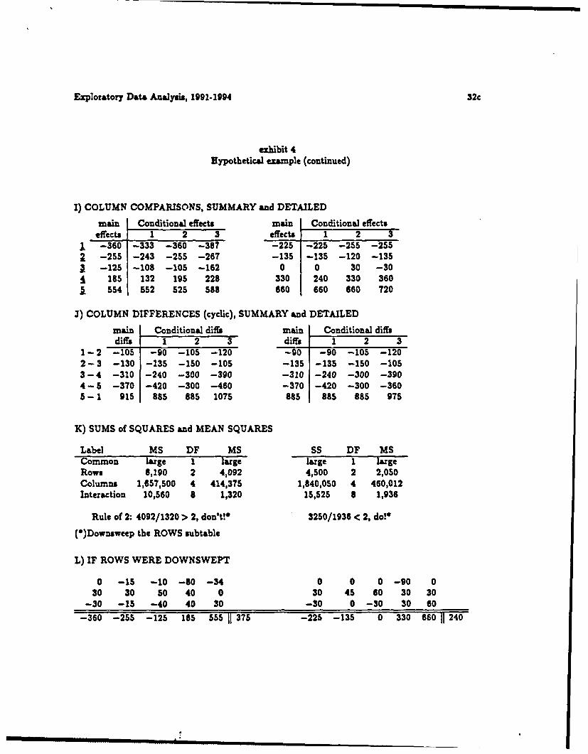
1 exhibit 2 about here
Exhibit 3 begins with the ROW DIFFERENCES, which are only similar in the two
analyses by being small, and the COLUMN DIFFERENCES, which are more nearly the
same in the two analyses. Panel G, the next panel, compares ROW EFFECTS (sum-
marized for all columns) with row effects in individual columns - - CONDITIONAL
ROW EFFECTS. (In a simple two-way example, these conditional row effects reflect
individual observations in the original table.) Panel H, does the same for ROW DIF-
FERENCES. In either case, the conditional results are not at all identical, but do NOT
differ from the summary results enough as to make the summary results always nearly
useless as a single replacement for all the conditional results.
I exhibitb 3 and 4 about here
Panels I and J, in exhibit 4, show similar behavior for COLUMN EFFECTS COM-
PARED and COLUMN DIFFERENCES. The next Panel - - Panel K - - reports sums
of squares (calculated in exhibit 1) and mean squares, found from
Mean Square -Sum of Squares
Degrees of Freedom
for both analyses. The last line compares, with 2.00, the ratio of mean square for rows
to mean square for interaction. For the left-hand analysis, this ratio is larger than 2, so
we are instructed to leave the ROW subtable in place, as possibly useful. (We may want
to ask for a conditional answer, but a summary one may serve.) For the right-hand
analysis, the ratio is less than 2 so we are instructed to get rid of the ROW subtable
(since the (unconditional) ROW EFFECTS are unlikely to be useful) by downsweeping
it into the interaction subtable.

Exploratory Data Analysis, 1991-1994 32a
exhibit 2Hypothetical example of two-way analysis
A) DATA (hypothetical)
15 105 240 480 90045 150 300 600 930
-15 105 210 600 960
B) TWO ANALYSES
27 12 17 -53 -. 3 -27 0 0 0 -90 0 00 0 20 10 -30 30 0 15 30 0 0 30
-27 -12 -37 43 33 -3 -30 0 -30 30 60 0-360 -255 -125 185 555 375 -225 -135 0 330 C60
27 + (-17) + (-360) + 375 = 15 0 + 0 + (-225) + (240) = 15examples: 20 + (30) + (-125) + 375 = 300 30 + (30) + (3) + (240) = 300
33 + (-3) + (555) + (375) = 960 10 + (0) + (660) + (240) = 960
C) ROW (fitted) VALUES
-27 + (375) = 348 0 + (240) = 24030 + (375) = 405 30 + (240) = 270-3 + (375) = 372 0 + (240) = 240
D) COLUMN (fitted) VALUES To replace
-380+(375) = 15 -15,0,45 -255+(240) = 15-255+ (375) = 120 105,105,120 -135+ (240) = 155-125+(375) = 250 210,240,300 0+(240) = 240
155 +(375) = 530 480,600,600 330 +(240) = 570555 + (375) = 930 900,930,960 660 + (240) = 907

Exploratory Data Analysis, 1991-1994 32b
exhibit 3Hypothetical example (continued)
E) SUMMARY ROW DIFFERENCES
Rows RowsColumns 2 3 Columns 2 3
1 57 24 1 30 02 x -33 2 -30
x
F) SUMMARY COLUMN DIFFERENCES
2 3 4 5 2 3 4 51 105 235 515 915 90 225 555 8852 x 130 410 8102 x 235 465 7553 x 280 680 x 330 660
x 400 x 330
G) ROW EFFECTS COMPARED, SUMMARY and DETAILED
main Conditional effects main Conditional effectseffects 1 2 3 4 5 effects 1 2 3 4 5
1 --27 0 -15 -10 -60 -30 0 0 0 0 -30 030 30 30 50 40 0 30 30 15 30 0 30
S-3 -- 30 -15 -40 40 30 0 -30 0 -30 30 60
B) ROW DIFFERENCES, SUMMARY and DETAILED
main conditional diffm main conditional diffsdiff. 1 2 3 4 5 diffs 1 2 3 4 5
1-2 -57 -30 -45 -60 -100 -30 1-2 -30 -30 -15 -30 -30 -302-3 33 60 45 90 0 -30 2-3 30 60 15 60 -30 -303-1 24 -30 0 -30 100 -60 3-1 0 -30 0 -30 -60 60
Exploratory Data Analysis, 1991-1994 32c
exhibit 4Eypothetical example (continued)
I) COLUMN COMPARISONS, SUMMARY and DETAILED
main Conditional effects main Conditional effectseffects 1 2 3 effects 1 2 3
1 --360 -333 -360 -387 -225 -225 -255 -255--255 -243 -255 -267 -135 -135 -120 -135
1 --125 -108 -105 -162 0 0 30 -30185 132 195 228 330 240 330 360
5 554 552 525 588 660 660 660 720
3) COLUMN DIFFERENCES (cyclic), SUMMARY and DETAILED
main Conditional difis main Conditional diffsdiffs 1 2 3 diffs 1 2 3
1 -2 -105 -90 -105 -120 -g0 -90 -105 -1202-3 -130 -135 -150 -105 -135 -135 -150 -1053-4 -310 -240 -300 -390 -310 -240 -300 -390
4 - 5 -370 -420 -300 -460 -370 -420 -300 -3605-1 915 885 885 1075 885 885 885 975
K) SUMS of SQUARES and MEAN SQUARES
Label MS DF MS SS DF MSCommon large 1 large large 1 large
Rows 8,190 2 4,092 4,500 2 2,050Columns 1,657,500 4 414,375 1,840,050 4 460,012Interaction 10,560 8 1,320 15,525 8 1,936
Rule of 2: 4092/1320 > 2, don't!* 3250/1936 < 2, do!*
(O)Downsweep the ROWS subtable
L) IF ROWS WERE DOWNSWEPT
0 -15 -10 -80 -34 0 0 0 -90 030 30 50 40 0 30 45 60 30 30
-30 -15 -40 40 30 -30 0 -30 30 60-360 -255 -125 185 555 1 375 -225 -135 0 330 660 II 240
Exploratory Data Analysis 139, 2 .9 4 33
Panel L shows the consequences of downsweeping "ROWS" in both analyses, to the
left where we are told not to do this and to the right where we were told to do this. If we
come out with either instance of this pattern of subtables, we would be telling ourselves
not to answer any questions about rows unconditionally. If we had left our subtables
as in Panel B (exhibit 2), we would be telling ourselves that we have a choice between
answering questions about rows, either unconditionally for any column like one in the
data that may be coming to us - - maybe even more generally - - or conditionally (with
specific application to one of the columns represented in the data). This is our choice, a
classical choice between greater variability (when conditional), and greater bias (when
unconditional) - - between using less, but more relevant, data and using more, but less
relevant, data. This is an example of a very widespread problem.
3 Exploratory analysis of variance, the general
factorial case
In a 3-or-more-way example, we follow the same sequence of steps as for a two-way
table:
"* upsweep by means,
"* calculate mean squares,
"* downsweep, wherever the appropriate ratios of mean squares are < 2.
The resulting decomposition can be pictured by the remaining subtables and their sizes
can be described, often quite inadequately, by the remaining (pooled) mean squares.
It will continue to be important to remember that most of the questions we want to
"ask are questions about differences, so that we will usually ask: either about main effects

Exploratory Data Analysis 1991-1994 34
or differences of main effects which will equal differences of main values (but not about
main values themselves), or about interactions (which are at least double differences).
It will still be important to know to how conditional a question we seek an answer, and
to consider how conditional an answer it will pay us to use in reply.
* important aspects touched upon *
Exploratory analysis of variance emphasizes flexibility and practical guidance. This is
illustrated by the process of (i) sweep everything up, (ii) selectively sweep some subtables
back down, and (iii) guide selection by indicated usefulness, not a P-value.
Exploratory analysis of variance has a place for robustness, especially if designed to
feed into the conventional analysis. Exotic values, if any, are identified in comparison
with the other entries in the same subtable, and, from then on, are treated as "missing"
in a conventional analysis of means.
Exploratory analysis of variance is not bothered by doing both unrobust and robust
analysis on the same data - - and turning neither one away.
Multipic-comparisons and conclusions (significance or confidence statements), ap-
pear in exploratory analysis of variance because intuition is no longer an adequate guide
to what ought to be noticed. (They are rarely needed in the simpler procedures and
results of EDA (1971 or 191'7).)
More flexible (and diverse) expressions enter easily.
* literature and work in progress
One book in print (Hoaglin, Mosteller, Tukey 1991).
One book in preparation (Hoaglin, Mosteller, Tukey 199?).
Exploratory Data Analysis 1991-1994 35
One long paper at the printer (Tukey 1993.)
Work in progress on the graphical description of (hyper)rectangular blocks of data
as illustrated by large plant breeding trials.
. conclusions *
Classical analysis of variance pretended to be exclusively engaged in drawing conclu-
sions. Some of us with wide experience in using classical analysis of variance have felt,
for some time, that 90% of the uses of classical analysis of variance were exploratory,
no matter what the books and professors pretend. But arguing for 99% - - or higher -
- would be a mistake. Some uses of classical analysis of variance do naturally involve
conclusions. So we do need to ask what we should do to be effective with our conclusions.
Classical analysis of variance yammers about "F-tests" based on ratios of mean
squares, that are dirtted toward the question "have we shown at least some differences
among - -" whose answer is almost worthless.
We ought to focus on bouquets of observed differences, asking either:
"* for which of them are we to believe that the underlying direction is the same as
the observed direction? (Which significance-type conclusions?),
"* within what intervals, centered at the observed differences, are we to believe that
the underlying difference falls? (What confidence-type conclusions?)
We can handle either of these in terms of the product of two numbers: (i) a value to be
found in a studentized range table, and (ii) the square-root of an error term (often a lower
level mean s:uare; sometimes a linear combination of such mean squares). The result is
a multiple-comparison procedure, specifically a multiple-difference procedure. We can
Exploratory Data Analysis 1991-1994 36
most nearly match the e.ror-rates associated with the classical analysis of variance by
looking at the 5% point of the studentized range (for k candidates and v degrees of
freedom in the error term), thus "controlling" the probability of at least one error in our
confidence statements.
To view the answer, provided that the variability that ought to be associated with
differences between different pairs of values does not vary too much, we do well to
represent our understanding of our uncertainty by a set of "notches". The basic idea is
explained in exhibit 5, which shows, first a case where the notches overlap, so that the
direction of the difference is uncertain, but second, an example where the notches do not
overlap, so the direction of A - C is certain, but the amount is only settled to limited
accuracy. Exhibit 6 shows a larger example - - for a factor with 13 versions.
exhibit 5 and 6 about here
* some of the novelties *
Some of the novel approaches (or techniques) in exploratory analysis of variance are
listed in exhibits 7 to 11.
* hints *
If we feel exploratory, but make some use of conclusions, it would be a mistake to treat
all negative conclusions - - non-significances or confidence intervals that cover zero - -
alike. A basic part of exploratory is to plan to make remarks about some happenchances
as well as about some real effects. This means that small enough differences should be
forgotten about, while larger differences, for example that almost reach significance,
need to be mentioned. What guidance should we give the user? It should be:

E-xploratory Data Analysis, 1991-1994 36a
exhibit 5The basic rationale of notches
A Acould be BI
anywhere could be
here anywhere
here nine possibleA-B diffs
A (arrows from a possible B to a possible A)X ~ could beanywhere
here Ccould be
anywhere (XLA
herenine possible
A-C diffs
(arrows from a possible C to a possible A)
NOTE: Notches are only to be used in pairs to teachus about differences. If we only ask about intervals forthe separate values, with no attention to differences weget somewhat longer "notches" based upon the Stu-dentized maximum modulus rather than on the Stu-dentized range.

Exploratory Data Analysis, 1991-1994 36b
exhibit 6An example of a notch display for 13 versions
S
, "
l a

Exploratory Data Analysis 1991-1994 37
exhibit 7Novel aspects of exploratory analysis of variance, 1
First in terms of what to expect:
"* omnibus answers - - like "some of these are different" - - are nearlyworthless,
"* (global) main effects are unlikely to be useful unless they overridedifferences among the corresponding conditional effects stronglyenough,
"* conditional main effects (or conditional interactions) frequently pro-vide the answer of choice,
"" tables of mean squares and statements of significance/non-significanceare inadequate and need to be replaced,
"* the best replacement is probably tables of numerical results thatapply as generally as is reasonable given the data, combined withtables of the numerical adjustments that would need to be appliedin each instance of conditioning further.

Exploratory Data Analysis 1991-1994 38
exhibit 8
Novel aspects of exploratory analysis of variance, 2
Next we turn more to how to behave. Here we need to:
* think in terms of overlays; work in terms of subtables - - (tables
full of (approximate) numbers, not just symbols with subscripts,
* start by upsweeping all that we can; then downsweep as guided by
the rule of 2,
"* use downsweeping - - or its consequences - - to tell us what ques-
tions not to ask - - to tell us when it is reasonably clear that we
need to be more conditional,
"* be prepared to be more conditional than this minimum, when ap-
propriate,
"* be prepared to use hybrid reexpression - - and be pretty flexible
about reexpression.

Exploratory Data Analysis 1991-1994 39
exhibit 9Novel aspects of exploratory analysis , 3
Next some somewhat more sophisticated points. Here we need to:
"* think about using stability of variance as moderately important forthe choice of reexpression,
* introduce robustness in a "cookie-cutter" mode classifying eachvalue as "usual" or "exotic",
"* recognize that
*. choice of error terms involves more detail, and can contributemore to realism than we have thought.
a* that, when we want to lean toward conclusions, displays of"notches" seem the effective way to do this.
ee some notches do not do badly in dealing with hints,
.e the order in which we apply various procedures and subproce-dures deserves more careful thought.
I

Exploratory Data Analysis 1991-1994 40
exhibit 10Novel aspects of exploratory analysis of variance, 4
When it comes to doing a more thorough analysis, we need to:
* pay more attention to choosing an expression for which thevariance is more nearly constant,
* when describing interactions, look harder at details, perhaps
through values of bicomparisons,
e look for version-related differences in variability (not easy).
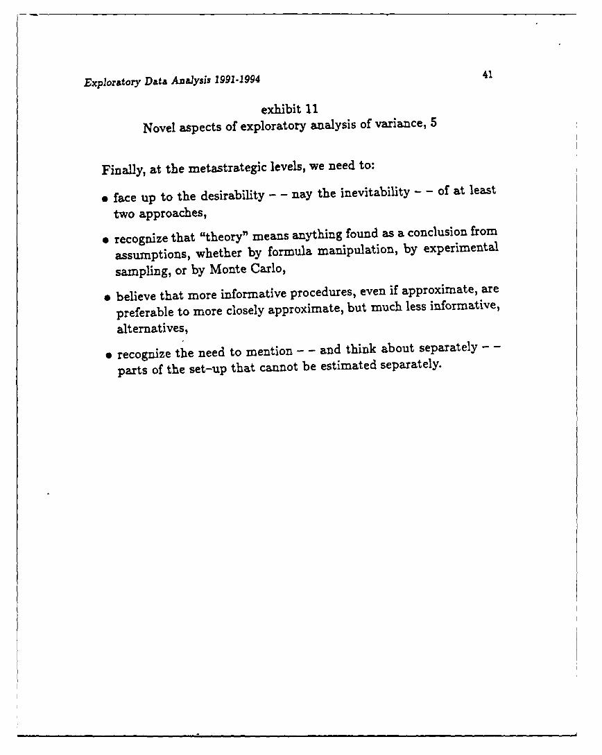
Exploratory Data Analysis 1991-1994 41
exhibit 11
Novel aspects of exploratory analysis of variance, 5
Finally, at the metastrategic levels, we need to:
"* face up to the desirability - - nay the inevitability - - of at least
two approaches,
"* recognize that "theory" means anything found as a conclusion from
assumptions, whether by formula manipulation, by experimental
sampling, or by Monte Carlo,
"* believe that more informative procedures, even if approximate, are
preferable to more closely approximate, but much less informative,
alternatives,
"* recognize the need to mention - - and think about separately - -
parts of the set-up that cannot be estimated separately.

Exploratory Data Analysis 1991-1994 42
"* relatively simple,
"* moderately flexible,
to allow for the fact that just what deserves mention is conditioned by other information
and insights beyond what is in the data - - we need guidezones, not guidelines.
We are here beginning to establish a new process, with new (and this time, deliber-
ately quite rubbery) standards. As always, these conditions mean that we have to begin
as best we can, and watch what the more experienced users tend to do. After that, we
may need to revise our zones. At this point we can offer only an initial version of hint
guidezones, which we do in exhibit 12.
exhibit 12 about here
Clearly we shall have to be careful about how we label and use hints.
Graphically, we can use the same notches as before, adding a horizontal stripe above
and below the waist, extending from 1/5 to 1/3 of the way from waist to end. The
boundaries between hint zones now correspond to:
"* between conclusion and Zone A: One end of each notch matching the other end of
the other notch,
"* between Zones A and B: end of one notch at outer edge of near stripe of the other
notch,
"* between Zones B and C: end of each notch at waist of the other notch,
"* between Zone C and "no comment": end of one notch extends beyond waist of the
other, but only as far as the beginning of the stripe.

Exploratory Data Analysis, 1991-1994 42a
exhibit 12A set of guidezones for gaiding mention of differences in terms of what fraction ofthe difference that is barely worth a conclusion (just reaches 5% significance, has
95% confidence interval touching zero)
Zone (observed difference)(barely conclusive difference) Recommended action
Zone A 2/3 < ratio < 1 most occurrences arecandidates for mention'
Zone B 1/2 5 ratio 5 2/3 reasonable chance of beinga candidate for mention*
Zone C 2/5 :5 ratio _5 1/2 exceptionally interesting casesmay be candidates for mention'
"Mention often needs to be restricted to a specified number of differences,perhaps 8. Selecting these, when we would otherwise have mentioned moreshould depend - - as did our recognition of them as prime candidates - -on both the observed ratio and other considerations.

Exploratory Data Analysis 1991-1994 43
Exhibits 13, 14, and 15 show the boundaries of the three zones.
I exhibits 13, 14, 15 about here
For one who must oversimplify - - destroying the flexibility of 3 hint zones - - the
original notches serve (without stripes) to separate the union of zones A and B from all
else by the relation of the end of one notch to the waist of the other.
4 Generalities
What general phenomena in the development of exploratory data analysis should be
recognized? Probably these, which tend to summarize what we have said above:
"* Procedure orientation has become somewhat more explicit.
"* A few alternatives are being taken seriously (e.g. robust and non-robust analyses).
"* Attempts to provide all necessary support of intuition, especially in complicated
situations - - using apparently confirmatory procedures to do this without shame.
"* Moderate flexibility of expression.
"* Almost all strategy a judgment matter.
"* Much guidance for tactics.
"* Multiple-comparison procedures and notch plots, for conclusions and, perhaps, for
hints.

Exploratory Data Analysis, 1991-1994 43a
exhibit 13
Extremes of hint Zone A - - mention likely - - unless list too long
everfap 1/3 overlap = 0
intermediatesitut•tions
awe inZone A
* .6 • *
8 d.4* - b

Exploratory Data Analysis, 1991-1994 43b
exhibit 14
Extremes of hint Zone B - - mention reasonable - - unless list too long
Overlap 1/2 overlap = 1/3
intermediatesituations
are inZone B
C'" C iC.
.• C C C
*_s~ *.* .C *C

Exploratory Data Analysis, 1991-1994 43c
exhibit 15
Extremes of hint Zone C - - mention unlikely, but possible
orlap 3/5 overlap 1/2
intermediate
.0• situations
are in , @
Zone C
0**E *aA

Exploratory Data Analysis 2991-1994 44
References
11] Hoaglin, D.C., Mosteller, F., Tukey, J.W. (1991h). Fl'ndamentals of Exploratory
Analysis of Variance. Wiley, New York, 430 pages.
12] Hoaglin, D.C., Mosteller, F., Tukey, J.(199?).
13] Tukey, 3. W. (1971a etc.). Exploratory Data Analysis. Volumes 1, 11, and III Lim-
ited Preliminary edition. Addison-Wesley, Reading, MA. (Available from University
M.icrofilms, Inc.)
14) Tukey, 3. W. (1977a). Exploratory Data Analysis. First Edition. Addison-Wesley,
Reading, MA.
15] Tukey, J. W. (1993?). Exploratory analysis of variance as providing examples of
strategic choices. Proceedings Data Analysis and Robustness (S. Morgenthaler ed.).
NOTE: Letters used with years on John Tukey's publications correspond to
bibliographies in all volumes of his collected papers.
Exploratory Data Analysis, 1995-2005 45
PART CExploratory Data Analysis, 1995-2005
Any presentation with such a title can only be a set of dreams and targets. But
it may usefully point out likely avenues of advance, so long as it is not thought of as
pretending - - or as likely to prove - - to be exhaustive. As parts of it are done, and
related topics are worked on, emphasis - - and probably content - - will need to change.
Like the previous lecture, this third lecture will be divided into a major topic, here
regression, and a collection of generalities.
1 RegressionThree decades or so ago, I heard W. G. Cochran sagely pronounce regression as "the
worst-taught part of statistics". While there has been some, perhaps even considerable,
improvement, this characterization is still appropriate.
Yet together, analysis of variance and regression provide a very large share of all the
statistically-structured analysis of data. And much of what is left over involves analogies
to one or both of these areas.
In regression, the consequences of procedure orientation differ from those of theory
orientation even more than elsewhere. Much regression analysis is carried out out on
weak data: either on data not collected for the purpose, or on variables where much
more relevant variables would have been collected, were this possible. The idea that
the data must certainly, if properly massaged, be able to answer the burning question is
most seductive and dangerous in such circumstances.

Exploratory Data Analysis, 1995-2005 46
. exploratory regression: description or prediction?.
We can offer a reasonable scale of kinds of response to a plot of y vs z, namely:
* it's reasonably straight,
e it's rising (as z rises),
* a fitted line has a slope of roughly so-and-so much,
* we can predict, from this slope, the effect on y of changing z a specified amount.
We can be moderately procedure-oriented at each of the first three steps - - although
we may have to admit that what we see is a consequence of how the data was distorted
by the collection process, as well as a consequence of how the world operates. But we
cannot go nearly as far with the fourth step.
In general, description may be quite valuable - - in another way - - by offering
residuals that represent what is so far undescribed - - once we have our hands on them,
we may be able to describe some of the structure of what remains!
The striking example that Charlie Winsor used to use to good effect in Ames, Iowa
was y = illegitimate birth rate by state and z = % membership in Protestant evangelical
churches (also by state) where, for the last Census that collected :, the relationship of
V to : was quite strong, with y larger where z was larger. 'Yet no one would - or should
- believe that increasing z would increase y.
Any adequate account of regression, exploratory or confirmatory, has to give heavy
emphasis to the distinction between desciiption and the probable consequences of change.
Clearly what goes on in almost all such instances is that there are other variables
which are involved in the real world, but not present in our regression. (Some of those
Exploratory Data Analysis, 1995-2005 47
that are included may make trouble, also.) The world is full of surrogates, and their
impacts on what seem to be relationships can be large indeed.
This problem is worth a second example: Gross's study of school principals, where
he collected opinions of both those the principals supervised, and those who supervised
the principals. Since these two views agreed as to who were better principals, and who
were worse, we should probably regard this y as quite well measured. If z is number of
graduate courses taken in education, then V and z are visibly related - - the more courses
taken the poorer performance as a principal. If z is number of graduate courses taken
in educational administration, the relation is in the same direction, but stronger. Does
anyone believe that having a particular individual avoid graduate courses in education
would make that individual a better principal? I doubt it. I know I do not. (But giving
graduate courses less weight in choosing among candidates for promotion to principal
might be an effective response.)
The fact that information about prediction may be badly needed is often not adequate
reason for the available data to support inferences about prediction.
We need to be very clear about the description-prediction antithesis, both when
working with a single x and when working with several z's.
In particular, when we fit
a + b2XI + b2=2 +-. + bk~k
with correlated z's (for convenience, all of the same variability) there is no reason to be
sure that the z with the largest fitted b, is the most important of the z's. The same is
true for the :i with the largest t-statistic.

Exploratory Data Analysis, 1995-2005 48
2 Enhanced techniques for exploratory regression
As matters of technique, rather than matters of broad principle, there are areas we
can point out where exploratory regression should be strengthened, and probably can
be. These include:
"* diagnosing needs for changes in expression,
"* providing greater fexibility of expression,
"* investigating exploratory path regression,
"* robust fitting, alone and in combination,
"* emphasizing multiple answers,
* graphical techniques for simultaneously examining two or more alternative fits,
* looking harder at "stopping rules" - - rules needed whenever one aspect of explo-
ration, as it probably ought usually be, is how many x's to put into a reasonable
description - - not too few, and not too many!
Let us say a little more about each of these.
* diagnosing for re--expression
There are tools already in use for asking whether the data suggests changing how yi
is expressed, or how some of the z, are expressed, or both. In a two-way table - - the
simplest serious pattern of data - - we have used, in exploratory data analysis and in
exploratory analysis of variance, the diagnostic plot, and its extensious, to learn about
re-expressing our response. We can, and should, carry this sort of procedure over to

Exploratory Data Analysis, 1995-2005 49
many regression situations, and parallel it, if not combine it, with the techniques already
available for regression.
* clarifying how we think about re-expressions
As we make use of flexibility of forms of expression in exploratory analysis of variance
- - and elsewhere - - particularly by effective use of matching re-expression, we will have
flexibility useful in exploratory regression as well. Looking at "z2 instead of x, when, for
example, 900 _ x <:< 1100 as a great big change - - Why the new regression coefficient is
only a thousandth the size of the old one! - - is allowing us to mislead ourselves without
reason or excuse.
Using 22 instead of 500 + x2/2000 saves space: in a book, on a blackboard, or on
a piece of paper. But, if we are doing linear regression, using one or the other gives
ezxctly the same fitted values and the same residuals. Over the range from 900 to 1100,
we have the following correspondences:
500+ : 2
905 900 810,OO951.2 950 902,5001000 1000 1,000,000
1051.2 1050 1,102,5001105 1100 1,210,000
Clearly the first column is an only slightly bent version of the second, while the third
column seems "Oh, so different from the other two".
Telling someone that x 2 will do better than x is really saying, over such a relatively
narrow range, that a small bend in the x-values may help. It is not saying that something
like changing 1,000 into 1,000,000 needs to be done.

Exploratory Data Analysis, 1995-2005 50
* exploratory path regression *
Path regression, where we impose limitations on several regressions as a way of ex-
pressing our insights about mechanisms, deserves combination with exploratory, procedure-
oriented ideas and techniques. In the principalship situation, for example, we might
diagram the relationship of key variables as follows:
inherent ability ( felt need for (graduate\of candidate graduate courses to .-.. , courses
support promotion taken
performanceif promoted
We can't do path regression here because we have no measures of inherent ability or
of felt need, but just drawing the arrows offers a plausible explanation for the observed
relationship of the two right-hand variables.
There will be many data sets where we can try path regression seriously, often com-
paring the results of using two or more path patterns.
* robust regression *
Even if robust regression, which need not be very complicated to be useful, were
to only attract our attention to - - and urge on our inquiry about - - the apparently
exotic data points, it would usually be worth the effort. There are few data sets, indeed,
that do not deserve the basic troika: one non-robust fit, one robust fit, and one careful
examination of the differences. Notice that the careful comparison will usually be needed
to understand the data in the light of bcth analyses, and not just to support hubris by
trying to decide which one is "right".
Exploratory Data Analysis, 1995-2005 51
* non-data-directed and triskeletally fitted composites *
If we are realistic, the proper reaction to a collection of substantially highly correlated
='s is not to try to find the important z - - both because the data is not likely to allow
you to find such an z if, indeed, one such exists, and because the existence of one such z
is rather/quite unlikely. Instead, the better strategy is to concoct a composite (or two,
or conceivably three) whose coefficients are n~ot supposed to reflect relative importance
of influence on y, and then fit one (or perhaps two or three) coefficients multiplying
the composite (or composites). One great gain from doing this is avoiding conning the
reader into the foolish idea that anyone knows, or can learn from available data, which
of the z's are important.
Indeed, it is not unlikely that our composite, even if its coefficients were picked using
a small (or large) crystal ball, is more effective, more important than any single x. When
this is so, and especially when the effective amount of data at hand, allowing for the
high correlation among the z's (inevitably reflected in less information per point!), is
small enough to make fitting more than one constant wasteful, there are extra dividends
by using the composite.
Sometimes we can clabber together our composite solely out of general knowledge -
- making a composite that is not data driven. At another extreme, we can use the data
in a deliberately incomplete way as when we use only the univariate relationships of y'
to each of the z's alone as a basis for composite formulation - - eschewing, wisely, a
multivariate approach. This might naturally be called triskeletal selection, since it uses
only I row, I column, and I diagonal of the (k + 1)-by-(k + 1) symmetric matrix of
variances and covariances of V, zi, X2 ,.-., zk . With conventional amounts of data,
triskeletal selection of a composite (when possible, based upon comparisons uncorrelated

Exploratory Data Analysis, 1995-2005 52
with those that are our real concern), followed by fitting one constant, can easily out-
perform multivariate simultaneous fitting of the bi corresponding to a cluster of highly
correlated zi.
Here, as so often elsewhere, it takes more data to adequately support formal opti-
mization than we usually have - or dream about. Trying to use inadequately supported
formal optimization wastes information and increases variability (of fit, coefficient, or
residuals) unnecessarily.
* exploring multiple answers *
We have pointed earlier to keeping multiple answers. It could be argued that the
style of physical science is to go for the right answers. This is plausible for chemistriy
and cla.ssical physics, but for many decades the particle-wave duality has made most of
modern physics live with incompatible pairs of answers. For those with a mathematical
or tightly formal-logical bent this is bad enough, but is only the beginning.
The only paper deliberately reprinted in the same journal - - Science - - after 70
-years is a paper by the great geologist, Thomas Chrowder Chamberlin, one of whose main
points was a definition: "Science is the holding of multiple working hypotheses!" Data
gatherers and data analysts have not yet followed up this insight adequately at any of
many scopes - - from "multiple" corresponding to vast qualitatively different conceptual
structures to umultiple" corresponding to very different looking mathematical formulas
that describe nearly the same behavior.
As wz develop exploratory regression we will have to work hard on techniques useful
in the different-looking formula area - - and its environs.
The famous case of uaccident proneness", though not a regression example, where
Greenwood and Yule developed one description, and Polya and Eggenburger developed
Exploratory Data Analysis, 1995-2005 53
another (cp Arbous and Kerrich 1951) turned out to be the simplest possible instance of
such duality, because it turned out that the distribution, over people, of the number of
accidents was identically the same for one model involving people of different proneness
to accident as it was for one model where each accident made that person more prone to
a later accident. Once this identity was shown mathematically, people turned to other
aspects of accident records to clarify what model fitted best.
But think how it would have been if the two theoretical structures had had slightly
different predictions, for the distribution of number of accidents in a given time incurred,
so slightly different that data sets of realistic size could not distinguish them. How long
would we have struggled?
Sgraphical techniques for two or more alternative regression fits
There are tools that may help to clarify some of the questions that arise here - -
tools with which we do not yet have enough experience. The ones we think of first are
likely to be pedestrian, to help with more detailed - - and thus, to a degree, simpler - -
questions. If y is a response, and j and Y are two alternative fits, we can do such things
as
"* plot y - vs 3 - 3,
"* try to identify regions in k--dimensional (zl, 23 ,..., z) where ly - j tends to
be less than I- - - - and vice versa.
U we try to work up from experience with techniques of this class toward techniques for
looser, more difficult questions, we have a reasonable hope of help with at least some of
the messier problems of not just "holding multiple working hypotheses", but "making
effective use of multiple descriptions, particularly of multiple fits".
pr

Exploratory Data Analysis, 1995-2005 54
* looking harder at "stopping rules" *
Clearly our discussion of composites is the antithesis of a view that we are to make fits
that include all the z's we can lay our hands on. In exploratory analysis of variance we
first upswept, putting in all the descriptive elements that our patterns of data collection
suggested, and then selectively downswept, eliminating those descriptive elements weak
enough to be better forgotten. In exploratory regression, we are likely to begin by fitting
more z's than we are likely to want, but probably not all that we have access to), and
then trim back by dropping out z's we do not need - - more precisely, as nearly as we
can identify them - - those for which we gain precision by their omission.
We have a moderate body of theory, and a somewhat larger body of experience here.
Pulling this together can hardly fail to identify new opportunities and new procedures.
3 Unbalanced exploratory analysis of variance
The work on exploratory analysis of variance, focused on in the second lecture, cen-
tered around complete (hyper-rectangular) blocks of data, or patterns of data which
differed from completeness by the absence of a few observations. There are a reasonable
number of instances where the incompleteness of the pattern involves more missing ob-
servations and arises from non-accidental causes. Once exploratory regression is worked
through, it will be time to combine the insights from this development with those corn-
ing from balanced exploratory analysis of variance, and add a few additional insights
more specific to the unbalanced case of exploratory analysis of variance. Together, these
insights should allow us to construct an effective - - and, perhaps, even understandable
-- exploratory analysis of variance for unbalanced situations.

Exploratory Data Analysis, 1995-2005 55
4 GeneralitiesWe ought to expect the general flavor of exploratory analysis to evolve - - in more
comfortable fields, like exploratory analysis of variance, which had previously developed
structures and relevant procedures, as well as in less comfortable fields, like exploratory
regression, where basic development of relevant procedures will have to be, at least to
a degree, an ongoing process. Most of our dreams, today, will have to be of further
development along lines already in motion. But even so, we can see some things of
importance.
* parallel alternatives
We can expect more emphasis on parallel descriptions, on parallel fits, not just in
exploratory regression, but across the board. In particular, we can look for:
"* automatic procedures that tweak out relevant issues from the mutual behavior of
two or more analyses,
"* heavy automatic computation for alternative analyses,
"* guidance in understanding the relationship of common pairs of alternatives (e.g.
"re-expressed" versus "robust" analyses),
"* development of experience as to how parallel alternatives are usefully applied, once
found.
We can say a little about most of these, in fact what we have just said in the regression
context is easily generalized to cover the first 3 of them. So let us turn to the last two.

.Exploratory Data Analysis, 1995-2005 56
* guidance about common pairs of analyses
Here the crucial word is "common", in the sense of 'frequent". Such a pair as
re-expressed analysis vs 'robust" analysis
has not yet occurred enough times to begin to generate, first insight and understand-
ing, and then guidance. The separate approaches are being tooled up, specifically in
exploratory analysis of variance. We should soon begin to get parallel analysis to think
about and inquire into. We should give such thought and inquiry very considerable
priority, both because this will help us understand the data set in question, and because
it can help us toward useful general guidance.
* how are parallel analysis best combined
The tacit flavor of the previous paragraph was "here are two, quite different analyses,
which one should be favored?" The situations where this question ought to be answered
are the easy ones! Those where we need to ask "how do we make good use of the
combination of these two analyses?" are clearly more difficult - - but we have not
looked at enough instances to know how much more difficult. By 2005 we really ought
to have made progress on this line of thought.
* required re-orientations
We need to notice a deep restructuring of thinking, required, of both data gatherers
and data analysts, by our concern with multiple answers. Not to look for the answer is
giving up what is often felt to be a major support (but actually very fallible support) -
- the support of "this is what the data say!".
Exploratory Data Analysis, 1995-2005 57
Going from point estimates to confidence intervals is a first step in this direction. It
takes us from a single number to a range of numbers. It involves admitting (particularly
to ourselves) that there is uncertainty about what value certain summaries are trying to
describe!
How far has our world come with taking this first step? Perhaps the most professional
group of workers have come 2 / 3"d of the way, a larger group of professionals may have
come 1/ 3 "' of the way, the interested public may have come 1 / 2 0th of the way! There is
still much to be done to spread still further the recognition of the necessity of recognizing
the existence of numerical uncertainty alone.
What we ask, when we call for using multiple descriptions - - not just multiple
numbers in a single description - - goes much further and can be expected to hit stronger
psychological road blocks. To let ourselves be discouraged by this would be very much
the wrong thing to do. To fail to recognize the problem would be unsatisfactory.
* strategy guidance
Here we ought to expect some growth from data-guided tactics in the direction of
data-guided strategy. Some growth, but not too much. It ought to be quite a long time
until we put most issues of strategy in the hands of automatic cata-driven programs.
But there will be opportunities, from time to time, to package-up, and make generally
available, insights and experience about specific aspects of strategy, something we should
look forward to doing.
* bringing hints into the fabric *
1995 will probably be much too soon for "hints" to have found a place, alongside
conclusions, in the genera] fabric of thinking about the consequences of data. We can

I.
Exploratory Data Analysis, 1995-2005 58
hope that 2005 might see real progress on this. But we must, I fear, recall H. A.
Xramers's sage remark that the rise of new physics (relativity and quantum mechanics)
was, in his experience, not the result of new experimental data but of the disappearance
of old physicists and the appearance of younger ones.
In such a light, perhaps, we ought not to be surprised that the analog of the three
trimesters of pregnancy are the three tridecades of development for a data analytic
technique (Tukey 1989w).
Sticking to conclusions - to statements of confidence or significance - - has been
f- - or many - - an excuse for forgetting the uncertainties of the world. If X is "not
significantly bad" in a limited trial, many believe that they are sure that "X is safe",
when the furthest we can go with certainty, provided the trial was large enough, might
be 'it is reasonable to treat X as safe, at least for the present".
In truth, of course, nothing is safe! As a wise doctor used to tell more than one
former EPA Administrator, "it is medically demonstrable that it is risky to get up in
the morning, but it is also medically demonstrable that it is risky to stay in bed." The
difficulties of getting large enough segments of the relevant communities to give up
safety = zero risk
are major road blocks in any attempt to incorporate "hints" alongside "conclusions"
in our thinking about what analyzed data should mean. Yet we will not learn enough
from experience if we only look at "conclusions" - - and we are rather likely to "learn"
too much from exploratory methods, if they are used over-freely with no reasonable
guidance about what appearances to mention.
This area is both difficult and slippery, yet we need to work hard on making progress,
a little here, a little there. How do we broaden and deepen the discussion of such matters?

Exploratory Data AnaJysas, 1995-2005 59
How can you help?
* procedure orientation
It may not be too much to hope that, by 2005, there will be relatively broad ac-
ceptance of procedure-oriented thinking as a reasonable parallel of unitheory-oriented
thinking. Again there are inherent consequences which many are likely to resist:
"* It is harder, not easier to look at a question in procedure-oriented terms, since we
have to consider more diverse possible "states of nature" and understand something
of how alternative procedures compare in each. (Indeed, with the appropriate
definition of theory: "that which flows from assumptions (including results of
experimental sampling and other simulations)", we need to develop several parallel
theories as a basis for understanding a single procedure.)
"" The outcome of studying a procedure in a procedure-oriented way will never be
as crisp as the outcome of studying it in the light of a single theory. This is, to
my mind at least, an advantage, not the disadvantage that it has to be to those
who seek sanctification rather than realism, who seek a clear (and unapplicable)
answer rather than a fuzzy truth.
I hope and believe - - I almost trust - - that procedure-orientation will come to be
recognized as a major way of thinking about what we do to data. Again, of course, we
may be facing the analog of Kramers's sage remark. Again we should work to:
"* broaden recognition of procedure-orientation as wise and helpful,
"* spread the realization that experimental ampling - - and simulation in general - -
is theory (so that there can now be theory about those things where mathematical
manipulation is either not feasible, or not affordable),

ib
Exploratory Data Analysis, 1995-2005 60
* make theorists aware that procedure-orientation increases the number of instances
where their results can be practically important - - broadening opportunities for
theorists, not narrowing them.
If we all think of procedure-orientation as building upon multiple, parallel theories,
it will be hard for anyone to think of it as a challenge to theory.
The only challenge, and one that must be faced, if we are to introduce increasing
amounts of realism, is a challenge that can be responded to by conventional theory of
experimental sampling - - or by more general simulation. These techniques are clearly
far more broadly applicable, but return far narrower answers, than the conventional
theory based on formula manipulation and, often, asymptotic calculations.
Either we will recognize experimental sampling as part of mathematical statistics, or
we will have to shift our ideas from a narrower mathematical statistics to a broader
theoretical statistics.
The macrotroika that can carry us, in style, into the next millennium thus has to
consist of:
e accepting procedure-orientation,
l learning to make multiple answers helpful,
e learning to use hints, without destroying the usefulness of conclusions.
No one of these is easy; together they are a magnificent challenge!
Thank you for your attention!

Exploratory Data Analysis, 1995-2005 61
References
[1] Arbous, A. G. and Kerrich, J. E. (1951). Accident statistics and the concept of
acident proneness. Biometrics 7: 340-432.
[2] Tukey, J. W. (1989m). SPES in the years ahead. Proc. of Amer. Stat. Assoc. Sesqui-
centenia. 1988-89 meetings, Washington, DC, 175-182.