8th july 2009 – august 13th 2009 principal scientist r ... · 8th july 2009 – august 13th 2009...
TRANSCRIPT

1
Cruise D341 Porcupine Abyssal Plain Time Series Site Process Study Oceans 2025 Cruise 8
th July 2009 – August 13
th 2009
Principal Scientist R Sanders NOCS
2
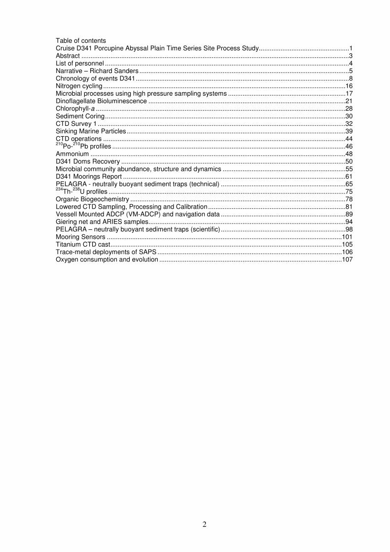
Table of contents Cruise D341 Porcupine Abyssal Plain Time Series Site Process Study..................................................1 Abstract ....................................................................................................................................................3 List of personnel .......................................................................................................................................4 Narrative – Richard Sanders ....................................................................................................................5 Chronology of events D341......................................................................................................................8 Nitrogen cycling ......................................................................................................................................16 Microbial processes using high pressure sampling systems .................................................................17 Dinoflagellate Bioluminescence .............................................................................................................21 Chlorophyll-a ..........................................................................................................................................28 Sediment Coring.....................................................................................................................................30 CTD Survey 1 .........................................................................................................................................32 Sinking Marine Particles.........................................................................................................................39 CTD operations ......................................................................................................................................44 210
Po-210
Pb profiles .................................................................................................................................46 Ammonium .............................................................................................................................................48 D341 Doms Recovery ............................................................................................................................50 Microbial community abundance, structure and dynamics ....................................................................55 D341 Moorings Report ...........................................................................................................................61 PELAGRA - neutrally buoyant sediment traps (technical) .....................................................................65 234
Th-238
U profiles ...................................................................................................................................75 Organic Biogeochemistry .......................................................................................................................78 Lowered CTD Sampling, Processing and Calibration ............................................................................81 Vessell Mounted ADCP (VM-ADCP) and navigation data .....................................................................89 Giering net and ARIES samples.............................................................................................................94 PELAGRA – neutrally buoyant sediment traps (scientific) .....................................................................98 Mooring Sensors ..................................................................................................................................101 Titanium CTD cast................................................................................................................................105 Trace-metal deployments of SAPS ......................................................................................................106 Oxygen consumption and evolution .....................................................................................................107
3
Abstract The Biological Carbon Pump (BCP) is a major feature of the global carbon transporting approximately 10GT C yr
-1 from the ocean surface to the interior mainly via the sinking of particles with an organic
component. The scale of the BCP requires good year-round measurements of its functioning. Moreover, the BCP’s susceptibility to global change means that we need better information on how its climate sensitive elements function and how its poorly parameterised elements operate. These three requirements map directly onto the objectives of this cruise, which will be undertaken using Oceans 2025 funding at the Porcupine Abyssal Plain (PAP) site. The PAP site (47
oN, 16.5
oW) is the location of
a time series of observations from surface to seafloor compiled by IOS, GDD and now NOCS over the last 20 years (Lampitt et al., 2001). A summary of these observations, together with descriptions of surface water biogeochemistry in the region from a cruise in 2005, is currently being published as a special issue of Deep-Sea Research II. The PAP site is close to the site of the JGOFS north Atlantic Bloom experiment and the French POMME programme and is a waypoint on the Atlantic Meridional Transect programme (SO1 in Oceans 2025). There is therefore a rich wealth of previous observations in which our 2009 observations can be grounded. Objectives: 1) To recover and redeploy the PAP site observatory (Theme 10 of Oceans 2025) 2) To compile a vertical carbon budget for the PAP site with particular focus on the process of remineralisation in the mesopelagic (100 – 1000 m) and on the mechanisms leading to export from the upper ocean (Themes 2, 5 of Oceans 2025) 3) To quantify climate sensitive elements of the BCP at the PAP site, particularly the physical processes responsible for introducing nutrients to the upper water column, which combine to set the maximum level of export (Theme 2 of Oceans 2025) Of these, 1) was partially successful, 2) was successful, 3) was unsuccessful.

4
List of personnel Peter Newton Master Richard Warner Chief Officer James Gwinnell Second Officer William McClintock Third Officer Chris Carey Chief Engineer Mark Coultas Second Engineer John Harnett Third Engineer Edin Silajdzic Third Engineer Robert Masters ETO David Hartshorne Purser Michael Drayton Chief Petty Officer - Deck Martin Harrison Chief Perry Offer - Scientific Stuart Cook Petty Officer Deck Gary Crabb Seaman 1A Ian Mills Seaman 1A Peter Smith Seaman 1A Nathaniel Gregory Seaman 1A Duncan Lawes Motorman John Haughton Chef Walter Link Chef Jeffrey Orsborn Steward Anne Robert LMGEM Charlotte Marcinko NOCS Christian Tamburini LMGEM Dominique Lefevre LMGEM Adrian Martin NOCS Athanasios Gritzalis-Papadopoulos NOCS Jennifer Riley NOCS John Allen NOCS Kostas Kiriakoulakis University of Liverpool Nina Rothe NOCS Stuart Painter NOCS Jim Hunter FRS Aberdeen Kevin Saw NOCS Maria Villa University of Seville, Spain Mehdi Boutrif LMGEM Chris Marsay NOCS Frederic Le Moigne NOCS Ian Brown Plymouth Marine Laboratory Mike Zubkov NOCS Peter Statham NOCS Richard Sanders NOCS Ross Holland NOCS Sarah Giering University of Aberdeen Sam Ward NOCS Terry Edwards NOCS Darren Young NOCS Peter Keen Keen Marine Martin Bridger NOCS LMGEM - Laboratoire de Microbiologie Géochimie et Ecologie marine, Marseille NOCS – National Oceanography Centre, Southampton
5
Narrative – Richard Sanders July 2009 9
th Sailed from Govan at noon following the pickup of Sarah Giering and James Hunter from Glasgow
station 10
th On passage
11
th On Passage
12
th On Passage
13
th Work started with a CTD at the future French Mooring position for acoustic release test. The
snowcatcher was deployed followed by another CTD. The weather blew up after the CTD was recovered and the rest of the day was lost. 14
th Work resumed at 9.30. Nets, snowcatchers and Pelagras were deployed at the French mooring
site then CTDs and finally SAPS 15
th Biological work continued till dawn including the French CTD and the French drifter, then the
IODA mooring was deployed. Unfortunately the line linking the release to the instruments parted and approx 700m parafil plus an acoustic release was lost. The remainder of the mooring was recovered. Subsequent tests showed that parafil is slightly negatively buoyant and hence the release can be fired safely some time towards the end of the cruise for recovery. 16
th Aries was deployed around midnight, the French drifter recovered. More biological work ensued
including Snowcatcher, CTD, SAPS. Finally Corer deployment 1 was undertaken which yielded 6 good cores. 17
th More biological work was undertaken and then we embarked on Pelagra recoveries. All were
rounded up in double quick time. The first three were found easily and the other two were slightly more problematic. We then returned to the core site for biological work and coring. 18
th The corer was deployed, PAP 3 was deployed. The French drifter was recovered. The overnight
Aries tow was abandoned due to CLAM problems which were fixed around 4am. Corer deployment 2 19
th IODA was deployed again. This time the deployment was successful. 5 Pelagras were deployed
at the core site. Aries was deployed x 2 20
th DOMS was recovered. The shackle holding the main buoy to the chain had nearly worn through,
the solar panels had nearly all been ripped away. The buoy was sitting low in the water. A number of points have to be addressed before a decision whether to redeploy can be made. We went off to start CTD survey. 21
st CTD survey with occasional nets and snowcatchers
22
nd CTD survey with occasional nets and snowcatchers
23
rd CTD survey with occasional nets and snowcatchers plus SAPS for radiochemists
24
th CTD survey with occasional nets and snowcatchers
25
th CTD survey with occasional nets and snowcatchers
26
th. The final day of the CTD survey. Bad weather prevented work after approximately 9am. Vessel
hove to all day 27
th. Pelagras began to signal their positions at approximately 4am. Two had been caught in a jet and
moved a long way N and three had moved S. By breakfast the sea had abated enough to begin the retrieval process. We ran down to the northerly ones first, recovering the first by about 4PM after 2 failed attempts in which the trap went under the ship. The second was recovered in twilight at about 10PM. We then transited S overnight to look for the second group of traps.
6
28
th. Three Pelagra recoveries were undertaken. The first at approximately noon, the second at
approximately 6 after extensive searching and the third at approximately 10PM. Well coordinated shiphandling and deckwork meant that this difficult task was made to look much simpler that it actually was. We then transited to the coring site 29
th A difficult day. The corer came up with only two poor quality cores. This was followed by a double
ARIES tow, the second of which was brought inboard with the net detached from the codend cartridge. A shallow CTD was undertaken between the tows to allow a large bioluminescence experiment to be initiated. Following the second ARIES tow the Zubkov net was planned to be deployed. Unfortunately the acoustic current meter/ CTD unit which fires the closure mechanisms failed to respond to the computer and the cast was terminated. PAP3 mooring recovered. It came up in something of a tangle and hence the acoustic release was lost although the three traps were all recovered OK with their samples. Next five Pelagras were deployed for recovery on Sunday 2
nd. The French CTD was then
deployed but blew a fuse in the deck unit twice and the cast thus terminated. 30
th This began bright and early with three CTD casts to collect biological samples. Following this the
corer was deployed twice before the weather blew up at around 5PM. The first was successful, the second less so. During the day we conducted final trials on the DOMS toroid and came to the conclusion that the buoyancy available to keep the package out of the water was about 20% of the total buoyancy, possibly due to water ingress. Discussions with base lead to a decision not to redeploy. 31
st Work began at around 9am and stretched out into the rest of the day with CTDs, both French and
English, and the snowcatcher. At about 3PM the decision was made that it was too rough for ARIES to be deployed and so we deployed SAPS before trialling the Zubkov CTD incubator. Unfortunately this completely failed. Nets followed, then deep SAPS. August 2009 1
st The biological station continued with a regular and then the French CTD. The latter had been
revived via a transplant of the titanium housed CTD unit from the trace metal CTD. The French drifter was deployed. Aries was deployed in the afternoon and then again in the evening. 2
nd After Aries the French drifter was located visually and then the CTD deployed with the intention of
drifter recovery thereafter. Unfortunately visual contact with the drifter was lost as the CTD came on board and the weather then blew up and mist came down. Meanwhile by 7am all Pelagras had signalled their positions. Weather downtime from approx 5.30am. By 8 am we had a firm position for the drifter and went off to find the buoy as the weather had come down. The first approach failed and the second resulted in a broken pellet line. The third approach succeeded and we recovered it at 11am. We then set course for the Pelagras in improving (just) weather. Two were sighted straightforwardly and brought in at 2PM and 3PM. The third proved more tricky to spot but was tracked down eventually. Finally two more were recovered between 8 and 10 PM. The biological station could then begin at the site of the last recovery with a French CTD. 3
rd Nets and then two more CTDs ensued before the snowcatcher and finally SAPS were deployed.
Five Pelagras were then deployed at the site of the last recovery and the vessel then departed for a mini CTD survey in the face of an inclement weather forecast. The weather did not blow up and the first station was occupied at 4PM. Further stations at about 7 and 10PM were occupied 4
th A CTD at 3am was followed by a period of awkward confused swells and further CTD deployments
were halted. Vessel still hove to at 2.15. Vessel still hove to at 6.47 the next morning. Wind had dropped and sea abated. 5
th By noon the weather still had not improved enough for over the side work. Swell and wind were
offset meaning station could not be kept. Fortunately the future weather is forecast to be benign. We started stations at about 1PM and then continued them overnight with further stations at approx 4, 7, 10, 1, 4. 6
th Today was devoted to trace metal SAPS for Peter Statham and Chris Marsay, deployed off the
zooplankton winch. A CTD for 234Th
ensued before the hunt for Pelagra began. All five were recovered in 2.5 hours within 5 miles of each other. At one stage there were three showing their lights
7
as a fourth was recovered. We then steamed back to the French Mooring site and deployed the French CTD 7
th The French IODA mooring was recovered today. This was a complex job because it had moved
approximately five miles since deployment due to a light spare anchor being used, the original having been lost when the parafil parted. Fortunately it was just in range standing off the original site and the range decreased as we moved over the top of the original site. We fired the release and then headed off to find it. Triangulation lead to it being sighted just after lunch and it was recovered by teatime. A quick CTD for bioluminescence observations was undertaken and the Zubkov net deployed without its opening/closing device. We then headed for the site where all the Pelagras had been recovered to undertake a biological station to complement the biostation we had occupied immediately prior to the deployment. We towed Aries into the site to obtain a night profile of mesozooplankton biomass and then undertook CTD and SAPS casts overnight followed by two more CTDs. 8
th At noon we redeployed ARIES to replicate the tow from the previous day during the day. Aries was
on board by 6PM and we then set off for the core site. A shallow CTD for instrument calibrations was undertaken and the titanium CTD frame then brought down and assembled. At 10.30 pm we deployed the corer. 9
th The day began well with the corer recovering 8 cores. We then transited to the French mooring
location to recover the lost release. When we ranged the release it didn’t reply coherently but it was clearly there. Intermittent mist meant that it was judged too risky to fire it given the minimal rewards recovering it would bring (no data or instruments were attached to the release) in the expectation that it would trigger despite not communicating sensibly, bearing in mind that the buoyancy package was only two spheres which would lead to it rising slowly and being difficult to spot. We therefore deployed the titanium CTD to 4000m with the hope that firing the release would be possible as the weather improved during the cast. This did not occur and at 10.30 am I took the difficult decision to abandon the French release in favour of obtaining a deep SAPS profile for biochemical analyses at the core site. A string of SAPS were deployed beginning at 12.30 pm and finishing at 7.30PM. A final CTD for bioluminescence experiments was undertaken and with that science at the PAP site ended to allow the core warp to be streamed at reduced speed and the ship departed for home. 10
th On passage
11
th On passage
12
th On passage
13
th Docked
8
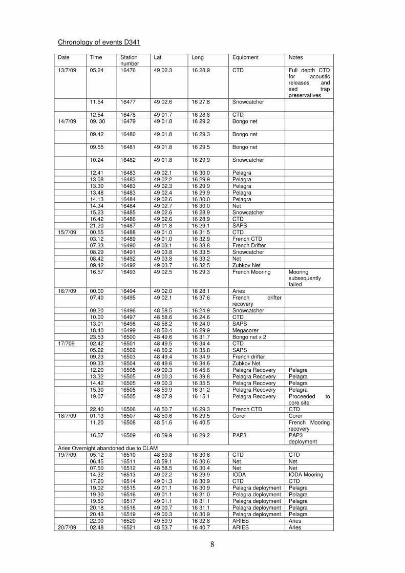
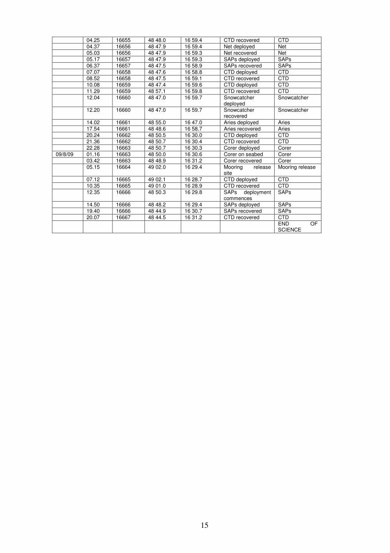
Chronology of events D341 Date Time Station
number Lat Long Equipment Notes
13/7/09 05.24 16476 49 02.3 16 28.9 CTD Full depth CTD for acoustic releases and sed trap preservatives
11.54
16477 49 02.6 16 27.8 Snowcatcher
12.54 16478 49 01.7 16 28.8 CTD 14/7/09 09. 30 16479 49 01.8 16 29.2
Bongo net
09.42 16480 49 01.8 16 29.3
Bongo net
09.55 16481 49 01.8 16 29.5
Bongo net
10.24 16482 49 01.8 16 29.9
Snowcatcher
12.41 16483 49 02.1 16 30.0 Pelagra 13.08 16483 49 02.2 16 29.9 Pelagra 13.30 16483 49 02.3 16 29.9 Pelagra 13.48 16483 49 02.4 16 29.9 Pelagra 14.13 16484 49 02.6 16 30.0 Pelagra 14.34 16484 49 02.7 16 30.0 Net 15.23 16485 49 02.6 16 28.9 Snowcatcher 16.42 16486 49 02.6 16 28.9 CTD 21.20 16487 49 01.8 16 29.1 SAPS 15/7/09 00.55 16488 49 01.0 16 31.5 CTD 03.12 16489 49 01.0 16 32.9 French CTD 07.33 16490 49 03.1 16 33.8 French Drifter 08.29 16491 49 03.8 16 33.5 Snowcatcher 08.42 16492 49 03.8 16 33.2 Net 09.42 16492 49 03.7 16 32.5 Zubkov Net 16.57 16493 49 02.5 16 29.3 French Mooring Mooring
subsequently failed
16/7/09 00.00 16494 49 02.0 16 28.1 Aries 07.40 16495 49 02.1 16 37.6 French drifter
recovery
09.20 16496 48 58.5 16 24.9 Snowcatcher 10.00 16497 48 58.6 16 24.6 CTD 13.01 16498 48 58.2 16 24.0 SAPS 18.40 16499 48 50.4 16 29.9 Megacorer 23.53 16500 48 49.6 16 31.7 Bongo net x 2 17/709 02.42 16501 48 49.5 16 34.4 CTD 05.22 16502 48 50.2 16 35.8 SAPS 09.23 16503 48 49.4 16 34.9 French drifter 09.33 16504 48 49.6 16 34.6 Zubkov Net 12.20 16505 49 00.3 16 45.6 Pelagra Recovery Pelagra 13.32 16505 49 00.3 16 39.8 Pelagra Recovery Pelagra 14.42 16505 49 00.3 16 35.5 Pelagra Recovery Pelagra 15.30 16505 48 59.9 16 31.2 Pelagra Recovery Pelagra 19.07 16505 49 07.9 16 15.1 Pelagra Recovery Proceeded to
core site 22.40 16506 48 50.7 16 29.3 French CTD CTD 18/7/09 01.13 16507 48 50.6 16 29.5 Corer Corer 11.20 16508 48 51.6 16 40.5 French Mooring
recovery 16.57 16509 48 59.9 16 29.2 PAP3 PAP3
deployment Aries Overnight abandoned due to CLAM 19/7/09 05.12 16510 48 59.8 16 30.6 CTD CTD 06.45 16511 48 59.1 16 30.6 Net Net 07.50 16512 48 58.5 16 30.4 Net Net 14.32 16513 49 02.2 16 29.9 IODA IODA Mooring 17.20 16514 49 01.3 16 30.9 CTD CTD 19.02 16515 49 01.1 16 30.9 Pelagra deployment Pelagra 19.30 16516 49 01.1 16 31.0 Pelagra deployment Pelagra 19.50 16517 49 01.1 16 31.1 Pelagra deployment Pelagra 20.18 16518 49 00.7 16 31.1 Pelagra deployment Pelagra 20.43 16519 49 00.3 16 30.9 Pelagra deployment Pelagra 22.00 16520 49 59.9 16 32.8 ARIES Aries 20/7/09 02.48 16521 48 53.7 16 40.7 ARIES Aries
9
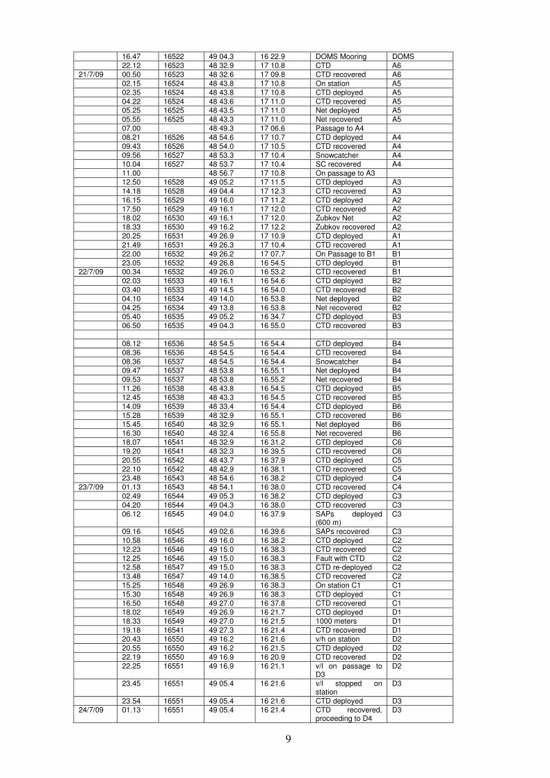
16.47 16522 49 04.3 16 22.9 DOMS Mooring DOMS 22.12 16523 48 32.9 17 10.8 CTD A6 21/7/09 00.50 16523 48 32.6 17 09.8 CTD recovered A6 02.15 16524 48 43.8 17 10.8 On station A5 02.35 16524 48 43.8 17 10.8 CTD deployed A5 04.22 16524 48 43.6 17 11.0 CTD recovered A5 05.25 16525 48 43.5 17 11.0 Net deployed A5 05.55 16525 48 43.3 17 11.0 Net recovered A5 07.00 48 49.3 17 06.6 Passage to A4 08.21 16526 48 54.6 17 10.7 CTD deployed A4 09.43 16526 48 54.0 17 10.5 CTD recovered A4 09.56 16527 48 53.3 17 10.4 Snowcatcher A4 10.04 16527 48 53.7 17 10.4 SC recovered A4 11.00 48 56.7 17 10.8 On passage to A3 12.50 16528 49 05.2 17 11.5 CTD deployed A3 14.18 16528 49 04.4 17 12.3 CTD recovered A3 16.15 16529 49 16.0 17 11.2 CTD deployed A2 17.50 16529 49 16.1 17 12.0 CTD recovered A2 18.02 16530 49 16.1 17 12.0 Zubkov Net A2 18.33 16530 49 16.2 17 12.2 Zubkov recovered A2 20.25 16531 49 26.9 17 10.9 CTD deployed A1 21.49 16531 49 26.3 17 10.4 CTD recovered A1 22.00 16532 49 26.2 17 07.7 On Passage to B1 B1 23.05 16532 49 26.8 16 54.5 CTD deployed B1 22/7/09 00.34 16532 49 26.0 16 53.2 CTD recovered B1 02.03 16533 49 16.1 16 54.6 CTD deployed B2 03.40 16533 49 14.5 16 54.0 CTD recovered B2 04.10 16534 49 14.0 16 53.8 Net deployed B2 04.25 16534 49 13.8 16 53.8 Net recovered B2 05.40 16535 49 05.2 16 34.7 CTD deployed B3 06.50 16535 49 04.3 16 55.0 CTD recovered B3 08.12 16536 48 54.5 16 54.4 CTD deployed B4 08.36 16536 48 54.5 16 54.4 CTD recovered B4 08.36 16537 48 54.5 16 54.4 Snowcatcher B4 09.47 16537 48 53.8 16.55.1 Net deployed B4 09.53 16537 48 53.8 16.55.2 Net recovered B4 11.26 16538 48 43.8 16 54.5 CTD deployed B5 12.45 16538 48 43.3 16 54.5 CTD recovered B5 14.09 16539 48 33.4 16 54.4 CTD deployed B6 15.28 16539 48 32.9 16 55.1 CTD recovered B6 15.45 16540 48 32.9 16 55.1 Net deployed B6 16.30 16540 48 32.4 16 55.8 Net recovered B6 18.07 16541 48 32.9 16 31.2 CTD deployed C6 19.20 16541 48 32.3 16 39.5 CTD recovered C6 20.55 16542 48 43.7 16 37.9 CTD deployed C5 22.10 16542 48 42.9 16 38.1 CTD recovered C5 23.48 16543 48 54.6 16 38.2 CTD deployed C4 23/7/09 01.13 16543 48 54.1 16 38.0 CTD recovered C4 02.49 16544 49 05.3 16 38.2 CTD deployed C3 04.20 16544 49 04.3 16 38.0 CTD recovered C3 06.12 16545 49 04.0 16 37.9 SAPs deployed
(600 m) C3
09.16 16545 49 02.6 16 39.6 SAPs recovered C3 10.58 16546 49 16.0 16 38.2 CTD deployed C2 12.23 16546 49 15.0 16 38.3 CTD recovered C2 12.25 16546 49 15.0 16 38.3 Fault with CTD C2 12.58 16547 49 15.0 16 38.3 CTD re-deployed C2 13.48 16547 49 14.0 16.38.5 CTD recovered C2 15.25 16548 49 26.9 16 38.3 On station C1 C1 15.30 16548 49 26.9 16 38.3 CTD deployed C1 16.50 16548 49 27.0 16 37.8 CTD recovered C1 18.02 16549 49 26.9 16 21.7 CTD deployed D1 18.33 16549 49 27.0 16 21.5 1000 meters D1 19.18 16541 49 27.3 16 21.4 CTD recovered D1 20.43 16550 49 16.2 16 21.6 v/h on station D2 20.55 16550 49 16.2 16 21.5 CTD deployed D2 22.19 16550 49 16.9 16 20.9 CTD recovered D2 22.25 16551 49 16.9 16 21.1 v/l on passage to
D3 D2
23.45 16551 49 05.4 16 21.6 v/l stopped on station
D3
23.54 16551 49 05.4 16 21.6 CTD deployed D3 24/7/09 01.13 16551 49 05.4 16 21.4 CTD recovered,
proceeding to D4 D3
10
02.35 16552 48 54.7 16 21.7 On station D2 D4 02.47 16552 48 54.7 16 21.7 CTD deployed D4 04.15 16552 48 54.7 16 21.5 CTD recovered D4 04.33 16553 48 54.8 16 21.5 Plankton net
deployed D4
04.50 16553 48 54.8 16 21.5 Plankton net recovered
D4
06.27 16554 48 43.9 16 21.7 On CTD station D5 06.33 16554 48 43.9 16 21.7 CTD deployed D5 06.59 16554 48 44.0 16 21.7 1000 meters D5 07.40 16554 48 44.3 16 21.3 CTD recovered D5 09.05 16555 48 33.0 16 21.7 v/h on station D6 D6 09.15 16555 48 32.9 16 21.7 CTD deployed D6 10.31 16555 48 32.6 16 21.7 CTD recovered;
emergency drill D6
11.00 16555 48 32.6 16 21.7 Drill complete; proceeding to E6
D6
12.20 16556 48 33.0 16 05.5 On station E6 E6 12.28 16556 48 33.0 16 05.5 CTD deployed E6 13.41 16556 48 32.8 16 05.9 CTD recovered;
proceeding to E5 E6
15.02 16557 48 43.9 16 05.4 On station E5 E5 15.08 16557 48 43.9 16 05.4 CTD deployed E5 16.38 16557 48 43.9 16 05.4 CTD recovered E5 16.50 16558 48 44.4 16 05.6 Zubkov net
deployed E5
17.05 16558 48 44.4 16 05.6 Zubkov net recovered
E5
18.30 16559 48 54.8 16 05.3 CTD deployed E4 19.00 16559 48 54.9 16 05.2 1000 meters E4 20.00 16559 48 55.0 16 04.7 CTD recovered E4 21.11 16560 49 05.4 16 05.3 v/l on station E3 21.14 16560 49 05.4 16 05.3 CTD deployed E3 22.32 16560 49 05.0 16 04.9 CTD recovered E3 22.50 16560 49 06.3 16 04.9 v/l on passage to
E2 E3
24.00 16561 49 16.3 16 05.3 v/l on site E2 E2 25/7/09 00.10 16561 49 16.3 16 05.3 CTD deployed E2 01.30 16561 49 16.0 16 04.9 CTD recovered;
proceeding to E1 E2
02.47 16562 49 26.8 16 05.3 On station E1 E1 02.54 16562 49 26.8 16 05.3 CTD deployed E1 04.15 16562 49 27.6 16 03.9 CTD recovered E1 04.30 16563 49 27.6 16 03.9 Plankton net
deployed E1
04.50 16563 49 27.8 16 03.9 Plankton net recovered
E1
05.00 16563 49 28.0 16 03.0 To CTD station E1 06.10 16564 49 27.0 15 48.9 On station for CTD F1 06.24 16564 49 27.2 15 48.7 CTD deployed F1 06.46 16564 49 27.4 15 48.3 1000 meters F1 07.30 16564 49 27.9 15 47.8 CTD recovered F1 09.00 16565 49 20.9 15 48.7 v/l on passage to
F2 F1
10.00 16565 49 16.3 15 48.3 On station; weather bound
F2
12.00 16565 49 15.9 15 45.6 Hove to in weather F2 14.50 16565 49 13.7 14 43.6 v/l returning to F2 F2 15.35 16565 49 16.1 15 48.8 v/l back on station F2 16.00 16565 49 16 15 48 No overside work F2 18.00 16565 49 14 15 48 No overside work F2 20.00 16565 49 13 15 49 Hove to adverse
weather F2
24.00 16565 49 11.5 15 53.5 Hove to in heavy weather
F2
26/7/09 04.00 16565 49 11.5 15 59.7 Hove to in heavy weather
F2
05.00 16565 49 11.0 16 01.5 v/l motion too lively for overside work or equipment recovery
F2
07.00 16565 49 09.4 16 04.9 v/l motion too lively for overside work or equipment recovery
F2
08.30 16566 49 09.4 16 04.9 Proceeding to Pelagras
12.00 16566 49 25 15 32.2 Search for Pelagra
11
14.15 16566 49 24.1 15 33.5 P4 sighted 14.45 16566 49 24.1 15 33.5 Recovery attempts
abandoned due to weather
P4
15.55 16566 49 23.7 15 33.8 P4 recovered P4 16.15 16566 49 23.7 15 34.9 Remain hove to;
passage to P2
21.? 16567 49 57.5 15 37.6 On approach P2 21.47 16567 49 57.5 15 37.6 Line on; buoy I/B P2 22.10 16568 49 57.8 15 39.9 CTD deployed CTD 23.14 16568 49 57.8 15 40.2 CTD recovered CTD 24.00 16568 49 57.7 16 41.5 v/l awaiting deck
work complete
27/7/09 00.40 16568 49 57.0 15 43.4 v/l secure; proceeding towards pelagras
02.00 16568 49 49.0 15 52.6 On passage to pelagra
09.00 16568 49 00.6 16 22.1 v/l on passage to P5
11.50 16568 48 41.7 16 35.7 Buoy sighted P5 12.17 16568 48 41.6 16 35.6 P5 recovered 12.30 16568 48 41.6 16 35.6 Proceeding to P7 14.00 16568 48 28.9 16 32.9 On passage to P7 P7 15.20 16568 48 16.6 16 26.7 On location; search
for P7 P7
18.47 16568 48 12.9 16 21.0 P7 recovered P7 19.10 16568 48 13.0 16 21.9 Next pelagra, P6 21.00 16569 48 28.4 16 18.9 On passage to P6 22.00 16569 48 39.1 16 17.4 Sighted P6 22.39 16569 48 39.1 16 17.4 P6 recovered P6 23.44 16569 48 39.6 16 18.2 Passage to core
site
28/7/09 01.30 16570 48 50.5 16 29.9 On location core site
01.42 16570 48 50.5 16 29.9 Corer deployed Core 03.50 16570 48 49.6 16 28.5 Corer at 4700;
reduced to 10m/min Core
03.56 16570 48 49.6 16 28.5 Increase veer to 15 m/min
Core
04.20 16570 48 49.3 16 28.0 On bottom at 5061m wire out; problems with scrolling on coring winch at 4550 m
Core
05.15 16570 48 49.3 16 28.0 4360m wire out Core 05.27 16570 48 49.3 16 28.0 Paying out 4307 m
(wo) to remove gaps in the winch
Core
05.50 16570 48 48.2 16 27.3 Stop at 4934 m (wo); commence recovery
Core
07.50 16570 48 47.0 16 27.2 Corer recovered Core 10.00 16571 48 59.0 16 29.7 v/l stopped for
deployment Aries
10.20 16571 48 58.8 16 30.2 Aries deployed Aries 13.45 16571 48 59.6 16 41.9 Aries recovered Aries 14.23 16572 48 59.7 16 41.7 CTD deployed 14.56 16572 48 59.7 16 41.7 CTD recovered 15.43 16573 48 59.9 16 41.4 Aries deployed Aries 17.25 16573 49 01.0 16 45.8 Scrolled at 1450m Aries 19.05 16573 49 01.9 16 50.0 Recovering Aries Aries 19.10 16573 49 01.9 16 50.0 Aries recovered Aries 19.40 16574 49 01.8 16 49.9 Zubkov net Net 20.45 16574 49 01.1 16 50.2 Net abandoned;
move to deploy Pelagra
21.12 16574 49 01.1 16 50.2 Buoy O/B P2 P2 21.42 16575 49 01.4 16 50.1 Buoy O/B P4 P4 22.00 16576 49 01.1 16 50.0 Buoy O/B P5 P5 22.22 16577 49 01.1 16 50.0 Buoy O/B P6 P6 22.41 16578 49 00.9 16 50.4 Buoy O/B P7 P7 22.41 16578 49 00.9 16 50.4 v/l preparing French
CTD CTD
23.22 16579 49 00.6 16 50.4 CTD deployed CTD 23.37 16579 49 00.5 16 50.6 Problem CTD CTD
12
recovered 29/7/09 00.44 16580 48 59.9 16 51.4 CTD deployed CTD 02.29 16580 48 59.0 16 52.7 CTD recovered CTD 03.06 16581 48 58.9 16 53.2 Net deployed Net 03.29 16581 48 58.9 16 53.2 Net recovered Net 04.15 16582 48 58.8 16 54.5 CTD deployed CTD 04.30 16582 48 58.8 16 54.5 1000 meters CTD 05.22 16582 48 58.7 16 55.3 CTD recovered CTD 05.55 16582 48 58.7 16 55.3 Swell building up;
no overside work
06.15 16583 48 58.8 16 55.9 CTD deployed CTD 06.55 16583 48 58.9 16.56.1 1000 meters CTD 07.42 16583 48 58.9 16 56.4 CTD recovered CTD 08.58 16584 48 59.0 16 56.3 SAP wt deployed SAPs 09.05 16584 48 59.0 16 56.3 (x2) SAP units
deployed SAPs
09.14 16584 48 59.0 16 56.3 + (x2) SAP units deployed
SAPs
12.22 16584 48 49.2 16 56.5 SAPs recovered; proceeding to PAP3
SAPs
14.20 16585 48 58.6 16 27.8 On station PAP3 PAP3 15.00 16585 48 58.2 16 27.2 Release fired PAP3 15.40 16585 48 58.0 16 27.3 PAP3 mooring
sighted PAP3
16.12 16585 48 58.2 16 27.5 Mooring recovery PAP3 16.30 16585 48 58.2 16 27.5 Sediment trap
recovered PAP3
17.00 16585 48 58.2 16 27.5 Sediment trap recovered
PAP3
17.40 16585 48 57.3 16 27.8 Float recovered PAP3 17.45 16585 48 57.3 16 27.8 All recovered PAP3 18.50 16586 48 56.8 16 27.4 French CTD
deployed French CTD
19.06 16586 48 56.7 16 27.4 French CTD recovered (not working)
French CTD
20.23 48 50.6 16 29.5 v/l stopped at core site for CTD or SAPs
SAPs
21.06 16587 48 50.4 16 29.9 SAP wt deployed SAPs 21.18 16587 48 50.4 16 29.9 +1 SAP unit
attached to 400m SAPs
21.34 16587 48 50.4 16 29.9 +1 SAP unit attached to 150m
SAPs
21.43 16587 48 50.4 16 29.9 +1 SAP unit attached to 150m
SAPs
21.52 16587 48 50.4 16 29.9 +1 SAP unit attached to 150 m
SAPs
22.01 16587 48 50.4 16 29.9 +1 SAP unit attached to 150m
SAPs
24.00 16587 48 50.0 16 30.7 v/l holding for SAPs SAPs 30/7/09 00.46 16587 48 49.9 16 30.8 SAP recovery SAPs 02.07 16587 48 49.3 16 30.8 SAP recovered SAPs 02.38 16588 48 49.9 16 30.7 French CTD
deployed French CTD
02.39 16588 48 49.9 16 30.7 CTD recovered due to fault
French CTD
03.19 16588 48 49.9 16 30.7 CTD failed, deployment aborted
French CTD
03.20 16588 48 49.9 16 30.7 Proceeding to coring site
03.30 16588 48 50.7 16 30.0 On location Corer 03.40 16588 48 50.7 16 30.0 Corer deployed Corer 06.00 16588 48 49.6 16 28.6 Stop at 4700m (wo) Corer 06.37 16588 48 49.3 16 28.1 On bottom 5041 m
wo; 5051 wo up Corer
09.28 16588 48 47.9 16 27.3 Corer recovered Corer 10.20 16589 48 47.9 16 27.3 Snowcatcher
deployed Snowcatcher
10.26 16589 48 47.9 16 27.3 Snowcatcher recovered
Snowcatcher
11.11 16590 48 47.9 16 27.6 Corer deployed Corer 13.29 16590 48 47.9 16 27.3 Corer at 4700m;
veering at 10m/min Corer
13.53 16590 48 47.9 16 27.3 Corer on seabed; 4998m wo
Corer
13
15.38 16590 48 48.0 16 26.3 Hauling stopped, crossed wire on drum
Corer
15.42 16590 48 48.0 16 26.3 Fault cleared Corer 16.40 16590 48 47.7 16 25.2 Corer recovered Corer 16.48 16590 48 47.7 16 24.8 Weather
deteriorating; no overside work
18.30 16590 48 46.1 16 23.6 Heavy swell 31/7/09 08.20 16591 48 50.4 16 29.8 French CTD
deployed CTD
11.02 16592 48 49.7 16 30.1 CTD recovered CTD 11.52 16592 48 49.5 16 30.5 CTD deployed CTD 14.10 16592 48 49.2 16 30.8 CTD recovered CTD 15.00 16593 48 49.0 16 30.5 Snowcatcher
deployed Snowcatcher
15.08 16593 48 49.0 16 30.5 Snowcatcher recovered
Snowcatcher
15.27 16594 48 49.0 16 30.4 SAPs deployed (150 m)
SAPs
18.30 16594 48 47.9 16.29.9 SAPs recovered SAPs 19.27 16595 48 47.5 16 30.3 Zubkov CTD
deployed (15 m) Zubkov CTD
21.12 16595 48 46.3 16 30.5 CTD recovered Zubkov CTD 21.58 16596 48 45.9 16 30.9 Giering net
deployed Net
22.12 16596 48 45.9 16 30.9 Net deployed Net 22.14 16596 48 45.9 16 30.9 Net recovered Net 22.24 16596 48 45.9 16 30.9 Net deployed Net 22.25 16596 48 45.9 16 30.9 Net recovered Net 22.31 16596 48 45.9 16 30.9 Net deployed Net 22.33 16596 48 45.9 16 30.9 Net recovered Net 23.08 16596 48 45.9 16 30.9 Net deployed Net 23.34 16597 48 44.9 16 31.4 CTD deployed CTD 01/8/09 00.07 16598 48 44.8 16 31.7 CTD recovered CTD 00.52 16599 48 44.7 16 32.1 SAPs deployed SAPs 01.48 16599 48 44.6 16 32.3 SAPs at 1000 m SAPs 05.07 16599 48 44.1 16 32.5 SAPs recovered SAPs 05.22 16600 48 44.1 16 32.4 Net deployed Net 05.35 16600 48 44.1 16 32.4 Net recovered Net 05.38 16601 48 44.0 16 32.5 Net deployed Net 05.45 16601 48 43.9 16 32.4 Net recovered Net 05.48 16602 48 43.9 16 32.4 Net deployed Net 05.52 16602 48 43.9 16 32.4 Net recovered Net 06.15 16603 48 43 7 16 32.5 Deployment French
drifter Drifter
07.26 16604 48 43.3 16 33.1 CTD deployed CTD 08.46 16604 48 42.5 16 33.2 CTD recovered CTD 09.23 16605 48 42.2 16 33.3 Snowcatcher
deployed Snowcatcher
09.31 16605 48 42.2 16 33.3 Snowcatcher recovered
Snowcatcher
10.08 16606 48 41.8 16 33.4 French CTD deployed
CTD
13.32 16606 48 40.7 16 34.3 CTD recovered CTD 14.20 16607 48 40.7 16 35.1 Aries deployed Aries 18.10 16607 48 40.3 16 49.2 Aries recovered Aries 19.14 16608 48 40.5 16 46.5 Aries deployed Aries 22.45 16608 48 37.3 16 33.3 Aries recovered Aries 02/8/09 01.30 16609 48 38.3 16 33.9 CTD deployed CTD 03.50 16609 48 38.2 16 33.7 CTD recovered CTD 10.54 16610 48 36.6 16 35.5 French drifter
recovered Drifter
13.48 16611 48 47.0 16 51.4 P6 recovered P6 15.00 16612 48 47.6 16 57.7 P5 recovered P5 18.00 16613 48 54.8 17 01.9 P4 recovered P4 21.07 16614 49 04.8 16 31.7 P4 recovered P2 21.45 16615 49 03.4 16 26.4 P7 recovered P7 22.28 16616 49 03.3 16 26.0 French CTD
deployed CTD
03/8/09 00.52 16616 49 02.2 16 26.0 CTD recovered CTD 01.32 16617 49 01.8 16 25.8 Net deployed Net 02.38 16617 49 01.5 16 25.9 Net recovered Net 03.00 16618 49 01.1 16 26.1 CTD deployed CTD 04.20 16618 49 00.2 16 25.7 CTD recovered CTD
14
05.20 16619 48 39.6 16 25.5 CTD deployed CTD 06.55 16619 48 58.6 16 25.5 CTD recovered CTD 07.15 16620 48 58.3 16 25.0 Snowcatcher
deployed Snowcatcher
07.20 16620 48 58.3 16 25.0 SC recovered Snowcatcher 08.09 16621 48 57.9 16 24.5 SAPs deployed SAPs 11.16 16621 48 55.8 16 23.4 SAPs recovered SAPs 12.02 16622 48 55.2 16 23.3 P2 deployed P2 12.28 16623 48 55.1 16 23.3 P4 deployed P4 12.51 16624 48 54.9 16 23.2 P5 deployed P5 13.17 16625 48 54.8 16 23.2 P6 deployed P6 13.42 16626 48 54.8 16 23.4 P7 deployed P7 15.57 16627 48 43.8 16 05.4 CTD deployed CTD 17.15 16627 48 43.0 16 05.3 CTD recovered CTD 19.20 16628 48 43.8 16 21.6 CTD deployed CTD 20.32 16628 48 43.0 16 22.1 CTD recovered CTD 22.32 16629 48 43.8 16 37.8 CTD deployed CTD 23.43 16629 48 43.4 16 38.3 CTD recovered CTD 04/8/09 01.45 16630 48 43.9 16 54.5 CTD deployed CTD 03.28 16630 48 43.4 16 54.8 CTD recovered CTD Adverse weather
conditions 05/8/09 13.05 16631 48 54.8 16 54.4 CTD deployed B4 14.52 16631 48 54.8 16 54.4 CTD recovered B4 16.30 16632 49 05.4 16 34.5 CTD deployed B3 17.50 16632 49 05.1 16 54.1 CTD recovered B3 19.20 16633 49 05.2 16 37.9 CTD deployed C3 20.43 16633 49 05.2 16 37.9 CTD recovered C3 22.07 16634 49 05.3 16 22.1 CTD deployed D3 23.45 16634 49 04.7 16 22.7 CTD recovered D3 06/8/09 01.22 16635 49 05.3 16 05.4 CTD deployed E3 03.18 16635 49 04.2 16 05.3 CTD recovered E3 05.00 16636 48 54.4 16 05.3 CTD deployed E4 06.08 16636 48 53.8 16 05.9 CTD recovered E4 08.48 16637 49 01.5 16 28.0 SAPs deployed SAPs 10.56 16637 49 00.1 16 27.5 SAPs recovered SAPs 11.10 16638 48 59.8 16 27.7 SAPs deployed SAPs 12.55 16638 48 59.8 16 27.7 SAPs recovered SAPs 13.19 16639 48 57.8 16 28.2 SAPs deployed SAPs 15.32 16639 48 55.9 16 29.9 SAPs recovered SAPs 15.48 16640 48 53.8 16 30.1 CTD deployed CTD 18.14 16640 48 33.0 16 32.7 CTD recovered CTD 18.35 16641 48 54.9 16 33.0 Zubkov net
deployed Net
19.00 16641 48 54.9 16 33.4 Zubkov net recovered
Net
21.48 16642 48 50.1 16 58.7 Pelagra recovered P4 22.28 16643 48 47.1 17 01.8 Pelagra recovered P2 23.36 16644 48 48.7 17 01.5 Pelagra recovered P5 07/8/09 00.00 16645 48 49.6 17 01.7 Pelagra recovered P6 00.32 16646 48 50.6 17 03.0 Pelagra recovered P7 03.09 16647 49 02.0 16 29.8 Net deployed Net 03.51 16647 49 01.5 16 29.5 Net recovered Net 04.15 16648 49 00.6 16 29.3 French CTD
deployed French CTD
07.24 16648 48 58.9 16 29.3 French CTD recovered
French CTD
09.17 16649 49 02.1 16 29.2 IODA Transponder deployed
IODA
09.46 16649 49 02.1 16 28.9 Transponder recovered
IODA
13.24 16649 48 56.3 16 32.6 IODA recovery commenced
IODA
16.45 16649 48 54.1 16 32.6 IODA onboard IODA 17.08 16650 48 53.8 16 32.6 CTD deployed CTD 17.12 16650 48 53.7 16 32.6 CTD recovered CTD 17.27 16651 48 53.4 16 32.6 Zubkov net
deployed Net
17.52 16651 48 53.1 16 32.5 Zubkov net recovered
Net
19.40 16652 48 55.9 16 45.8 Aries deployed Aries 23.34 16653 48 48.7 16 57.5 Aries recovered Aries 08/8/09 00.13 16654 48 48.5 16 58.2 SAPs deployed SAPs 03.27 16654 48 48.1 16 59.3 SAPs recovered SAPs 03.52 16655 48 48.1 16 59.3 CTD deployed CTD
15
04.25 16655 48 48.0 16 59.4 CTD recovered CTD 04.37 16656 48 47.9 16 59.4 Net deployed Net 05.03 16656 48 47.9 16 59.3 Net recovered Net 05.17 16657 48 47.9 16 59.3 SAPs deployed SAPs 06.37 16657 48 47.5 16 58.9 SAPs recovered SAPs 07.07 16658 48 47.6 16 58.8 CTD deployed CTD 08.52 16658 48 47.5 16 59.1 CTD recovered CTD 10.08 16659 48 47.4 16 59.6 CTD deployed CTD 11.29 16659 48 57.1 16 59.8 CTD recovered CTD 12.04 16660 48 47.0 16 59.7 Snowcatcher
deployed Snowcatcher
12.20 16660 48 47.0 16 59.7 Snowcatcher recovered
Snowcatcher
14.02 16661 48 55.0 16 47.0 Aries deployed Aries 17.54 16661 48 48.6 16 58.7 Aries recovered Aries 20.24 16662 48 50.5 16 30.0 CTD deployed CTD 21.36 16662 48 50.7 16 30.4 CTD recovered CTD 22.28 16663 48 50.7 16 30.3 Corer deployed Corer 09/8/09 01.16 16663 48 50.0 16 30.6 Corer on seabed Corer 03.42 16663 48 48.9 16 31.2 Corer recovered Corer 05.15 16664 49 02.0 16 29.4 Mooring release
site Mooring release
07.12 16665 49 02.1 16 28.7 CTD deployed CTD 10.35 16665 49 01.0 16 28.9 CTD recovered CTD 12.35 16666 48 50.3 16 29.8 SAPs deployment
commences SAPs
14.50 16666 48 48.2 16 29.4 SAPs deployed SAPs 19.40 16666 48 44.9 16 30.7 SAPs recovered SAPs 20.07 16667 48 44.5 16 31.2 CTD recovered CTD END OF
SCIENCE
16
Nitrogen cycling Ian Brown, PML The objectives were to measure the assimilation of ammonia and nitrate, the regeneration of ammonium and the nitrification of ammonium to nitrate in surface waters at the PAP site focussing on vertical profiles of these N-cycling processes. Samples were collected by either filtration onto GF/F filters for analysis using a stable isotope mass spectrometer or onto SPE cartridges for analysis using HPLC and GCMS. Samples were collected for: NH4
+ regeneration: Either micro/mesozooplankton excretion of NH4
+ or bacterial degradation of
dissolved organic N. The method does not separate the contribution from each of these processes. NH4
+ regeneration rate changes with trophic status of the water mass. It also expresses diel variability
in relation to DVM activity of zooplankton.
NH4+ oxidation: The first step of the nitrification process producing NO2
-. This process may be an
important source of nitrous oxide.
NO2- oxidation: The second step of the nitrification process.
The combination of these experiments should provide a useful insight into N-dynamics within this region. CTD’s stations sampled: 16488, 16501, 16510, 16524, 16532, 16543, 16552, 16562, 16580, 16597, 16609, 16618, 16635 and 16655 Samples were taken for:
1. N-assimilation at 55% 33% 20% 7% and 1% sPAR. Using 15
N-tecniques, the theoretical maximum rate of NO3
-and NH4
+ assimilation (Vmax) and half saturation constant (Ks) will be
determined. 2. NH4
+ regeneration at 55% 33% 20% 7% and 1% sPAR. Using isotope dilution techniques the
rate of NH4+ regeneration will be measured and used to correct NH4
+ assimilation rate data.
3. Nitrification at 55% 33% 20% 7% and 1% sPAR Delivery of results: Results should be available within 6 months of receiving frozen samples.
17
Microbial processes using high pressure sampling systems Mehdi Boutrif & Christian Tamburini (LMGEM) Our main aim during this cruise was to estimate the role of prokaryotes in the degradation of the organic matter in the whole water column with a special emphasis in the meso- and upper bathypelagic waters. To achieve this we used special high-pressure (HP) systems with common units known as high-pressure bottles (HPBs). These were fitted on a Sea-Bird Carousel with Niskin bottles (called thereafter HPSS for High Pressure Serial Sampler) in order to measure in situ prokaryotic activities. They were also used to simulate the pressure that attached microbes experience as they sink through the water column. Hence, during D341 4 tasks were undertaken:
- Task 1 – Prokaryotic structure - Task 2 – Activity in the whole water column - Task 3 – SINking PArticles Simulation - Task 4 – High-pressure bacteria cultivation from deep sediments
Task 1 – Prokaryotic structure Cast number 009, Station 16253 (20 July 09). Depth sampled: 5, 25, 50, 100, 200, 300, 500, 750, 1000, 2000, 3000 m. Different volumes of seawater were sampled. Formalin was added (2% final volume). A subsample was analyzed by flow cytometry by the Zubkov team. After an overnight incubation, samples were filtrated onto 0.2 µm for further analyses at the lab (CARD-FISH, prokaryotic cell counts, biovolume). We sampled particles from PELAGRA at different depth: 50, 150 and 1000m. Further analyses on the RNA and DNA will be done to determine prokaryotes attached to particles. We also sampled particles from SAPS at 150 and 1000m depth on 53µm-pore-size filters and GFF filters. Further analyses will be done in the lab. Finally, we sampled seawater to determine free-living prokaryotes. The ultimate aim is to determine both prokaryotic communities (free-living and attached-to-particles). Task 2 – Prokaryotic activity under in situ conditions This task was closely related to the IODA6000 mooring deployment. Only 6 HPSS were done during the PAP D341 cruise reducing our chance to well validate the results obtained. To increase this, we have finally focused more our attention on the task 2.1 and 2.2. Task 2.1. Heterotrophic prokaryotic production (PHP with
3H-Leu) and Dark CO2 Fixation (DCF)
The aim of this task is to better estimate the PHP (under in situ conditions) in order to have a better estimate prokaryotic carbon demand (PCD) in meso- and bathypelagic waters. For such an aim, we: determined PHP at the same level of IODA6000 incubation: 10, 200, 500, 1000, 2000m-depth.
performed experiments to determine conversion factors for PHP with
3H-leucine: 500, and 2000m-
depth.
sampled to do Micro-CARD-FISH analyses (further in the lab) in order to determine who do what in the meso- and bathypelagic waters. Several profiles have been done during the PAP D341. Analyses have been done on board the ship. Interpretation of these analyses will be done later. Task 2.2. Labile vs semi-labile compounds degradation
18
The aim of this task is to evaluate the capacity of meso- and bathypelagic prokaryotes to degrade semi-labile organic compounds. Indeed, the quality of the organic matter in both environments suggests that prokaryotes have to find their source of carbon and energy in the semi-labile pool of the organic matter. Hence, we have tested their capacities to use exopolysaccharides (EPS) in the meso- and bathypelagic waters. It was the first experiment done in meso- and bathypelagic waters in the Atlantic ocean under in situ pressure and temperature conditions. Several profiles have been done during the PAP D341. Analyses were done on board the ship. Interpretation of these analyses will be done later. Task 2.3. Ectoenzymatic activity (EEA): aminopeptidase (EAA), phosphatase (PA) The aim of this task was to estimate one of the preliminary and obligatory steps that prokaryotes use to degrade high molecular weight DOM to low molecular weight DOM. Fist attempts, in the deep-sea waters of Atlantic Ocean, have been done to determine the effect of pressure on these ectoenzymatic activities. First results obtained during the PAP cruise confirm our previous results in Mediterranean Sea (Tamburini et al., 2003, 2009), i-e., that aminopeptidase and phosphatase activities were higher under in situ pressure conditions than their decompressed counterparts. Task 3 –PArticles Sinking Simulation (PASS) 2 experiments were done, one with the first deployment of the PELAGRA, the other with the second one. SINPAP#1 experiment: The first sinking particles simulation experiment done at the PAP site was done with particles recovered from surface waters and incubated with natural prokaryotic assemblage recovered at 150m-depth. After splitting, particles were incubated over 5 days in 4 HPBs and 4 atmospheric bottles (ATM). Pressure was increased in order to simulate a fall of particles of 200m.d
-1 (for further details
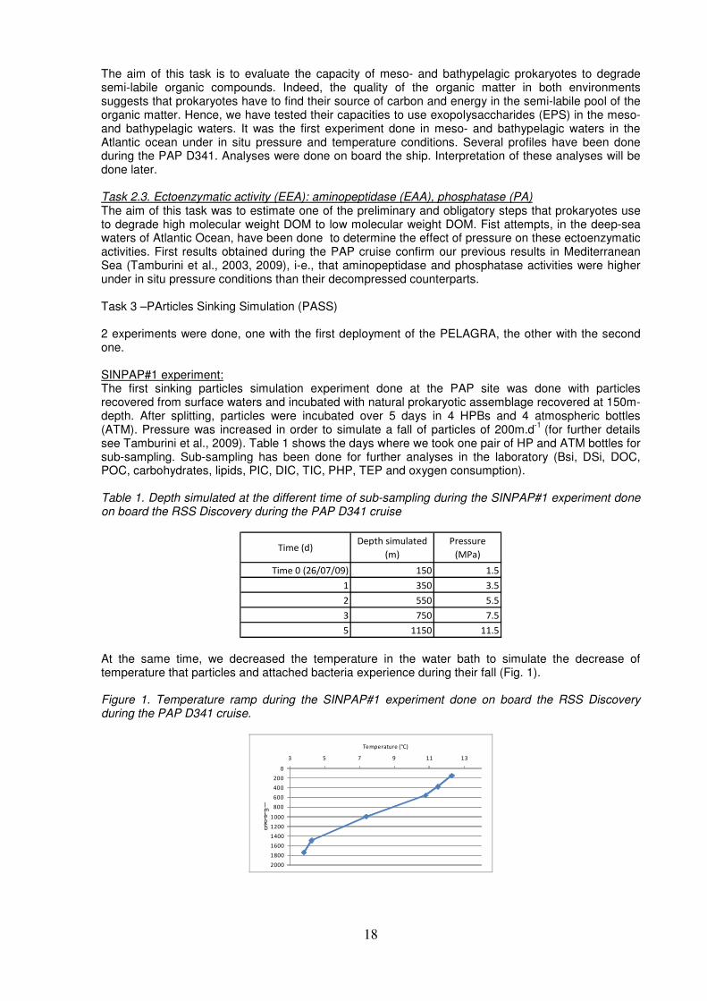
see Tamburini et al., 2009). Table 1 shows the days where we took one pair of HP and ATM bottles for sub-sampling. Sub-sampling has been done for further analyses in the laboratory (Bsi, DSi, DOC, POC, carbohydrates, lipids, PIC, DIC, TIC, PHP, TEP and oxygen consumption). Table 1. Depth simulated at the different time of sub-sampling during the SINPAP#1 experiment done on board the RSS Discovery during the PAP D341 cruise
Time (d)Depth simulated
(m)
Pressure
(MPa)
Time 0 (26/07/09) 150 1.5
1 350 3.5
2 550 5.5
3 750 7.5
5 1150 11.5 At the same time, we decreased the temperature in the water bath to simulate the decrease of temperature that particles and attached bacteria experience during their fall (Fig. 1). Figure 1. Temperature ramp during the SINPAP#1 experiment done on board the RSS Discovery during the PAP D341 cruise.
0
200
400
600
800
1000
1200
1400
1600
1800
2000
3 5 7 9 11 13
Depth (m)
Temperature (°C)
19
Because of lack of communication, the first experiment was done using 150m-depth seawater with particles obtained in surface waters. So, this experiment would be consider more like a test than an experiment attempting to simulate the fall of particles through the mesopelagic waters. SINPAP#2 experiment: The second sinking particles simulation experiment done at the PAP site was undertaken with particles recovered at 50m-depth incubated with a natural prokaryotic assemblage recovered at 50m-depth. After splitting, particles have been incubated during 5 days in 5 HPBs and 5 atmospheric bottles (ATM). Pressure was increased in order to simulate a fall of particles of 200m.d
-1. Table 2 shows the
days where we have taken one pair of HP and ATM bottles for sub-sampling. Sub-sampling has been done for further analyses in the laboratory (Bsi, DSi, DOC, POC, carbohydrates, lipids, PIC, DIC, TIC, PHP, TEP and oxygen consumption). Table 2. Depth simulated at the different time of sub-sampling during the SINPAP#2 experiment done on board the RSS Discovery during the PAP D341 cruise
Time (d)Depth simulated
(m)
Pressure
(MPa)
Time 0 (03/08/09) 50 0.5
1 250 2.5
2 450 4.5
4 850 8.5
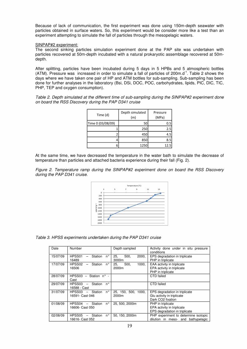
6 1250 12.5 At the same time, we have decreased the temperature in the water bath to simulate the decrease of temperature than particles and attached bacteria experience during their fall (Fig. 2). Figure 2. Temperature ramp during the SINPAP#2 experiment done on board the RSS Discovery during the PAP D341 cruise.
0
200
400
600
800
1000
1200
1400
1600
1800
2000
3 5 7 9 11 13
Depth (m)
Temperature (°C)
Table 3. HPSS experiments undertaken during the PAP D341 cruise
Date Number Depth sampled Activity done under in situ pressure conditions
15/07/09 HPSS01 – Station n° 16489
25, 500, 2000, 3000m
EPS degradation in triplicate PHP in triplicate
17/07/09 HPSS02 – Station n° 16506
25, 500, 1000, 2000m
EAA activity in triplicate EPA activity in triplicate PHP in triplicate
28/07/09 HPSS03 – Station n° - Cast
CTD failed
29/07/09 HPSS03 – Station n° 16588 - Cast
CTD failed
31/07/09 HPSS03 – Station n° 16591- Cast 046
25, 150, 500, 1000, 2000m
EPS degradation in triplicate Glu activity in triplicate Dark CO2 fixation
01/08/09 HPSS04 – Station n° 16606- Cast 050
25, 500, 2000m PHP in triplicate EPA activity in triplicate EPS degradation in triplicate
02/08/09 HPSS05 – Station n° 16616- Cast 052
50, 150, 2000m PHP experiment to determine isotopic dilution in meso- and bathypelagic
20
Task 4 – Prokaryotic structure and activity (under in situ conditions) This experiment was done using 900 ml of sediments recovered at the PAP site during the last coring. Sediments were then mixed with petroleum and incubated under high pressure (45 MPa), at 4°C and in anoxic conditions. The aim of this experiment is to attempt firstly isolation of hydrocarbonoclastic sulfato-bacteria and secondly to evaluate capacity of natural prokaryotic community from the sediments to degrade hydrocarbons under high pressure and low temperature conditions and in anoxic conditions, extreme conditions being an industrial interest. The incubation will be continued in the lab with further analyses. References cited in the text Tamburini, C., Garcin, J., Bianchi, A., 2003. Role of deep-sea bacteria in organic matter mineralization and adaptation to hydrostatic pressure conditions in the NW Mediterranean Sea. Aquatic Microbial Ecology 32 (3), 209-218. Tamburini, C., Garel, M., Al Ali, B., Mérigot, B., Kriwy, P., Charrière, B., Budillon, G., 2009. Distribution and activity of Bacteria and Archaea in the different water masses of the Tyrrhenian Sea. Deep Sea Research II 56, 700-712. Tamburini, C., Goutx, M., Guigue, C., Garel, M., Lefèvre, D., Charrière, B., Sempéré, R., Pepa, S., Peterson, M.L., Wakeham, S., Lee, C., 2009. Effects of hydrostatic pressure on microbial alteration of sinking fecal pellets. Deep-Sea Research II in press.
waters
07/08/09 HPSS06 – Station n° 16648- Cast 066
50, 150, 2000m Dark CO2 fixation Glu activity in triplicate PHP in triplicate (in saturated and low concentration)
21
Dinoflagellate Bioluminescence Charlotte Marcinko, Stuart Painter (NOCS) The objectives of the D341 study were to (1) test new modifications made to the bench top bioluminescence instrument, GLOWtracka; (2) identify whether bioluminescent dinoflagellates are present at the Porcupine Abyssal Plain; (3) assess their horizontal and vertical distribution in the water column; (4) characterise the taxonomic composition of bioluminescent dinoflagellates. Experiments were also carried out to investigate variability in the bioluminescence signal recorded due to either natural controls or the sampling methods used. These experiments were designed to assess whether a circadian clock controls the activity of bioluminescence; investigate the affects of daytime light exposure upon night time bioluminescence and investigate the affects of flow speed through the instrument upon the bioluminescence signal. To meet these objectives a total of 58 CTD casts have been sampled for stimulated bioluminescence and the presence (DNA) of the dinoflagellate luciferase gene. Lugols preserved samples have been collected at all corresponding stations, unless stated, which will be used for microscopic analysis. Measurements were consistently taken from near surface depths (typically 5 m) and a wider range of depths were sampled when water availability and time permitted. Measurements of stimulated bioluminescence were taken using a GLOWtracka bathyphotometer manufactured by the Chelsea Technologies Group which has been modified for bench top use. Our bench top system is designed to provide measurements of stimulated bioluminescence, at a frequency of 1 kHz, from a constant flow of water. The voltage potential recorded can be converted into units of photons cm
-2 sec
-1 using a set calibration equation provided by the manufacturers. Specifically this
apparatus was setup in such a way as to maximise the recording of light emission from any bioluminescent dinoflagellates species that may have been present in a water sample. All data from the instrument were recorded using Agilent VEE release 8.5 software and stored in a comma-separated variables (.csv) format. Data were stored using a standard file naming convention as follows ‘disconnnnn_dddm_vl.csv’ where ‘nnnnn’ was the RRS Discovery instrument deployment number followed by ‘ddd’ which represented the depth of the sample and ‘v’ which represented the sample volume. Cruise D341 provided an opportunity to test modifications made to the bench top GLOWtracka instrument. These included the addition of a flowmeter to measure the flow rate through the instrument and a new larger sample settling chamber. The new settling chamber proved to be considerably more light tight than the original and thus the noise level of the signal was reduced. The larger chamber also made it possible to vary the volume of water sampled. Therefore, enabling the flow rate through the instrument to be varied by increasing or reducing the head of water in the chamber. Replicate Measurements Replicate measurements were made for 2 litre and 4 litre sample volumes in order to calculate the confidence interval in the bioluminescence measurements made (Table 4). Table 4 Sampling information for replicate measurements made for 2 litre and 4 litre sample volumes.
Flow Variation Experiments The affect of flow rate upon the bioluminescence signal was investigated by varying the sample volume run through the GLOWtracka. One, two, three and four litre volumes of water collected from the same depth on the same CTD cast were used for each experiment. The experiments were repeated three times (Table 5).
Station number
Depth (m)
Niskin Bottle Number
Day Of Year
Sample Volume (Litres)
Time Run through Instrument (GMT)
Number of Replicates Run
16592 5 21,20,19 212 2 15:00 10 16592 5 21,20,19 212 2 23:00 10 16609 5 20,21,22 214 4 15:00 10 16609 5 23,24 214 4 23:00 10
22
Table 5. Sampling information for flow variation measurements made for 1, 2, 3 and 4 litre sample volumes.
Biological Sampling Stations Bioluminescence, DNA and microscopy data were collected from a number of over night biological stations which constituted several CTD casts to provide a wide range of biological measurements. Table 6. Overview of cast, niskin bottles and sample depths for measurements of bioluminescence and the collection of samples for molecular and microscopic analysis (those stations marked with * indicates no data for microscopy taken).
CTD Cast Number
Depth (m)
Niskin Bottle Number
CTD Sample Time (GMT)
Day of Year Sample Volume (Litres)
16477* 5, 25 and 100 24, 22 and 14 15:00 194 2 16486* 5, 35 and 125 16, 11 and 3 17:33 195 2 16488 6 and 32 23 and 12 02:07 196 2 and 4 16497* 5, 25 and 50 24, 22 and 20 11:32 197 2 16510 6 and 35 24 and 15 06:10 201 2 16514 6 17 18:30 201 2
CTD Survey 1 Bioluminescence, DNA and microscopy data were collected from all CTD stations during the mesoscale survey which took place between day of year (DOY) 202 and 206 inclusive (Table 4). Samples that were collected from the CTD were stored in blacked out carboys within a darkened area of the constant temperature lab where the temperature was 16 ˚C whilst waiting to be run through the GLOWtracka. Table 7. Overview of CTD cast, niskin bottles and sample depths for measurements of bioluminescence and the collection of samples for molecular and microscopic analysis for mesoscale CTD survey 1.
CTD Cast Number
Depth (m)
Niskin Bottle Number
Day Of Year
CTD Sample Time (GMT)
Sample Volume (Litres)
Number of Replicates Run
16514 5 17 and 18 200 18:30 1 3
16514 5 17 and 18 200 18:30 2 3
16514 5 17 and 18 200 18:30 3 3
16514 5 17 and 18 200 18:30 4 3
16568 5 15 and 16 207 23:15 1 3
16568 5 15 and 16 207 23:15 2 3
16568 5 15 and 16 207 23:15 3 3
16568 5 15 and 16 207 23:15 4 3
16618 5 23 215 04:20 1 1
16618 5 23 215 04:20 2 1
16618 5 23 215 04:20 3 1
16618 5 23 215 04:20 4 1
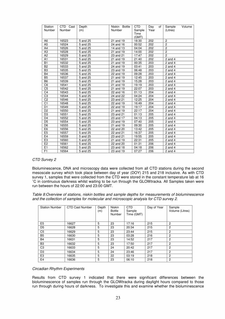
23
CTD Survey 2 Bioluminescence, DNA and microscopy data were collected from all CTD stations during the second mesoscale survey which took place between day of year (DOY) 215 and 218 inclusive. As with CTD survey 1, samples that were collected from the CTD were stored in the constant temperature lab at 16 ˚C in continuous darkness whilst waiting to be run through the GLOWtracka. All Samples taken were run between the hours of 22:00 and 23:00 GMT. Table 8:Overview of stations, niskin bottles and sample depths for measurements of bioluminescence and the collection of samples for molecular and microscopic analysis for CTD survey 2.
Station Number CTD Cast Number Depth (m)
Niskin Bottle Number
CTD Sample Time (GMT)
Day of Year Sample Volume (Litres)
E5 16627 5 23 17:16 215 2
D5 16628 5 23 20:34 215 2
C5 16629 5 23 23:44 215 2
B5 16630 5 23 03:28 216 2
B4 16631 5 23 14:52 217 2
B3 16632 5 23 17:50 217 2
C3 16633 5 24 20:42 217 2
D3 16634 5 24 23:46 217 2
E3 16635 5 22 03:19 218 2
E4 16636 5 23 06:10 218 2
Circadian Rhythm Experiments Results from CTD survey 1 indicated that there were significant differences between the bioluminescence of samples run through the GLOWtracka during daylight hours compared to those run through during hours of darkness. To investigate this and examine whether the bioluminescence
Station Number
CTD Cast Number
Depth (m)
Niskin Bottle Number
CTD Sample Time (GMT)
Day of Year
Sample Volume (Litres)
A6 16523 5 and 25 21 and 19 18:30 202 2 A5 16524 5 and 25 24 and 16 00:52 202 2 A4 16526 5 and 25 14 and 13 04:04 202 2 A3 16528 5 and 25 21 and 19 14:00 202 2 A2 16529 5 and 25 23 and 21 17:47 202 2 A1 16531 5 and 25 21 and 19 21:40 202 2 and 4 B1 16532 5 and 25 21 and 19 00:35 203 2 and 4 B2 16533 5 and 25 24 and 19 03:41 203 2 and 4 B3 16535 5 and 25 23 and 19 06:48 203 2 and 4 B4 16536 5 and 25 22 and 19 09:28 203 2 and 4 B5 16537 5 and 25 21 and 19 12:45 203 2 and 4 B6 16539 5 and 25 21 and 19 15:28 203 2 and 4 C6 16541 5 and 25 21 and 19 19:19 203 2 and 4 C5 16542 5 and 25 21 and 19 22:07 203 2 and 4 C4 16543 5 and 25 22 and 16 01:13 204 2 and 4 C3 16544 5 and 25 24 and 22 04:24 204 2 and 4 C2 16546 5 and 25 23 and 21 12:25 204 2 and 4 C1 16548 5 and 25 22 and 19 16:49 204 2 and 4 D1 16549 5 and 25 22 and 19 19:17 204 2 and 4 D2 16550 5 and 25 21 and 19 22:17 204 2 and 4 D3 16551 5 and 25 23 and 21 01:13 205 2 and 4 D4 16552 5 and 25 23 and 17 04:13 205 2 and 4 D5 16554 5 and 25 23 and 19 07:40 205 2 and 4 D6 16555 5 and 25 21 and 19 09:30 205 2 and 4 E6 16556 5 and 25 22 and 20 13:42 205 2 and 4 E5 16557 5 and 25 22 and 21 16:37 205 2 and 4 E4 16559 5 and 25 23 and 21 19:55 205 2 and 4 E3 16560 5 and 25 21 and 19 22:31 205 2 and 4 E2 16561 5 and 25 22 and 20 01:31 206 2 and 4 E1 16562 5 and 25 23 and 18 04:18 206 2 and 4 F1 16564 5 and 25 23 and 19 07:27 206 2 and 4
24
signal was being affected by the natural circadian rhythms of the organisms producing it, three 48 hour experiments were undertaken. For the first experiment 100 litres of water were collected from CTD cast 16572 at 5 meters depth and a 2 litre sample was run through the GLOWtracka every hour from 16:00 GMT on DOY 208 until 16:00 GMT on DOY 210 (Table 9). Samples for microscopy analysis were taken every 4 hours throughout the 48 hour period and fixed with lugols solution. Water was kept in blacked out carboys within a darkened area of the constant temperature lab where the temperature was 16 ˚C whilst waiting to be run through the GLOWtracka. At the end of the 48 hours spare water was used in a short experiment to investigate the impact of exposure to light on the bioluminescence signal. Eight litres of water was placed in day light for a 7 hour period whilst another 8 litres was continued to be kept in darkness. Bioluminescence measurements were taken hourly from 21:00 (DOY 210) until 00:00 (DOY 211) from both the light exposed and the light deprived water. Preliminary results showed a higher bioluminescence signal in the light exposed compared to the light deprived samples. This was investigated further in the subsequent experiments. Table 9. Sampling information for first circadian rhythm experiment. Measurements made hourly for 48 hours
CTD Cast Number
Sample Number
DOY Sample run Time (GMT)
16572 1 208 16:08
16572 2 208 17:04
16572 3 208 18:03
16572 4 208 19:03
16572 5 208 20:07
16572 6 208 21:04
16572 7 208 22:12
16572 8 208 23:03
16572 9 209 00:04
16572 10 209 01:07
16572 11 209 02:05
16572 12 209 03:08
16572 13 209 04:08
16572 14 209 05:01
16572 15 209 06:01
16572 16 209 07:01
16572 17 209 08:03
16572 18 209 09:02
16572 19 209 10:04
16572 20 209 11:03
16572 21 209 12:04
16572 22 209 13:09
16572 23 209 14:02
16572 24 209 15:04
16572 25 209 16:05
16572 26 209 17:20
16572 27 209 18:03
16572 28 209 19:04
16572 29 209 20:02
16572 30 209 21:05
25
16572 31 209 22:04
16572 32 209 23:0
16572 33 210 00:04
16572 34 210 01:05
16572 35 210 02:06
16572 36 210 03:06
16572 37 210 04:04
16572 38 210 05:00
16572 39 210 06:02
16572 40 210 07:00
16572 41 210 08:00
16572 42 210 09:01
16572 43 210 10:06
16572 44 210 11:08
16572 45 210 12:03
16572 46 210 13:07
16572 47 210 14:04
16572 48 210 15:06
16572 49 210 16:16
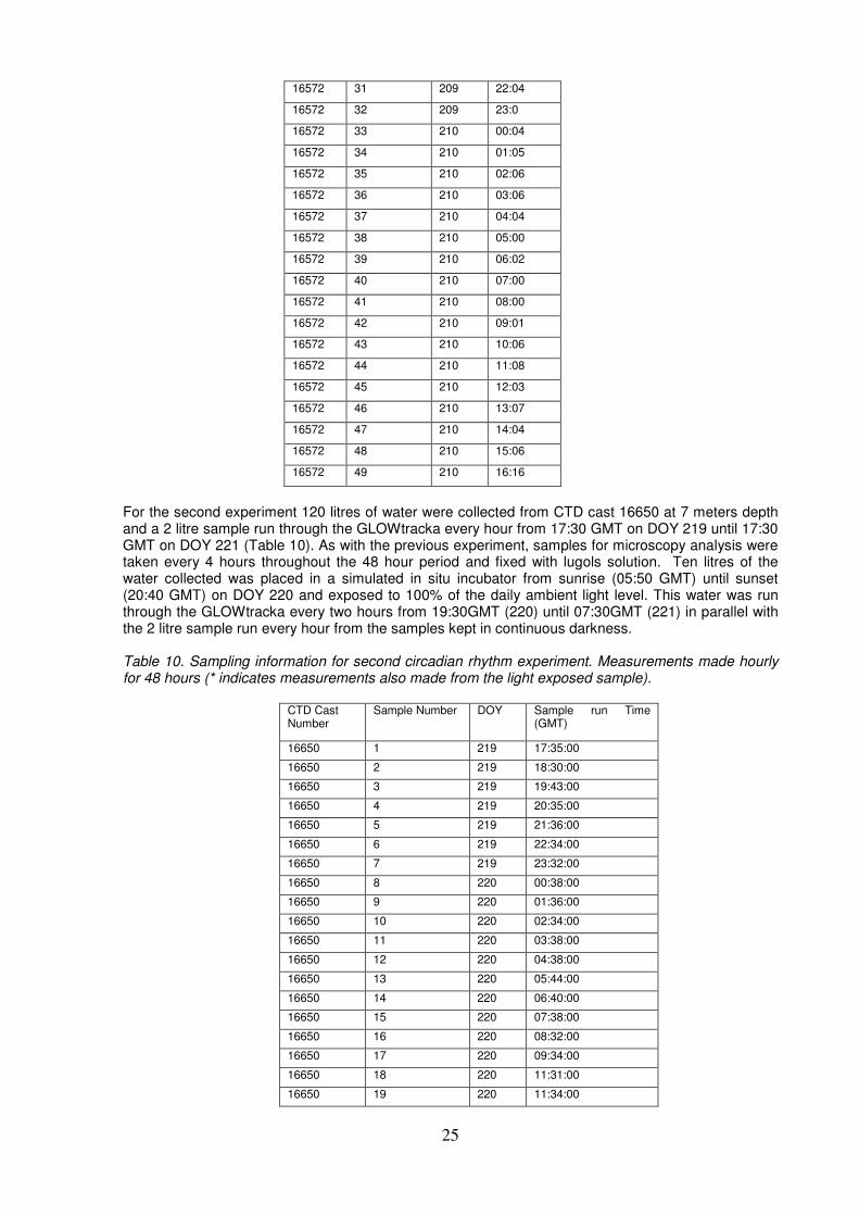
For the second experiment 120 litres of water were collected from CTD cast 16650 at 7 meters depth and a 2 litre sample run through the GLOWtracka every hour from 17:30 GMT on DOY 219 until 17:30 GMT on DOY 221 (Table 10). As with the previous experiment, samples for microscopy analysis were taken every 4 hours throughout the 48 hour period and fixed with lugols solution. Ten litres of the water collected was placed in a simulated in situ incubator from sunrise (05:50 GMT) until sunset (20:40 GMT) on DOY 220 and exposed to 100% of the daily ambient light level. This water was run through the GLOWtracka every two hours from 19:30GMT (220) until 07:30GMT (221) in parallel with the 2 litre sample run every hour from the samples kept in continuous darkness. Table 10. Sampling information for second circadian rhythm experiment. Measurements made hourly for 48 hours (* indicates measurements also made from the light exposed sample).
CTD Cast Number
Sample Number DOY Sample run Time (GMT)
16650 1 219 17:35:00
16650 2 219 18:30:00
16650 3 219 19:43:00
16650 4 219 20:35:00
16650 5 219 21:36:00
16650 6 219 22:34:00
16650 7 219 23:32:00
16650 8 220 00:38:00
16650 9 220 01:36:00
16650 10 220 02:34:00
16650 11 220 03:38:00
16650 12 220 04:38:00
16650 13 220 05:44:00
16650 14 220 06:40:00
16650 15 220 07:38:00
16650 16 220 08:32:00
16650 17 220 09:34:00
16650 18 220 11:31:00
16650 19 220 11:34:00
26
16650 20 220 13:35:00
16650 21 220 14:34:00
16650 22 220 15:35:00
16650 23 220 16:37:00
16650 24 220 17:40:00
16650 25 220 18:50:00
16650 26 220 19:36:00
16650 27 220 20:32:00
16650 28 220 21:30:00
16650 29 220 22:29:00
16650 30 220 23:29:00
16650 31 220 00:35:00
16650 32 221 01:33:00
16650 33 221 02:33:00
16650 34 221 03:36:00
16650 35 221 04:36:00
16650 36 221 05:33:00
16650 37 221 06:33:00
16650 38 221 07:33:00
16650 39 221 08:35:00
16650 40 221 09:35:00
16650 41 221 10:36:00
16650 42 221 11:35:00
16650 43 221 12:30:00
16650 44 221 13:31:00
16650 45 221 14:30:00
16650 46 221 15:34:00
16650 47 221 16:33:00
16650* 48 220 19:43:00
16650* 49 220 22:39:00
16650* 50 221 01:40:00
16650* 51 221 04:45:00
16650* 52 221 07:42:00
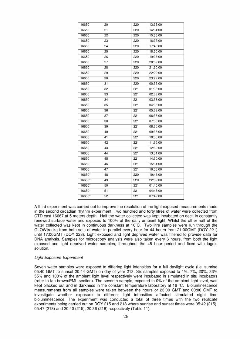
A third experiment was carried out to improve the resolution of the light exposed measurements made in the second circadian rhythm experiment. Two hundred and forty litres of water were collected from CTD cast 16667 at 5 meters depth. Half the water collected was kept incubated on deck in constantly renewed surface water and exposed to 100% of the daily ambient light. Whilst the other half of the water collected was kept in continuous darkness at 16˚C. Two litre samples were run through the GLOWtracka from both sets of water in parallel every hour for 44 hours from 21:00GMT (DOY 221) until 17:00GMT (DOY 223). Light exposed and light deprived water was filtered to provide data for DNA analysis. Samples for microscopy analysis were also taken every 6 hours, from both the light exposed and light deprived water samples, throughout the 48 hour period and fixed with lugols solution. Light Exposure Experiment Seven water samples were exposed to differing light intensities for a full daylight cycle (i.e. sunrise 05:40 GMT to sunset 20:44 GMT) on day of year 213. Six samples exposed to 1%, 7%, 20%, 33% 55% and 100% of the ambient light level respectively were incubated in simulated in situ incubators (refer to Ian brown/PML section). The seventh sample, exposed to 0% of the ambient light level, was kept blacked out and in darkness in the constant temperature laboratory at 16 ˚C. Bioluminescence measurements from all samples were taken between the hours or 23:00 GMT and 00:00 GMT to investigate whether exposure to different light intensities affected stimulated night time bioluminescence. The experiment was conducted a total of three times with the two replicate experiments being carried out on DOY 215 and 218 where sunrise and sunset times were 05:42 (215), 05:47 (218) and 20:40 (215), 20:36 (218) respectively (Table 11).
27
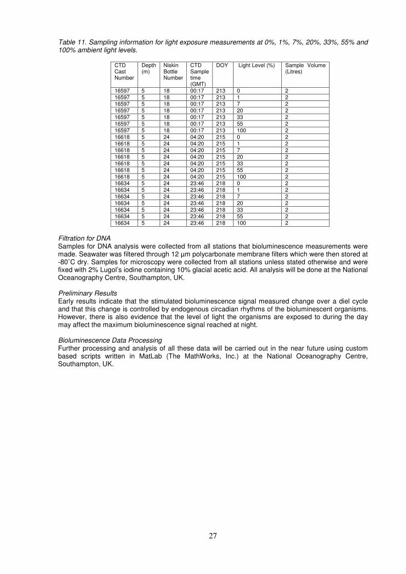
Table 11. Sampling information for light exposure measurements at 0%, 1%, 7%, 20%, 33%, 55% and 100% ambient light levels.
CTD Cast Number
Depth (m)
Niskin Bottle Number
CTD Sample time (GMT)
DOY Light Level (%) Sample Volume (Litres)
16597 5 18 00:17 213 0 2 16597 5 18 00:17 213 1 2 16597 5 18 00:17 213 7 2 16597 5 18 00:17 213 20 2 16597 5 18 00:17 213 33 2 16597 5 18 00:17 213 55 2 16597 5 18 00:17 213 100 2 16618 5 24 04:20 215 0 2 16618 5 24 04:20 215 1 2 16618 5 24 04:20 215 7 2 16618 5 24 04:20 215 20 2 16618 5 24 04:20 215 33 2 16618 5 24 04:20 215 55 2 16618 5 24 04:20 215 100 2 16634 5 24 23:46 218 0 2 16634 5 24 23:46 218 1 2 16634 5 24 23:46 218 7 2 16634 5 24 23:46 218 20 2 16634 5 24 23:46 218 33 2 16634 5 24 23:46 218 55 2 16634 5 24 23:46 218 100 2
Filtration for DNA Samples for DNA analysis were collected from all stations that bioluminescence measurements were made. Seawater was filtered through 12 µm polycarbonate membrane filters which were then stored at -80˚C dry. Samples for microscopy were collected from all stations unless stated otherwise and were fixed with 2% Lugol’s iodine containing 10% glacial acetic acid. All analysis will be done at the National Oceanography Centre, Southampton, UK. Preliminary Results Early results indicate that the stimulated bioluminescence signal measured change over a diel cycle and that this change is controlled by endogenous circadian rhythms of the bioluminescent organisms. However, there is also evidence that the level of light the organisms are exposed to during the day may affect the maximum bioluminescence signal reached at night. Bioluminescence Data Processing Further processing and analysis of all these data will be carried out in the near future using custom based scripts written in MatLab (The MathWorks, Inc.) at the National Oceanography Centre, Southampton, UK.
28
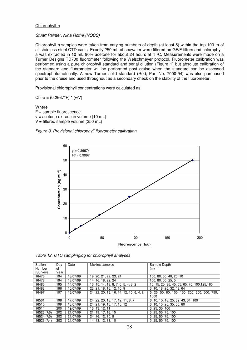
Chlorophyll-a Stuart Painter, Nina Rothe (NOCS) Chlorophyll-a samples were taken from varying numbers of depth (at least 5) within the top 100 m of all stainless steel CTD casts. Exactly 250 mL of seawater were filtered on GF/F filters and chlorophyll-a was extracted in 10 mL 90% acetone for about 24 hours at 4 ºC. Measurements were made on a Turner Designs TD700 fluorometer following the Welschmeyer protocol. Fluorometer calibration was performed using a pure chlorophyll standard and serial dilution (Figure 1) but absolute calibration of the standard and fluorometer will be performed post cruise when the standard can be assessed spectrophotometrically. A new Turner solid standard (Red; Part No. 7000-94) was also purchased prior to the cruise and used throughout as a secondary check on the stability of the fluorometer. Provisional chlorophyll concentrations were calculated as
Chl-a = (0.2667*F) * (v/V) Where F = sample fluorescence v = acetone extraction volume (10 mL) V = filtered sample volume (250 mL) Figure 3. Provisional chlorophyll fluorometer calibration
y = 0.2667x
R2 = 0.9997
0
10
20
30
40
50
60
0 50 100 150 200
Fluorescence (fsu)
Co
ncen
trati
on
(n
g m
l-1)
Table 12. CTD samplinglog for chlorophyll analyses Station Number (Survey)
Day of Year
Date Niskins sampled Sample Depth (m)
16476 194 13/07/09 19, 20, 21, 22, 23, 24 100, 80, 60, 40, 20, 10 16478 194 13/07/09 14, 16, 18, 22, 24 100, 80, 50, 25, 5 16486 195 14/07/09 16, 15, 14, 13, 8, 7, 6, 5, 4, 3, 2 10, 15, 25, 35, 45, 55, 65, 75, 100,125,165 16488 196 15/07/09 23, 21, 18, 16, 12, 10, 9 6, 10, 18, 25, 32, 43, 64 16497 197 16/07/09 24, 22, 20, 18, 16, 14, 12, 10, 6, 4, 2 5, 25, 50, 80, 100, 150, 200, 300, 500, 750,
1000 16501 198 17/07/09 24, 22, 20, 18, 17, 12, 11, 8, 7 6, 10, 15, 18, 25, 32, 43, 64, 100 16510 199 18/07/09 24, 21, 19, 18, 17, 15, 12 6, 10, 15, 25, 35, 50, 80 16514 200 19/07/09 16, 13, 12, 11 6, 25, 30, 100 16523 (A6) 202 21/07/09 21, 19, 17, 16, 15 5, 25, 50, 75, 100 16524 (A5) 202 21/07/09 24, 16, 12, 10, 9 5, 25, 50, 75, 100 16526 (A4) 202 21/07/09 14, 13, 12, 11, 10 5, 25, 50, 75, 100
29
16528 (A3) 202 21/07/09 21, 19, 17, 15, 14 5, 25, 50, 75, 100 16529 (A2) 202 21/07/09 24, 22, 20, 18, 16 5, 25, 50, 75, 100 16531 (A1) 202 21/07/09 21, 19, 17, 15, 13 5, 25, 50, 75, 100 16532 (B1) 203 22/07/09 21, 19, 17, 15, 13 5, 25, 50, 75, 100 16533 (B2) 203 22/07/09 24, 19, 14, 13, 12 5, 25, 50, 75, 100 16535 (B3) 203 22/07/09 23, 19, 17, 15, 13 5, 25, 50, 75, 100 16536 (B4) 203 22/07/09 22, 20, 18, 16, 14 5, 25, 50, 75, 100 16538 (B5) 203 22/07/09 21, 19, 17, 15, 13 5, 25, 50, 75, 100 16539 (B6) 203 22/07/09 21, 19, 17, 15, 13 5, 25, 50, 75, 100 16541 (C6)
203 22/07/09 13, 15, 17, 19, 21 5, 25, 50, 75, 100
16542 (C5)
203 22/07/09 22, 20, 18, 16, 14 5, 25, 50, 75, 100
16543 (C4)
204 23/07/09 22, 16, 12, 11, 10 5, 25, 50, 75, 100
16544 (C3)
204 23/07/09 24, 22, 20, 18, 16 5, 25, 50, 75, 100
16546 (C2)
204 23/07/09 23, 21, 20, 17, 15 5, 25, 50, 75, 100
16548 (C1)
204 23/07/09 22, 20, 17, 15, 14 5, 25, 50, 75, 100
16549 (D1)
204 23/07/09 21, 19, 17, 15, 13 5, 25, 50, 75, 100
16550 (D2)
204 23/07/09 22, 20, 18, 16, 14 5, 25, 50, 75, 100
16551 (D3)
205 24/07/09 22, 20, 18, 15, 13 5, 25, 50, 75, 100
16552 (D4)
205 24/07/09 23, 17, 12, 11, 10 5, 25, 50, 75, 100
16554 (D5)
205 24/07/09 23, 18, 16, 15, 13 5, 25, 50, 75, 100
16555 (D6)
205 24/07/09 22, 20, 18, 16, 14 5, 25, 50, 75, 100
16556 (E6) 205 24/07/09 22, 20, 18, 15, 13 5, 25, 50, 75, 100 16557 (E5) 205 24/07/09 22, 21, 19, 15, 13 5, 25, 50, 75, 100 16559 (E4) 205 24/07/09 23, 21, 19, 18, 15 5, 25, 50, 75, 100 16560 (E3) 205 24/07/09 21, 19, 18, 15, 13 5, 25, 50, 75, 100 16560 (E2) 206 25/07/09 22, 20, 18, 15, 13 5, 25, 50, 75, 100 16562 (E1) 206 25/07/09 23, 18, 11, 10, 9 5, 25, 50, 75, 100 16564 (F1) 206 25/07/09 23, 21, 18, 15, 13 5, 25, 50, 75, 100 16568 207 26/07/09 1, 3, 4, 9, 10, 12, 13, 14, 18 250, 200, 175, 75, 50, 30, 20, 10, 5 16572 209 28/07/09 21, 10, 9, 8, 7, 6, 5, 4, 3, 2, 1 5, 10, 20, 30, 40, 50, 60, 70, 80, 90, 100 16580 210 29/07/09 23, 20, 15, 8, 5 5, 9, 16, 29, 50 16582 210 29/07/09 24, 22, 20, 18 5, 10, 50, 80 16592 212 31/07/09 16, 15, 13, 11, 10 5, 25, 50, 75, 100 16597 213 1/08/09 19, 12, 9, 2, 1 5, 13, 22, 38, 60 16604 213 1/08/09 24, 21, 18, 15 5, 25, 50, 75 16618 215 3/08/09 22, 16, 12, 11, 5, 3, 2 5, 9, 13, 25, 38, 50, 100 16619 215 3/08/09 23, 21, 20, 19, 18, 16, 15 5, 25, 40, 50, 60, 80, 100 16627 (E5) 215 3/08/09 23, 21, 18, 15, 13 5, 25, 50, 75, 100 16628 (D5)
215 3/08/09 22, 20, 18, 16, 14 5, 25, 50, 75, 100
16629 (C5)
216 4/08/09 23, 21, 19, 15, 13 5, 25, 50, 75, 100
16630 (B5) 216 4/08/09 23, 21, 19, 15, 13 5, 25, 50, 75, 100 16631 (B4) 217 5/08/09 23, 21, 19, 15, 13 5, 25, 50, 75, 100 16632 (B3) 217 5/08/09 23, 21, 18, 15, 13 5, 25, 50, 75, 100 16633 (C3)
217 5/08/09 24, 21, 18, 15, 13 5, 25, 50, 75, 100
16634 (D3)
218 6/08/09 23, 21, 19, 16, 13 5, 25, 50, 75, 100
16635 (E3) 218 6/08/09 22, 14, 10, 8, 6 5, 25, 50, 75, 100 16636 (E4) 218 6/08/09 23, 21, 19, 16, 15 5, 25, 50, 75, 100 16640 218 06/08/09 24, 23, 21, 19, 16 5, 25, 50, 75, 100 16655 220 8/08/09 23, 16, 13, 8, 6, 3, 2, 1 5, 18, 25, 38, 42, 60, 75, 100 16658 220 8/08/09 24, 22, 20, 18, 16 5, 25, 50, 75, 100 16662 220 8/08/09 14, 13, 12, 11, 9, 7 5, 10, 20 ,30, 50, 75
30
Sediment Coring Nina Rothe (NOCS) Our goal for D341 was the continuation of the time-series at the Porcupine Abyssal Plain site by observing long-term changes in deep-sea communities in the Northeast Atlantic Ocean. The deep-sea floor is linked intimately to ocean surface processes and rapid, large-scale changes can occur in deep-sea ecosystems. For example, it has been suggested that the North Atlantic Oscillation affects the quantity and quality of carbon exported to the deep sea at the PAP site, which is reflected in changes in abundances observed in all components of the benthic community including meio, macro, and megafauna. On this cruise, undisturbed sediment samples were obtained using a Megacorer. Samples were collected for macrofauna, metazoan meiofauna, and Foraminifera from five deployments (see Table 13). For each deployment, the corer was fitted with eight core tubes of 100 mm internal diameter by 400 mm long (Table 14). The objective was to collect a minimum of three cores for metazoan meiofauna and Foraminifera obtaining one core per deployment. For macrofauna one full sample consists of eight cores from one or two deployments. Table 13. Overview of megacore deployments on D341.
Station ID Date of corer on seabed
Depth (m) oN
oW
16499 16/07/09 4809 48o49.55 16
o30.47
16507 18/07/09 4808 48o49.51 16
o29.95
16570 28/07/09 4808 48o 47.09 16
o27.19
16588 30/07/09 4808 48o49.32 16
o28.13
16590 30/07/09 4808.5 48o47.95 16
o27.19
16663 08/08/09 4808 48o50.72 16
o30.31
Table 14. Station IDs and the number of core tubes deployed and processed after each recovery. F1-F3= Foraminifera samples 1-4; Meio1-4= Meiofauna samples 1-4; Macro1, 2 = Macrofauna samples 1and 2. Sediment height refers to the vertical span of the sediment sampled in each core tube. After each recovery, cores were selected for metazoan meiofauna, Foraminifera, and macrofauna based on an undisturbed sediment surface and a minimum sediment height between 10 and 20 cm. Sediment cores selected for meiofauna and Foraminifera were sectioned down to 5.0 cm in 0.5 cm and 1.0 cm intervals (Table 15). The bottom-water top sediment was first siphoned off and preserved. One core for each faunal group was sectioned down to 10 cm. All sediment was fixed in 10% buffered Formalin. Macrofauna cores were also sectioned down to 5 cm in 1 and 2 cm intervals (Table 3). Prior to fixation, macrofauna samples were split using sieves with mesh sizes 500 µm and 300 µm. Each size group was consequently fixed in 10% buffered formalin.
Station ID
# of cores deployed
# of cores processed
Core IDs Core description (sediment height)
Comments
16499 8 4 1xF1, 1xMeio1, 2xMacro1
F1: 42 cm, Meio1: 41 cm, Macro1: 39 and 40 cm
Little bioturbation
16507 8 6 6xMacro1 Macro1: 40cm, 42cm, 40cm, 42cm, 43cm, 40cm, 40cm
Medium bioturbation
16570 8 2 1xF2, 1xMeio2
F2: 47cm, Meio2: 30 cm
Little bioturbation
16588 8 6 1xF3, 1xMeio3, 4xMacro2
F3: 38cm, Meio3: 37cm, Macro2: 49cm, 50cm, 45cm, 50cm
Strong bioturbation
16590 8 0 - - Bad weather conditions
16663 8 8 1xF4, 1xMeio4, 4xMacro2
F4: 52cm, Meio4: 52cm, Macro2: 52cm, 51cm, 52cm, 51cm
Moderate bioturbation
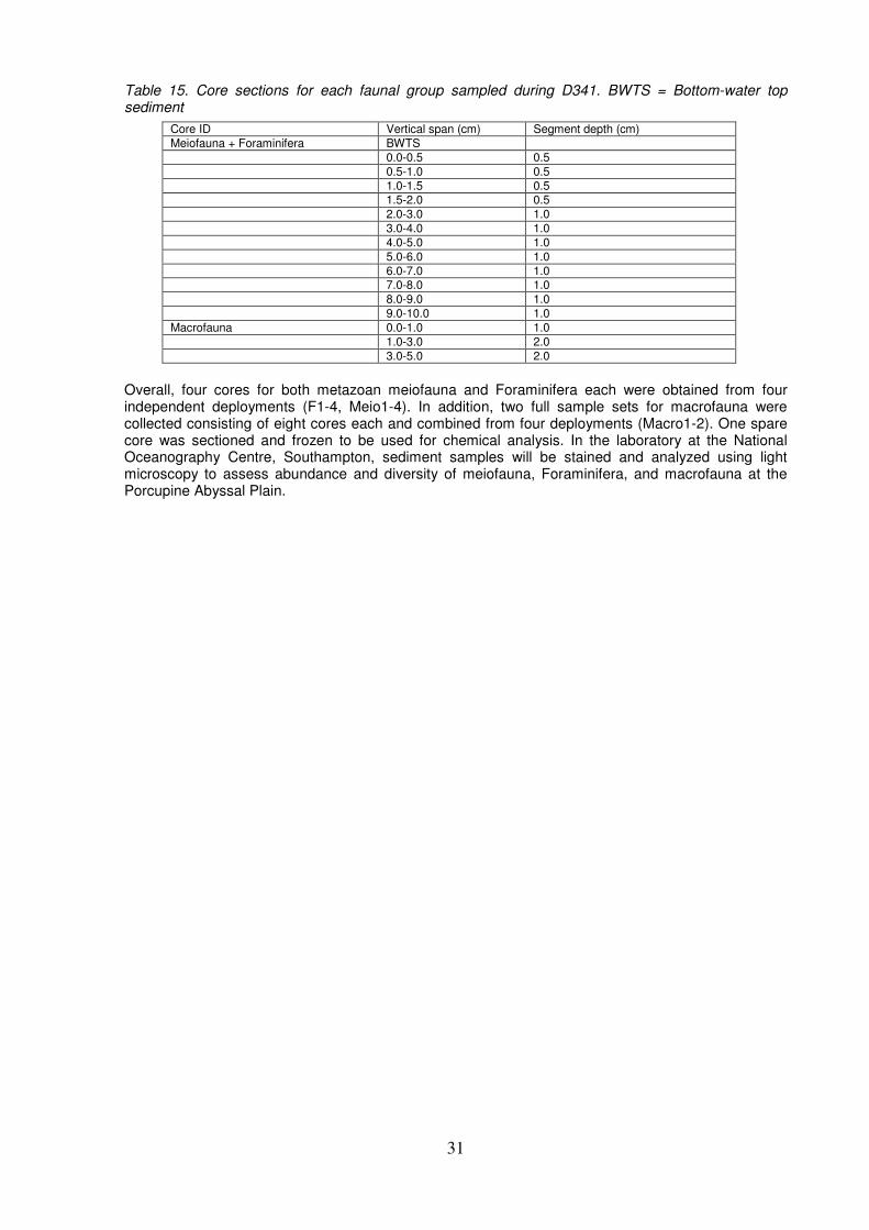
31
Table 15. Core sections for each faunal group sampled during D341. BWTS = Bottom-water top sediment
Overall, four cores for both metazoan meiofauna and Foraminifera each were obtained from four independent deployments (F1-4, Meio1-4). In addition, two full sample sets for macrofauna were collected consisting of eight cores each and combined from four deployments (Macro1-2). One spare core was sectioned and frozen to be used for chemical analysis. In the laboratory at the National Oceanography Centre, Southampton, sediment samples will be stained and analyzed using light microscopy to assess abundance and diversity of meiofauna, Foraminifera, and macrofauna at the Porcupine Abyssal Plain.
Core ID Vertical span (cm) Segment depth (cm) Meiofauna + Foraminifera BWTS 0.0-0.5 0.5 0.5-1.0 0.5 1.0-1.5 0.5 1.5-2.0 0.5 2.0-3.0 1.0 3.0-4.0 1.0 4.0-5.0 1.0 5.0-6.0 1.0 6.0-7.0 1.0 7.0-8.0 1.0 8.0-9.0 1.0 9.0-10.0 1.0 Macrofauna 0.0-1.0 1.0 1.0-3.0 2.0 3.0-5.0 2.0
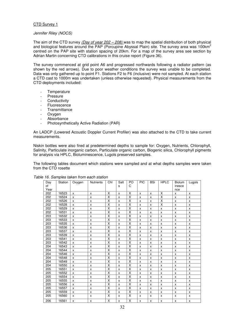
32
CTD Survey 1 Jennifer Riley (NOCS) The aim of the CTD survey (Day of year 202 – 208) was to map the spatial distribution of both physical and biological features around the PAP (Porcupine Abyssal Plain) site. The survey area was 100km
2
centred on the PAP site with station spacing of 20km. For a map of the survey area see section by Adrian Martin concerning CTD calibrations in this cruise report (Figure 36). The survey commenced at grid point A6 and progressed northwards following a radiator pattern (as shown by the red arrows). Due to poor weather conditions the survey was unable to be completed. Data was only gathered up to point F1. Stations F2 to F6 (inclusive) were not sampled. At each station a CTD cast to 1000m was undertaken (unless otherwise requested). Physical measurements from the CTD deployments included:
- Temperature - Pressure - Conductivity - Fluorescence - Transmittance - Oxygen - Absorbance - Photosynthetically Active Radiation (PAR)
An LADCP (Lowered Acoustic Doppler Current Profiler) was also attached to the CTD to take current measurements. Niskin bottles were also fired at predetermined depths to sample for: Oxygen, Nutrients, Chlorophyll, Salinity, Particulate inorganic carbon, Particulate organic carbon, Biogenic silica, Chlorophyll pigments for analysis via HPLC, Bioluminescence, Lugols preserved samples. The following tables document which stations were sampled and at what depths samples were taken from the CTD rosette Table 16. Samples taken from each station
Day of Year
Station Oxygen Nutrients Chl Salts
POC
PIC BSi HPLC Bioluminescence
Lugols
202 16523 x x X x X x x X x x 202 16524 x x X x X x x X x x 202 16526 x x X x X x x X x x 202 16528 x x X x X x x X x x 202 16529 x x X x X x x x x x 202 16531 x x X x X x x x x x 203 16532 x x X x X x x x x x 203 16533 x x X x X x x x x x 203 16535 x x X x X x x x x x 203 16536 x x X x X x x x x x 203 16537 x x X x X x x x x x 203 16539 x x X x X x x x x x 203 16541 x x X x X x x x x x 203 16542 x x X x X x x x x x 204 16543 x x X x X x x x x x 204 16544 x x X x X x x x x x 204 16546 x x X x X x x x x x 204 16548 x x X x X x x x x x 204 16549 x x X x X x x x x x 204 16550 x x X x X x x x x x 205 16551 x x X x X x x x x x 205 16552 x x X x X x x x x x 205 16554 x x X x X x x x x x 205 16555 x x X x X x x x x x 205 16556 x x X x X x x x x x 205 16557 x x X x X x x x x x 205 16559 x x X x X x x x x x 205 16560 x x X x X x x x x x
206 16561 x x X x X x x x x x
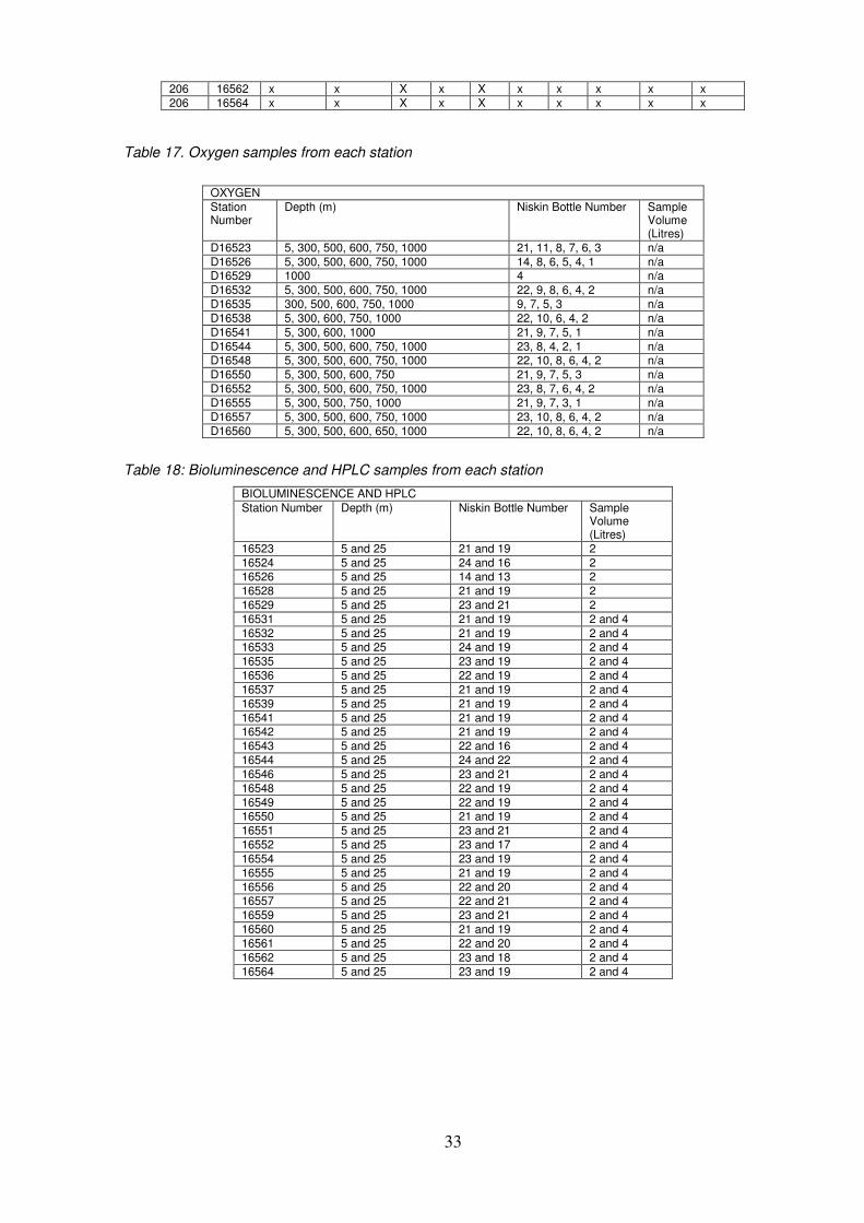
33
Table 17. Oxygen samples from each station Table 18: Bioluminescence and HPLC samples from each station
206 16562 x x X x X x x x x x 206 16564 x x X x X x x x x x
OXYGEN Station Number
Depth (m) Niskin Bottle Number Sample Volume (Litres)
D16523 5, 300, 500, 600, 750, 1000 21, 11, 8, 7, 6, 3 n/a D16526 5, 300, 500, 600, 750, 1000 14, 8, 6, 5, 4, 1 n/a D16529 1000 4 n/a D16532 5, 300, 500, 600, 750, 1000 22, 9, 8, 6, 4, 2 n/a D16535 300, 500, 600, 750, 1000 9, 7, 5, 3 n/a D16538 5, 300, 600, 750, 1000 22, 10, 6, 4, 2 n/a D16541 5, 300, 600, 1000 21, 9, 7, 5, 1 n/a D16544 5, 300, 500, 600, 750, 1000 23, 8, 4, 2, 1 n/a D16548 5, 300, 500, 600, 750, 1000 22, 10, 8, 6, 4, 2 n/a D16550 5, 300, 500, 600, 750 21, 9, 7, 5, 3 n/a D16552 5, 300, 500, 600, 750, 1000 23, 8, 7, 6, 4, 2 n/a D16555 5, 300, 500, 750, 1000 21, 9, 7, 3, 1 n/a D16557 5, 300, 500, 600, 750, 1000 23, 10, 8, 6, 4, 2 n/a D16560 5, 300, 500, 600, 650, 1000 22, 10, 8, 6, 4, 2 n/a
BIOLUMINESCENCE AND HPLC Station Number Depth (m) Niskin Bottle Number Sample
Volume (Litres)
16523 5 and 25 21 and 19 2 16524 5 and 25 24 and 16 2 16526 5 and 25 14 and 13 2 16528 5 and 25 21 and 19 2 16529 5 and 25 23 and 21 2 16531 5 and 25 21 and 19 2 and 4 16532 5 and 25 21 and 19 2 and 4 16533 5 and 25 24 and 19 2 and 4 16535 5 and 25 23 and 19 2 and 4 16536 5 and 25 22 and 19 2 and 4 16537 5 and 25 21 and 19 2 and 4 16539 5 and 25 21 and 19 2 and 4 16541 5 and 25 21 and 19 2 and 4 16542 5 and 25 21 and 19 2 and 4 16543 5 and 25 22 and 16 2 and 4 16544 5 and 25 24 and 22 2 and 4 16546 5 and 25 23 and 21 2 and 4 16548 5 and 25 22 and 19 2 and 4 16549 5 and 25 22 and 19 2 and 4 16550 5 and 25 21 and 19 2 and 4 16551 5 and 25 23 and 21 2 and 4 16552 5 and 25 23 and 17 2 and 4 16554 5 and 25 23 and 19 2 and 4 16555 5 and 25 21 and 19 2 and 4 16556 5 and 25 22 and 20 2 and 4 16557 5 and 25 22 and 21 2 and 4 16559 5 and 25 23 and 21 2 and 4 16560 5 and 25 21 and 19 2 and 4 16561 5 and 25 22 and 20 2 and 4 16562 5 and 25 23 and 18 2 and 4 16564 5 and 25 23 and 19 2 and 4
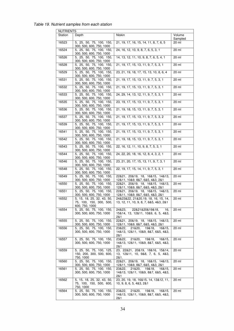
34
Table 19. Nutrient samples from each station
NUTRIENTS Station Depth Niskin Volume
Sampled 16523 5, 25, 50, 75, 100, 150,
300, 500, 600, 750, 1000 21, 19, 17, 16, 15, 14, 11, 8, 7, 6, 5 20 ml
16524 5, 25, 50, 75, 100, 150, 300, 500, 600, 750, 1000
24, 16, 12, 10, 9, 8, 7, 6, 5, 3, 1 20 ml
16526 5, 25, 50, 75, 100, 150, 300, 500, 600, 750, 1000
14, 13, 12, 11, 10, 9, 8, 7, 6, 5, 4, 1 20 ml
16528 5, 25, 50, 75, 100, 150, 300, 500, 600, 750, 1000
21, 19, 17, 15, 13, 11, 9, 7, 5, 3, 1 20 ml
16529 5, 25, 50, 75, 100, 150, 300, 500, 600, 750, 1000
23, 21, 19, 18, 17, 15, 13, 10, 8, 6, 4 20 ml
16531 5, 25, 50, 75, 100, 150, 300, 500, 600, 750, 1000
21, 19, 17, 15, 13, 11, 9, 7, 5, 3, 1 20 ml
16532 5, 25, 50, 75, 100, 150, 300, 500, 600, 750, 1000
21, 19, 17, 15, 13, 11, 9, 7, 5, 3, 1 20 ml
16533 5, 25, 50, 75, 100, 150, 300, 500, 600, 750, 1000
24, 29, 14, 13, 12, 11, 9, 7, 5, 3, 1 20 ml
16535 5, 25, 50, 75, 100, 150, 300, 500, 600, 750, 1000
23, 19, 17, 15, 13, 11, 9, 7, 5, 3, 1 20 ml
16536 5, 25, 50, 75, 100, 150, 300, 500, 600, 750, 1000
21, 19, 18, 15, 13, 11, 9, 7, 5, 3, 1 20 ml
16537 5, 25, 50, 75, 100, 150, 300, 500, 600, 750, 1000
21, 19, 17, 15, 13, 11, 9, 7, 5, 3, 2 20 ml
16539 5, 25, 50, 75, 100, 150, 300, 500, 600, 750, 1000
21, 19, 17, 15, 13, 11, 9, 7, 5, 3, 1 20 ml
16541 5, 25, 50, 75, 100, 150, 300, 500, 600, 750, 1000
21, 19, 17, 15, 13, 11, 9, 7, 5, 3, 1 20 ml
16542 5, 25, 50, 75, 100, 150, 300, 500, 600, 750, 1000
21, 19, 18, 15, 13, 11, 9, 7, 5, 3, 1 20 ml
16543 5, 25, 50, 75, 100, 150, 300, 500, 600, 750, 1000
22, 16, 12, 11, 10, 9, 8, 7, 5, 3, 1 20 ml
16544 5, 25, 50, 75, 100, 150, 300, 500, 600, 750, 1000
24, 22, 20, 18, 16, 12, 8, 4, 3, 2, 1 20 ml
16546 5, 25, 50, 75, 100, 150, 300, 500, 600, 750, 1000
23, 21, 20, 17, 15, 13, 11, 9, 7, 3, 1 20 ml
16548 5, 25, 50, 75, 100, 150, 300, 500, 600, 750, 1000
22, 19, 17, 15, 14, 11, 9, 7, 5, 3, 1 20 ml
16549 5, 25, 50, 75, 100, 150, 300, 500, 600, 750, 1000
22&21, 20&19, 18, 16&15, 14&13, 12&11, 10&9, 8&7, 6&5, 4&3, 2&1
20 ml
16550 5, 25, 50, 75, 100, 150, 300, 500, 600, 750, 1000
22&21, 20&19, 18, 16&15, 14&13, 12&11, 10&9, 8&7, 6&5, 4&3, 2&1
20 ml
16551 5, 25, 50, 75, 100, 150, 300, 500, 600, 750, 1000
22&21, 20&19, 18, 16&15, 14&13, 12&11, 10&9, 8&7, 6&5, 4&3, 2&1
20 ml
16552 5, 15, 18, 25, 32, 43, 50, 75, 100, 150, 300, 500, 600, 750, 1000
24&23&22, 21&20,19, 18, 16, 15, 14, 13, 12, 11, 10, 9, 8, 7, 6&5, 4&3, 2&1
20 ml
16554 5, 25, 50, 75, 100, 150, 300, 500, 600, 750, 1000
24&23, 22&21&20&19&18, 16, 15&14, 13, 12&11, 10&9, 6, 5, 4&3, 2&1
20 ml
16555 5, 25, 50, 75, 100, 150, 300, 500, 600, 750, 1000
22&21, 20&19, 18, 16&15, 14&13, 12&11, 10&9, 8&7, 6&5, 4&3, 2&1
20 ml
16556 5, 25, 50, 75, 100, 150, 300, 500, 600, 750, 1000
23&22, 21&20, 19&18, 16&15, 14&13, 12&11, 10&9, 8&7, 6&5, 4&3, 2&1
20 ml
16557 5, 25, 50, 75, 100, 150, 300, 500, 600, 750, 1000
23&22, 21&20, 19&18, 16&15, 14&13, 12&11, 10&9, 8&7, 6&5, 4&3, 2&1
20 ml
16559 5, 25, 50, 75, 100, 125, 150, 200, 300, 500, 600, 750, 1000
23, 22&21, 20&19, 18&16, 15&14, 13, 12&11, 10, 9&8, 7, 6, 5, 4&3, 2&1.
20 ml
16560 5, 25, 50, 75, 100, 150, 300, 500, 600, 750, 1000
22&21, 20&19, 18, 16&15, 14&13, 12&11, 10&9, 8&7, 6&5, 4&3, 2&1
20 ml
16561 5, 25, 50, 75, 100, 150, 300, 500, 600, 750, 1000
23&22, 21&20, 19&18, 16&15, 14&13, 12&11, 10&9, 8&7, 6&5, 4&3, 2&1
20 ml
16562 5, 15, 18, 25, 32, 43, 50, 75, 100, 150, 500, 600, 750, 1000
23, 20, 19, 18, 16&15, 14, 13&12, 11, 10, 9, 8, 6, 5, 4&3, 2&1
20 ml
16564 5, 25, 50, 75, 100, 150, 300, 500, 600, 750, 1000
23&22, 21&20, 19&18, 16&15, 14&13, 12&11, 10&9, 8&7, 6&5, 4&3, 2&1
20 ml
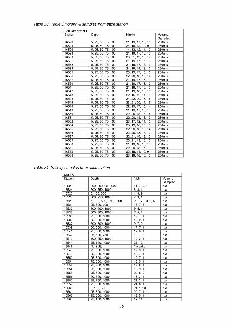
35
Table 20. Table Chlorophyll samples from each station Table 21. Salinity samples from each station
CHLOROPHYLL Station Depth Niskin Volume
Sampled 16523 5, 25, 50, 75, 100 21, 19, 17, 16, 15 250mls 16524 5, 25, 50, 75, 100 24, 16, 12, 10, 9 250mls 16526 5, 25, 50, 75, 100 14, 13, 12, 11, 10 250mls 16528 5, 25, 50, 75, 100 21, 19, 17, 15, 13 250mls 16529 5, 25, 50, 75, 100 23, 21, 19, 18, 17 250mls 16531 5, 25, 50, 75, 100 21, 19, 17, 15, 13 250mls 16532 5, 25, 50, 75, 100 21, 19, 17, 15, 13 250mls 16533 5, 25, 50, 75, 100 24, 19, 14, 13, 12 250mls 16535 5, 25, 50, 75, 100 23, 19, 17, 15, 13 250mls 16536 5, 25, 50, 75, 100 22, 20, 18, 16, 14 250mls 16537 5, 25, 50, 75, 100 21, 19, 17, 15, 13 250mls 16539 5, 25, 50, 75, 100 21, 19, 17, 15, 13 250mls 16541 5, 25, 50, 75, 100 21, 19, 17, 15, 13 250mls 16542 5, 25, 50, 75, 100 21, 19, 18, 15, 13 250mls 16543 5, 25, 50, 75, 100 22, 16, 12, 11, 10 250mls 16544 5, 25, 50, 75, 100 24, 22, 20, 18, 16 250mls 16546 5, 25, 50, 75, 100 23, 21, 20, 17, 15 250mls 16548 5, 25, 50, 75, 100 22, 19, 17, 15, 14 250mls 16549 5, 25, 50, 75, 100 21, 19, 17, 15, 13 250mls 16550 5, 25, 50, 75, 100 22, 20, 18, 16, 14 250mls 16551 5, 25, 50, 75, 100 22, 20, 18, 15, 13 250mls 16552 5, 25, 50, 75, 100 23, 17, 12, 11, 10 250mls 16554 5, 25, 50, 75, 100 23, 19, 16, 15, 13 250mls 16555 5, 25, 50, 75, 100 22, 20, 18, 16, 14 250mls 16556 5, 25, 50, 75, 100 22, 20, 18, 15, 13 250mls 16557 5, 25, 50, 75, 100 22, 21, 19, 15, 13 250mls 16559 5, 25, 50, 75, 100 23, 21, 19, 18, 15 250mls 16560 5, 25, 50, 75, 100 21, 19, 18, 15, 13 250mls 16561 5, 25, 50, 75, 100 22, 20, 18, 15, 13 250mls 16562 5, 25, 50, 75, 100 23, 18, 11, 10, 9 250mls 16564 5, 25, 50, 75, 100 23, 19, 16, 15, 13 250mls
SALTS Station Depth Niskin Volume
Sampled 16523 300, 600, 924, 922 11, 7, 2, 1 n/a 16524 500, 750, 1000 6, 3, 1 n/a 16526 5, 150, 300 1, 8, 9 n/a 16528 500, 750, 1000 7, 3, 1 n/a 16529 5, 100, 500, 750, 1000 23, 17, 10, 6, 4 n/a 16531 75, 500, 600 15, 7, 5 n/a 16532 300, 600, 1000 9, 5, 1 n/a 16533 500, 600, 1000 7, 5, 1 n/a 16535 25, 500, 1000 19, 7, 1 n/a 16536 25, 300, 1000 19, 9, 1 n/a 16537 300, 500, 1000 9, 7, 2 n/a 16539 50, 500, 1000 17, 7, 1 n/a 16541 25, 300, 1000 19, 9, 1 n/a 16542 25, 500, 750 19, 7, 3 n/a 16543 100, 750, 1000 10, 3, 1 n/a 16544 25, 150, 1000 22, 12, 1 n/a 16546 No Salts No salts n/a 16548 25, 300, 1000 19, 9, 1 n/a 16549 25, 500, 1000 19, 7, 1 n/a 16550 25, 500, 1000 19, 7, 1 n/a 16551 75, 600, 1000 15, 5, 1 n/a 16552 25, 300, 1000 17, 8, 1 n/a 16554 25, 300, 1000 19, 9, 1 n/a 16555 25, 500, 1000 20, 8, 2 n/a 16556 50, 750, 1000 18, 3, 1 n/a 16557 25, 750, 1000 21, 3, 1 n/a 16559 25, 500, 1000 21, 6, 1 n/a 16560 5, 150, 500 21, 12, 8 n/a 16561 25, 500, 1000 20, 7, 1 n/a 16562 25, 600, 1000 18, 5, 1 n/a 16564 25, 150, 1000 19, 11, 1 n/a
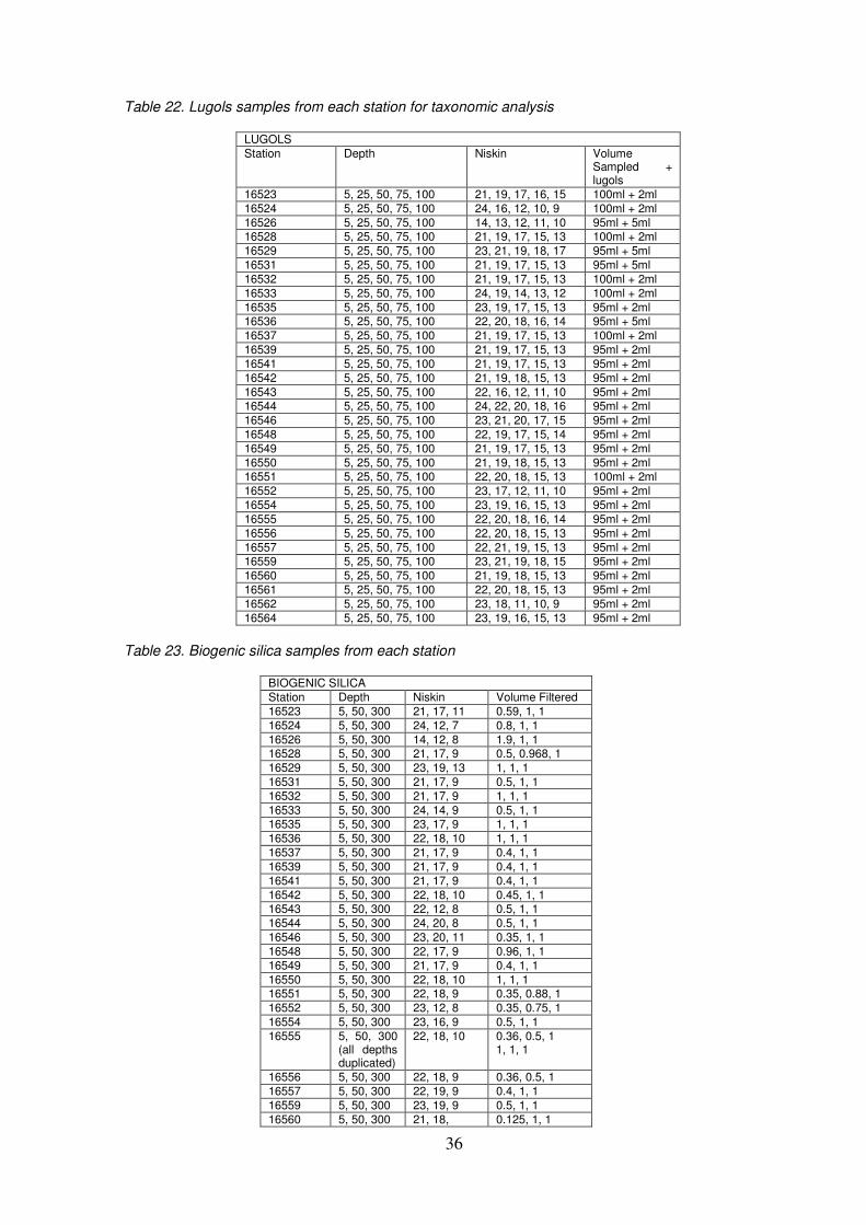
36
Table 22. Lugols samples from each station for taxonomic analysis
LUGOLS Station Depth Niskin Volume
Sampled + lugols
16523 5, 25, 50, 75, 100 21, 19, 17, 16, 15 100ml + 2ml 16524 5, 25, 50, 75, 100 24, 16, 12, 10, 9 100ml + 2ml 16526 5, 25, 50, 75, 100 14, 13, 12, 11, 10 95ml + 5ml 16528 5, 25, 50, 75, 100 21, 19, 17, 15, 13 100ml + 2ml 16529 5, 25, 50, 75, 100 23, 21, 19, 18, 17 95ml + 5ml 16531 5, 25, 50, 75, 100 21, 19, 17, 15, 13 95ml + 5ml 16532 5, 25, 50, 75, 100 21, 19, 17, 15, 13 100ml + 2ml 16533 5, 25, 50, 75, 100 24, 19, 14, 13, 12 100ml + 2ml 16535 5, 25, 50, 75, 100 23, 19, 17, 15, 13 95ml + 2ml 16536 5, 25, 50, 75, 100 22, 20, 18, 16, 14 95ml + 5ml 16537 5, 25, 50, 75, 100 21, 19, 17, 15, 13 100ml + 2ml 16539 5, 25, 50, 75, 100 21, 19, 17, 15, 13 95ml + 2ml 16541 5, 25, 50, 75, 100 21, 19, 17, 15, 13 95ml + 2ml 16542 5, 25, 50, 75, 100 21, 19, 18, 15, 13 95ml + 2ml 16543 5, 25, 50, 75, 100 22, 16, 12, 11, 10 95ml + 2ml 16544 5, 25, 50, 75, 100 24, 22, 20, 18, 16 95ml + 2ml 16546 5, 25, 50, 75, 100 23, 21, 20, 17, 15 95ml + 2ml 16548 5, 25, 50, 75, 100 22, 19, 17, 15, 14 95ml + 2ml 16549 5, 25, 50, 75, 100 21, 19, 17, 15, 13 95ml + 2ml 16550 5, 25, 50, 75, 100 21, 19, 18, 15, 13 95ml + 2ml 16551 5, 25, 50, 75, 100 22, 20, 18, 15, 13 100ml + 2ml 16552 5, 25, 50, 75, 100 23, 17, 12, 11, 10 95ml + 2ml 16554 5, 25, 50, 75, 100 23, 19, 16, 15, 13 95ml + 2ml 16555 5, 25, 50, 75, 100 22, 20, 18, 16, 14 95ml + 2ml 16556 5, 25, 50, 75, 100 22, 20, 18, 15, 13 95ml + 2ml 16557 5, 25, 50, 75, 100 22, 21, 19, 15, 13 95ml + 2ml 16559 5, 25, 50, 75, 100 23, 21, 19, 18, 15 95ml + 2ml 16560 5, 25, 50, 75, 100 21, 19, 18, 15, 13 95ml + 2ml 16561 5, 25, 50, 75, 100 22, 20, 18, 15, 13 95ml + 2ml 16562 5, 25, 50, 75, 100 23, 18, 11, 10, 9 95ml + 2ml 16564 5, 25, 50, 75, 100 23, 19, 16, 15, 13 95ml + 2ml
Table 23. Biogenic silica samples from each station
BIOGENIC SILICA Station Depth Niskin Volume Filtered 16523 5, 50, 300 21, 17, 11 0.59, 1, 1 16524 5, 50, 300 24, 12, 7 0.8, 1, 1 16526 5, 50, 300 14, 12, 8 1.9, 1, 1 16528 5, 50, 300 21, 17, 9 0.5, 0.968, 1 16529 5, 50, 300 23, 19, 13 1, 1, 1 16531 5, 50, 300 21, 17, 9 0.5, 1, 1 16532 5, 50, 300 21, 17, 9 1, 1, 1 16533 5, 50, 300 24, 14, 9 0.5, 1, 1 16535 5, 50, 300 23, 17, 9 1, 1, 1 16536 5, 50, 300 22, 18, 10 1, 1, 1 16537 5, 50, 300 21, 17, 9 0.4, 1, 1 16539 5, 50, 300 21, 17, 9 0.4, 1, 1 16541 5, 50, 300 21, 17, 9 0.4, 1, 1 16542 5, 50, 300 22, 18, 10 0.45, 1, 1 16543 5, 50, 300 22, 12, 8 0.5, 1, 1 16544 5, 50, 300 24, 20, 8 0.5, 1, 1 16546 5, 50, 300 23, 20, 11 0.35, 1, 1 16548 5, 50, 300 22, 17, 9 0.96, 1, 1 16549 5, 50, 300 21, 17, 9 0.4, 1, 1 16550 5, 50, 300 22, 18, 10 1, 1, 1 16551 5, 50, 300 22, 18, 9 0.35, 0.88, 1 16552 5, 50, 300 23, 12, 8 0.35, 0.75, 1 16554 5, 50, 300 23, 16, 9 0.5, 1, 1 16555 5, 50, 300
(all depths duplicated)
22, 18, 10 0.36, 0.5, 1 1, 1, 1
16556 5, 50, 300 22, 18, 9 0.36, 0.5, 1 16557 5, 50, 300 22, 19, 9 0.4, 1, 1 16559 5, 50, 300 23, 19, 9 0.5, 1, 1 16560 5, 50, 300 21, 18, 0.125, 1, 1
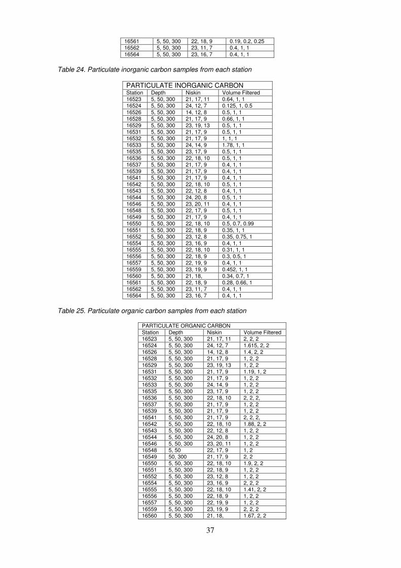
37
16561 5, 50, 300 22, 18, 9 0.19, 0.2, 0.25 16562 5, 50, 300 23, 11, 7 0.4, 1, 1 16564 5, 50, 300 23, 16, 7 0.4, 1, 1
Table 24. Particulate inorganic carbon samples from each station
PARTICULATE INORGANIC CARBON Station Depth Niskin Volume Filtered 16523 5, 50, 300 21, 17, 11 0.64, 1, 1 16524 5, 50, 300 24, 12, 7 0.125, 1, 0.5 16526 5, 50, 300 14, 12, 8 0.5, 1, 1 16528 5, 50, 300 21, 17, 9 0.66, 1, 1 16529 5, 50, 300 23, 19, 13 0.5, 1, 1 16531 5, 50, 300 21, 17, 9 0.5, 1, 1 16532 5, 50, 300 21, 17, 9 1, 1, 1 16533 5, 50, 300 24, 14, 9 1.78, 1, 1 16535 5, 50, 300 23, 17, 9 0.5, 1, 1 16536 5, 50, 300 22, 18, 10 0.5, 1, 1 16537 5, 50, 300 21, 17, 9 0.4, 1, 1 16539 5, 50, 300 21, 17, 9 0.4, 1, 1 16541 5, 50, 300 21, 17, 9 0.4, 1, 1 16542 5, 50, 300 22, 18, 10 0.5, 1, 1 16543 5, 50, 300 22, 12, 8 0.4, 1, 1 16544 5, 50, 300 24, 20, 8 0.5, 1, 1 16546 5, 50, 300 23, 20, 11 0.4, 1, 1 16548 5, 50, 300 22, 17, 9 0.5, 1, 1 16549 5, 50, 300 21, 17, 9 0.4, 1, 1 16550 5, 50, 300 22, 18, 10 0.5, 0.7, 0.99 16551 5, 50, 300 22, 18, 9 0.35, 1, 1 16552 5, 50, 300 23, 12, 8 0.35, 0.75, 1 16554 5, 50, 300 23, 16, 9 0.4, 1, 1 16555 5, 50, 300 22, 18, 10 0.31, 1, 1 16556 5, 50, 300 22, 18, 9 0.3, 0.5, 1 16557 5, 50, 300 22, 19, 9 0.4, 1, 1 16559 5, 50, 300 23, 19, 9 0.452, 1, 1 16560 5, 50, 300 21, 18, 0.34, 0.7, 1 16561 5, 50, 300 22, 18, 9 0.28, 0.66, 1 16562 5, 50, 300 23, 11, 7 0.4, 1, 1 16564 5, 50, 300 23, 16, 7 0.4, 1, 1
Table 25. Particulate organic carbon samples from each station
PARTICULATE ORGANIC CARBON Station Depth Niskin Volume Filtered 16523 5, 50, 300 21, 17, 11 2, 2, 2 16524 5, 50, 300 24, 12, 7 1.615, 2, 2 16526 5, 50, 300 14, 12, 8 1.4, 2, 2 16528 5, 50, 300 21, 17, 9 1, 2, 2 16529 5, 50, 300 23, 19, 13 1, 2, 2 16531 5, 50, 300 21, 17, 9 1.19, 1, 2 16532 5, 50, 300 21, 17, 9 1, 2, 2 16533 5, 50, 300 24, 14, 9 1, 2, 2 16535 5, 50, 300 23, 17, 9 1, 2, 2 16536 5, 50, 300 22, 18, 10 2, 2, 2, 16537 5, 50, 300 21, 17, 9 1, 2, 2 16539 5, 50, 300 21, 17, 9 1, 2, 2 16541 5, 50, 300 21, 17, 9 2, 2, 2, 16542 5, 50, 300 22, 18, 10 1.88, 2, 2 16543 5, 50, 300 22, 12, 8 1, 2, 2 16544 5, 50, 300 24, 20, 8 1, 2, 2 16546 5, 50, 300 23, 20, 11 1, 2, 2 16548 5, 50 22, 17, 9 1, 2 16549 50, 300 21, 17, 9 2, 2 16550 5, 50, 300 22, 18, 10 1.9, 2, 2 16551 5, 50, 300 22, 18, 9 1, 2, 2 16552 5, 50, 300 23, 12, 8 1, 2, 2 16554 5, 50, 300 23, 16, 9 2, 2, 2 16555 5, 50, 300 22, 18, 10 1.41, 2, 2 16556 5, 50, 300 22, 18, 9 1, 2, 2 16557 5, 50, 300 22, 19, 9 1, 2, 2 16559 5, 50, 300 23, 19, 9 2, 2, 2 16560 5, 50, 300 21, 18, 1.67, 2, 2
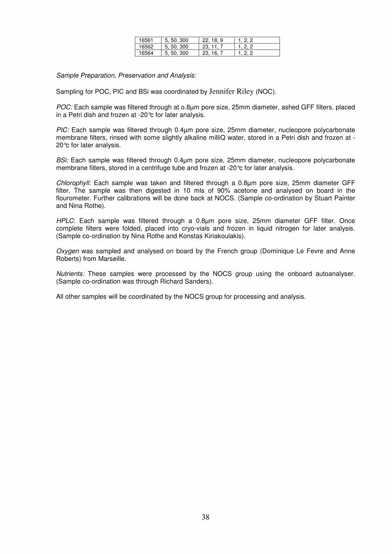
38
16561 5, 50, 300 22, 18, 9 1, 2, 2 16562 5, 50, 300 23, 11, 7 1, 2, 2 16564 5, 50, 300 23, 16, 7 1, 2, 2
Sample Preparation, Preservation and Analysis:
Sampling for POC, PIC and BSi was coordinated by Jennifer Riley (NOC).
POC: Each sample was filtered through at o.8µm pore size, 25mm diameter, ashed GFF filters, placed in a Petri dish and frozen at -20°c for later analysis. PIC: Each sample was filtered through 0.4µm pore size, 25mm diameter, nucleopore polycarbonate membrane filters, rinsed with some slightly alkaline milliQ water, stored in a Petri dish and frozen at -20°c for later analysis. BSi: Each sample was filtered through 0.4µm pore size, 25mm diameter, nucleopore polycarbonate membrane filters, stored in a centrifuge tube and frozen at -20°c for later analysis. Chlorophyll: Each sample was taken and filtered through a 0.8µm pore size, 25mm diameter GFF filter. The sample was then digested in 10 mls of 90% acetone and analysed on board in the flourometer. Further calibrations will be done back at NOCS. (Sample co-ordination by Stuart Painter and Nina Rothe). HPLC: Each sample was filtered through a 0.8µm pore size, 25mm diameter GFF filter. Once complete filters were folded, placed into cryo-vials and frozen in liquid nitrogen for later analysis. (Sample co-ordination by Nina Rothe and Konstas Kiriakoulakis). Oxygen was sampled and analysed on board by the French group (Dominique Le Fevre and Anne Roberts) from Marseille. Nutrients: These samples were processed by the NOCS group using the onboard autoanalyser. (Sample co-ordination was through Richard Sanders). All other samples will be coordinated by the NOCS group for processing and analysis.
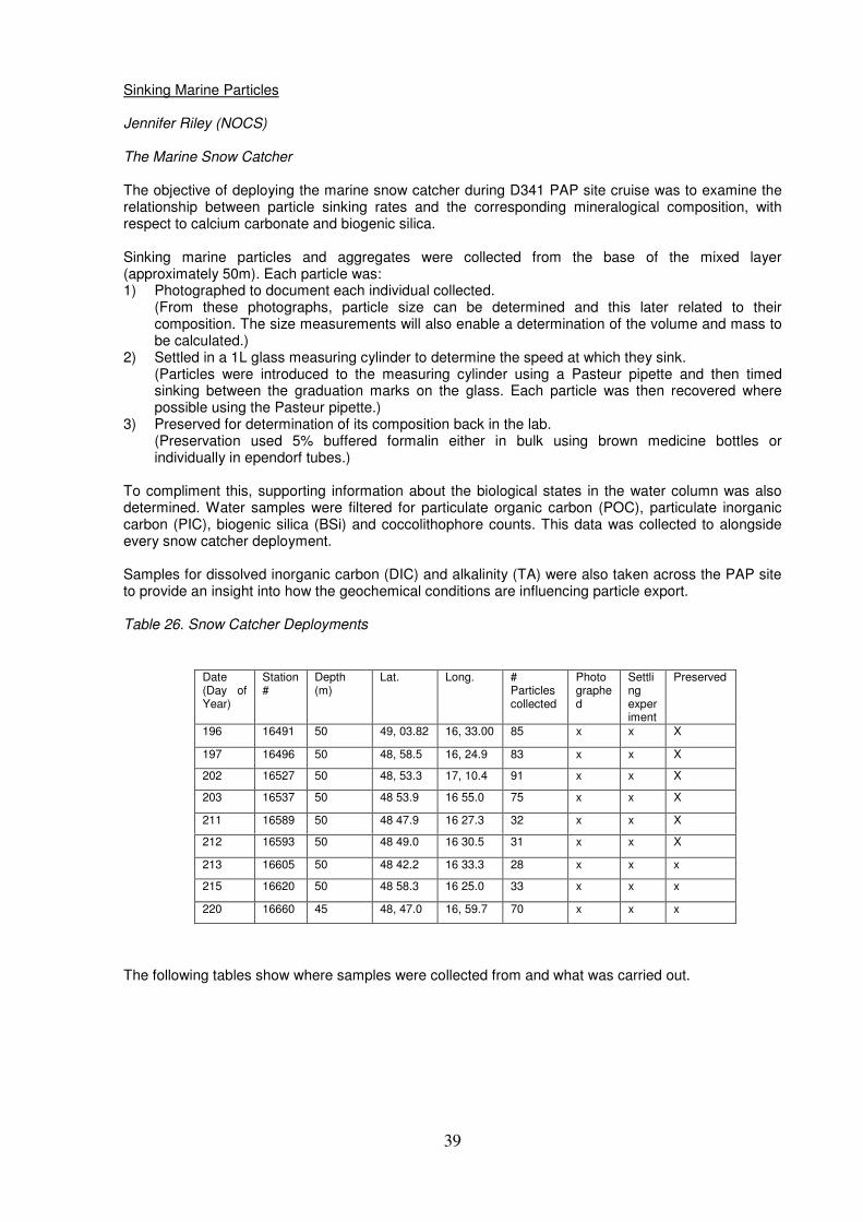
39
Sinking Marine Particles Jennifer Riley (NOCS) The Marine Snow Catcher The objective of deploying the marine snow catcher during D341 PAP site cruise was to examine the relationship between particle sinking rates and the corresponding mineralogical composition, with respect to calcium carbonate and biogenic silica. Sinking marine particles and aggregates were collected from the base of the mixed layer (approximately 50m). Each particle was: 1) Photographed to document each individual collected.
(From these photographs, particle size can be determined and this later related to their composition. The size measurements will also enable a determination of the volume and mass to be calculated.)
2) Settled in a 1L glass measuring cylinder to determine the speed at which they sink. (Particles were introduced to the measuring cylinder using a Pasteur pipette and then timed sinking between the graduation marks on the glass. Each particle was then recovered where possible using the Pasteur pipette.)
3) Preserved for determination of its composition back in the lab. (Preservation used 5% buffered formalin either in bulk using brown medicine bottles or individually in ependorf tubes.)
To compliment this, supporting information about the biological states in the water column was also determined. Water samples were filtered for particulate organic carbon (POC), particulate inorganic carbon (PIC), biogenic silica (BSi) and coccolithophore counts. This data was collected to alongside every snow catcher deployment. Samples for dissolved inorganic carbon (DIC) and alkalinity (TA) were also taken across the PAP site to provide an insight into how the geochemical conditions are influencing particle export. Table 26. Snow Catcher Deployments The following tables show where samples were collected from and what was carried out.
Date (Day of Year)
Station #
Depth (m)
Lat. Long. # Particles collected
Photographed
Settling experiment
Preserved
196 16491 50 49, 03.82 16, 33.00 85 x x X
197 16496 50 48, 58.5 16, 24.9 83 x x X
202 16527 50 48, 53.3 17, 10.4 91 x x X
203 16537 50 48 53.9 16 55.0 75 x x X
211 16589 50 48 47.9 16 27.3 32 x x X
212 16593 50 48 49.0 16 30.5 31 x x X
213 16605 50 48 42.2 16 33.3 28 x x x
215 16620 50 48 58.3 16 25.0 33 x x x
220 16660 45 48, 47.0 16, 59.7 70 x x x
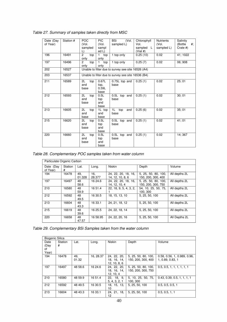
40
Table 27. Summary of samples taken directly from MSC
Table 28. Complementary POC samples taken from water column
Table 29. Complementary BSi Samples taken from the water column
Date (Day of Year)
Station # POC (Vol. sampled L)
PIC (Vol. sampled L)
BSi (Vol. sampled L)
Chlorophyll Vol. sampled L (Vial #)
Nutrients (Vol. sampled L)
Salinity (Bottle #; Crate #)
196 16491 2 top only
1 top only
1 top only 0.25 (10) 0.02 41; 1022
197 16496 2 top only
1 top only
1 top only 0.25 (7) 0.02 06; 908
202 16527 Unable to filter due to survey see site 16526 (A4)
203 16537 Unable to filter due to survey see site 16536 (B4)
211 16589 2L top and base
0.67L top, 0.59L base
0.75L top and base
0.25 (1) 0.02 25; 01
212 16593 2L top and base
0.5L top and base
0.5L top and base
0.25 (1) 0.02 30; 01
213 16605 2L top and base
1L top and base
1L top and base
0.25 (6) 0.02 35; 01
215 16620 2L top and base
0.5L top and base
0.5L top and base
0.25 (1) 0.02 41; 01
220 16660 2L top and base
0.5L top and base
0.5L top and base
0.25 (1) 0.02 14; 367
Particulate Organic Carbon
Date (Day of Year)
Station #
Lat. Long. Niskin Depth
Volume
194 16478 49, 01.328
16, 28.377
24, 22, 20, 18, 16, 14, 12, 10, 8, 6
5, 25, 50, 80, 100, 150, 200, 300, 400
All depths 2L
197 16497 48 58.6
16 24.6 24, 22, 20, 18, 16, 14, 12, 10, 4
5, 25, 50, 80, 100, 150, 200, 300, 750
All depths 2L
210 16580 48 59.9
16 51.4 22, 18, 9, 5, 4, 3, 2, 1
54, 10, 25, 50, 75, 100, 300
All depths 2L
212 16592 48 49.5
16 30.5 18, 15, 13, 10 5, 25, 50, 100 All depths 2L
213 16604 48 43.3
16 33.1 24, 21, 18, 12 5, 25, 50, 100 All depths 2L
215 16619 48 39.6
16 25.5 24, 22, 18, 14 5, 25, 50, 100 All depths 2L
220 16658 48 47.57
16 58.95 24, 22, 20, 16 5, 25, 50, 100 All Depths 2L
Biogenic Silica
Date (Day of Year)
Station #
Lat. Long. Niskin Depth
Volume
194 16478 49, 01.32
16, 28.37 24, 22, 20, 18, 16, 14, 12, 10, 8, 6
5, 25, 50, 80, 100, 150, 200, 300, 400
0.58, 0.56, 1, 0.989, 0.96, 1, 0.89, 0.83, 1
197 16497 48 58.6 16 24.6 24, 22, 20, 18, 16, 14, 12, 10, 4
5, 25, 50, 80, 100, 150, 200, 300, 750
0.5, 0.5, 1, 1, 1, 1, 1, 1
210 16580 48 59.9 16 51.4 22, 18, 9, 5, 4, 3, 2, 1
5, 10, 25, 50, 75, 100, 300
0.43, 0.39, 0.5, 1, 1, 1, 1
212 16592 48 49.5 16 30.5 18, 15, 13, 10
5, 25, 50, 100 0.5, 0.5, 0.5, 1
213 16604 48 43.3 16 33.1 24, 21, 18, 12
5, 25, 50, 100 0.5, 0.5, 1, 1

41
Table 30. Complementary PIC Samples taken from the water column
Table 31. Complementary Coccolithophore Samples taken from the water column
Table 32. Complementary DIC / TA Samples taken from the water column
215 16619 48 39.6 16 25.5 24, 22, 18, 14
5, 25, 50, 100 0.5, 0.5, 0.5, 1
220 16658 48 47.57 16 58.95 24, 22, 20, 16
5, 25, 50, 100 0.5, 0.5, 0.5, 1
Particulate Inorganic Carbon
Date (Day of Year)
Station #
Lat. Long. Niskin Depth
Volume
194 16478
49, 01.328 16, 28.377
24, 22, 20, 18, 16, 14, 12, 10, 8, 6
5, 25, 50, 80, 100, 150, 200, 300, 400
0.89, 0.945, 2, 2, 1, 1, 1, 1, 1
197 16497
48 58.6 16 24.6
24, 22, 20, 18, 16, 14, 12, 10, 4
5, 25, 50, 80, 100, 150, 200, 300, 750
0.39, 0.57, 1, 1, 1, 1, 1, 1
210 16580
48 59.9 16 51.4
22, 18, 9, 5, 4, 3, 2, 1
5, 10, 25, 50, 75, 100, 300
0.5, 0.45, 0.49, 1, 1, 1, 1
212 16592
48 49.5 16 30.5
18, 15, 13, 10 5, 25, 50, 100 0.5, 0.5, 0.5, 1
213 16604
48 43.3 16 33.1
24, 21, 18, 12 5, 25, 50, 100 0.5, 0.5, 1, 1
215 16619
48 39.6 16 25.5
24, 22, 18, 14 5, 25, 50, 100 0.5, 0.5, 0.6, 1
220 16658
48 47.57 16 58.95
24, 22, 20, 16 5, 25, 50, 100 0.5, 0.5, 0.5, 1
Coccolithophores
Date (Day of Year)
Station #
Lat. Long. Niskin Depth
Volume
194 16478 49, 01.32 16, 28.37 24, 22, 20, 18, 16, 14, 12, 10, 8, 6
5, 25, 50, 80, 100 0.5 L all depths
197 16497 48 58.6 16 24.6 24, 22, 20, 18, 16, 14, 12, 10, 4
5, 25, 50, 80, 100, 150, 200, 300, 750
0.1, 0.41, 0.5, 0.5, 0.5
210 16580 48 59.9 16 51.4 22, 18, 9, 5, 4, 3, 2, 1
5, 10, 25, 50, 75, 100
0.5 L all depths
212 16592 48 49.5 16 30.5 18, 15, 13, 10
5, 25, 50, 100 0.5 L all depths
213 16604 48 43.3 16 33.1 24, 21, 18, 12
5, 25, 50, 100 0.5 L all depths
215 16619 48 39.6 16 25.5 24, 22, 18, 14
5, 25, 50, 100 0.5 L all depths
220 16658 48 47.57 16 58.95 24, 22, 20, 16
5, 25, 50, 100 0.5L all depths
DIC/TA Date (Day of Year)
Station # Lat. Long. Niskin Depths Sampled
194 16478 49, 01.328
16, 28.377 5, 25, 50, 80, 100, 200, 400
197 16497 48 58.6
16 24.6 24, 22, 20, 18, 16, 14, 12, 10, 4
5, 25, 50, 80, 100, 150, 200, 300, 750
210 16580 48 59.9
16 51.4 5, 10, 25, 50, 75, 100, 150, 300
217 16631 48, 54.8
16, 59.7 1, 3, 7, 9, 11, 13, 19, 21, 23
1000, 750, 500, 300, 150, 100, 50, 25, 5
217 16634 49, 04.7
16, 22.7 5, 7, 9, 11, 13, 15, 19, 21, 23
600, 500, 300, 150, 100, 75, 50, 25, 5
220 16658 48 47.57
16 58.95 24, 22, 20, 16, 14, 13, 10, 8
5, 25, 50, 100, 150, 300, 450, 600
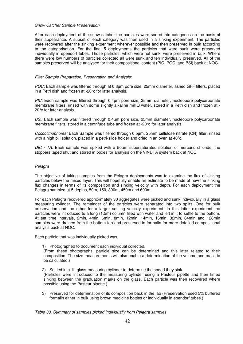
42
Snow Catcher Sample Preservation After each deployment of the snow catcher the particles were sorted into categories on the basis of their appearance. A subset of each category was then used in a sinking experiment. The particles were recovered after the sinking experiment wherever possible and then preserved in bulk according to the categorisation. For the final 5 deployments the particles that were sunk were preserved individually in ependorf tubes. Those particles, which were not sunk, were preserved in bulk. Where there were low numbers of particles collected all were sunk and ten individually preserved. All of the samples preserved will be analysed for their compositional content (PIC, POC, and BSi) back at NOC. Filter Sample Preparation, Preservation and Analysis: POC: Each sample was filtered through at 0.8µm pore size, 25mm diameter, ashed GFF filters, placed in a Petri dish and frozen at -20°c for later analysis. PIC: Each sample was filtered through 0.4µm pore size, 25mm diameter, nucleopore polycarbonate membrane filters, rinsed with some slightly alkaline milliQ water, stored in a Petri dish and frozen at -20°c for later analysis. BSi: Each sample was filtered through 0.4µm pore size, 25mm diameter, nucleopore polycarbonate membrane filters, stored in a centrifuge tube and frozen at -20°c for later analysis. Coccolithophores: Each Sample was filtered through 0.5µm, 25mm cellulose nitrate (CN) filter, rinsed with a high pH solution, placed in a petri-slide holder and dried in an oven at 40ºc. DIC / TA: Each sample was spiked with a 50µm supersaturated solution of mercuric chloride, the stoppers taped shut and stored in boxes for analysis on the VINDTA system back at NOC. Pelagra The objective of taking samples from the Pelagra deployments was to examine the flux of sinking particles below the mixed layer. This will hopefully enable an estimate to be made of how the sinking flux changes in terms of its composition and sinking velocity with depth. For each deployment the Pelagra sampled at 5 depths, 50m, 150, 300m, 450m and 600m. For each Pelagra recovered approximately 30 aggregates were picked and sunk individually in a glass measuring cylinder. The remainder of the particles were separated into two splits. One for bulk preservation and the other for a larger settling velocity experiment. In this latter experiment the particles were introduced to a long (1.5m) column filled with water and left in it to settle to the bottom. At set time intervals, 2min, 4min, 6min, 8min, 12min, 14min, 16min, 32min, 64min and 128min samples were drained from the bottom tap and preserved in formalin for more detailed compositional analysis back at NOC. Each particle that was individually picked was,
1) Photographed to document each individual collected. (From these photographs, particle size can be determined and this later related to their composition. The size measurements will also enable a determination of the volume and mass to be calculated.)
2) Settled in a 1L glass-measuring cylinder to determine the speed they sink. (Particles were introduced to the measuring cylinder using a Pasteur pipette and then timed sinking between the graduation marks on the glass. Each particle was then recovered where possible using the Pasteur pipette.)
3) Preserved for determination of its composition back in the lab (Preservation used 5% buffered formalin either in bulk using brown medicine bottles or individually in ependorf tubes.)
Table 33. Summary of samples picked individually from Pelagra samples
43
* Sample had a jellyfish in it and so was immediately preserved with formalin. However this caused the particles to sink faster in the individual settling experiments due to the different density liquids. Therefore the experiment was abandoned. n.b. For the first two Pelagra pots particles were not preserved individually but bulked together. The rest of the Pelagra samples had 30 individual particles picked out, photographed and sank, a subsample preserved as a bulk reference and a second subsample used in a larger settling velocity experiment.
Day of year
Station Lat. Long. Pelagra No.
Depth (m)
No. photographed
No. individually sunk
Portion settled Preserved.
195 16483 49, 02.2
16, 29.9
P5 280 96 61 x x
195 16484 49, 02.2
16, 29.9
P7 630 79 60 x x
200 16515* 49 01.1
16 30.9
P2 50 21 6 - -
200 16517 49 01.1
16 31.1
P5 300 30 30 x x
200 16518 49 00.7
16 31.1
P7 600 30 30 x X
200 16519 49 00.3
16 30.9
P6 450 30 30 x X
209 16578 49 00.9
16 50.4
P7 200 30 30 x x
215 16623 48 55.1
16 23.3
P4 175 30 30 x x
215 16624 48 54.9
16 23.2
P5 300 30 30 x x
215 16625 48 54.8
16 23.2
P6 450 30 30 x x
215 16626 48 54.8
16 23.4
P7 600 30 30 x x
44
CTD operations Peter Keen (Keen Marine Ltd, for NMFD Sensors & Moorings Group, NOCS). A total of 73 CTD casts were undertaken on the cruise, 67 of which used the stainless steel frame, 4 used a lightweight aluminium frame adapted to recover pressurised water samples from depth and 2 were conducted on a trace metal free titanium frame. Casts were conducted for a variety of purposes though the majority formed part of two high spatial resolution surveys to acquire near synoptic physical and biological parameters of a small part of the study site. Casts that formed part of the surveys were invariably to 1000 metres. Both surveys were reduced in scope due to adverse weather. Stainless Steel CTD Frame The stainless steel frame configuration was as follows:
Sea-Bird 9/11 plus CTD System carrying 2 pairs of SBE 3p Temperature and 4c Conductivity sensors with a Digiquartz pressure sensor. 24 by 20L Ocean Test Equipment External Spring Water Samplers Sea-Bird 43 Oxygen Sensor Chelsea MKIII Aquatracka Fluorometer Chelsea MKII Alphatracka 25cm path Transmissometer Wetlabs BBRTD backscatter detector Teledyne Benthos Altimeter OED LADCP Pressure Case Battery Pack RD Instruments Workhorse 300 KHz Lowered ADCP (downward-looking master configuration)
The pressure sensor is located 15cm from the bottom of the water samplers, and 132 cm from the top of the water samplers. This frame was used for the majority of casts Stainless Steel CTD Frame Deployment Notes CTD casts were all conducted in a standard fashion with logging beginning prior to the instrument package being lifted from the deck. Immediately on entry to the water the package would be taken to 10 metres to allow the pumps to start and the instruments to settle at which point it would be lifted to the surface, or as near as sea state allowed, and the taken to the casts maximum depth at a veering speed not exceeding 60m/min. The first cast was the only full depth profile conducted and was also used to test three releases for mooring deployments later in the cruise. The 20 L bottles showed a marked tendency to not seat properly on the bottom cap and it was normal for one or two to be leaking on recovery. This is partly a result of the design of the bottles and difficult to compensate for during their cocking. The bottle at position 17 consistently did not fire and was not programmed for use on any of the casts once it became apparent that this was an unserviceable problem with the seabird rosette system. The ADCP battery pack failed on cast 21 resulting in no LADCP data being logged for this cast. The battery case and cables were replaced for the next cast (22). Cast 25 had to be repeated after it was noticed that the CTD operator had failed to remove the blanking tubes on the primary and secondary sensor pump outlets. As a result the bottles were sampled and Cast 26 is the repeated cast in the same location for physical parameters but with no water samples were collect. The LADCP was left running and the associated file (341_025.000) is a double profile with the second profile beginning at around 1300hrs. Lightweight Aluminium Frame The aluminium frame was provided by Christian Tamburini for use with his work and will be described more fully in other sections. The Seabird 9/11 plus CTD that was provided with it was not functioning due to a problem with the power supply and was replaced with the Titanium CTD unit from the ‘trace metal’ frame. Additionally this configuration used two SBE43 Oxygen sensors. Titanium CTD Frame The titanium frame configuration was as follows:
45
Sea-Bird 9/11 plus CTD System carrying a single pair of SBE 3p Temperature and 4c Conductivity sensors and a Digiquartz pressure sensor. 24 by 10L Ocean Test Equipment External Spring Water Samplers Sea-Bird 43 Oxygen Sensor Chelsea MKIII Aquatracka Fluorometer Chelsea MKII Alphatracka 25cm path Transmissometer Wetlabs BBRTD backscatter detector Teledyne Benthos Altimeter
The pressure sensor is located 30cm from the bottom of the water samplers, and 119 cm from the top of the water samplers. This frame was used twice, once for trace metal sampling to a depth of 4000m and once to collect water for a bioluminescence experiment. Titanium CTD Deployment Notes The titanium CTD casts were conducted in accordance with standard deployment procedures as described for the Stainless Steel Frame deployment notes. The titanium CTD cast was conducted at the end of the cruise and had been stored fully constructed under its own cover on the upper deck near the funnel. In retrospect this is not a satisfactory place to store this instrument and significant quantities of iron oxide were found to be on the exterior of the frame and bottles. Subsequent inspection suggests that this in all likelihood did not contaminate the samples in the bottles but the bottles will require acid washing prior to their next use. Specific contamination issues were noted as follows: Bottom Cap: 24, 23, 22, 21, 20, 19, 18, 17, 11, 5, 3 Top cap ‘O’-ring: 5 Taps: 24, 23, 22, 21, 14, 12, 1 It is recommended that the frame is not stored in this position again.
46
210Po-
210Pb profiles
Maria Villa (University of Seville) Scientific motivation 210
Pb (T1/2 = 22.3 yr) and its daughter 210
Po (T1/2 = 138.4 d) are natural particle reactive radioisotopes that can be used as tracers of particle cycling in the upper ocean. Both radioisotopes have a strong affinity for particles, but whereas
210Pb is only adsorbed on particle surfaces,
210Po is
also bioaccumulated, being incorporated into the cytoplasm of some species of phytoplankton and bacteria. Its partitioning is similar to that of protein and sulphur within the cell. These differences result in
210Po being more efficiently removed from surface waters than
210Pb via sinking particles. Hence,
disequilibrium between the two radionuclides occurs when biological activity is high. The degree of disequilibrium between
210Pb and
210Po and the dynamics of association to particles can be used to
asses scavenging rates, export fluxes and remineralisation rates. POC contents measured in sinking particles will be used to convert
210Po fluxes into carbon fluxes. Those results are complementary to
the export fluxes that are obtained from the disequilibrium between 234
Th and 238
U. 210
Pb-210
Po disequilibrium has different characteristics than that of the pair
234Th-
238U.
234Th is attached to the
surface of the particles, however, 210
Po it is assimilated by the organic matter, thus it is expected that 210
Po-210
Pb disequilibrium allow us to better estimate POC fluxes whereas 234
Th will be used to estimate particle scavenging. Furthermore, the different half lives of
234Th (24d) and
210Po (138.4d)
would allow us to study timescales ranging from several days (234
Th) to several months or a year (210
Po). Sampling methodology and sampling treatment on board Samples for
210Po and
210Pb analysis were collected from a stainless steel CTD rosette at several
stations (see table 34). 5L water samples were collected from 10 to 15 depths between 5-1000m. The sampling pattern was focused between 0 and 500 m, where a significant disequilibrium between
210Po
and 210
Pb is expected. Samples were immediately acidified, spiked with 209
Po and Pb2+
as yield tracers and Fe
3+ carrier added. After 12 h of equilibration, the pH was adjusted to 8.5 with NH4OH, and
Fe(OH)3 allowed to form and settle. The supernatant was carefully removed via siphoning and the precipitate transferred to 250-mL bottles and stored for its later treatment. The radiochemical analysis of these samples will be done at Universidad de Sevilla. Seawater profiles of 5-15 depths (5-1000 m) for the
210Pb-
210Po work were collected from a total of 15
stations (9 high resolution and 6 low resolution profiles). A total of 164 samples were collected, including 3 blanks and 7 replicate samples to ensure reproducibility. Further work and scientific outcomes Once in the laboratory, in order to isolate
210Po and
210Pb and take it to an appropriate form for its
proper measurement, radiochemical purification must be conducted. Afterwards, polonium will be plated onto silver discs and measured. For
210Pb determination, the plating solution will be stored for at
least 6 months to allow for 210
Po ingrowth and to permit determination of 210
Pb by re-plating of the 210
Po. Pb yields will be determined through measurement of stable Pb by ICP-OES. 210
Po yields will be determined using radioactive
209Po as internal tracer.
210Po and
210Pb will be analysed at the
University of Sevilla through alpha spectrometry using Canberra PIPS detectors. Decay corrections would be done to
210Pb and
210Po results before obtaining activity concentration in water.
210Po fluxes
will be calculated from the disequilibrium between 210
Pb and 210
Po activities in each depth and integrating to all depths. The ratio
210Po/POC will be calculated from particles recovered from in-situ
pumps and PELAGRA and 210
Po export fluxes will be converted into POC, opal and calcite fluxes. The results will be complemented with the information obtained from
234Th fluxes (see
234Th/
238U
section by Fred Le Moigne).
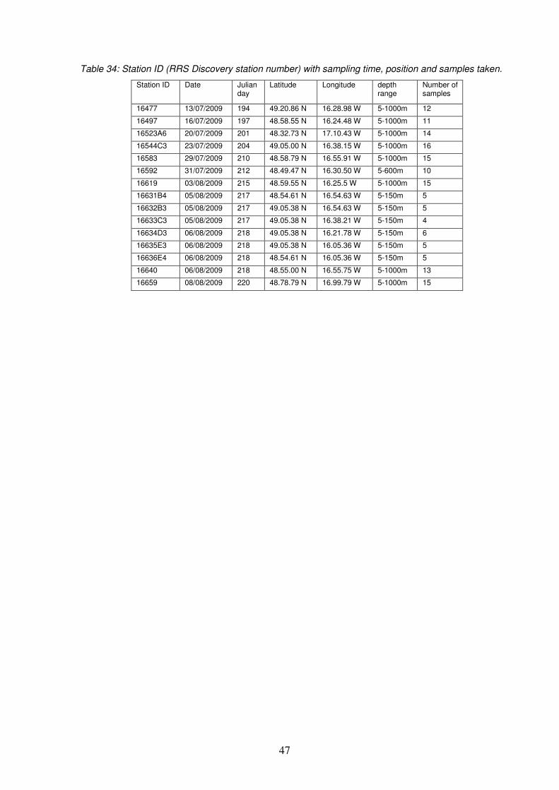
47
Table 34: Station ID (RRS Discovery station number) with sampling time, position and samples taken.
Station ID Date Julian day
Latitude Longitude depth range
Number of samples
16477 13/07/2009 194 49.20.86 N 16.28.98 W 5-1000m 12
16497 16/07/2009 197 48.58.55 N 16.24.48 W 5-1000m 11
16523A6 20/07/2009 201 48.32.73 N 17.10.43 W 5-1000m 14
16544C3 23/07/2009 204 49.05.00 N 16.38.15 W 5-1000m 16
16583 29/07/2009 210 48.58.79 N 16.55.91 W 5-1000m 15
16592 31/07/2009 212 48.49.47 N 16.30.50 W 5-600m 10
16619 03/08/2009 215 48.59.55 N 16.25.5 W 5-1000m 15
16631B4 05/08/2009 217 48.54.61 N 16.54.63 W 5-150m 5
16632B3 05/08/2009 217 49.05.38 N 16.54.63 W 5-150m 5
16633C3 05/08/2009 217 49.05.38 N 16.38.21 W 5-150m 4
16634D3 06/08/2009 218 49.05.38 N 16.21.78 W 5-150m 6
16635E3 06/08/2009 218 49.05.38 N 16.05.36 W 5-150m 5
16636E4 06/08/2009 218 48.54.61 N 16.05.36 W 5-150m 5
16640 06/08/2009 218 48.55.00 N 16.55.75 W 5-1000m 13
16659 08/08/2009 220 48.78.79 N 16.99.79 W 5-1000m 15
48
Ammonium and macronutrients Peter Statham and Richard Sanders (NOCS) The work of the Plymouth Marine Laboratory personnel (Ian Brown) on board focused on the cycling of a variety of N species in the upper water column using N-15 tracers. In order not to add an excess of the isotopically enriched substrate it is important to know ambient concentrations of N species including ammonia, and so this measurement was carried out onboard. The technique is based on the method of Holmes et al. (1999) in which ammonia reacts with OPA (orthophthalaldehyde) in a borate buffered solution in the presence of sulphite; the sulphite reduces interferences from amines. The fluorescent product was measured in a TD700 Turner fluorometer fitted with a near UV mercury vapour lamp, an interference excitation filter at 350nm and a 410-600 nm combination emission filter. The detailed protocol followed used slight modifications of the Holmes technique as recommended by Martin Johnson (UEA) and Stuart Painter (NOCS). The modified method used, 800 µL of the mixed reagent (made as in Holmes) per 10 mL of sample or standard, and after mixing the solution is allowed to stand for typically 3 hours at room temperature to allow the reaction to go to completion. Multiple blanks and standards as well as seawater fluorescence at the analytical wavelengths were determined. No detectable fluorescence above background was noted from the untreated seawaters and so no correction was applied. The detection limit of the method as used typically ranged from10-20 nM (3 sigma blank), and this was adequate for the sampled upper water column. All handling steps were done in a laminar flow hood fitted with an ammonia absorbing filter pack on the inlet which thus provided a low ammonia environment in which to work. Precision was improved by reusing the polystyrene diluvials in which the fluorescent product was formed. This infers there is a low level random contamination form the uncleaned diluvials. The calibration slope decreased gradually over he course of the cruise, and has been ascribed (S. Painter, pers comm.) to a gradual degradation of the OPA reagent. During the cruise 10 profiles were measured and concentrations ranged from about 300 nM to less than detection limits. Although there were significant variations between profiles and often profiles were not sampled at high resolution, a general trend of highest concentrations in the surface waters with a frequent maximum at the base of the mixed layer was evident. Below are two example profiles from the main biogeochemistry station, profiles 16475 (Fig 4a) before and 16497 (Fig 4b) after a strong storm event with associated vertical mixing of the water column, and reduction in the magnitude and broadening of the ammonia maximum.
Figure 4a. Ammonia profile 16475 before the first storm of the cruise
Ammonia vs depth 16475
0
20
40
60
80
100
120
140
160
180
200
0 50 100 150 200 250 300
Ammonia nM
Depth
Figure 4b. Ammonia profile after first storm event
16497
0
50
100
150
200
250
0 50 100 150 200
Ammonia (nM)
Depth
.
Figure 5 shows a detailed profile of ammonium structure in the upper water column, where the base of the mixed layer was at about 50m. An interpretation is the lowest ammonium in the mixed layer is just below the surface where productivity is expected to be highest and therefore any ammonium produced is rapidly taken up keeping concentrations low. Moving deeper into the water column, more detritus is accumulating and more recycling of ammonium occurs. This process seems to reach a maximum at the base of the mixed layer, in-line with other profiles where maxima occurred at a similar location. Below the mixed layer where the detritus is much less abundant, concentrations very rapidly fall to undetectable levels.
49
Figure 5. Final profile of the cruise, when precision issues were better under control
16635
0
20
40
60
80
100
120
0 20 40 60 80 100 120 140 160 180
Ammonium (nM)
Depth
DL
. Reference: Holmes R.M., Aminot A., Kerouel R., Hooker B.A., and Peterson B.J. (1999) Can. J. Fish. Aquat. Sci. 56, 1801-1808. Macronutrients Samples for the analysis of nitrate, phosphate and silicate concentrations were drawn from Niskin bottles on all CTD casts, stored at 4C and analysed within 24hrs of collection. Due to a shortage of manpower on the cruise the final numbers were not worked up on board – this should take place in June 2010.
50
D341 Doms Recovery Terry Edwards (NOCS) The DOMS mooring was recovered on July 20th, the notes below were written following recovery to guide discussion over a possible redeployment. In the event no redeployment was undertaken. The idea was to approach the surface buoy from upwind to inspect and assess the best options. This took into account the relative position of the buoy and anchor. The sighting pass confirmed damage to the buoy and put the lifting bale at around level with the stb deck. The idea was then to hook a 5T hook attached to the 3T deck winch cable directly into the bale and recover using the stb crane and ships wide block. The hook missed the top bale and became snagged on the ARGOS beacon brackets. It was then decided to hook the recover line so the 5T hook could be freed while keeping the buoy captive. The recovery line was eventually used to lift the buoy on board. The chain was then stopped off. This proved quite difficult as using the stb crane to recover the buoy meant the tugger, stopper and buoy were all in the same line. We attempted to leave the chain connected to the buoy while the chain was tugged / stopped / tugged. However, it was noticed that the chain / buoy connection shackle was almost out so we reverted to the plan of mechanically and electrically disconnecting the chain and buoy. After this, it was relatively easy to pull the chain up with the 3T winch. The first tugged length took the chain, wires and clamps through the block which didn’t work well as the clamps snagged the block and it jumped heavily when it released. The procedure then changed to hauling the cable through the block until the chain reached the block then stop off. This worked well. Frame came to the surface and was lifted out on stb crane. Swung forward and laid down on pallets. This was a bit awkward. But not too difficult. The wire was stopped off with 2 carpenters stops. This worked well, and the tail rope was connected through the DB winch. The rope was tied through the encapsulated wire swage as it was too wide for a shackle. This arrangement destroyed the encapsulation but was otherwise effective. The ship steamed to 0.5kts away from the anchor location as the wire was hauled in. The aim was to fire the release at 1.8NM from the anchor. Monitoring of the wire showed high tension so the release was fired at 1.7NM. 1127 GMT. The release was tracked until happy that it was ascending. The procedure worked fairly well, the line came to the surface untangled. After this, the recovery went as normal with only minor hitches when the drive arm on the drum reeler bent and had to be reinforced. Recommendations. Have wire from 3T winch go through the scrolling 3T winch should be more central Grab recovery line on stb side to help get the hook in the lifting bale. Disconnect chain from buoy immediately. Preliminary Report The section below is a copy of the preliminary report produced to focus attention on the 3 main issues that could prevent redeployment. This report will concentrate only on the issues that will directly or seriously affect redeployment of the mooring and look at actions required and by whom. There are more minor issues, but not show stoppers.
51
It is well worth noting that the major problems are all at the top end, the frame, wire, rope and lower buoyancy are all in very good condition and no modifications are necessary. The rest of the buoy, wiring, radar reflector etc is all in A1 condition. If we can deploy until AMT then a top buoy refurbishment / repair / replacement should be possible, as a full recovery will not be necessary. Loss of solar panels. The loss of 3 solar panels and their mountings appears to be a function of the buoy design that allows water to flush through. Regardless, what we have now is one large panel and 3 old small units, 2 of which were intended for use with AIS.
The question is, would a combination of these allow a reduced instrument and comms capability, and if so, what is the best option? This should be considered with the fact that we now have a stand alone iridium beacon to fit to the unit, so position monitoring is not an issue.
Bear in mind also that only the microcats have inductive couplers now, so if no hub, then only CTD data can be real time. Note that the hub has begun to corrode quite badly, it may be necessary to coat it somehow.
Action Jon and Richard to consult Buoy / Chain Junction The shackle and bush arrangement is clearly not substantial enough or does not have the right characteristics for this type of installation. Strangely, this type of wear was not an issue on the 2007 deployment. It could be a function of the extra weight or drag of the larger instrument frame. This is potentially a show stopper unless a new system can be devised.
Below is a picture of the worn shackle and pin. (Figure 6)
Figure 6. Photograph showing erosion of threads in main shackle holding instrument frame to buoy
So, how to attach a length of galvanized steel chain to a stainless steel eye in such a way that wear is reduced and movement is restricted?
Action: Terry, Kevin , Sam and Darren to address this on ship any suggestions from anybody will be considered.
We already have some ideas and will send them back as they shape up.
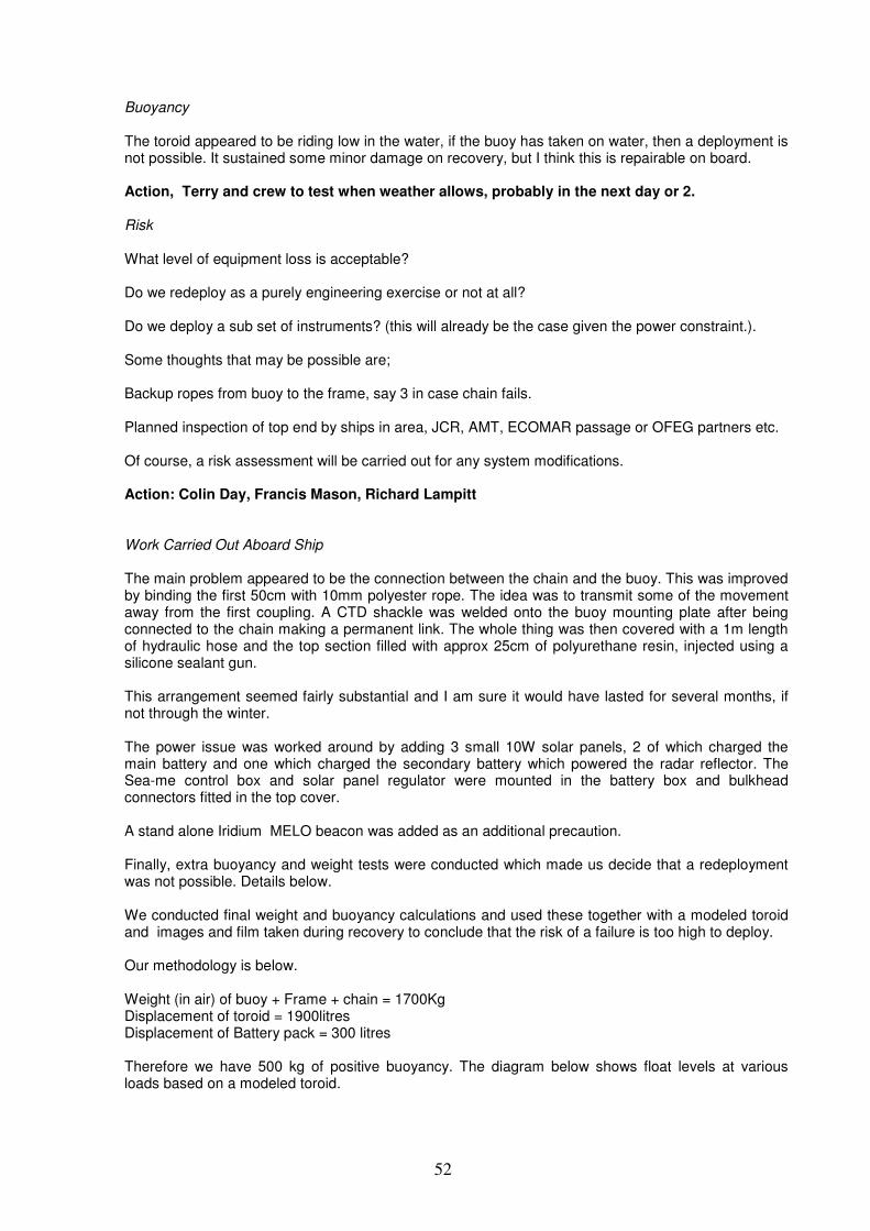
52
Buoyancy The toroid appeared to be riding low in the water, if the buoy has taken on water, then a deployment is not possible. It sustained some minor damage on recovery, but I think this is repairable on board.
Action, Terry and crew to test when weather allows, probably in the next day or 2.
Risk What level of equipment loss is acceptable?
Do we redeploy as a purely engineering exercise or not at all?
Do we deploy a sub set of instruments? (this will already be the case given the power constraint.).
Some thoughts that may be possible are;
Backup ropes from buoy to the frame, say 3 in case chain fails.
Planned inspection of top end by ships in area, JCR, AMT, ECOMAR passage or OFEG partners etc.
Of course, a risk assessment will be carried out for any system modifications.
Action: Colin Day, Francis Mason, Richard Lampitt Work Carried Out Aboard Ship The main problem appeared to be the connection between the chain and the buoy. This was improved by binding the first 50cm with 10mm polyester rope. The idea was to transmit some of the movement away from the first coupling. A CTD shackle was welded onto the buoy mounting plate after being connected to the chain making a permanent link. The whole thing was then covered with a 1m length of hydraulic hose and the top section filled with approx 25cm of polyurethane resin, injected using a silicone sealant gun. This arrangement seemed fairly substantial and I am sure it would have lasted for several months, if not through the winter. The power issue was worked around by adding 3 small 10W solar panels, 2 of which charged the main battery and one which charged the secondary battery which powered the radar reflector. The Sea-me control box and solar panel regulator were mounted in the battery box and bulkhead connectors fitted in the top cover. A stand alone Iridium MELO beacon was added as an additional precaution. Finally, extra buoyancy and weight tests were conducted which made us decide that a redeployment was not possible. Details below. We conducted final weight and buoyancy calculations and used these together with a modeled toroid and images and film taken during recovery to conclude that the risk of a failure is too high to deploy. Our methodology is below. Weight (in air) of buoy + Frame + chain = 1700Kg Displacement of toroid = 1900litres Displacement of Battery pack = 300 litres Therefore we have 500 kg of positive buoyancy. The diagram below shows float levels at various loads based on a modeled toroid.
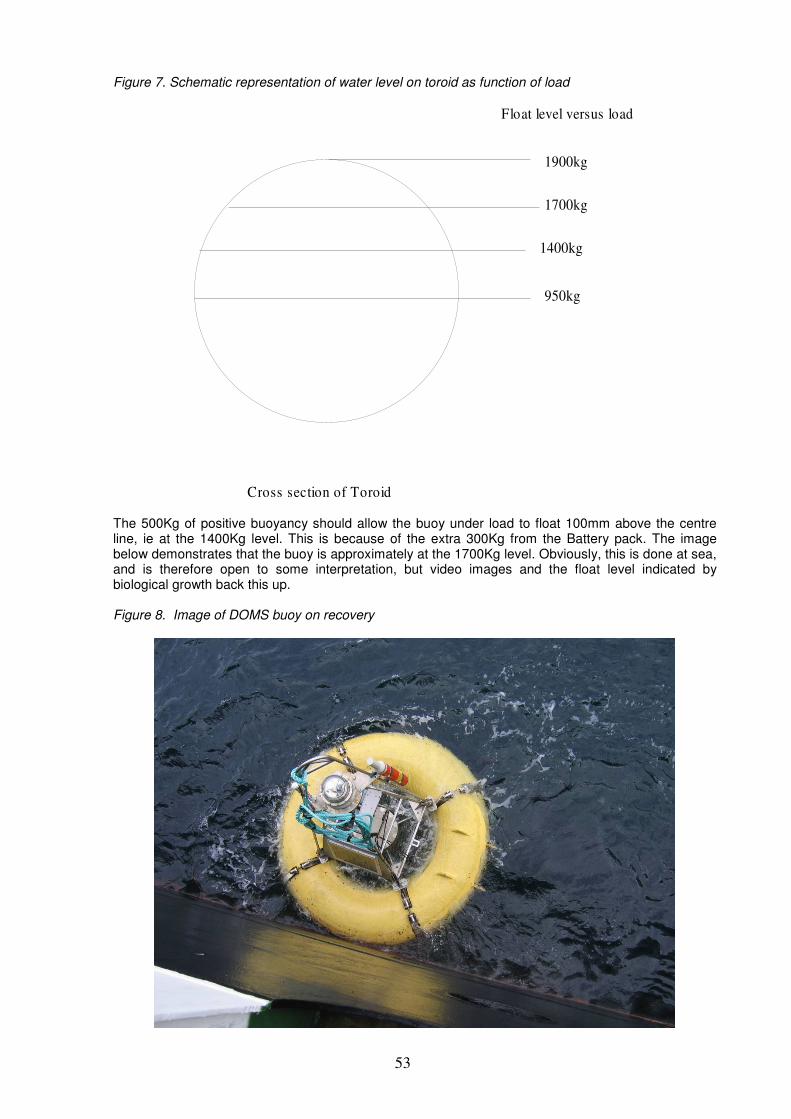
53
Figure 7. Schematic representation of water level on toroid as function of load
950kg
1400kg
1700kg
1900kg
Cross section of Toroid
Float level versus load
The 500Kg of positive buoyancy should allow the buoy under load to float 100mm above the centre line, ie at the 1400Kg level. This is because of the extra 300Kg from the Battery pack. The image below demonstrates that the buoy is approximately at the 1700Kg level. Obviously, this is done at sea, and is therefore open to some interpretation, but video images and the float level indicated by biological growth back this up. Figure 8. Image of DOMS buoy on recovery

54
This all means that we have around about 10% backup buoyancy available instead of a theoretical 20-25%. It does point to water ingress of the buoy, and this may be investigated at a future point, but we do not consider 10% adequate to risk a deployment of such a large installation in such a harsh environment. Additional buoyancy added at the last deployment was dislodged and we do not have the resources on board to confidently add buoyancy to any element of the mooring.
55
Microbial community abundance, structure and dynamics Mike Zubkov, Ross Holland (NOCS) The aim: To study abundance, community composition and metabolic activities of dominant microbial groups within planktonic communities of the twilight zone and to assess the rates of their nutrient acquisition and metabolism. Objectives: 1) To determine the spatial distribution, abundance and community structure of nano- and
picoplankton in the twilight zone by flow cytometry. 2) To collect concentrated seawater samples for analysis of plankton community composition in the
twilight zone using molecular approaches. 3) To estimate the turnover of dissolved organic nutrients and phosphorus using methionine, leucine
and ATP tracers. 4) To determine composition and abundance of microplankton down to the twilight zone. 2. Plankton community structure and abundance by flow cytometry. Seawater samples for flow cytometric analyses were collected from CTD bottles at stations and depths (Table 35) and 3.5 ml from each bottle sample were fixed with paraformaldehyde (PFA, final concentration 1%). Samples of 3.5 ml were left unfixed and unstained and were analysed live by flow cytometry within an hour of collection. Samples were analysed on a Becton Dickinson FACSCalibur (BD Biosciences, Oxford, UK) Analytical Flow Cytometer. Samples were analysed live unstained as well as fixed stained with SYBR Green I DNA stain. Three analysis protocols were used to resolve and enumerate populations of heterotrophic prokaryotes, picoplanktonic and nanoplanktonic algae and heterotrophic protists on bivariate dotplots of 90
o light scatter and green (DNA stain) fluorescence,
orange fluorescence and red fluorescence. Protocol 1 was used to analyse heterotrophic prokaryotes including cyanobacteria abundance
and distribution in the stained sample on bivariate dotplots of 90o light scatter (cell size index), red
fluorescence (chlorophyll content) and orange fluorescence (phycoerythrin content) against green fluorescence (DNA content). Protocol 3 was used to analyse heterotrophic protists, picophytoplankton and nanophytoplankton groups in the stained sample on bivariate dotplots of red fluorescence and orange fluorescence against green fluorescence. Protocol 2 was used on the unstained sample to confirm or deny the assumption that autofluorescent cells can be as effectively enumerated using DNA stained samples as with unstained samples, without a loss of pigment leading to undercounting. Protocol 1 was used to analyse all samples except those from CTD 16488. Protocol 2 was used to analyse all samples without exception. Protocol 3 was used to analyse all samples except those from CTDs 16475 and 16488. A total of fourteen CTD profiles were analysed by flow cytometry as outlined below in Table 35, in addition bacterioplankton was enumerated in samples of interest to other cruise participants.
Table 35. Table of bacterioplankton samples taken during cruise D341.
Discovery Station Number
D341 cruise Number
Date Time, GMT Bottle Number
Depth, m
16475 1 13/07/2009 05:21 1 4800
4 2000
6 1500
8 1000
10 750
12 500
14 300
16 200
18 100
20 80
21 60
22 40
23 20
24 10
16488 4 15/07/2009 00:55 1 800
56
2 800
3 800
4 800
5 800
6 800
7 800
8 800
16496 5 16/07/2009 1 1000
3 750
7 500*
9 300
11 200
13 150
15 100
17 80
19 50
21 25
23 5*
SWAB.1 18/07/2009 13:30 1*
16510 7 19/07/2009 04:48 3 1000*
4 900
5 750
6 600
7 500*
8 400
9 300
10 200
11 100
12 80
13 50
15 35
19 15
20 10
22 6
SWAB.2 20/07/2009 12:40 1*
16526 11 21/07/2009 08:21 1 1000
3 1000*
4 750
5 600
7 500*
8 300
9 150
10 100
11 75
12 50
13 25
14 5
16535 17 22/07/2009 05:43 2 1000*
4 750*
6 600
8 500*
10 300
12 150
14 100
16 75
18 50
20 25
24 5
16546 25 23/07/2009 11:02 2 1000
6 750*
10 500
12 300
14 150
16 100
18 75
20 50
57
22 25
24 5
16554 32 24/07/2009 06:30 2 1000
4 750
8 500*
10 300
12 150
14 75
16 50
18 25
24 5
16564 40 25/07/2009 2 1000
3 750
4 600
6 500
9 300*
10 150
12 100
14 75
16 50
19 25
24 5
SWAB.3 26/07/2009 13:10 1*
16583 45 29/07/2009 06:17 1 1000*
3 900
4 800
5 750
6 700
7 650
8 600
9 550
10 500
11 450
12 400
13 350
14 300
15 250
16 200
17 150
19 125
20 100
21 75
22 50
23 25
24 5
16592 47 31/07/2009 11:52 1 2000
3 600
4 500
5 400
6 200
7 150
8 125
9 100
11 75
13 50
15 25
17 5
16604 49 01/08/2009 07:25 2 1000
4 750
7 500*
9 300
11 150
13 100
14 75
16 50
20 25
58
24 5
SWAB.4 02/08/2009 14:59 1*
16619 54 03/08/2009 1 1000
2 800
5 750*
6 600
7 500
8 400
9 300
10 250
11 200
12 150
14 100
15 80
16 60
18 50
20 40
21 25
23 5
16636 64 06/08/2009 05:00 1 1000
3 750
5 600
7 500
11 300*
12 150
14 100
16 75
19 50
21 25
23 5
16659 70 08/08/2009 10:08 1 1000
3 875*
4 800
5 700
6 600
7 500
9 400
10 250
11 150
12 100
13 80
14 60
15 50
16 40
18 25
22 5
2. Microbial cell collection for molecular analyses of phylogenetic composition of planktonic microbial communities. Seawater samples of 10-20L were collected from CTD bottles (Table 35, asterisks) and after prefiltration through 20µm to screen out larger organisms microbial cells were concentrated. The concentrates were frozen in liquid nitrogen and stored at -80°C for further analyses ashore. 3. Assessment of metabolic activities of dominant planktonic microbes in twilight zone. Seawater samples of 20L were collected from CTD bottles (Table 35, asterisks) and ambient concentrations and turnover rates of two amino acids, leucine and methionine, and ATP by total bacterioplankton were measured using isotopic dilution time-series bioassays. On four occasions (Table 35) samples were collected using a surface water acquisition bucket (SWAB) and used for bioassays to compare with microbial metabolic rates in the twilight zone. The samples collected were used for bioassay incubations within <1/2 hour of collection.

59
4. PROgrammable Ocean Fractionation Net (PROOFNet) / FLOWCAM Trials. A novel method of collecting and size fractionating microplankton over a user-defined depth was trailed on D341. The Programmable Ocean Fractionation Net (PROOFNet) has a nested series of meshes of decreasing pore size, (180, 100, and 40µm) each with its own collection cod-end (Figures 9+10). The opening and closure of the meshes is controlled using a depth programmable operculum system. This enables the net to be opened and closed over a user-specified depth-range. Associated with the PROOFNet is a Nobska Velocity Meter which logs the inflow of water through the operculum in order to calculate the abundance and distribution of diverse microplankton groups over a specific depth range in the water column. The trials were conducted as detailed below in Table 36. Figures 9+10. PROOFNet being deployed
. Table 36. Deployments of PROOFnet
Cast Date Cast Time Depth Range Technical Notes
14/07/2009 12:00 90m - 40m Operculum function normal. No flow data recovered. User error.
15/07/2009 08:00 90m - 40m Operculum function normal. No flow data recovered. User error.
17/09/2009 08:30 90m - 40m Operculum opened. Flow data recovered. Unusual flow signal
recorded after closure, electronic error suspected.
19/07/2009 07:20 90 - 40m Operculum opened. Flow data recovered. Unusual flow signal
recorded after closure, electronic error confirmed.
As the error occurs after operculum re-closure, flow data during
open period assumed to be correct.
21/07/2009 16:42 90m - surface Operculum opened. Cast used as a control to confirm that
closure on previous casts was effective.
22/07/2009 15:26 90m - 40m Operculum Opened. Flow data recovered.
24/07/2009 16:15 90m - 40m To minimise observed outflow of water (Possibly due to ship roll)
from net, a faster net recovery was trialed (>10m/min).
Operculum opened, but failed to close properly. After this
deployment, velocity meter suffered electronic malfunction
and was deemed irreparable on the ship.
06/08/2009 20:00 100m - Surface Net deployed without opening and closing mechanism.
07/08/2009 20:00 100m - Surface Net deployed without opening and closing mechanism.
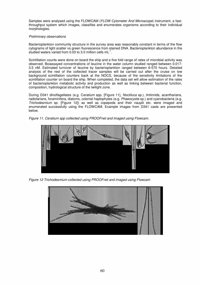
60
Samples were analysed using the FLOWCAM (FLOW Cytometer And Microscope) instrument, a fast-throughput system which images, classifies and enumerates organisms according to their individual morphologies. Preliminary observations Bacterioplankton community structure in the survey area was reasonably constant in terms of the flow cytograms of light scatter vs green fluorescence from stained DNA. Bacterioplankton abundance in the studied waters varied from 0.03 to 3.0 million cells mL
-1.
Scintillation counts were done on board the ship and a five fold range of rates of microbial activity was observed. Boiassayed concentrations of leucine in the water column studied ranged between 0.017-3.5 nM. Estimated turnover of leucine by bacterioplankton ranged between 6-570 hours. Detailed analysis of the rest of the collected tracer samples will be carried out after the cruise on low background scintillation counters back at the NOCS, because of the sensitivity limitations of the scintillation counter on board the ship. When completed, the data set will allow estimation of the rates of bacterioplankton metabolic activity and production as well as linking between bacterial function, composition, hydrological structure of the twilight zone. During D341 dinoflagellates (e.g. Ceratium spp. [Figure 11], Noctiluca sp.), tintinnids, acantharians, radiolarians, foraminifera, diatoms, colonial haptophytes (e.g. Phaeocystis sp.) and cyanobacteria (e.g. Trichodesmium sp. [Figure 12]) as well as copepods and their nauplii etc. were imaged and enumerated successfully using the FLOWCAM. Example images from D341 casts are presented below. Figure 11. Ceratium spp collected using PROOFnet and imaged using Flowcam.
Figure 12 Trichodesmium collected using PROOFnet and imaged using Flowcam
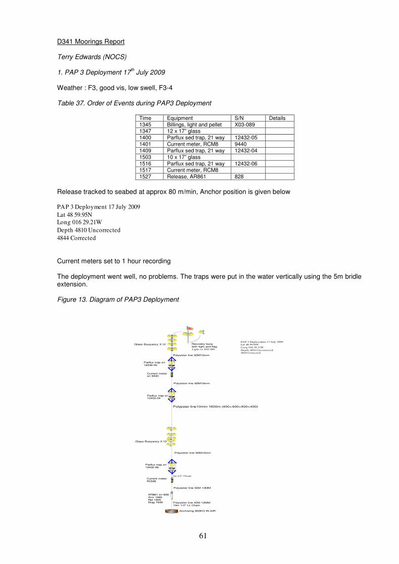
61
D341 Moorings Report Terry Edwards (NOCS) 1. PAP 3 Deployment 17
th July 2009
Weather : F3, good vis, low swell, F3-4 Table 37. Order of Events during PAP3 Deployment
Time Equipment S/N Details 1345 Billings, light and pellet X03-089 1347 12 x 17” glass 1400 Parflux sed trap, 21 way 12432-05 1401 Current meter, RCM8 9440 1409 Parflux sed trap, 21 way 12432-04 1503 10 x 17” glass 1516 Parflux sed trap, 21 way 12432-06 1517 Current meter, RCM8 1527 Release, AR861 828
Release tracked to seabed at approx 80 m/min, Anchor position is given below PAP 3 Deployment 17 July 2009
Lat 48 59.95N
Long 016 29.21W
Depth 4810 Uncorrected
4844 Corrected Current meters set to 1 hour recording The deployment went well, no problems. The traps were put in the water vertically using the 5m bridle extension. Figure 13. Diagram of PAP3 Deployment
Glass Buoyancy X 12
Current meterRCM8
Parflux trap sn12432-05
Polyester line10mm 1600m (400+400+400+400)
Glass Buoyancy X 10
Parflux trap sn 12432-04
Polyester line 45M 12MM10m 1/2" LL Chain
AR861 sn 828Arm 1665Rel 1655Diag 1649
Anchoring 850KG IN AIR
Recovery buoywith light and flag
Polyester line 50M10mm
Light sn X03-089
Polyester line 50M 10MM
1m 1/2" Chain
Current metersn 9440
Polyester line 50M10mm
PAP 3 Deployment 17 July 2009
Lat 48 59.95N
Long 016 29.21W
Depth 4810 Uncorrected
4844 Corrected
Polyester line 50M10mm
Parflux trap sn 12432-06
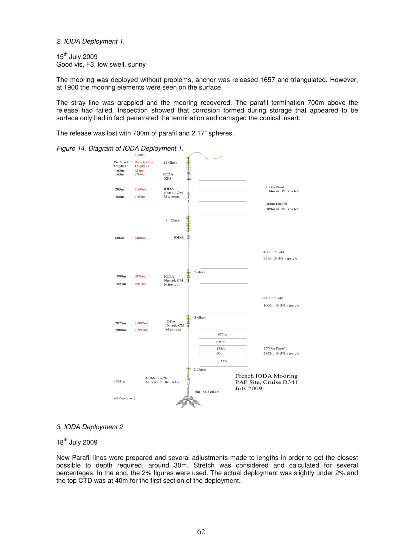
62
2. IODA Deployment 1. 15
th July 2009
Good vis, F3, low swell, sunny The mooring was deployed without problems, anchor was released 1657 and triangulated. However, at 1900 the mooring elements were seen on the surface. The stray line was grappled and the mooring recovered. The parafil termination 700m above the release had failed. Inspection showed that corrosion formed during storage that appeared to be surface only had in fact penetrated the termination and damaged the conical insert. The release was lost with 700m of parafil and 2 17” spheres. Figure 14. Diagram of IODA Deployment 1.
2750m Parafil
980m Parafil
480m Parafil
AR661 sn 261
Arm A171, Rel A172
300m Parafil
130m Parafil
IODA
Nortek CM
Microcat
IODA
Nortek CM
Microcat
IODA
Nortek CM
Microcat
IODA
IODA
12 Glass
14 Glass
3 Glass
3 Glass
2 Glass
5m 1/2 2 chain
ZPS
50m
700m
175m
975m
850m
4836m (corr)
4831m
2080m
2075m
1093m
1088m
606m
300m
295m
165m
163m
2832m @ 3% stretch
1009m @ 3% stretch
494m @ 3% stretch
309m @ 3% stretch
134m @ 3% stretch
Pre Stretch
Depths
(Stretched
Depths)
(1997m)
(1992m)
(981m)
(976m)
(480m)
(165m)
(160m)
(26m)(24m)
(18m)
French IODA Mooring
PAP Site, Cruise D341
July 2009
3. IODA Deployment 2 18
th July 2009
New Parafil lines were prepared and several adjustments made to lengths in order to get the closest possible to depth required, around 30m. Stretch was considered and calculated for several percentages. In the end, the 2% figures were used. The actual deployment was slightly under 2% and the top CTD was at 40m for the first section of the deployment.
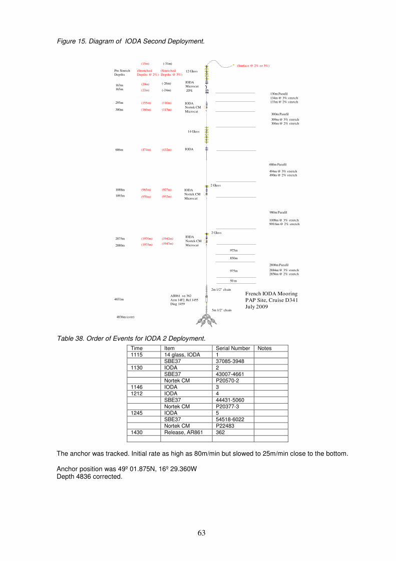
63
Figure 15. Diagram of IODA Second Deployment.
2800m Parafil
2884m @ 3% stretch
2856m @ 2% stretch
980m Parafil
1009m @ 3% stretch
999.6m @ 2% stretch
480m Parafil
494m @ 3% stretch
490m @ 2% stretch
AR861 sn 362
Arm 14F2, Rel 1455
Diag 1459
300m Parafil
309m @ 3% stretch
306m @ 2% stretch
130m Parafil
134m @ 3% stretch
133m @ 2% stretch
IODA
Nortek CM
Microcat
IODA
Nortek CM
Microcat
IODA
Nortek CM
Microcat
IODA
IODA
Microcat
12 Glass
14 Glass
2 Glass
2 Glass
5m 1/2" chain
ZPS
975m
850m
4836m (corr)
4831m
2080m
2075m
1093m
1088m
606m
300m
295m
165m
163m
Pre Stretch
Depths
(Stretched
Depths @ 3%)
(1947m)
(1942m)
(932m)
(927m)
(432m)
(115m)
(110m)
(-24m)
(-26m)
(-31m)
French IODA Mooring
PAP Site, Cruise D341
July 2009
975m
50 m
(1970m)
2m 1/2" chain
(1975m)
(970m)
(20m)
(22m)
(155m)
(160m)
(474m)
(965m)
(15m)
(Stretched
Depths @ 2%)
(Surface @ 2% or 3%)
Table 38. Order of Events for IODA 2 Deployment. The anchor was tracked. Initial rate as high as 80m/min but slowed to 25m/min close to the bottom. Anchor position was 49º 01.875N, 16º 29.360W Depth 4836 corrected.
Time Item Serial Number Notes 1115 14 glass, IODA 1 SBE37 37085-3948 1130 IODA 2 SBE37 43007-4661 Nortek CM P20570-2 1146 IODA 3 1212 IODA 4 SBE37 44431-5060 Nortek CM P20377-3 1245 IODA 5 SBE37 54518-6022 Nortek CM P22483 1430 Release, AR861 362
64
4. IODA Recovery 7
th July 2009
Wind F4, clear, vis good, bit of a swell Start time 0825 GMT The release was pinged from the ship standing approx 5 cables (1000m) downwind of anchor position. Initially, there were no comms and a decision was taken to fire. After a couple of attempts, a range of over 11000m was returned along with a release ok signal. This was initially taken as being a noise related spurious message. This was the only response received and after further attempts the ship repositioned and better ranges were obtained which confirmed the suspicion that the mooring had either been trawled or had dragged its anchor. The release was then triangulated and it became apparent that the release had actually fired at the initial communication. This was confirmed when 2 sets of range figures were received, one being a direct range and the other being a seabed reflection. The table below shows positions and ranges. Table 39. Ranges to anchor on IODA Recovery.
Time Lat N Long W Range Range Range Range Range 0837 49º 01.875 16º 29.360 11000 1015 49º 01.9 16º 29.3 10400 1055 48º 59.4 16º 31.9 9807 5965 9790 5952 5948 1135 48 º 47.86 16º 36.17 6041 9847 6005 9822 5975 1215 48 º 55.15 16º 34.07 4826 4822 4817
The glass packages were spotted on the surface at 48º 56.3N, 016º 32.6W. Recovery started at 1325 and was complete at 1645. 5. PAP 3 Recovery 29
th July 2009
Wind F5-6, clear, vis good, medium swell and choppy. The conditions were on the good side of marginal, but given the prevailing conditions it was considered a good idea to attempt retrieval. Table 40. Order of Events
Time Item Serial Number Notes 1458 Release fired 829 Good comms 1540 First glass sited 1555 Second glass sited 1610 Hooked stray line 1618 Billings on board 1627 Sed Trap on board 12168-01 1635 Sed Trap on board 11262-03 1700 Rope parted above second glass
package
1734 Glass hooked after vessel repositions
1746 Sed Trap on board 11262-02 1750 Release lost 829
The bottom section had become tangled and a large bight had formed. The rope appears to have chafed through in a couple of places resulting in the loss of the release.
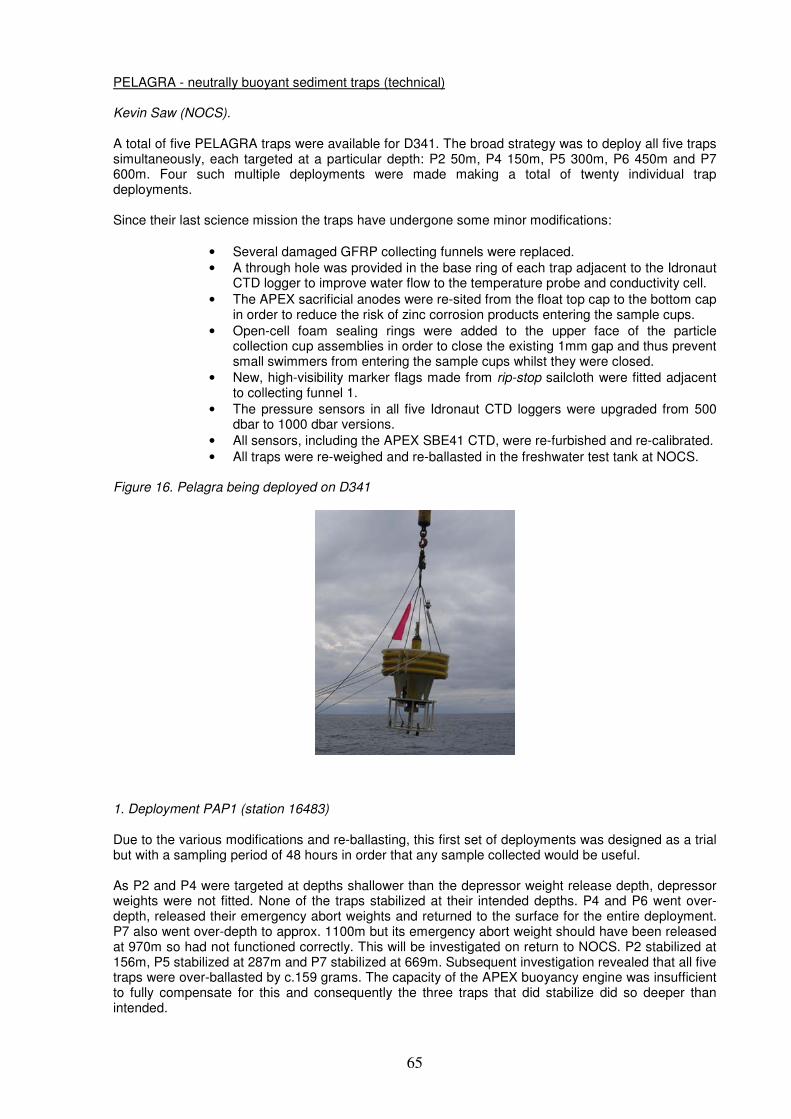
65
PELAGRA - neutrally buoyant sediment traps (technical) Kevin Saw (NOCS). A total of five PELAGRA traps were available for D341. The broad strategy was to deploy all five traps simultaneously, each targeted at a particular depth: P2 50m, P4 150m, P5 300m, P6 450m and P7 600m. Four such multiple deployments were made making a total of twenty individual trap deployments. Since their last science mission the traps have undergone some minor modifications:
• Several damaged GFRP collecting funnels were replaced. • A through hole was provided in the base ring of each trap adjacent to the Idronaut
CTD logger to improve water flow to the temperature probe and conductivity cell.
• The APEX sacrificial anodes were re-sited from the float top cap to the bottom cap in order to reduce the risk of zinc corrosion products entering the sample cups.
• Open-cell foam sealing rings were added to the upper face of the particle collection cup assemblies in order to close the existing 1mm gap and thus prevent small swimmers from entering the sample cups whilst they were closed.
• New, high-visibility marker flags made from rip-stop sailcloth were fitted adjacent to collecting funnel 1.
• The pressure sensors in all five Idronaut CTD loggers were upgraded from 500 dbar to 1000 dbar versions.
• All sensors, including the APEX SBE41 CTD, were re-furbished and re-calibrated.
• All traps were re-weighed and re-ballasted in the freshwater test tank at NOCS. Figure 16. Pelagra being deployed on D341
1. Deployment PAP1 (station 16483) Due to the various modifications and re-ballasting, this first set of deployments was designed as a trial but with a sampling period of 48 hours in order that any sample collected would be useful. As P2 and P4 were targeted at depths shallower than the depressor weight release depth, depressor weights were not fitted. None of the traps stabilized at their intended depths. P4 and P6 went over-depth, released their emergency abort weights and returned to the surface for the entire deployment. P7 also went over-depth to approx. 1100m but its emergency abort weight should have been released at 970m so had not functioned correctly. This will be investigated on return to NOCS. P2 stabilized at 156m, P5 stabilized at 287m and P7 stabilized at 669m. Subsequent investigation revealed that all five traps were over-ballasted by c.159 grams. The capacity of the APEX buoyancy engine was insufficient to fully compensate for this and consequently the three traps that did stabilize did so deeper than intended.
66
It should be noted that P2, P5 and P7 were not stable for the initial part of the sampling period. 2. Deployment PAP2 (stations 16515 - 16519) Deployment PAP2 was configured for a total sampling time of 132 hours. To compensate for the over-ballasting in deployment PAP1, the added ballast was reduced by 159 grams from that calculated by the ballast spreadsheets. As P2 and P4 were targeted at depths shallower than the depressor weight release depth, depressor weights were not fitted and both remained at the surface until the sample pots opened; this behaviour had not been observed before. It was postulated that the air-space at the top of each sample cup was prevented from venting by the new foam sealing rings and the additional buoyancy was sufficient to prevent the traps from sinking (this is to be verified). Once the sample cups opened, the air was released and the traps sank. Because the APEX buoyancy engine had already begun to reduce, P2 descended initially to 305m but recovered to stabilize at an average depth of 52m. It should be noted that P2 was unstable for the first 15 hours of sampling. P4 initially descended to 730m at which point its emergency over-depth release was triggered and it returned to the surface for the remainder of the deployment. Any excess trapped air buoyancy in P5, P6 and P7 was overcome by the depressor weights and all three traps successfully stabilized close to their target depths: 312m, 449m and 565m respectively. On deployment, funnel 1 on P5 was found to be cracked in several places. It is not clear how or when this occurred. There is no recollection that it was cracked on recovery of PAP1 so it is possible that it was damaged whilst on deck between deployments. 3. Deployment PAP3 (stations 16574 - 16578) In order to overcome the trapped air problem, P2 and P4 were fitted with depressor weights this time. Additionally, funnels 3 and 4 on P2 were fitted with c.10mm square mesh baffle grids in order to reduce the ingress of jelly-fish which had heavily contaminated some previous samples. (These were fashioned from SAPS pre-filter grids). During deployments PAP3 and PAP4 sample cups 3 and 4 remained free from jelly-fish whilst sample cups 1 and 2 did not, so the grids appear to be effective and should be considered as a permanent modification. Shortly after deployment it was discovered that an error had been made when compensating for the three less dense polypropylene sample cups that had replaced the standard polycarbonate cups. The error amounted to an under-ballast of c. 26 grams for P2 and c.214 grams for P4, P5, P6 and P7. Whilst this was insignificant for P2, it was felt that the other traps would not be able to achieve their target depths. P2 did in fact stabilize at an average depth of 49m as planned. Despite initially descending to 730m, P4 returned to the surface until the APEX buoyancy engine had reduced its volume to a minimum and stabilized at an average depth of 222m. It should be noted that P4 was unstable for the first 27 hours of sampling. P5 descended to 208m where the depressor weight was released but thereafter behaved similarly to P4, only despite the APEX buoyancy engine reducing to minimum volume the trap remained at the surface. It is suspected that this was exacerbated by trapped air in the sample cups which was released when the sample cups opened. At this point the trap sank rapidly (approx. 3hrs) and stabilized at an average depth of 48m. P6 behaved similarly to P4 only this time the combination of buoyancy engine reduction and released air was insufficient to sink the trap and it remained at or near the surface for more than half of its deployment. It did eventually stabilize at around 50m but it is unlikely that this trap will yield any useful sample. P7 also returned to the surface after releasing its depressor weight at 218m. Rapid descent occurred once the sample cups opened and the trap stabilized at an average depth of 205m. It should be noted that P7 was unstable for the first 14 hours of sampling.
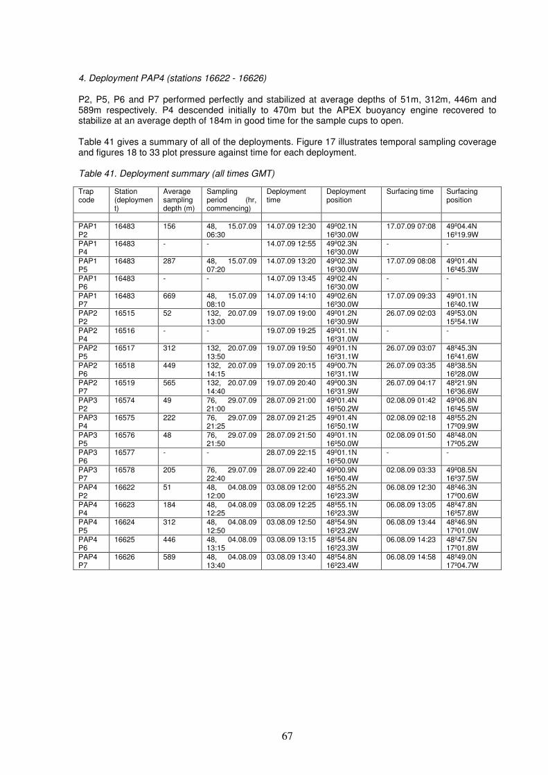
67
4. Deployment PAP4 (stations 16622 - 16626) P2, P5, P6 and P7 performed perfectly and stabilized at average depths of 51m, 312m, 446m and 589m respectively. P4 descended initially to 470m but the APEX buoyancy engine recovered to stabilize at an average depth of 184m in good time for the sample cups to open. Table 41 gives a summary of all of the deployments. Figure 17 illustrates temporal sampling coverage and figures 18 to 33 plot pressure against time for each deployment. Table 41. Deployment summary (all times GMT)
Trap code
Station (deployment)
Average sampling depth (m)
Sampling period (hr, commencing)
Deployment time
Deployment position
Surfacing time Surfacing position
PAP1 P2
16483 156 48, 15.07.09 06:30
14.07.09 12:30 49º02.1N 16º30.0W
17.07.09 07:08 49º04.4N 16º19.9W
PAP1 P4
16483 - - 14.07.09 12:55 49º02.3N 16º30.0W
- -
PAP1 P5
16483 287 48, 15.07.09 07:20
14.07.09 13:20 49º02.3N 16º30.0W
17.07.09 08:08 49º01.4N 16º45.3W
PAP1 P6
16483 - - 14.07.09 13:45 49º02.4N 16º30.0W
- -
PAP1 P7
16483 669 48, 15.07.09 08:10
14.07.09 14:10 49º02.6N 16º30.0W
17.07.09 09:33 49º01.1N 16º40.1W
PAP2 P2
16515 52 132, 20.07.09 13:00
19.07.09 19:00 49º01.2N 16º30.9W
26.07.09 02:03 49º53.0N 15º54.1W
PAP2 P4
16516 - - 19.07.09 19:25 49º01.1N 16º31.0W
- -
PAP2 P5
16517 312 132, 20.07.09 13:50
19.07.09 19:50 49º01.1N 16º31.1W
26.07.09 03:07 48º45.3N 16º41.6W
PAP2 P6
16518 449 132, 20.07.09 14:15
19.07.09 20:15 49º00.7N 16º31.1W
26.07.09 03:35 48º38.5N 16º28.0W
PAP2 P7
16519 565 132, 20.07.09 14:40
19.07.09 20:40 49º00.3N 16º31.9W
26.07.09 04:17 48º21.9N 16º36.6W
PAP3 P2
16574 49 76, 29.07.09 21:00
28.07.09 21:00 49º01.4N 16º50.2W
02.08.09 01:42 49º06.8N 16º45.5W
PAP3 P4
16575 222 76, 29.07.09 21:25
28.07.09 21:25 49º01.4N 16º50.1W
02.08.09 02:18 48º55.2N 17º09.9W
PAP3 P5
16576 48 76, 29.07.09 21:50
28.07.09 21:50 49º01.1N 16º50.0W
02.08.09 01:50 48º48.0N 17º05.2W
PAP3 P6
16577 - - 28.07.09 22:15 49º01.1N 16º50.0W
- -
PAP3 P7
16578 205 76, 29.07.09 22:40
28.07.09 22:40 49º00.9N 16º50.4W
02.08.09 03:33 49º08.5N 16º37.5W
PAP4 P2
16622 51 48, 04.08.09 12:00
03.08.09 12:00 48º55.2N 16º23.3W
06.08.09 12:30 48º46.3N 17º00.6W
PAP4 P4
16623 184 48, 04.08.09 12:25
03.08.09 12:25 48º55.1N 16º23.3W
06.08.09 13:05 48º47.8N 16º57.8W
PAP4 P5
16624 312 48, 04.08.09 12:50
03.08.09 12:50 48º54.9N 16º23.2W
06.08.09 13:44 48º46.9N 17º01.0W
PAP4 P6
16625 446 48, 04.08.09 13:15
03.08.09 13:15 48º54.8N 16º23.3W
06.08.09 14:23 48º47.5N 17º01.8W
PAP4 P7
16626 589 48, 04.08.09 13:40
03.08.09 13:40 48º54.8N 16º23.4W
06.08.09 14:58 48º49.0N 17º04.7W
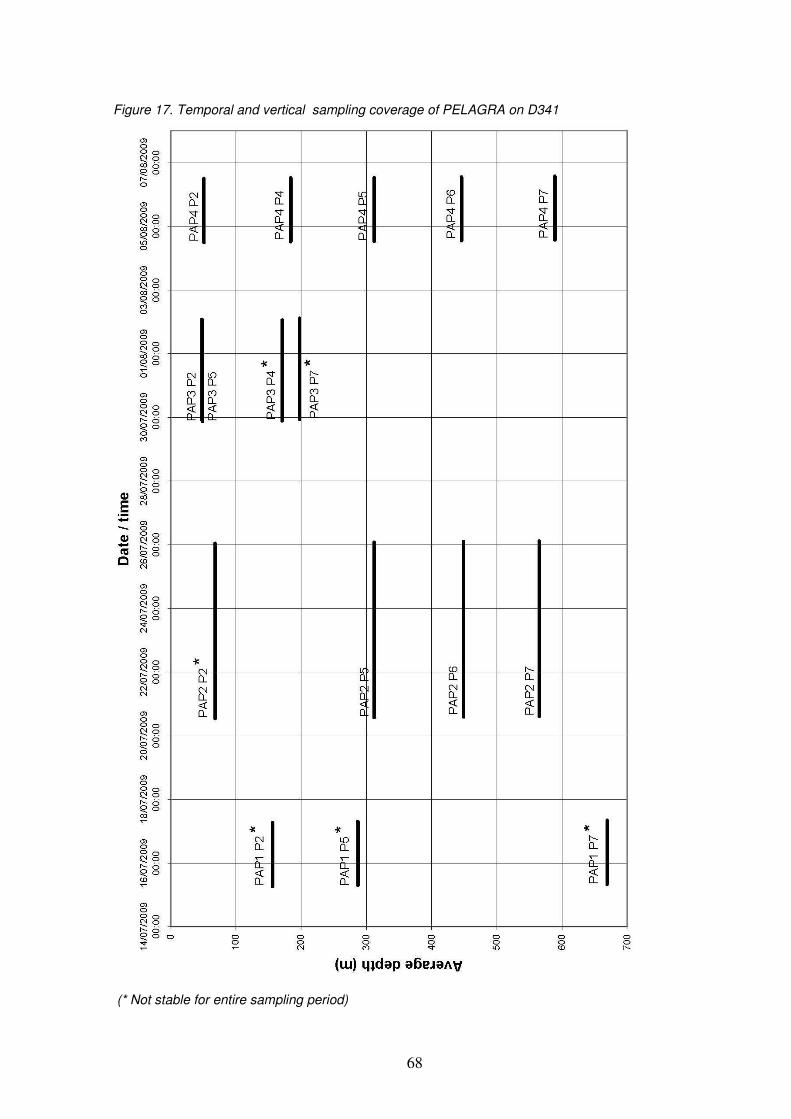
68
Figure 17. Temporal and vertical sampling coverage of PELAGRA on D341
(* Not stable for entire sampling period)

69
Figure 18. PAP1 P2, station 16483
Figure 19. PAP1 P5, station 16483
Figure 20. PAP1 P7, station 16483
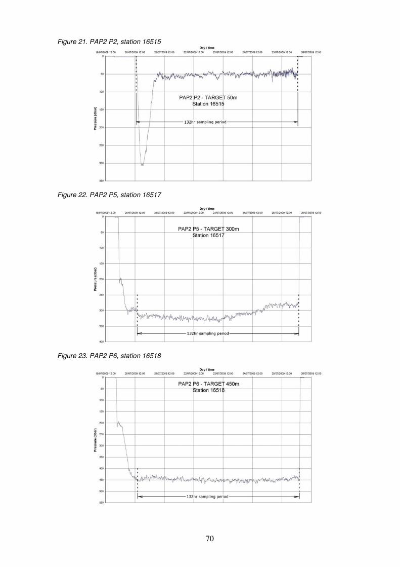
70
Figure 21. PAP2 P2, station 16515
Figure 22. PAP2 P5, station 16517
Figure 23. PAP2 P6, station 16518
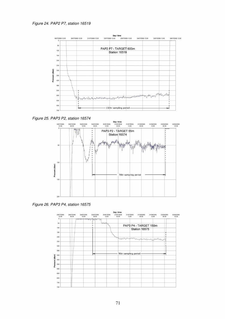
71
Figure 24. PAP2 P7, station 16519
Figure 25. PAP3 P2, station 16574
Figure 26. PAP3 P4, station 16575
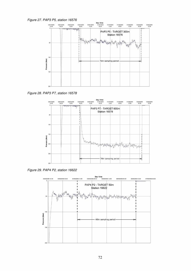
72
Figure 27. PAP3 P5, station 16576
Figure 28. PAP3 P7, station 16578
Figure 29. PAP4 P2, station 16622
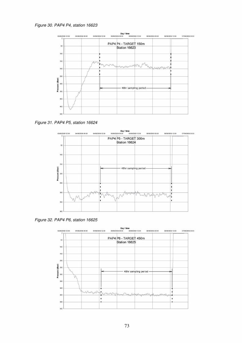
73
Figure 30. PAP4 P4, station 16623
Figure 31. PAP4 P5, station 16624
Figure 32. PAP4 P6, station 16625
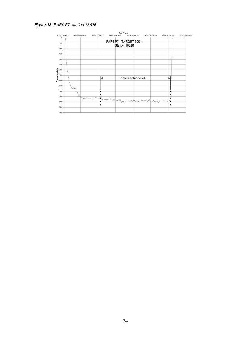
74
Figure 33. PAP4 P7, station 16626
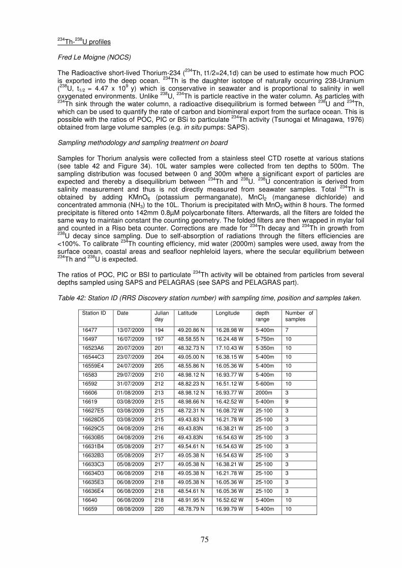
75
234Th-
238U profiles
Fred Le Moigne (NOCS) The Radioactive short-lived Thorium-234 (
234Th, t1/2=24,1d) can be used to estimate how much POC
is exported into the deep ocean. 234
Th is the daughter isotope of naturally occurring 238-Uranium (238
U, t1/2 = 4.47 x 10⁹
y) which is conservative in seawater and is proportional to salinity in well oxygenated environments. Unlike
238U,
234Th is particle reactive in the water column. As particles with
234Th sink through the water column, a radioactive disequilibrium is formed between
238U and
234Th,
which can be used to quantify the rate of carbon and biomineral export from the surface ocean. This is possible with the ratios of POC, PIC or BSi to particulate
234Th activity (Tsunogai et Minagawa, 1976)
obtained from large volume samples (e.g. in situ pumps: SAPS). Sampling methodology and sampling treatment on board Samples for Thorium analysis were collected from a stainless steel CTD rosette at various stations (see table 42 and Figure 34). 10L water samples were collected from ten depths to 500m. The sampling distribution was focused between 0 and 300m where a significant export of particles are expected and thereby a disequilibrium between
234Th and
238U.
238U concentration is derived from
salinity measurement and thus is not directly measured from seawater samples. Total 234
Th is obtained by adding KMnO6 (potassium permanganate), MnCl2 (manganese dichloride) and concentrated ammonia (NH3) to the 10L. Thorium is precipitated with MnO2 within 8 hours. The formed precipitate is filtered onto 142mm 0.8µM polycarbonate filters. Afterwards, all the filters are folded the same way to maintain constant the counting geometry. The folded filters are then wrapped in mylar foil and counted in a Riso beta counter. Corrections are made for
234Th decay and
234Th in growth from
238U decay since sampling. Due to self-absorption of radiations through the filters efficiencies are
<100%. To calibrate 234
Th counting efficiency, mid water (2000m) samples were used, away from the surface ocean, coastal areas and seafloor nephleloid layers, where the secular equilibrium between 234
Th and 238
U is expected. The ratios of POC, PIC or BSI to particulate
234Th activity will be obtained from particles from several
depths sampled using SAPS and PELAGRAS (see SAPS and PELAGRAS part). Table 42: Station ID (RRS Discovery station number) with sampling time, position and samples taken.
Station ID Date Julian day
Latitude Longitude depth range
Number of samples
16477 13/07/2009 194 49.20.86 N 16.28.98 W 5-400m 7
16497 16/07/2009 197 48.58.55 N 16.24.48 W 5-750m 10
16523A6 20/07/2009 201 48.32.73 N 17.10.43 W 5-350m 10
16544C3 23/07/2009 204 49.05.00 N 16.38.15 W 5-400m 10
16559E4 24/07/2009 205 48.55.86 N 16.05.36 W 5-400m 10
16583 29/07/2009 210 48.98.12 N 16.93.77 W 5-400m 10
16592 31/07/2009 212 48.82.23 N 16.51.12 W 5-600m 10
16606 01/08/2009 213 48.98.12 N 16.93.77 W 2000m 3
16619 03/08/2009 215 48.98.66 N 16.42.52 W 5-400m 9
16627E5 03/08/2009 215 48.72.31 N 16.08.72 W 25-100 3
16628D5 03/08/2009 215 49.43.83 N 16.21.78 W 25-100 3
16629C5 04/08/2009 216 49.43.83N 16.38.21 W 25-100 3
16630B5 04/08/2009 216 49.43.83N 16.54.63 W 25-100 3
16631B4 05/08/2009 217 49.54.61 N 16.54.63 W 25-100 3
16632B3 05/08/2009 217 49.05.38 N 16.54.63 W 25-100 3
16633C3 05/08/2009 217 49.05.38 N 16.38.21 W 25-100 3
16634D3 06/08/2009 218 49.05.38 N 16.21.78 W 25-100 3
16635E3 06/08/2009 218 49.05.38 N 16.05.36 W 25-100 3
16636E4 06/08/2009 218 48.54.61 N 16.05.36 W 25-100 3
16640 06/08/2009 218 48.91.95 N 16.52.62 W 5-400m 10
16659 08/08/2009 220 48.78.79 N 16.99.79 W 5-400m 10
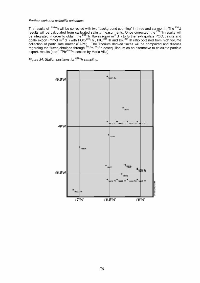
76
Further work and scientific outcomes The results of
234Th will be corrected with two “background counting” in three and six month. The
238U
results will be calculated from calibrated salinity measurments. Once corrected, the 234
Th results will be integrated in order to obtain the
234Th fluxes (dpm m
-2 d
-1) to further extrapolate POC, calcite and
opale export (mmol m-2
d-1
) with POC/234
Th , PIC/234
Th and Bsi/234
Th ratio obtained from high volume collection of particulate matter (SAPS). The Thorium derived fluxes will be compaired and discuss regarding the fluxes obtained through
210Pb-
210Po desequilibrium as an alternative to calculate particle
export. results (see 210
Pb/210
Po section by Maria Villa). Figure 34: Station positions for
234Th sampling.
77
Mid-water incubator Kevin Saw (NOCS) The mid-water incubator is a new instrument consisting of a rosette of 24 modified 20-litre Niskin bottles. Each Niskin bottle has been equipped with two fluid injection devices and an expansion bladder. Bottle firing and fluid injection is controlled by a purpose-built electronic timer system powered by one 24-volt Deep Sea Power and Light lead acid battery. The instrument is intended to be deployed on a long-term mooring to conduct in situ incubation experiments at depths of up to 6000m. It was hoped that the incubator would be deployed on a mooring on D341. However, administrative issues and late delivery of the instrument prevented this. Instead, D341 provided an opportunity to carry out trial deployments suspended from the ship’s CTD wire. On-deck tests of the electronic control system early in the cruise highlighted an issue that prevented the syringes on bottles 1 and 2 from firing. Whilst this issue was not wholly consistent, it did appear to affect only bottles 1 and 2. The decision was taken to go ahead with a shallow deployment whilst accepting that some syringes may not fire. In order to gain some insight into the effectiveness of fluid mixing within the closed bottles, the upper syringes were loaded with diluted blue food dye and the lower with yellow. A program was entered that would fire all 24 bottles and 48 syringes in the correct sequence at 1 minute intervals (5 minutes between bottle 1 and syringe 1) starting at 19:30 GMT. The incubator was deployed at 19:25 on 31 July 2009 from the CTD wire over the starboard gantry to a depth of 15m (station 16595). It was recovered to the deck at 21:10. On recovery it was noted that nothing had fired except that bottle 1 had closed (although the top bung was not seated properly). Subsequent investigations on deck yielded the same result: bottle 1 fired but nothing else. In fact the problem appeared to be related to the real-time clock in the controller as after bottle 1 had fired the next trigger time had been reset to a time prior to the current time and so was ignored by the program. Various updated versions of the controller firmware were supplied by colleagues at NOCS but none solved the problem. It was eventually concluded that the root of the problem most likely lay with the controller electronic hardware which is not repairable at sea; therefore no further sea-trials were conducted. Figure 35. Mid Water Incubator being deployed on D341
78
Organic Biogeochemistry Kostas Kiriakoulakis (University of Liverpool) 1. Particulate sampling (SAPS and PELAGRA traps): Organic chemical analyses Particulate material from a range of water depths was collected using stand alone pumping systems (SAPS; Challenger Oceanic, Table 43). Often two size fractions were recovered. The small fraction (>53 µm) was usually collected on large (293 mm diam.) precombusted (400ºC; 4 h) GF/F filters (nominal pore size 0.7 µm). Each SAPS carried two stacked GF/F filters, the bottom one being used as a DOM-adsorption blank. Occasionally small particles were collected on acid (10% HCL + 1% H2O2) cleaned Nylon mesh screens (pore size 1µm). Material was then rinsed with MilliQ water, filtered on a plastic rig through multiple precombusted (400ºC; 4 h) 25 mm GF/F filters and frozen at -80°C for the rest of the cruise. Larger particles were collected on acid (10% HCL + 1% H2O2) cleaned Nylon mesh screens (pore size 53 µm) that were positioned above the GF/F filters (or the smaller pore size Nylon screens). After recovery a similar procedure was carried out as for the smaller pore size Nylon screens (see above). Non size fractionated particulate material was also collected at certain deployments (Table 43) on large GF/F filters as described above. On recovery the filters and/or the rinsed material was split between partners for a range of chemical analyses, namely radionuclides (see reports by Maria Villa and Fred LeMoigne) and/or pigment analysis (Denise Smythe-Wright, NOCS). The part of the GF/F filters that was allocated for organic geochemical analyses (i.e. organic carbon, nitrogen, lipid biomarkers, stable isotopes) was frozen at -80°C for the duration of the cruise. Five or four SAPS units were used on the same deployment and the pumps were operated for 2 hours. Choice of depths was made to coincide with the depths of free-drifting (Pelagra) sediment traps when possible. These were usually 50, 150, 300, 450 and 600 m, although samples were also collected from the bottom of the twilight zone (1000 m) and in one deployment from 3000 and 4700 m (the latter two depths were chosen to coincide with the time series sediment traps that are moored in the PAP). Sinking particulate material from a range of water depths was also collected using five free drifting (Pelagra) sediment traps (Table 44). The preset depths were 50, 150, 300, 450 and 600 m although occasionally the traps malfunctioned and did not collect material from these depths (Table 44). Filtered, sterilised or deep (1000m) water with no preservative was used as a medium to collect the material, except the first deployment, when 0.5% CH3Cl was added in a concentrated brine solution that was used as a medium in that case (1/8 split with Chris Marsay). Occasionally large swimmers (jelly fish, shrimps etc.) were caught in the recipients. These were immediately removed on recovery and the sinking particles were filtered on a plastic rig through multiple precombusted (400ºC; 4 h) 25 mm GF/F filters and frozen at -80°C for the rest of the cruise. On return to the laboratory particulate material collected on the filters will be freeze-dried and analysed for organic carbon, nitrogen, lipids and isotopes (δ
13C and δ
15N).
Table 43. Details of SAPS sampling
Station Date SAPS depth
Volume pumped
Fractionated split
m L small fraction
large fraction
16498 16/07/2009 50 896 yes GF/F nylon 53 µm half
16498 16/07/2009 150 1462 yes GF/F nylon 53 µm half
16498 16/07/2009 150 2300 no GF/F half
16498 16/07/2009 600 623 yes GF/F nylon 53 µm half
16498 16/07/2009 600 1362 no GF/F half
16545 23/07/2009 50 2602 yes nylon 1µm nylon 53 µm quarter
16545 23/07/2009 150 2083 yes nylon 1µm nylon 53 µm quarter
79
Table 44. Details of Pelagra sampling
16545 23/07/2009 350 1070 no GF/F half
16545 23/07/2009 450 1326 yes GF/F (5.2g) nylon 53 µm half
16545 23/07/2009 600 1351 no GF/F half
16584 29/07/2009 50 1796 yes nylon 1µm nylon 53 µm quarter
16584 29/07/2009 150 973 yes nylon 1µm nylon 53 µm quarter
16587 29/07/2009 150 1402 yes GF/F nylon 53 µm half
16587 29/07/2009 300 449 yes GF/F nylon 53 µm half
16587 29/07/2009 450 1134 no GF/F half
16587 29/07/2009 600 1435 no GF/F half
16587 29/07/2009 1000 1251 yes GF/F (5.2g) nylon 53 µm half
16594 31/07/2009 60 920 yes nylon 1µm nylon 53 µm quarter
16594 31/07/2009 150 2164 yes nylon 1µm nylon 53 µm quarter
16598 01/08/2009 150 1466 yes GF/F nylon 53 µm half
16598 01/08/2009 300 1181 yes GF/F nylon 53 µm half
16598 01/08/2009 600 588 yes GF/F nylon 53 µm half
16598 01/08/2009 1000 1414 no GF/F half
16666 09/08/2009 150 1479 no GF/F half
16666 09/08/2009 600 589 no GF/F half
16666 09/08/2009 3000 1271 no GF/F half
16666 09/08/2009 4700 952 no GF/F half
Station Date Pelagra depth split medium preservative
deployment Deployment m
16483 14/07/2009 150 1/8. brine CH3Cl
16483 14/07/2009 300 1/8. brine CH3Cl
16483 14/07/2009 630 1/8. brine CH3Cl
16515 19/07/2009 50 half filtered seawater
no
16516 19/07/2009 150 did not work no filtered seawater
no
16517 19/07/2009 300 no filtered seawater
no
16518 19/07/2009 450 no filtered seawater
no
16519 19/07/2009 600 no filtered seawater
no
16574 28/07/2009 50 half sterilized water
no
16575 28/07/2009 150 (did not work)
no sterilized water
no
16576 28/07/2009 300 (50 actual) no deep water no
16577 28/07/2009 450 (did not work)
no deep water no
16578 28/07/2009 600 (200 actual) no deep water no
16622 03/08/2009 50 no deep water no
80
Two
sediment cores (deployments: 16499 and 16663; see report by Nina Rothe) were collected using the NOCS mega corer and were frozen upon recovery, extruded when still frozen, wrapped in pre-combusted (400ºC; 4 h) foil and stored in -80ºC for the duration of the cruise. On return to the laboratory the cores will be sectioned down to 10 cm, freeze-dried and analysed for organic carbon, nitrogen, lipids and isotopes (δ
13C and δ
15N).
2. Particulate sampling for pigment (HPLC) and microscopic analyses (for Denise Smythe-Wright) Particulate material for pigment analyses (HPLC) from a range of water depths was collected using a CTD rosette (Table 45). Two litres of water for each depth was filtered on a plastic rig through a 25 mm GF/F filter and frozen at -80°C for the rest of the cruise. Additionally 95ml of water from the same depths was spiked with 2 ml of LUGOL solution in dark bottles and kept at room temperature for phytoplankton identification. Table 45. Details of filtered material for pigment and microscopy (for Denise Smythe-Wright)
Station Date Depth CTD
CTD bottle
Filtering water (Lugol)
Lugol Bottle
m volume (L)
(ml) ml Lugol
16477 13/07/2009 400 6 2 95 2 A9
16477 13/07/2009 300 8 2 95 2 A8
16477 13/07/2009 200 10 2 95 2 A7
16477 13/07/2009 150 12 2 95 2 A6
16477 13/07/2009 100 14 2 95 2 A5
16477 13/07/2009 80 16 2 95 2 A4
16477 13/07/2009 50 18 2 95 2 A3
16477 13/07/2009 25 22 2 95 2 A2
16477 13/07/2009 5 24 2 95 2 A1
16497 16/07/2009 400 6 2 95 2 A18
16497 16/07/2009 300 10 2 95 2 A17
16497 16/07/2009 200 12 2 95 2 A16
16497 16/07/2009 150 14 2 95 2 A15
16497 16/07/2009 100 16 2 95 2 A14
16497 16/07/2009 80 18 2 95 2 A13
16497 16/07/2009 50 20 2 95 2 A12
16497 16/07/2009 25 22 2 95 2 A11
16497 16/07/2009 5 24 2 95 2 A10
16619 03/08/2009 5 24 2 95 2 A19
16619 03/08/2009 25 22 2 95 2 A20
16619 03/08/2009 50 20 2 95 2 A21
16619 03/08/2009 100 18 2 95 2 A22
16619 03/08/2009 150 16 2 95 2 A23
16619 03/08/2009 200 14 2 95 2 A24
16619 03/08/2009 300 12 2 95 2 A25
16619 03/08/2009 400 10 2 95 2 A26
16619 03/08/2009 600 6 2 95 2 A27
16623 03/08/2009 150 no deep water no
16624 03/08/2009 300 no deep water no
16625 03/08/2009 450 no deep water no
16626 03/08/2009 600 no deep water no
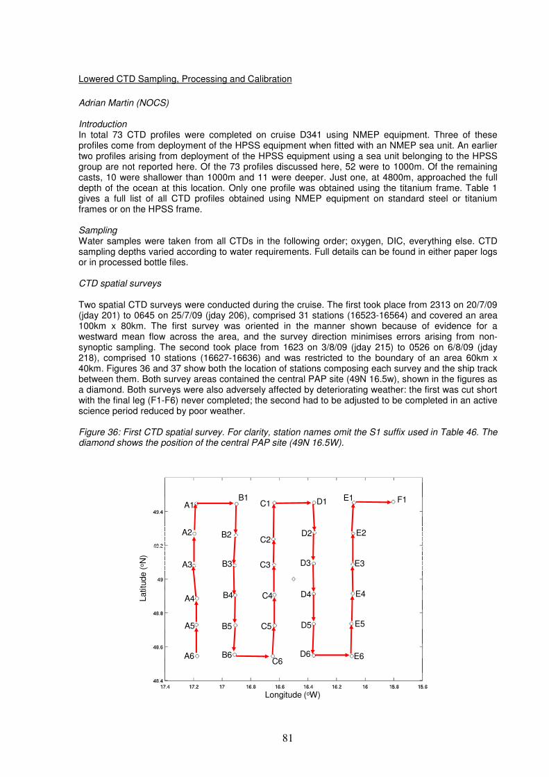
81
Lowered CTD Sampling, Processing and Calibration
Adrian Martin (NOCS) Introduction In total 73 CTD profiles were completed on cruise D341 using NMEP equipment. Three of these profiles come from deployment of the HPSS equipment when fitted with an NMEP sea unit. An earlier two profiles arising from deployment of the HPSS equipment using a sea unit belonging to the HPSS group are not reported here. Of the 73 profiles discussed here, 52 were to 1000m. Of the remaining casts, 10 were shallower than 1000m and 11 were deeper. Just one, at 4800m, approached the full depth of the ocean at this location. Only one profile was obtained using the titanium frame. Table 1 gives a full list of all CTD profiles obtained using NMEP equipment on standard steel or titanium frames or on the HPSS frame. Sampling Water samples were taken from all CTDs in the following order; oxygen, DIC, everything else. CTD sampling depths varied according to water requirements. Full details can be found in either paper logs or in processed bottle files. CTD spatial surveys Two spatial CTD surveys were conducted during the cruise. The first took place from 2313 on 20/7/09 (jday 201) to 0645 on 25/7/09 (jday 206), comprised 31 stations (16523-16564) and covered an area 100km x 80km. The first survey was oriented in the manner shown because of evidence for a westward mean flow across the area, and the survey direction minimises errors arising from non-synoptic sampling. The second took place from 1623 on 3/8/09 (jday 215) to 0526 on 6/8/09 (jday 218), comprised 10 stations (16627-16636) and was restricted to the boundary of an area 60km x 40km. Figures 36 and 37 show both the location of stations composing each survey and the ship track between them. Both survey areas contained the central PAP site (49N 16.5w), shown in the figures as a diamond. Both surveys were also adversely affected by deteriorating weather: the first was cut short with the final leg (F1-F6) never completed; the second had to be adjusted to be completed in an active science period reduced by poor weather. Figure 36: First CTD spatial survey. For clarity, station names omit the S1 suffix used in Table 46. The diamond shows the position of the central PAP site (49N 16.5W).
Latitu
de (
oN
)
Longitude (oW)
A1
A2
A3
A4
A5
A6
B1
B2
B3
B4
B5
B6
C1
C2
C3
C4
C5
C6
D1
D2
D3
D4
D5
D6
E1
E2
E3
E4
E5
E6
F1
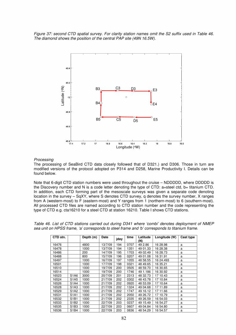
82
Figure 37: second CTD spatial survey. For clarity station names omit the S2 suffix used in Table 46. The diamond shows the position of the central PAP site (49N 16.5W).
Latitu
de (
oN
)
Longitude (oW)
E5
E4
E3
D5C5B5
B4
B3 C3 D3
Processing The processing of SeaBird CTD data closely followed that of D321.) and D306. Those in turn are modified versions of the protocol adopted on P314 and D258, Marine Productivity I. Details can be found below. Note that 6-digit CTD station numbers were used throughout the cruise – NDDDDD, where DDDDD is the Discovery number and N is a code letter denoting the type of CTD: a=steel ctd, b= titanium CTD. In addition, each CTD forming part of the mesoscale surveys was given a separate code denoting location in the survey – SqXY, where S denotes CTD survey, q denotes the survey number, X ranges from A (western-most) to F (eastern-most) and Y ranges from 1 (northern-most) to 6 (southern-most). All processed CTD files are named according to CTD station number and the code representing the type of CTD e.g. cta16210 for a steel CTD at station 16210. Table I shows CTD stations. Table 46. List of CTD stations carried out during D341 where ‘combi’ denotes deployment of NMEP sea unit on HPSS frame, ‘a’ corresponds to steel frame and ‘b’ corresponds to titanium frame.
CTD stn. Depth (m) Date jday
time Latitude (N)
Longitude (W) Cast type
16476 4800 13/7/09 194 0707 49 2.86 16 28.98 a 16478 1000 13/7/09 194 1351 49 01.33 16 28.38 a 16486 200 14/7/09 195 1703 49 02.49 16 28.73 a 16488 800 15/7/09 196 0207 49 01.08 16 31.91 a 16497 1000 16/7/09 197 1055 48 58.55 16 24.493 a 16501 1000 17/7/09 198 0321 48 49.65 16 35.21 a 16510 1000 19/7/09 200 0505 48 59.70 16 30.65 a 16514 1000 19/7/09 200 1746 49 1.186 16 30.92 a 16523 S1A6 3000 20/7/09 201 2313 48 32.73 17 10.43 a 16524 S1A5 1000 21/7/09 202 0302 48 43.78 17 10.84 a 16526 S1A4 1000 21/7/09 202 0920 48 53.09 17 10.64 a 16528 S1A3 1000 21/7/09 202 1324 49 04.68 17 11.89 a 16529 S1A2 1000 21/7/09 202 1747 49 16.12 17 11.66 a 16531 S1A1 1000 21/7/09 202 2050 49 26.72 17 10.79 a 16532 S1B1 1000 21/7/09 202 2335 49 26.59 16 54.03 a 16533 S1B2 1000 22/7/09 203 0237 49 15.49 16 54.27 a 16535 S1B3 1000 22/7/09 203 0607 49 04.84 16 54.80 a 16536 S1B4 1000 22/7/09 203 0836 48 54.29 16 54.57 a
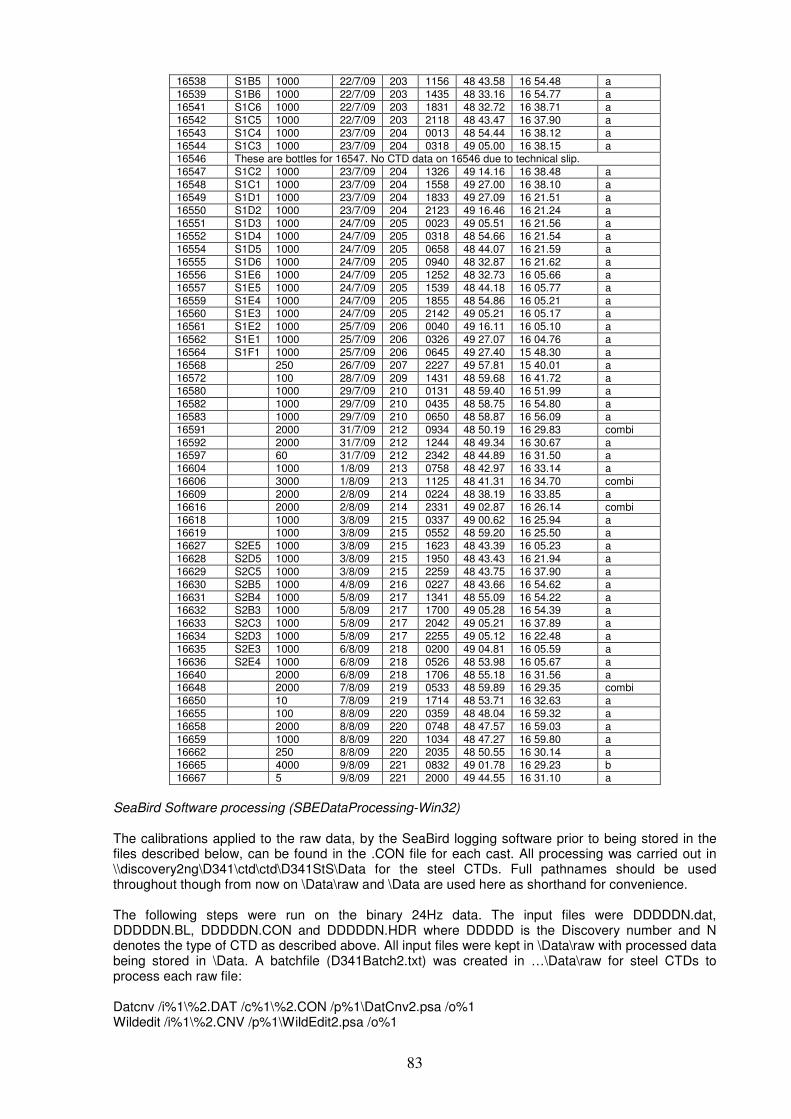
83
16538 S1B5 1000 22/7/09 203 1156 48 43.58 16 54.48 a 16539 S1B6 1000 22/7/09 203 1435 48 33.16 16 54.77 a 16541 S1C6 1000 22/7/09 203 1831 48 32.72 16 38.71 a 16542 S1C5 1000 22/7/09 203 2118 48 43.47 16 37.90 a 16543 S1C4 1000 23/7/09 204 0013 48 54.44 16 38.12 a 16544 S1C3 1000 23/7/09 204 0318 49 05.00 16 38.15 a 16546 These are bottles for 16547. No CTD data on 16546 due to technical slip. 16547 S1C2 1000 23/7/09 204 1326 49 14.16 16 38.48 a 16548 S1C1 1000 23/7/09 204 1558 49 27.00 16 38.10 a 16549 S1D1 1000 23/7/09 204 1833 49 27.09 16 21.51 a 16550 S1D2 1000 23/7/09 204 2123 49 16.46 16 21.24 a 16551 S1D3 1000 24/7/09 205 0023 49 05.51 16 21.56 a 16552 S1D4 1000 24/7/09 205 0318 48 54.66 16 21.54 a 16554 S1D5 1000 24/7/09 205 0658 48 44.07 16 21.59 a 16555 S1D6 1000 24/7/09 205 0940 48 32.87 16 21.62 a 16556 S1E6 1000 24/7/09 205 1252 48 32.73 16 05.66 a 16557 S1E5 1000 24/7/09 205 1539 48 44.18 16 05.77 a 16559 S1E4 1000 24/7/09 205 1855 48 54.86 16 05.21 a 16560 S1E3 1000 24/7/09 205 2142 49 05.21 16 05.17 a 16561 S1E2 1000 25/7/09 206 0040 49 16.11 16 05.10 a 16562 S1E1 1000 25/7/09 206 0326 49 27.07 16 04.76 a 16564 S1F1 1000 25/7/09 206 0645 49 27.40 15 48.30 a 16568 250 26/7/09 207 2227 49 57.81 15 40.01 a 16572 100 28/7/09 209 1431 48 59.68 16 41.72 a 16580 1000 29/7/09 210 0131 48 59.40 16 51.99 a 16582 1000 29/7/09 210 0435 48 58.75 16 54.80 a 16583 1000 29/7/09 210 0650 48 58.87 16 56.09 a 16591 2000 31/7/09 212 0934 48 50.19 16 29.83 combi 16592 2000 31/7/09 212 1244 48 49.34 16 30.67 a 16597 60 31/7/09 212 2342 48 44.89 16 31.50 a 16604 1000 1/8/09 213 0758 48 42.97 16 33.14 a 16606 3000 1/8/09 213 1125 48 41.31 16 34.70 combi 16609 2000 2/8/09 214 0224 48 38.19 16 33.85 a 16616 2000 2/8/09 214 2331 49 02.87 16 26.14 combi 16618 1000 3/8/09 215 0337 49 00.62 16 25.94 a 16619 1000 3/8/09 215 0552 48 59.20 16 25.50 a 16627 S2E5 1000 3/8/09 215 1623 48 43.39 16 05.23 a 16628 S2D5 1000 3/8/09 215 1950 48 43.43 16 21.94 a 16629 S2C5 1000 3/8/09 215 2259 48 43.75 16 37.90 a 16630 S2B5 1000 4/8/09 216 0227 48 43.66 16 54.62 a 16631 S2B4 1000 5/8/09 217 1341 48 55.09 16 54.22 a 16632 S2B3 1000 5/8/09 217 1700 49 05.28 16 54.39 a 16633 S2C3 1000 5/8/09 217 2042 49 05.21 16 37.89 a 16634 S2D3 1000 5/8/09 217 2255 49 05.12 16 22.48 a 16635 S2E3 1000 6/8/09 218 0200 49 04.81 16 05.59 a 16636 S2E4 1000 6/8/09 218 0526 48 53.98 16 05.67 a 16640 2000 6/8/09 218 1706 48 55.18 16 31.56 a 16648 2000 7/8/09 219 0533 48 59.89 16 29.35 combi 16650 10 7/8/09 219 1714 48 53.71 16 32.63 a 16655 100 8/8/09 220 0359 48 48.04 16 59.32 a 16658 2000 8/8/09 220 0748 48 47.57 16 59.03 a 16659 1000 8/8/09 220 1034 48 47.27 16 59.80 a 16662 250 8/8/09 220 2035 48 50.55 16 30.14 a 16665 4000 9/8/09 221 0832 49 01.78 16 29.23 b 16667 5 9/8/09 221 2000 49 44.55 16 31.10 a
SeaBird Software processing (SBEDataProcessing-Win32) The calibrations applied to the raw data, by the SeaBird logging software prior to being stored in the files described below, can be found in the .CON file for each cast. All processing was carried out in \\discovery2ng\D341\ctd\ctd\D341StS\Data for the steel CTDs. Full pathnames should be used throughout though from now on \Data\raw and \Data are used here as shorthand for convenience. The following steps were run on the binary 24Hz data. The input files were DDDDDN.dat, DDDDDN.BL, DDDDDN.CON and DDDDDN.HDR where DDDDD is the Discovery number and N denotes the type of CTD as described above. All input files were kept in \Data\raw with processed data being stored in \Data. A batchfile (D341Batch2.txt) was created in …\Data\raw for steel CTDs to process each raw file: Datcnv /i%1\%2.DAT /c%1\%2.CON /p%1\DatCnv2.psa /o%1 Wildedit /i%1\%2.CNV /p%1\WildEdit2.psa /o%1
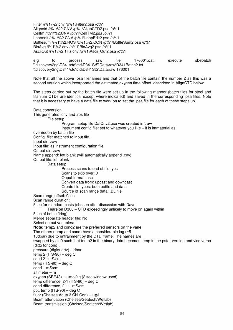
84
Filter /i%1\%2.cnv /p%1\Filter2.psa /o%1 Alignctd /i%1\%2.CNV /p%1\AlignCTD2.psa /o%1 Celltm /i%1\%2.CNV /p%1\CellTM2.psa /o%1 Loopedit /i%1\%2.CNV /p%1\LoopEdit2.psa /o%1 Bottlesum /i%1\%2.ROS /c%1\%2.CON /p%1\BottleSum2.psa /o%1 BinAvg /i%1\%2.cnv /p%1\BinAvg2.psa /o%1 AsciiOut /i%1\%2.1Hz.cnv /p%1\Ascii_Out2.psa /o%1 e.g to process raw file 176001.dat, execute sbebatch \\discovery2ng\D341\ctd\ctd\D341StS\Data\raw\D341Batch2.txt \\discovery2ng\D341\ctd\ctd\D341StS\Data\raw 176001 Note that all the above .psa filenames and that of the batch file contain the number 2 as this was a second version which incorporated the estimated oxygen time offset, described in AlignCTD below. The steps carried out by the batch file were set up in the following manner (batch files for steel and titanium CTDs are identical except where indicated) and saved in the corresponding .psa files. Note that it is necessary to have a data file to work on to set the .psa file for each of these steps up. Data conversion This generates .cnv and .ros file File setup Program setup file DatCnv2.psu was created in \raw Instrument config file: set to whatever you like – it is immaterial as overridden by batch file Config. file: matched to input file. Input dir: \raw Input file: as instrument configuration file Output dir: \raw Name append: left blank (will automatically append .cnv) Output file: left blank Data setup Process scans to end of file: yes Scans to skip over: 0 Ouput format: ascii Convert data from: upcast and downcast Create file types: both bottle and data Source of scan range data: .BL file Scan range offset: 0sec Scan range duration: 5sec for standard casts (chosen after discussion with Dave Teare on D306 – CTD exceedingly unlikely to move on again within 5sec of bottle firing) Merge separate header file: No Select output variables: Note: temp2 and cond2 are the preferred sensors on the vane. The others (temp and cond) have a considerable lag (~5- 10dbar) due to entrainment by the CTD frame. The names are swapped by ctd0 such that temp2 in the binary data becomes temp in the pstar version and vice versa (ditto for cond). pressure (digiquartz) – dbar temp 2 (ITS-90) – deg C cond 2– mS/cm temp (ITS-90) – deg C cond – mS/cm altimeter – m oxygen (SBE43) – mol/kg (2 sec window used) temp difference, 2-1 (ITS-90) – deg C cond difference, 2-1 – mS/cm pot. temp (ITS-90) – deg C fluor (Chelsea Aqua 3 Chl Con) – g/l Beam attenuation (Chelsea/Seatech/Wetlab) Beam transmission (Chelsea/Seatech/Wetlab)
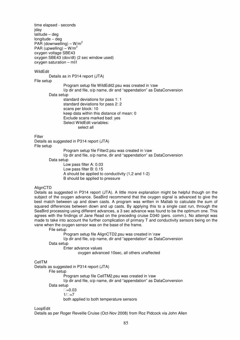
85
time elapsed - seconds jday latitude – deg longitude – deg PAR (downwelling) – W/m
2
PAR (upwelling) – W/m2
oxygen voltage SBE43 oxygen SBE43 (dov/dt) (2 sec window used) oxygen saturation – ml/l WildEdit Details as in P314 report (JTA) File setup Program setup file WildEdit2.psu was created in \raw I/p dir and file, o/p name, dir and “appendation” as DataConversion Data setup standard deviations for pass 1: 1 standard deviations for pass 2: 2 scans per block: 10 keep data within this distance of mean: 0 Exclude scans marked bad: yes Select WildEdit variables: select all Filter Details as suggested in P314 report (JTA) File setup Program setup file Filter2.psu was created in \raw I/p dir and file, o/p name, dir and “appendation” as DataConversion Data setup Low pass filter A: 0.03 Low pass filter B: 0.15 A should be applied to conductivity (1,2 and 1-2) B should be applied to pressure AlignCTD Details as suggested in P314 report (JTA). A little more explanation might be helpful though on the subject of the oxygen advance. SeaBird recommend that the oxygen signal is advanced to give the best match between up and down casts. A program was written in Matlab to calculate the sum of squared differences between down and up casts. By applying this to a single cast run, through the SeaBird processing using different advances, a 3 sec advance was found to be the optimum one. This agrees with the findings of Jane Read on the preceding cruise D340 (pers. comm.). No attempt was made to take into account the further complication of primary T and conductivity sensors being on the vane when the oxygen sensor was on the base of the frame. File setup Program setup file AlignCTD2.psu was created in \raw I/p dir and file, o/p name, dir and “appendation” as DataConversion Data setup Enter advance values oxygen advanced 10sec, all others unaffected CellTM Details as suggested in P314 report (JTA) File setup Program setup file CellTM2.psu was created in \raw I/p dir and file, o/p name, dir and “appendation” as DataConversion Data setup =0.03 1/=7 both applied to both temperature sensors LoopEdit Details as per Roger Reveille Cruise (Oct-Nov 2008) from Roz Pidcock via John Allen
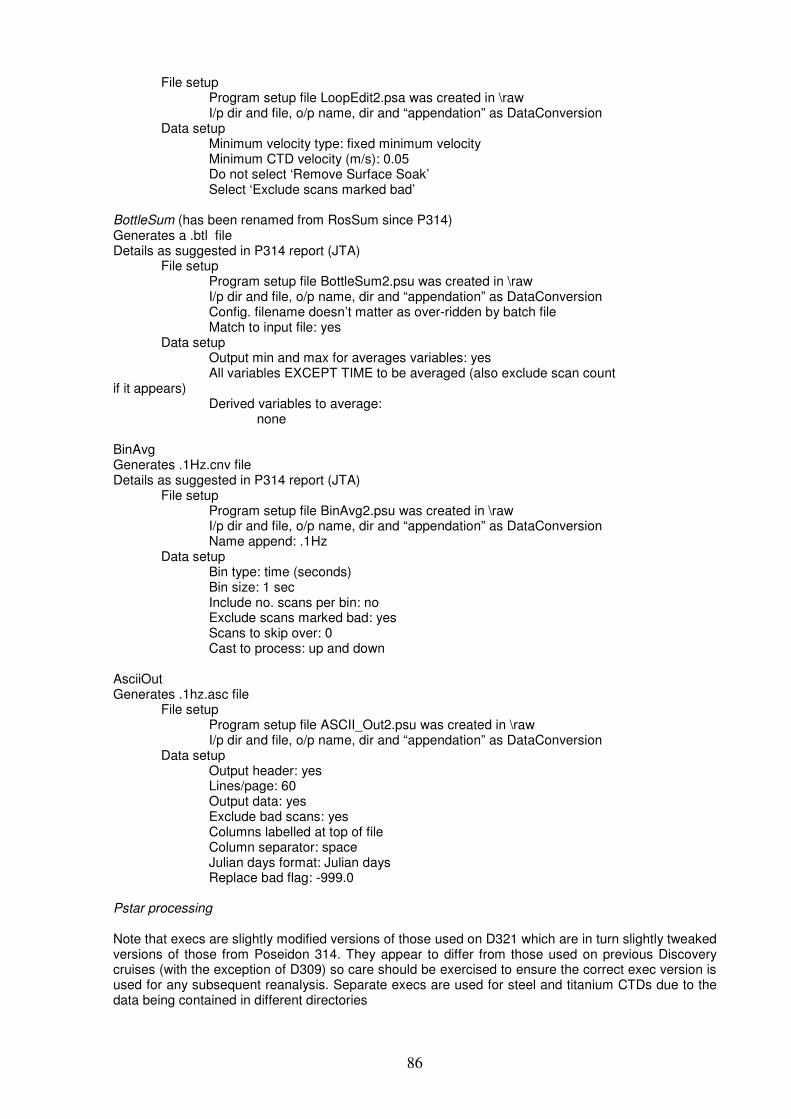
86
File setup Program setup file LoopEdit2.psa was created in \raw I/p dir and file, o/p name, dir and “appendation” as DataConversion Data setup Minimum velocity type: fixed minimum velocity Minimum CTD velocity (m/s): 0.05 Do not select ‘Remove Surface Soak’ Select ‘Exclude scans marked bad’ BottleSum (has been renamed from RosSum since P314) Generates a .btl file Details as suggested in P314 report (JTA) File setup Program setup file BottleSum2.psu was created in \raw I/p dir and file, o/p name, dir and “appendation” as DataConversion Config. filename doesn’t matter as over-ridden by batch file Match to input file: yes Data setup Output min and max for averages variables: yes All variables EXCEPT TIME to be averaged (also exclude scan count if it appears) Derived variables to average: none BinAvg Generates .1Hz.cnv file Details as suggested in P314 report (JTA) File setup Program setup file BinAvg2.psu was created in \raw I/p dir and file, o/p name, dir and “appendation” as DataConversion Name append: .1Hz Data setup Bin type: time (seconds) Bin size: 1 sec Include no. scans per bin: no Exclude scans marked bad: yes Scans to skip over: 0 Cast to process: up and down AsciiOut Generates .1hz.asc file File setup Program setup file ASCII_Out2.psu was created in \raw I/p dir and file, o/p name, dir and “appendation” as DataConversion Data setup Output header: yes Lines/page: 60 Output data: yes Exclude bad scans: yes Columns labelled at top of file Column separator: space Julian days format: Julian days Replace bad flag: -999.0 Pstar processing Note that execs are slightly modified versions of those used on D321 which are in turn slightly tweaked versions of those from Poseidon 314. They appear to differ from those used on previous Discovery cruises (with the exception of D309) so care should be exercised to ensure the correct exec version is used for any subsequent reanalysis. Separate execs are used for steel and titanium CTDs due to the data being contained in different directories
87
ctd0S and ctd0T – translate the 24Hz SeaBird DDDDDN.cnv file into pstar format. Require the latitude and longitude of the bottom of the cast. These are entered manually from details on the CTD log-sheet but can be automatically checked and corrected later on. Output ctNDDDDD.24hz ctd1S and ctd1T – after checking output of ctd0 with plxyed for spikes that may need to be removed before proceeding, ctd1S/T averages 24Hz data into 1Hz and derives salinity, potential temperature and density. It was noted that many of the casts had small spikes in both primary and secondary T and C sensors on the down cast, probably as a result of entrained water from slightly higher in the water column as this only was noticeable in the sharp gradient region of the seasonal thermocline. Output ctNDDDDD.1hz (and ctNDDDDD.10s) ctd2S and ctd2T – require the user to first find the first in-water, deepest and last in-water datacycle using plxyed (with ctd1Hz.pdf) prior to use. These execs then extract data corresponding to full up and down casts (ctNDDDDD.ctu) and purely the downcast (ctNDDDDD.2db) averaged into 2db bins. sam0S and sam0T – create a file, fir/fiNDDDDD, containing CTD data corresponding to the firing times of the bottles. It does so using the relevant .btl file in raw/. The resulting pstar file has both mean and standard deviation for all variables. sam1S and sam1T – create a sample file, saNDDDDD, containing both CTD data at bottle firing depths but also with space for variables for which samples were taken e.g. oxygen, nutrients, chlorophyll. The list of sampled variables is contained in sam.names. Note is also made at this stage of the number of bottles fired on each cast to ensure the ascii sample file (see Salinometry section of report) has only this number of rows. Asciiexec/frasciiexec – created ascii versions of ctNDDDDD.2db (as fulascNDDDDD.txt) and saNDDDDD (as botascNDDDDD.txt) for use buy ther scientists on cruise. The two versions of this program are for standard CTD (asciiexec) and for the French CTD when using NERC Sea Unit (frasciiexec). Salinity calibration and sensor issues Salinity samples were taken on 56 of the 70 CTD profiles conducted using an NMEP frame and rosette. Figs 38 and 39 show differences between salinometer derived bottle sampled salinities and those derived from continuous CTD data. To remove outliers the differences between bottle and CTD estimated salinity were twice screened to exclude data-points outside 2 standard deviations of the mean. It is apparent that even this was not fully successful. For the primary sensor the mean offset is less than 0.001 psu. There is no trend with time but there is much variability throughout the cruise. In particular the periods of the two mesoscale surveys show the most scatter. There are two potential causes: first, the intensive nature of the survey required sampling by people both inexperienced in salinity sampling and also coming from different institutes which may have different protocols; second, the weather deteriorated during each survey so there is a potential rainwater signal for samples taken by less experienced samplers.

88
Figure 38: Differences (psu) between bottle and primary CTD salinity sensor
The same pattern is seen in residuals for the secondary salinity sensor. The mean residual is a ittle higher though at 0.0022 psu. Generally the residuals for both sensors are acceptable for a multidisciplinary exercise of this nature where there is not intent to infer subtle shifts in water mass characteristics. Further attention to specific remaining outliers and trends among samplers will hopefully reduce the standard deviation. This currently exaggerates the variability by virtue of the strong non-Gaussianity of residuals seen in the figures. Figure 39. Differences (psu) between bottle and secondary CTD salinity sensor
89
Vessell Mounted ADCP (VM-ADCP) and navigation data John Allen, NOCS
1. Introduction During the refit for RRS Discovery in March 2008, the original narrow band RDI 150 kHz Vessel-Mounted Acoustic Doppler Current Profiler (VM-ADCP) was replaced with an RDI broad band 150 kHz (Ocean Surveyor) phased array style VM-ADCP. This was in addition to the similar 75 kHz Ocean Surveyor instrument that had been in use in the forward ADCP housing since 2001. The 150 kHz ADCP is mounted in the hull 1.75 m to port of the keel, 33 m aft of the bow at the waterline and at an approximate depth of 5 m. The 75 kHz ADCP is also mounted in the hull, but in a second water chest 4.15 m forward and 2.5 m to starboard of the 150 kHz well. This section describes the operation and data processing paths for both ADCPs. The navigation data processing is described first since it is key to the accuracy of the ADCP current data. All integrated underway data were logged using the Ifremer TechSAS data logging system that has been gradually implemented on RRS Discovery for approximately 3 years. The extensive NMFSS scripts to read the netcdf format TechSAS file streams and create RVS data streams have been developed alongside the implementation of the system and most errors and wrinkles have been worked out. The ‘live’ RVS data format streams have overcome the problem discussed in some recent reports of insufficient significant figure resolution in position data using nclistit. Apparently these do not convert the netcdf format to RVS data format, instead, they log TechSAS broadcast messages independently.
2. Navigation The ship’s primary position instrument was the GPS Trimble 4000 system. The positional accuracy for the GPS 4000 system was determined from the data recovered whilst tied up alongside in KGV docks, Govan. Standard deviation for positional accuracy was an incredible 1.045 m in latitude and 0.612 m in longitude, and some of this maybe due to heave in the mooring lines. In comparison, the Ashtech G12 navigation system was a little less accurate with standard deviation for positional accuracy of 2.000 m in latitude and 1.198 m in longitude. Both navigations systems therefore had sufficient precision to enable the calculation of ship's velocities to better than 1 cms
-1, and therefore below the instrumental limits (~ 1 cms
-1) of the RDI
ADCP systems. Using the GPS 4000 system as its primary navigation source, the NMFSS Bestnav combined (10 second) clean navigation process was operational on D341, however it returned a believable but spurious ship’s track for approximately 10 hours whilst rounding the south-east corner of Eire on passage out to the PAP site. The cause of this problem with Bestnav was never identified and therefore the raw Trimble GPS 4000 data were taken as the master navigation source all cruise. In point of fact, the Trimble, Ashtech and Bestnav files streams matched perfectly for the rest of the cruise, and the largest gap in the Trimble GPS 4000 data stream was 91 seconds. Navigation and gyro data were transferred daily from the RVS format file streams to pstar navigation files, e.g. abnv3401, gp434001 and gyr34001. Scripts: navexec0: transferred data from the RVS bestnav file to PSTAR, calculated the ships velocity, appended onto a cruise navigation file and calculated the distance run from the start of the file. Output: abnv3411 gyroexec0: transferred data from the RVS gyrol file stream to Pstar, a nominal edit was made for directions between 0-360° before the file was appended to a master file. Output: gyr34101 gps4exec0: transferred data from the RVS gps_4kl file stream to Pstar, edited out pdop (position dilution of precision) greater than 7 and appended the new 24 hour file to a master file. The master file was averaged to create an additional 30 second file and distance run was calculated and added to both. Output: gp434101 and gp434101.30sec gpsg12exec0: transferred data from the RVS gps_g12l file stream to Pstar, edited out pdop (position dilution of precision) greater than 7, appended the new 24 hour file to a master file and distance run was calculated. Output: gpsg1234101
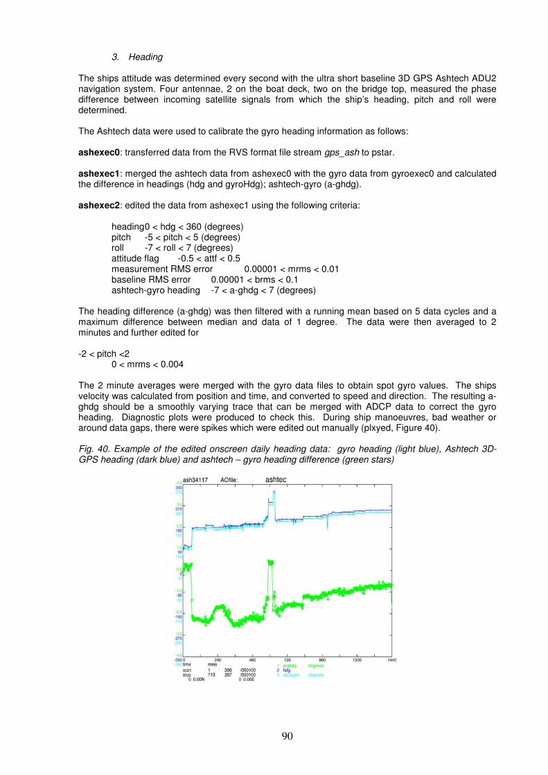
90
3. Heading
The ships attitude was determined every second with the ultra short baseline 3D GPS Ashtech ADU2 navigation system. Four antennae, 2 on the boat deck, two on the bridge top, measured the phase difference between incoming satellite signals from which the ship’s heading, pitch and roll were determined. The Ashtech data were used to calibrate the gyro heading information as follows: ashexec0: transferred data from the RVS format file stream gps_ash to pstar. ashexec1: merged the ashtech data from ashexec0 with the gyro data from gyroexec0 and calculated the difference in headings (hdg and gyroHdg); ashtech-gyro (a-ghdg). ashexec2: edited the data from ashexec1 using the following criteria: heading 0 < hdg < 360 (degrees) pitch -5 < pitch < 5 (degrees) roll -7 < roll < 7 (degrees) attitude flag -0.5 < attf < 0.5 measurement RMS error 0.00001 < mrms < 0.01 baseline RMS error 0.00001 < brms < 0.1 ashtech-gyro heading -7 < a-ghdg < 7 (degrees) The heading difference (a-ghdg) was then filtered with a running mean based on 5 data cycles and a maximum difference between median and data of 1 degree. The data were then averaged to 2 minutes and further edited for -2 < pitch <2 0 < mrms < 0.004 The 2 minute averages were merged with the gyro data files to obtain spot gyro values. The ships velocity was calculated from position and time, and converted to speed and direction. The resulting a-ghdg should be a smoothly varying trace that can be merged with ADCP data to correct the gyro heading. Diagnostic plots were produced to check this. During ship manoeuvres, bad weather or around data gaps, there were spikes which were edited out manually (plxyed, Figure 40). Fig. 40. Example of the edited onscreen daily heading data: gyro heading (light blue), Ashtech 3D-GPS heading (dark blue) and ashtech – gyro heading difference (green stars)
91
Ashtech 3D GPS coverage was generally good. Gaps over 1 minute in the data stream are listed below. (Table 47) Table 47. Gaps in Ashtech data
4. VM-ADCP data This section would normally describe the operation and data processing paths for both ADCPs fitted to RRS Discovery. However, before reaching the PAP study site, it was clear that the 75 kHz ADCP had ceased to provide any current data and very little return signal strength was being detected by either the transducers or the deck unit. Thorough diagnostic checks indicated potential problems with ADCP instrument itself, but email communication of the diagnostic results to RDI led the manufacturers to suggest that the deck unit would need to be repaired. Thus only the 150 kHz VM-ADCP was operable during this cruise. Interestingly, our initial thoughts were that there might be air in the 75 kHz VM-ADCP housing. This is normally continuously bled through a small bleed valve to a stanchion pipe at deck level. Investigations showed that the bleed channel had indeed blocked up below the bleed valve. This blockage was cleared with high pressure air by the engineering staff, until water began to flow. Sadly, on this occasion, this did not solve the VM-ADCP problem and hence we began the diagnostic checks. 150 kHz VM-ADCP data processing The RDI Ocean Surveyor 150 kHz Phased Array VM-ADCP was configured to sample over 120 second intervals with 100 bins of 4m depth and a blank beyond transmit of distance of 4m. The instrument is a broad-band phased array ADCP with 153.6 kHz frequency and a 30° beam angle. Both deck units had firmware upgrades to VMDAS 23.17 after the March 2008 refit. Both control PCs ran RDI software VmDAS v1.46. Gyro heading, and GPS Ashtech heading, location and time were fed as NMEA messages into the serial ports of the both PCs and VmDAS was configured to use the Gyro heading for co-ordinate transformation. VmDAS logs the PC clock time, stamps the data (start of each ensemble) with that time, and records the offset of the PC clock from GPS time. This offset was applied to the data in the processing path before merging with navigation. The 2 minute averaged data were written to the PC hard disk in files with a .STA extension, eg D341os150001_000000.STA, D341os150002_000000.STA etc. Sequentially numbered files were created whenever data logging was stopped and re-started. The software was set to close the file once it reached 100MB in size, though on D341 files were closed and data collection restarted daily such that the files never became that large. All files were transferred to the unix directories /data32/d341/os150/raw. This transfer included the plethora of much larger ping by ping data files, these can be useful in the event of major failure of the ship’s data handling systems as they record all the basic navigation and ships heading/attitude data supplied by NMEA message. The VM-ADCP instrument was configured to run in ‘Narrowband’ range over resolution mode. Bottom tracking was used until we left the continental shelf at the Porcupine sea bight. Bottom tracking was also used as we returned across the continental shelf south of Eire. The VM-ADCP processing path followed an identical route to that developed in 2001 for the 75 kHz ADCP (RRS Discovery cruise 253). In the following script descriptions, “##” indicates the daily file number. s150exec0: data read into Pstar format from RDI binary file (psurvey2). Water track velocities written into “adp” files, bottom track into “bot” files if in bottom track mode. Velocities were scaled to cm/s and amplitude by 0.45 to db. The time variable was corrected to GPS time by combining the PC clock time
time gap : 09 186 15:52:18 to 09 186 15:53:30 (72 s) time gap : 09 188 08:25:28 to 09 188 08:26:29 (61 s) time gap : 09 192 13:03:56 to 09 192 13:04:57 (61 s) time gap : 09 192 13:10:42 to 09 192 13:11:47 (65 s) time gap : 09 203 21:06:41 to 09 203 21:08:16 (95 s) time gap : 09 206 11:07:43 to 09 206 11:08:50 (67 s) time gap : 09 217 01:50:40 to 09 217 01:51:42 (62 s) time gap : 09 220 23:07:14 to 09 220 23:08:18 (64 s) time gap : 09 223 20:48:59 to 09 223 20:50:14 (75 s)
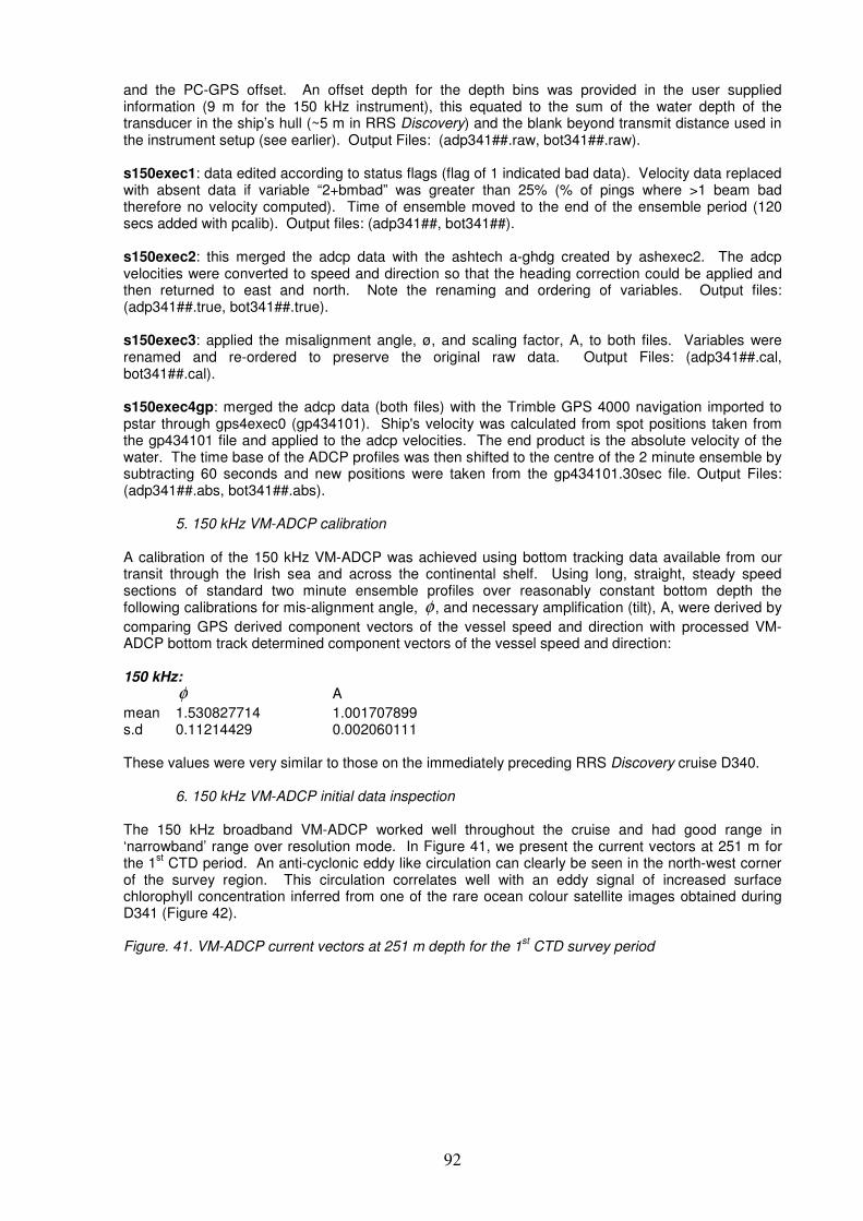
92
and the PC-GPS offset. An offset depth for the depth bins was provided in the user supplied information (9 m for the 150 kHz instrument), this equated to the sum of the water depth of the transducer in the ship’s hull (~5 m in RRS Discovery) and the blank beyond transmit distance used in the instrument setup (see earlier). Output Files: (adp341##.raw, bot341##.raw). s150exec1: data edited according to status flags (flag of 1 indicated bad data). Velocity data replaced with absent data if variable “2+bmbad” was greater than 25% (% of pings where >1 beam bad therefore no velocity computed). Time of ensemble moved to the end of the ensemble period (120 secs added with pcalib). Output files: (adp341##, bot341##). s150exec2: this merged the adcp data with the ashtech a-ghdg created by ashexec2. The adcp velocities were converted to speed and direction so that the heading correction could be applied and then returned to east and north. Note the renaming and ordering of variables. Output files: (adp341##.true, bot341##.true). s150exec3: applied the misalignment angle, ø, and scaling factor, A, to both files. Variables were renamed and re-ordered to preserve the original raw data. Output Files: (adp341##.cal, bot341##.cal). s150exec4gp: merged the adcp data (both files) with the Trimble GPS 4000 navigation imported to pstar through gps4exec0 (gp434101). Ship's velocity was calculated from spot positions taken from the gp434101 file and applied to the adcp velocities. The end product is the absolute velocity of the water. The time base of the ADCP profiles was then shifted to the centre of the 2 minute ensemble by subtracting 60 seconds and new positions were taken from the gp434101.30sec file. Output Files: (adp341##.abs, bot341##.abs).
5. 150 kHz VM-ADCP calibration A calibration of the 150 kHz VM-ADCP was achieved using bottom tracking data available from our transit through the Irish sea and across the continental shelf. Using long, straight, steady speed sections of standard two minute ensemble profiles over reasonably constant bottom depth the following calibrations for mis-alignment angle, φ , and necessary amplification (tilt), A, were derived by
comparing GPS derived component vectors of the vessel speed and direction with processed VM-ADCP bottom track determined component vectors of the vessel speed and direction: 150 kHz:
φ A
mean 1.530827714 1.001707899 s.d 0.11214429 0.002060111 These values were very similar to those on the immediately preceding RRS Discovery cruise D340.
6. 150 kHz VM-ADCP initial data inspection
The 150 kHz broadband VM-ADCP worked well throughout the cruise and had good range in ‘narrowband’ range over resolution mode. In Figure 41, we present the current vectors at 251 m for the 1
st CTD period. An anti-cyclonic eddy like circulation can clearly be seen in the north-west corner
of the survey region. This circulation correlates well with an eddy signal of increased surface chlorophyll concentration inferred from one of the rare ocean colour satellite images obtained during D341 (Figure 42). Figure. 41. VM-ADCP current vectors at 251 m depth for the 1
st CTD survey period
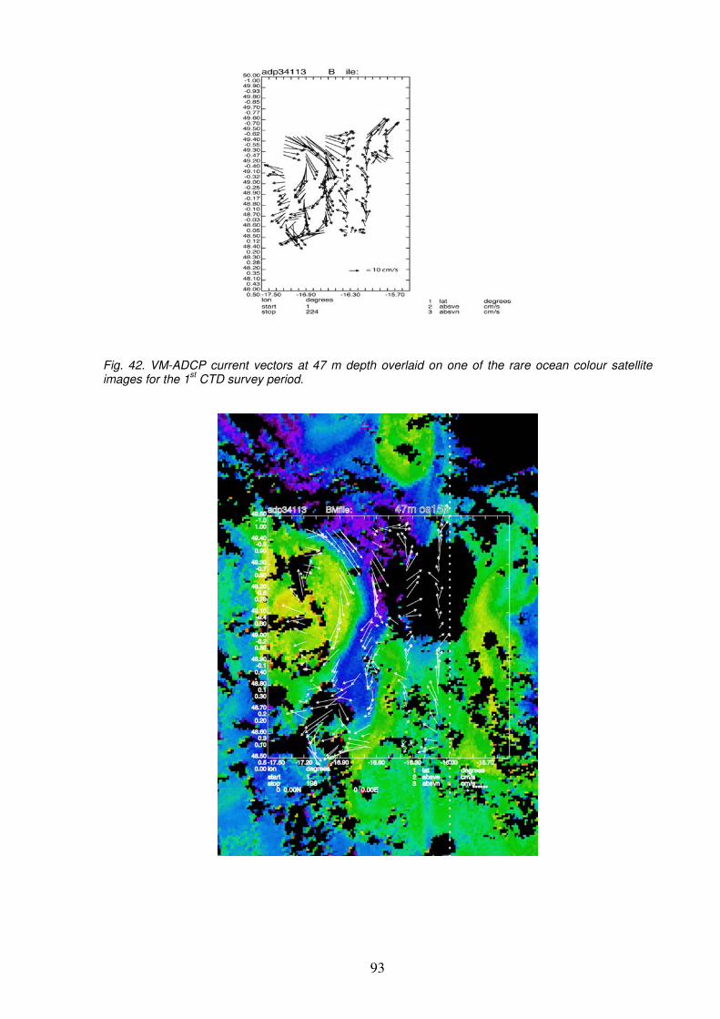
93
Fig. 42. VM-ADCP current vectors at 47 m depth overlaid on one of the rare ocean colour satellite images for the 1
st CTD survey period.
94
Giering net and ARIES samples Sari Giering, (Then Aberdeen, now NOCS)
1. Background
Zooplankton plays a major role in the biological carbon pump. They feed on phytoplankton and smaller organisms in the surface waters during night time and migrate downwards during day time. This daily vertical migration results in an active transport of carbon into depths through both respiration and excretion. The accurate quantification of mesozooplanktonic carbon consumption is essential for the understanding of the role of mesozooplankton in the pelagic biogeochemistry and the process of the biological carbon pump. The quantity of zooplanktonic carbon transport is estimated using zooplankton metabolic rates such as respiration rates and carbon demand. Conventionally, zooplanktonic carbon demand (ZCD) is calculated on the base of size fractured biomass and water temperature (Ikeda, 1987). The animals are sampled from several discrete depth intervals and converted into zooplankton respiration (ZR) and ZCD using two equations:
TaBMaaZR 210 lnln ++= , (1)
where ln is the natural logarithm, ZR is the respiration rate (µL O2 individual
-1 h
-1), BM is the body
mass (mg dry weight, C, N, or P wt individual-1
), T is the habitat temperature (°C) and a0, a1 and a2 are constants.
AER
ZRZCD
⋅= , (2)
where ZCD is measured in mg C m
-2 d
-1, ZR is the respiration rate converted into carbon equivalents
(mg C m-2
d-1
) after Al-Mutairi and Landry (2001), R is the fraction of assimilated carbon that is respired
(~50%; Ikeda 1987), and AE is the fraction of carbon consumed that was assimilated (50-70%; Steinberg et al. 1997). The zooplankton respiration model accounts for 84-96% of the variation in respiration rates. Therefore, additional feeding experiments are required to confirm the model output. 2. Aries
To estimate the carbon demand of the zooplankton between 0 – 1000 m depth, the mesozooplankton at the PAP zone was sampled using an Autosampling and Recording Instrumented Environmental Sampling System (ARIES). ARIES can take 110 samples from discrete depth intervals with a 200 µm net. Due to sample size the downcast samples are less useful for quantitative analysis; however they can be used for biogeochemical analysis. The upcast samples are quantitative and give a good representation of the zooplankton community at the sampled depth range. Using the equations described above, the samples will be converted into zooplankton carbon demand. ARIES was deployed at different daytimes to give a full cover of the daily vertical migration and a better understanding of the species involved in active vertical carbon transport. 2.1 Aries Samples Eight ARIES deployments were conducted from 0 – 1000 m depth (Table 48). Individual ARIES cod-ends were carefully rinsed onto 200 µm mesh squares, which were folded and processed according to the cast. Downcast samples were wrapped in tin foil, labelled, put in polybags and stored at -70°C. Upcast samples were put into 30 mL glass vials containing 4% formaldehyde solution, labelled and stored. A total of 858 samples were taken: 443 downcast samples and 415 upcast samples. Furthermore, two 200 µm pop nets were placed on the ARIES main frame to collect an integrated sample over the entire depth range. One integrated sample was frozen, the other one preserved in 4% formaldehyde solution.
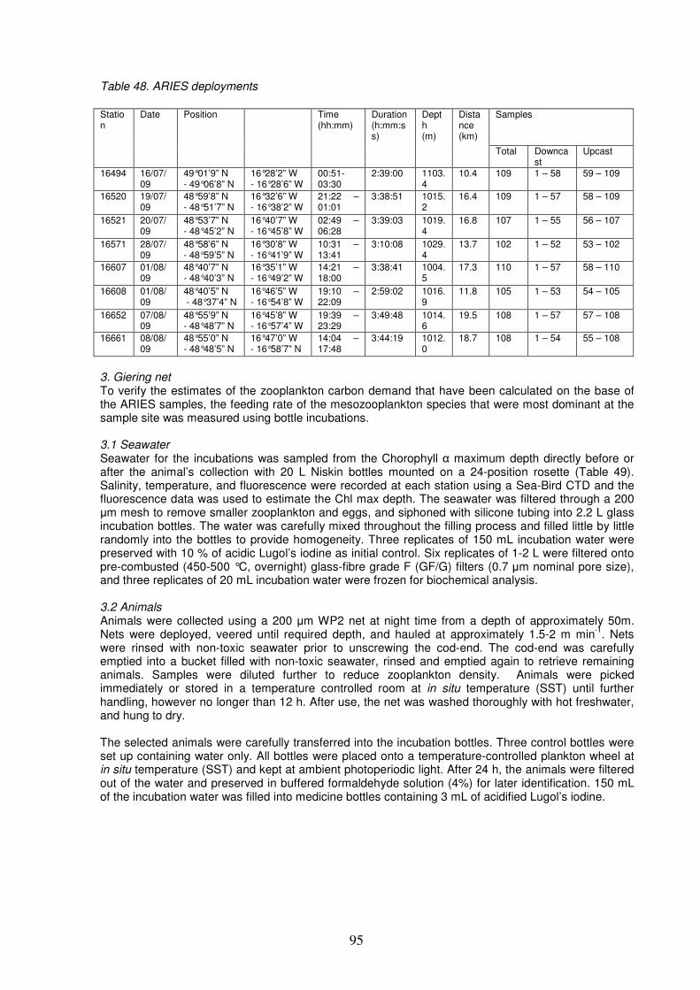
95
Table 48. ARIES deployments
3. Giering net To verify the estimates of the zooplankton carbon demand that have been calculated on the base of the ARIES samples, the feeding rate of the mesozooplankton species that were most dominant at the sample site was measured using bottle incubations. 3.1 Seawater Seawater for the incubations was sampled from the Chorophyll α maximum depth directly before or after the animal’s collection with 20 L Niskin bottles mounted on a 24-position rosette (Table 49). Salinity, temperature, and fluorescence were recorded at each station using a Sea-Bird CTD and the fluorescence data was used to estimate the Chl max depth. The seawater was filtered through a 200 µm mesh to remove smaller zooplankton and eggs, and siphoned with silicone tubing into 2.2 L glass incubation bottles. The water was carefully mixed throughout the filling process and filled little by little randomly into the bottles to provide homogeneity. Three replicates of 150 mL incubation water were preserved with 10 % of acidic Lugol’s iodine as initial control. Six replicates of 1-2 L were filtered onto pre-combusted (450-500 °C, overnight) glass-fibre grade F (GF/G) filters (0.7 µm nominal pore size), and three replicates of 20 mL incubation water were frozen for biochemical analysis. 3.2 Animals Animals were collected using a 200 µm WP2 net at night time from a depth of approximately 50m. Nets were deployed, veered until required depth, and hauled at approximately 1.5-2 m min
-1. Nets
were rinsed with non-toxic seawater prior to unscrewing the cod-end. The cod-end was carefully emptied into a bucket filled with non-toxic seawater, rinsed and emptied again to retrieve remaining animals. Samples were diluted further to reduce zooplankton density. Animals were picked immediately or stored in a temperature controlled room at in situ temperature (SST) until further handling, however no longer than 12 h. After use, the net was washed thoroughly with hot freshwater, and hung to dry. The selected animals were carefully transferred into the incubation bottles. Three control bottles were set up containing water only. All bottles were placed onto a temperature-controlled plankton wheel at in situ temperature (SST) and kept at ambient photoperiodic light. After 24 h, the animals were filtered out of the water and preserved in buffered formaldehyde solution (4%) for later identification. 150 mL of the incubation water was filled into medicine bottles containing 3 mL of acidified Lugol’s iodine.
Samples Station
Date Position Time (hh:mm)
Duration (h:mm:ss)
Depth (m)
Distance (km)
Total Downcast
Upcast
16494 16/07/09
49°01’9” N - 49°06’8” N
16°28’2” W - 16°28’6” W
00:51- 03:30
2:39:00 1103.4
10.4 109 1 – 58 59 – 109
16520 19/07/09
48°59’8” N - 48°51’7” N
16°32’6” W - 16°38’2” W
21:22 – 01:01
3:38:51 1015.2
16.4 109 1 – 57 58 – 109
16521 20/07/09
48°53’7” N - 48°45’2” N
16°40’7” W - 16°45’8” W
02:49 – 06:28
3:39:03 1019.4
16.8 107 1 – 55 56 – 107
16571 28/07/09
48°58’6” N - 48°59’5” N
16°30’8” W - 16°41’9” W
10:31 – 13:41
3:10:08 1029.4
13.7 102 1 – 52 53 – 102
16607 01/08/09
48°40’7” N - 48°40’3” N
16°35’1” W - 16°49’2” W
14:21 – 18:00
3:38:41 1004.5
17.3 110 1 – 57 58 – 110
16608 01/08/09
48°40’5” N - 48°37’4” N
16°46’5” W - 16°54’8” W
19:10 – 22:09
2:59:02 1016.9
11.8 105 1 – 53 54 – 105
16652 07/08/09
48°55’9” N - 48°48’7” N
16°45’8” W - 16°57’4” W
19:39 – 23:29
3:49:48 1014.6
19.5 108 1 – 57 57 – 108
16661 08/08/09
48°55’0” N - 48°48’5” N
16°47’0” W - 16°58’7” N
14:04 – 17:48
3:44:19 1012.0
18.7 108 1 – 54 55 – 108
96
3.3 Estimation of feeding rates The microplankton in the preserved incubation water samples will be analysed. Cells are identified and enumerated. The cell volume is determined, corrected for shrinkage induced by the preservation with Lugol’s iodine, and converted to carbon (Strathmann 1967, Ohman & Runge 1994). Clearance and ingestion rates are determined, and feeding preferences are examined. 3.4 Samples Nets were deployed at twelve stations and eight feeding experiments were carried out (Table 50). A total of 113 water samples were taken, five sets of pre-experimental animals were picked, 56 L water have been filtered onto 48 GF/G filter and frozen at -70°C, and eight sets of water samples (3 x 20 mL) were stored at -70°C. Additional four stations were sampled for zooplankton community analysis (Table 4). Samples were taken from 45 m, 85 m and 135 m depth and split. One sub-sample was frozen for fatty acid analysis and one preserved in formaldehyde solution (4%) for identification and quantification purposes. Furthermore, four samples of the most abundant species at station 16617 were picked and frozen for fatty acid analysis. Table 49. CTD casts collecting water for feeding experiments Table 50. WP2 net deployments for life samples
Station Date Position Cast On deck (hh:mm)
Depth (m)
16501 17/07/09 48°49’6” N 16°35’2” W 006 04:04 25 16510 19/07/09 48°59’9” N 16°30’6” W 007 05:59 25 16524 21/07/09 48°43’6” N 17°10’9” W 010 03:55 25 16535 22/07/09 49°04’3” N 16°55’0” W 017 06:44 25 16554 24/07/09 48°44’2” N 16°21’3” W 032 07:36 25 16564 25/07/09 49°27’8” N 15°47’8” W 040 07:23 25 16580 29/07/09 48°59’0” N 16°52’6” W 043 02:15 22 16597 31/07/09 48°44’7” N 16°31’7” W 048 23:51 29 16618 03/08/09 49°00’2” N 16°25’6” W 053 04:10 25 16659 08/08/09 48°47’4” N 16°59’8” W 068 10:08 25
Station
Date Position Time (hh:mm)
Depth (m)
Exp.
Date Spp. (replicates)
16480/1
14/07/09
49°01’8” N
16°29’3” W
09:30 – 10:04
100 * * *
16492 15/07/09
49°03’8” N
16°33’2” W
08:42 – 09:31
100 * * *
16500 17/07/09
48°49’6” N
16°31’7” W
23:53 – 00:26
50 1 17-18/07/09 Parapseudocalanus (3), Arcatia (3), Metridia (3)
16511 19/07/09
48°59’1” N
16°30’6” W
06:45 – 07:38
80 2 19-20/07/09 Parapseudocalanus (3), Arcatia (3), Metridia (?) (3)
16525 21/07/09
48°43’5” N
17°11’0” W
05:25 – 05:55
75 3 21-22/07/09 Mixed spp., ≥500 µm (3)
16534 22/07/09
49°14’0” N
16°53’8” W
04:10 – 04:25
75 4 22-23/07/09 Mixed spp. (3,3) Influence of incubation water filter mesh size.
16553 24/07/09
48°54’8” N
16°21’5” W
04:33 – 04:50
50 5 24-25/07/09 Diff zooplankton spp. (1,1,4,2)
16563 25/07/09
49°27’6” N
16°03’9” W
04:30 – 04:50
40 * * *
16581 29/07/09
48°58’9” N
16°53’2” W
03:06 – 03:29
40 6 29-30/07/09 Calanus (1), Arcatia (5), Metridia (3)
16596 31/07/09
48°45’9” N
16°30’9” W
21:58 – 22:12
60 * * *
16617 03/08/09
49°01’8” N
16°25’8” W
02:10 – 02:38
50 7 03-04/08/09 Parapseudocalanus (3), Arcatia (5), Calanus (1)
16656 08/08/09
48°47’9” N
16°59’4” W
04:37 – 05:03
50 8 08-09/08/09

97
Table 51. WP2 net deployments for community analysis
Station Date Position Time (hh:mm)
Depths (m)
16596 31/07/09 48°45’9” N 16°30’9” W
22:05 – 22:25 45 85 135
16600-2 01/08/09 48°44’0” N 16°32’4” W
05:25 – 05:42 45 85 135
16617 03/08/09 49°01’8” N 16°25’8” W
01:32 – 02:10 45 85 135
16647 07/08/09 49°02’0” N 16°29’8” W
03:09 – 03:51 45 85 135
4. References Al-Mutairi H, Landry MR (2001) Active export of carbon and nitrogen at Station ALOHA by diel migrant zooplankton. Deep Sea Res II 48:2083-2103 Ikeda T (1987) Metabolic rates of epipelagic marine zooplankton as a function of body mass and temperature. Mar Biol 85:1-11 Ohman MD, Runge JA (1994) Sustained fecundity when phytoplankton resources are in short supply: omnivory by Calanus fonmarchicus in the Gulf of St. Lawrence. Limnol Oceanogr 23:21-36 Steinberg M, Silver W, Pilskaln CH (1997) Role of mesopelagic zooplankton in the community metabolism of giant larvacean house detritus in Monterey Bay, California, USA. Mar Ecol Prog Ser 147:167-179 Strathmann RR (1967) Estimating the organic carbon content of phytoplankton from cell volume or plasma volume. Limnol Oceanogr 12:411-418
98
PELAGRA – neutrally buoyant sediment traps (scientific) Chris Marsay (NOCS) One of the main aims of cruise D341 was to measure the downward flux of carbon and other elements, with PELAGRA providing one of the tools for achieving this aim. It was hoped that from each deployment, measurements could be made of particulate organic and inorganic carbon in sinking material collected at each of the target depths, along with biogenic silica and trace metal concentrations. 1. Brine preparation and other considerations Due to the desire for trace metal information from the sinking particulate material, precautions needed to be taken to minimise contamination of the sample pots both before and after deployment. To minimise the in situ concentrations of metals within the sample pots, the preparation of the poisoned brine involved partially freezing filtered seawater from 400m depth (collected in water >1000m deep) for several hours, then collecting the high salinity liquid fraction as the ice began to melt. MilliQ water was then added to the brine to reach a salinity of 40.5‰. In addition chloroform, rather than the more commonly used formaldehyde, was chosen as a poison for the brine as it provided a cleaner option in terms of the trace metal concentrations. It was initially added to give a 0.5% (and therefore saturated) solution of chloroform, although on deployments 2-4 each sample pot had a further 1mL of chloroform added. This was done to maintain poison levels within the pot as diffusion to the overlying seawater gradually reduced the concentration. Other precautions taken to reduce contamination included attaching and removing the sample pots immediately prior to and after deployment and otherwise keeping them capped when not in the trace metal van; all sample processing was carried out in the trace metal van, which has a filtered air supply. The use of chloroform as a poison meant that it was not possible to use the usual polycarbonate sample cups, as these are rapidly degraded by chloroform, and so polypropylene cups were used. Unfortunately, during the second deployment, five of the cups used (one on each trap; for particle sinking rate measurements) were polycarbonate and upon recovery the samples were partially lost through leakage out of the base of the cup. As PELAGRA was not designed for trace metal work there is a slight potential for sample contamination, although modifications made to the design and setup were carried out to reduce this risk. Nevertheless, it was decided to run some process blanks to check for trace metal contamination of the sample pots. For the blanks, carried out during the first deployment, one cup filled with the same poisoned brine was programmed to remain closed for the duration of the deployment. Blanks were run on P2, P4 and P6. 2. Sample treatment for core measurements For each PELAGRA trap, two of the four sample cups were typically combined to provide particulate material for the core measurements, although occasionally three of the cups were combined. Before combining, a photo was taken of the sample pots from each trap and their contents (see Figure 43). Following this, the first pot was emptied into a 4L bottle through a filter funnel topped with 350um mesh. After rinsing any remaining material out of the pot with poisoned brine (set aside before deployment), visible swimmers were then picked off the surface of the mesh and placed in a labelled glass vial. The mesh was then inverted and any remaining particulate material rinsed off into the 4L bottle. The reason for doing this is that a large proportion of the sinking flux was typically large, aggregated green-brown material which would be retained by the mesh. As this represents a significant fraction of the sinking particulate material it was desirable to keep it within the sample. The procedure was then repeated for the second (and third, where appropriate) sample cup. Then the 4L bottle was capped with a modified cap, consisting of a length of tubing with a stopcock inline, and inverted. The other end of the tubing was connected to a motorised splitter, loaded with eight 500mL bottles, and with the splitter rotating and the 4L bottle contents kept mobile by gentle agitation, the stopcock was opened to drain the sample. In theory this would give eight splits of equal volume and composition. In practice, it was found that the sample volume typically varied by 10-20%, so split volumes were recorded.
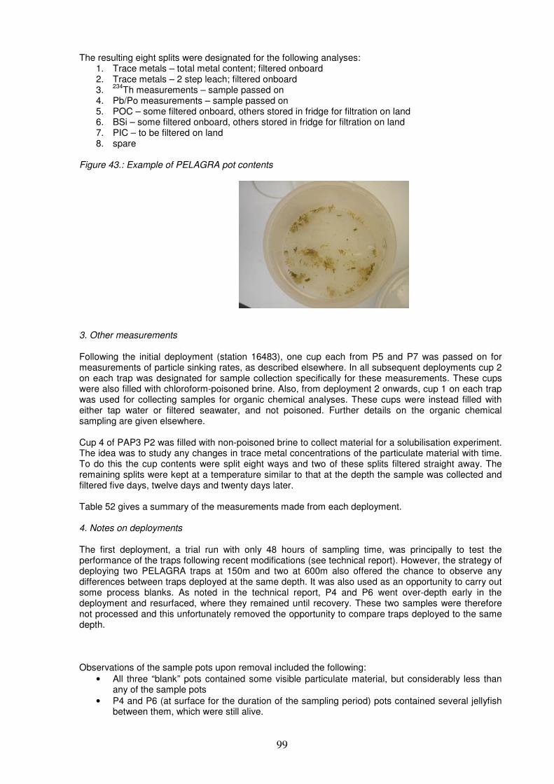
99
The resulting eight splits were designated for the following analyses: 1. Trace metals – total metal content; filtered onboard 2. Trace metals – 2 step leach; filtered onboard 3.
234Th measurements – sample passed on
4. Pb/Po measurements – sample passed on 5. POC – some filtered onboard, others stored in fridge for filtration on land 6. BSi – some filtered onboard, others stored in fridge for filtration on land 7. PIC – to be filtered on land 8. spare
Figure 43.: Example of PELAGRA pot contents
3. Other measurements Following the initial deployment (station 16483), one cup each from P5 and P7 was passed on for measurements of particle sinking rates, as described elsewhere. In all subsequent deployments cup 2 on each trap was designated for sample collection specifically for these measurements. These cups were also filled with chloroform-poisoned brine. Also, from deployment 2 onwards, cup 1 on each trap was used for collecting samples for organic chemical analyses. These cups were instead filled with either tap water or filtered seawater, and not poisoned. Further details on the organic chemical sampling are given elsewhere. Cup 4 of PAP3 P2 was filled with non-poisoned brine to collect material for a solubilisation experiment. The idea was to study any changes in trace metal concentrations of the particulate material with time. To do this the cup contents were split eight ways and two of these splits filtered straight away. The remaining splits were kept at a temperature similar to that at the depth the sample was collected and filtered five days, twelve days and twenty days later. Table 52 gives a summary of the measurements made from each deployment. 4. Notes on deployments The first deployment, a trial run with only 48 hours of sampling time, was principally to test the performance of the traps following recent modifications (see technical report). However, the strategy of deploying two PELAGRA traps at 150m and two at 600m also offered the chance to observe any differences between traps deployed at the same depth. It was also used as an opportunity to carry out some process blanks. As noted in the technical report, P4 and P6 went over-depth early in the deployment and resurfaced, where they remained until recovery. These two samples were therefore not processed and this unfortunately removed the opportunity to compare traps deployed to the same depth. Observations of the sample pots upon removal included the following:
• All three “blank” pots contained some visible particulate material, but considerably less than any of the sample pots
• P4 and P6 (at surface for the duration of the sampling period) pots contained several jellyfish between them, which were still alive.
100
• All sample pots contained particulate material consisting of fluffy green-brown aggregated material (marine snow) with varying numbers of dead swimmers of several species (see Figure 43). The presence of still-living jellyfish in P4 and P6 pots is ascribed partly to the possibility that the organisms entered the pots shortly before recovery and partly due to the chloroform being washed out of the pots due to greater wave action at the ocean surface.
The jellyfish observed in pots of P4 and P6 following deployment 1 were a common feature of deployments in the upper water column. Where jellyfish were found in the pots used for core measurements, they were removed with tweezers prior to combining pots. This unfortunately resulted in some particulate material also being lost, as it tended to stick to the jellyfish, but a record was kept of any time this was done. The third deployment had large numbers of other swimmers. Table 52. Summary of measurements made from PELAGRA deployments For the second and later deployments, all five PELAGRA traps were deployed at different depths. The target depths were: P2 – 50m, P4 – 150m, P5 – 300m, P6 – 450m, P7 – 600m. Although the target depths were not always reached (see technical report) samples were still processed except where the trap had been floating at the surface during collection (PAP1 P4 & P6, PAP3 P6).
PELAGRA deployment
Station Measurements made Notes
PAP1 P2 16483 Cups 1, 2, 3 – core measurements Cup 4 – process blank
Jellyfish
PAP1 P4 16483 Cups 1-3 – not processed Cup 4 – process blank
PAP1 P5 16483 Cups 1-3 – core measurements Cup 4 - particle sinking measurements
PAP1 P6 16483 Cups 1-3 – not processed Cup 4 – process blank
PAP1 P7 16483 Cups 1-3 – core measurements Cup 4 – particle sinking measurements
PAP2 P2 16515 Cup 1 – organic chemistry Cup 2 – particle sinking measurements Cups 3&4 – core measurements
Cup 2 partially dissolved by chloroform.
PAP2 P4 16516 Not processed PAP2 P5 16517 Cup 1 – organic chemistry
Cup 2 – particle sinking measurements Cups 3&4 – core measurements
Cup 2 partially dissolved by chloroform. Jellyfish in pot 1
PAP2 P6 16518 Cup 1 – organic chemistry Cup 2 – particle sinking measurements Cups 3&4 – core measurements
Cup 2 partially dissolved by chloroform.
PAP2 P7 16519 Cup 1 – organic chemistry Cup 2 – particle sinking measurements Cups 3&4 – core measurements
Cup 2 partially dissolved by chloroform.
PAP3 P2 16574 Cup 1 – organic chemistry Cup 2 – particle sinking measurements Cup 3 – core measurements Cup 4 – solubilisation experiment
Jellyfish in pots 1 & 2. Active swimmers in pot 4
PAP3 P4 16575 Cup 1 – organic chemistry Cup 2 – particle sinking measurements Cups 3&4 – core measurements
PAP3 P5 16576 Cup 1 – organic chemistry Cup 2 – particle sinking measurements Cups 3&4 – core measurements
Some active swimmers
PAP3 P6 16577 Not processed PAP3 P7 16578 Cup 1 – organic chemistry
Cup 2 – particle sinking measurements Cups 3&4 – core measurements
Large numbers of dead swimmers
PAP4 P2 16622 Cup 1 – organic chemistry Cup 2 – particle sinking measurements Cups 3&4 – core measurements
PAP4 P4 16623 Cup 1 – organic chemistry Cup 2 – particle sinking measurements Cups 3&4 – core measurements
PAP4 P5 16624 Cup 1 – organic chemistry Cup 2 – particle sinking measurements Cups 3&4 – core measurements
PAP4 P6 16625 Cup 1 – organic chemistry Cup 2 – particle sinking measurements Cups 3&4 – core measurements
PAP4 P7 16626 Cup 1 – organic chemistry Cup 2 – particle sinking measurements Cups 3&4 – core measurements
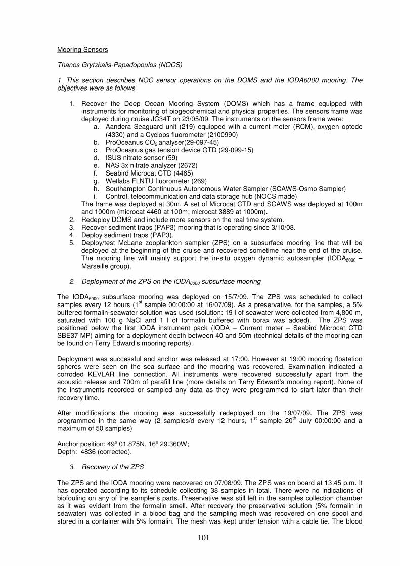
101
Mooring Sensors Thanos Grytzkalis-Papadopoulos (NOCS) 1. This section describes NOC sensor operations on the DOMS and the IODA6000 mooring. The objectives were as follows
1. Recover the Deep Ocean Mooring System (DOMS) which has a frame equipped with instruments for monitoring of biogeochemical and physical properties. The sensors frame was deployed during cruise JC34T on 23/05/09. The instruments on the sensors frame were:
a. Aandera Seaguard unit (219) equipped with a current meter (RCM), oxygen optode (4330) and a Cyclops fluorometer (2100990)
b. ProOceanus CO2 analyser(29-097-45) c. ProOceanus gas tension device GTD (29-099-15) d. ISUS nitrate sensor (59) e. NAS 3x nitrate analyzer (2672) f. Seabird Microcat CTD (4465) g. Wetlabs FLNTU fluorometer (269) h. Southampton Continuous Autonomous Water Sampler (SCAWS-Osmo Sampler) i. Control, telecommunication and data storage hub (NOCS made)
The frame was deployed at 30m. A set of Microcat CTD and SCAWS was deployed at 100m and 1000m (microcat 4460 at 100m; microcat 3889 at 1000m).
2. Redeploy DOMS and include more sensors on the real time system. 3. Recover sediment traps (PAP3) mooring that is operating since 3/10/08. 4. Deploy sediment traps (PAP3). 5. Deploy/test McLane zooplankton sampler (ZPS) on a subsurface mooring line that will be
deployed at the beginning of the cruise and recovered sometime near the end of the cruise. The mooring line will mainly support the in-situ oxygen dynamic autosampler (IODA6000 – Marseille group).
2. Deployment of the ZPS on the IODA6000 subsurface mooring
The IODA6000 subsurface mooring was deployed on 15/7/09. The ZPS was scheduled to collect samples every 12 hours (1
st sample 00:00:00 at 16/07/09). As a preservative, for the samples, a 5%
buffered formalin-seawater solution was used (solution: 19 l of seawater were collected from 4,800 m, saturated with 100 g NaCl and 1 l of formalin buffered with borax was added). The ZPS was positioned below the first IODA instrument pack (IODA – Current meter – Seabird Microcat CTD SBE37 MP) aiming for a deployment depth between 40 and 50m (technical details of the mooring can be found on Terry Edward’s mooring reports). Deployment was successful and anchor was released at 17:00. However at 19:00 mooring floatation spheres were seen on the sea surface and the mooring was recovered. Examination indicated a corroded KEVLAR line connection. All instruments were recovered successfully apart from the acoustic release and 700m of parafill line (more details on Terry Edward’s mooring report). None of the instruments recorded or sampled any data as they were programmed to start later than their recovery time. After modifications the mooring was successfully redeployed on the 19/07/09. The ZPS was programmed in the same way (2 samples/d every 12 hours, 1
st sample 20
th July 00:00:00 and a
maximum of 50 samples) Anchor position: 49º 01.875N, 16º 29.360W; Depth: 4836 (corrected).
3. Recovery of the ZPS
The ZPS and the IODA mooring were recovered on 07/08/09. The ZPS was on board at 13:45 p.m. It has operated according to its schedule collecting 38 samples in total. There were no indications of biofouling on any of the sampler’s parts. Preservative was still left in the samples collection chamber as it was evident from the formalin smell. After recovery the preservative solution (5% formalin in seawater) was collected in a blood bag and the sampling mesh was recovered on one spool and stored in a container with 5% formalin. The mesh was kept under tension with a cable tie. The blood
102
bag and the samples container were stored at 4 0C. The ZPS depth during deployment is presented in
figure 44. Figure 44: ZPS deployment depth during D341
4. Sediment traps subsurface moorings – PAP3 The PAP3 sediment traps mooring was deployed on 18/07/09. The sediment trap bottles were filled with 5% buffered formalin seawater one day before deployment. The deployment depths were as follows: Trap LVII-A (S.Nr. 12432-05) and current meter RCM8 at 3000 m Trap LVII-B (S. Nr. 12432-04) at 3000 m Trap LVII-C (S. Nr. 12432-06) and current meter RCM8 at 100 m above sea bed. Detailed sampling schedules of the sediment traps are on file D341 Sediment traps deployment schedule.xls. The current meters were set to record data every hour. The deployment details are: Latitude: 48
0 59.59’ N
Longitude: 160 29.21’W
Depth : 4810m (u); 4844 m (c). 5. PAP3 Recovery PAP3 (LIV deployment) mooring was recovered on 29/07/09. The mooring was released at 14:58 pm and the last sediment trap was on board at 17:46 pm. The sediment traps were: Trap LIV-A (S.Nr. 12168-01) and current meter RCM11 at 3000 m Trap LIV-B (S. Nr. 11262-03) at 3000 m Trap LIV-C (S. Nr. 11262-04) and current meter RCM11 at 100 m above sea bed. All sediment traps worked according to their schedule. The carousel was at position 21 in all traps (still sampling). All sampling bottles were recovered, pH was measured and 1 ml of buffered formalin was added. Samples were stored at 4
0C. The recovery files and sampling schedules were successfully
downloaded from all three sediment traps.
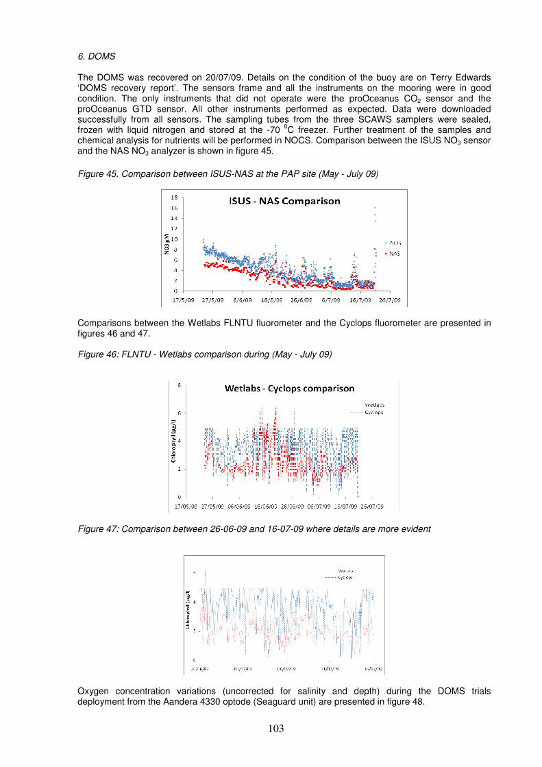
103
6. DOMS The DOMS was recovered on 20/07/09. Details on the condition of the buoy are on Terry Edwards ‘DOMS recovery report’. The sensors frame and all the instruments on the mooring were in good condition. The only instruments that did not operate were the proOceanus CO2 sensor and the proOceanus GTD sensor. All other instruments performed as expected. Data were downloaded successfully from all sensors. The sampling tubes from the three SCAWS samplers were sealed, frozen with liquid nitrogen and stored at the -70
0C freezer. Further treatment of the samples and
chemical analysis for nutrients will be performed in NOCS. Comparison between the ISUS NO3 sensor and the NAS NO3 analyzer is shown in figure 45.
Figure 45. Comparison between ISUS-NAS at the PAP site (May - July 09)
Comparisons between the Wetlabs FLNTU fluorometer and the Cyclops fluorometer are presented in figures 46 and 47. Figure 46: FLNTU - Wetlabs comparison during (May - July 09)
Figure 47: Comparison between 26-06-09 and 16-07-09 where details are more evident
Oxygen concentration variations (uncorrected for salinity and depth) during the DOMS trials deployment from the Aandera 4330 optode (Seaguard unit) are presented in figure 48.
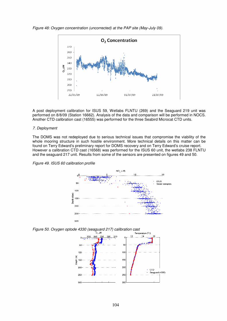
104
Figure 48: Oxygen concentration (uncorrected) at the PAP site (May-July 09).
A post deployment calibration for ISUS 59, Wetlabs FLNTU (269) and the Seaguard 219 unit was performed on 8/8/09 (Station 16662). Analysis of the data and comparison will be performed in NOCS. Another CTD calibration cast (16555) was performed for the three Seabird Microcat CTD units. 7. Deployment The DOMS was not redeployed due to serious technical issues that compromise the viability of the whole mooring structure in such hostile environment. More technical details on this matter can be found on Terry Edward’s preliminary report for DOMS recovery and on Terry Edward’s cruise report. However a calibration CTD cast (16568) was performed for the ISUS 60 unit, the wetlabs 238 FLNTU and the seaguard 217 unit. Results from some of the sensors are presented on figures 49 and 50. Figure 49. ISUS 60 calibration profile
Figure 50. Oxygen optode 4330 (seaguard 217) calibration cast
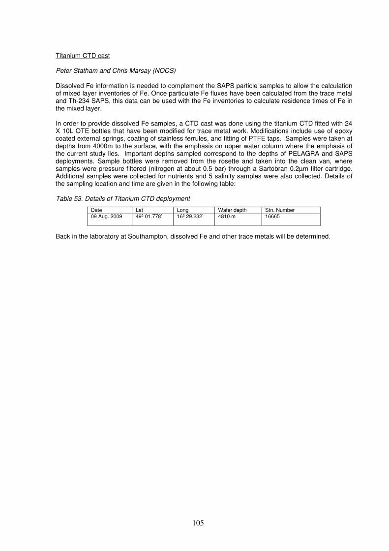
105
Titanium CTD cast Peter Statham and Chris Marsay (NOCS) Dissolved Fe information is needed to complement the SAPS particle samples to allow the calculation of mixed layer inventories of Fe. Once particulate Fe fluxes have been calculated from the trace metal and Th-234 SAPS, this data can be used with the Fe inventories to calculate residence times of Fe in the mixed layer. In order to provide dissolved Fe samples, a CTD cast was done using the titanium CTD fitted with 24 X 10L OTE bottles that have been modified for trace metal work. Modifications include use of epoxy coated external springs, coating of stainless ferrules, and fitting of PTFE taps. Samples were taken at depths from 4000m to the surface, with the emphasis on upper water column where the emphasis of the current study lies. Important depths sampled correspond to the depths of PELAGRA and SAPS deployments. Sample bottles were removed from the rosette and taken into the clean van, where samples were pressure filtered (nitrogen at about 0.5 bar) through a Sartobran 0.2µm filter cartridge. Additional samples were collected for nutrients and 5 salinity samples were also collected. Details of the sampling location and time are given in the following table: Table 53. Details of Titanium CTD deployment Back in the laboratory at Southampton, dissolved Fe and other trace metals will be determined.
Date Lat Long Water depth Stn. Number 09 Aug. 2009
49º 01.778’ 16º 29.232’ 4810 m 16665
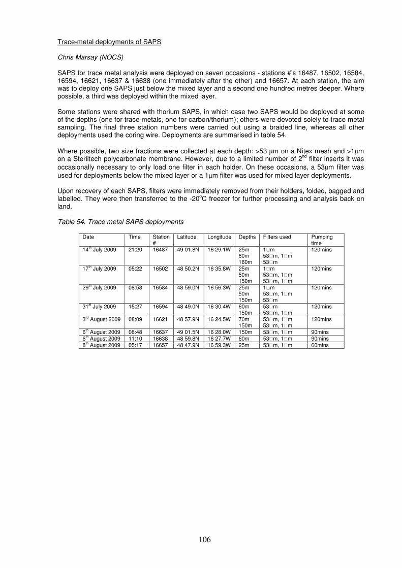
106
Trace-metal deployments of SAPS Chris Marsay (NOCS) SAPS for trace metal analysis were deployed on seven occasions - stations #’s 16487, 16502, 16584, 16594, 16621, 16637 & 16638 (one immediately after the other) and 16657. At each station, the aim was to deploy one SAPS just below the mixed layer and a second one hundred metres deeper. Where possible, a third was deployed within the mixed layer. Some stations were shared with thorium SAPS, in which case two SAPS would be deployed at some of the depths (one for trace metals, one for carbon/thorium); others were devoted solely to trace metal sampling. The final three station numbers were carried out using a braided line, whereas all other deployments used the coring wire. Deployments are summarised in table 54.
Where possible, two size fractions were collected at each depth: >53 µm on a Nitex mesh and >1µm on a Sterlitech polycarbonate membrane. However, due to a limited number of 2
nd filter inserts it was
occasionally necessary to only load one filter in each holder. On these occasions, a 53µm filter was
used for deployments below the mixed layer or a 1µm filter was used for mixed layer deployments. Upon recovery of each SAPS, filters were immediately removed from their holders, folded, bagged and labelled. They were then transferred to the -20
oC freezer for further processing and analysis back on
land. Table 54. Trace metal SAPS deployments
Date Time Station #
Latitude Longitude Depths Filters used Pumping time
14th July 2009 21:20 16487 49 01.8N 16 29.1W 25m
60m 160m
1m 53m, 1m 53m
120mins
17th July 2009 05:22 16502 48 50.2N 16 35.8W 25m
50m 150m
1m 53m, 1m 53m, 1m
120mins
29th July 2009 08:58 16584 48 59.0N 16 56.3W 25m
50m 150m
1m 53m, 1m 53m
120mins
31st July 2009 15:27 16594 48 49.0N 16 30.4W 60m
150m 53m 53m, 1m
120mins
3rd August 2009 08:09 16621 48 57.9N 16 24.5W 70m
150m 53m, 1m 53m, 1m
120mins
6th August 2009 08:48 16637 49 01.5N 16 28.0W 150m 53m, 1m 90mins
6th August 2009 11:10 16638 48 59.8N 16 27.7W 60m 53m, 1m 90mins
8th August 2009 05:17 16657 48 47.9N 16 59.3W 25m 53m, 1m 60mins
107
Oxygen consumption and evolution Dominique Lefèvre & Anne Robert (LMGEM)
1. Objectives The objective of the work was to measure biological fluxes of oxygen throughout the water column. Dissolved oxygen was determined via the Winkler method with a photometric detection of endpoint value (Williams & Jenkinson, 1982). In situ oxygen consumption and evolution rates were determined using the IODA6000 (In situ Oxygen Dynamics Autosampler) autosampler developed by the LMGEM in collaboration with the CPPM (Centre de Physique des Particules de Marseille). Electron Transport System (ETS) Enzymatic determination of bacterial respiration was determined by measurement of Electron Transport System (ETS) with spectrophotometric determination (Packard, 1971). 2. Sampling strategy 1743 oxygen samples were analysed during the cruise. A daily calibration of the thiosulfate was performed and cross calibration was performed using reference standard KIO3 (Osil, Iodate standard) at the beginning and end of the cruise, 75 ETS samples for 6 vertical profiles up to 2000m depth were collected. A mooring including 5 IODA6000, 4 MicroCAT and 3 Aquadopp was deployed over 20 days Vertical profiles of net community production were undertaken at 6 depths corresponding to 55%, 33%, 14%, 7%, 3% and 1% of surface PAR at 8 stations (D16524, 16533, 16543, 16552, 16567, 16580, 16635, 16655) for deck incubation and 8 depths (55%, 33%, 20%, 15%, 7%, 3%, 1% and 0.1% of PAR) at 3 stations (D16488, 16501 and 16597) for incubation on a drifter mooring line. The Vertical distribution of dissolved O2 was measured at 23 stations to calibrate the SBE 43 sensor and to characterise the environment of the fixed moorings (i.e. PAP3, French mooring line) Microbial respiration rates in euphotic layer was measured at 2 stations using seawater filtered at 0.6µm using an inverse filtration system. Microbial respiration rates in meso and bathypelagic layers were measured at 4 depths (150, 500, 1000m and 2000 m) at 8 stations (16488, 16489, 16591, 16619 and 16659). Vertical ETS profiles were carried out, with 13 depths sampled between 5 m and 2000m. 3. Analysis and post-cruise processing, time required for full processing/analysis. Oxygen analysies were performed on board, Validated data will be made available at the end of2009. ETS samples are stored in liquid nitrogen and should be analysed in 2010. Validated data will be made available at the end 2010, IODA6000, CTD-Seabird-microcat® and Current-meter-Aquadopp® data will be processed for mid 2010. 3. Error and accuracy Accuracy of dissolved oxygen concentration determination for vertical profiles: 0.05 µmol dm
-3
Accuracy of the biological fluxes of dissolved oxygen by Winkler method : 0.2 µmol O2 dm-3
d-1
Accuracy of the biological fluxes of dissolved oxygen using the IODA6000 0.4 µmol O2 dm
-3 d
-1
(unpublished data) Accuracy of ETS activity (0.001 µmol O2 dm
-3 h
-1, Lefevre et al., 1996).
4. References WILLIAMS P.J. LEB. & N.W. JENKINSON (1982). A transportable microprocessor-controlled precise Winkler titration suitable for field station and shipboard use. Limnol. Oceanogr. 27, 576-585. Packard, T.T., 1971. The measurement of respiratory electron-electron-transport activity in marine phytoplankton. J. Mar.Res., 29: 235-244. Lefèvre, D., M. Denis, C.E. Lambert, J.-C. Miquel, 1996. Is DOC the main source of organic matter remineralisation in the ocean water column? ’Journal of Marine Systems 7 (1996) 281-291