9 overcurrent protection for phase and earth faults - · pdf file• 9 • overcurrent...
TRANSCRIPT
Introduction 9.1
Co-ordination procedure 9.2
Principles of time/current grading 9.3
Standard I.D.M.T. overcurrent relays 9.4
Combined I.D.M.T. and high set instantaneous overcurrent relays 9.5
Very Inverse overcurrent relays 9.6
Extremely Inverse overcurrent relays 9.7
Other relay characteristics 9.8
Independent (definite) time overcurrent relays 9.9
Relay current setting 9.10
Relay time grading margin 9.11
Recommended grading margins 9.12
Calculation of phase fault overcurrent relay settings 9.13
Directional phase fault overcurrent relays 9.14
Ring mains 9.15
Earth fault protection 9.16
Directional earth fault overcurrent protection 9.17
Earth fault protection on insulated networks 9.18
Earth fault protection on Petersen Coil earthed networks 9.19
Examples of time and current grading 9.20
References 9.21
• 9 • O v e r c u r r e n t P r o t e c t i o n f o r P h a s e a n d E a r t h F a u l t s
N e t w o r k P r o t e c t i o n & A u t o m a t i o n G u i d e • 1 2 3 •
9.1 INTRODUCTION
Protection against excess current was naturally theearliest protection system to evolve. From this basicprinciple, the graded overcurrent system, a discriminativefault protection, has been developed. This should not beconfused with ‘overload’ protection, which normallymakes use of relays that operate in a time related insome degree to the thermal capability of the plant to beprotected. Overcurrent protection, on the other hand, isdirected entirely to the clearance of faults, although withthe settings usually adopted some measure of overloadprotection may be obtained.
9.2 CO-ORDINATION PROCEDURE
Correct overcurrent relay application requires knowledgeof the fault current that can flow in each part of thenetwork. Since large-scale tests are normallyimpracticable, system analysis must be used – seeChapter 4 for details. The data required for a relaysetting study are:
i. a one-line diagram of the power system involved,showing the type and rating of the protectiondevices and their associated current transformers
ii. the impedances in ohms, per cent or per unit, ofall power transformers, rotating machine andfeeder circuits
iii. the maximum and minimum values of short circuitcurrents that are expected to flow through eachprotection device
iv. the maximum load current through protectiondevices
v. the starting current requirements of motors andthe starting and locked rotor/stalling times ofinduction motors
vi. the transformer inrush, thermal withstand anddamage characteristics
vii. decrement curves showing the rate of decay ofthe fault current supplied by the generators
viii. performance curves of the current transformers
The relay settings are first determined to give theshortest operating times at maximum fault levels and
• 9 • O ve r c u r re n t P ro te c t i o n for Phase and Ear th Faults
N e t w o r k P r o t e c t i o n & A u t o m a t i o n G u i d e
• 9 •
Ove
rcur
rent
Pro
tect
ion
for
Phas
e an
d E
arth
Fau
lts
• 1 2 4 •
then checked to see if operation will also be satisfactoryat the minimum fault current expected. It is alwaysadvisable to plot the curves of relays and otherprotection devices, such as fuses, that are to operate inseries, on a common scale. It is usually more convenientto use a scale corresponding to the current expected atthe lowest voltage base, or to use the predominantvoltage base. The alternatives are a common MVA baseor a separate current scale for each system voltage.
The basic rules for correct relay co-ordination can generallybe stated as follows:
a. whenever possible, use relays with the sameoperating characteristic in series with each other
b. make sure that the relay farthest from the sourcehas current settings equal to or less than the relaysbehind it, that is, that the primary current requiredto operate the relay in front is always equal to orless than the primary current required to operatethe relay behind it.
9.3 PRINCIPLES OF TIME/CURRENT GRADING
Among the various possible methods used to achievecorrect relay co-ordination are those using either time orovercurrent, or a combination of both. The common aimof all three methods is to give correct discrimination.That is to say, each one must isolate only the faultysection of the power system network, leaving the rest ofthe system undisturbed.
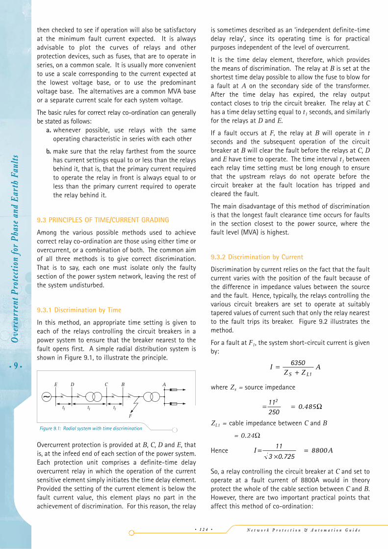
9.3.1 Discrimination by Time
In this method, an appropriate time setting is given toeach of the relays controlling the circuit breakers in apower system to ensure that the breaker nearest to thefault opens first. A simple radial distribution system isshown in Figure 9.1, to illustrate the principle.
Overcurrent protection is provided at B, C, D and E, thatis, at the infeed end of each section of the power system.Each protection unit comprises a definite-time delayovercurrent relay in which the operation of the currentsensitive element simply initiates the time delay element.Provided the setting of the current element is below thefault current value, this element plays no part in theachievement of discrimination. For this reason, the relay
is sometimes described as an ‘independent definite-timedelay relay’, since its operating time is for practicalpurposes independent of the level of overcurrent.
It is the time delay element, therefore, which providesthe means of discrimination. The relay at B is set at theshortest time delay possible to allow the fuse to blow fora fault at A on the secondary side of the transformer.After the time delay has expired, the relay outputcontact closes to trip the circuit breaker. The relay at Chas a time delay setting equal to t1 seconds, and similarlyfor the relays at D and E.
If a fault occurs at F, the relay at B will operate in tseconds and the subsequent operation of the circuitbreaker at B will clear the fault before the relays at C, Dand E have time to operate. The time interval t1 betweeneach relay time setting must be long enough to ensurethat the upstream relays do not operate before thecircuit breaker at the fault location has tripped andcleared the fault.
The main disadvantage of this method of discriminationis that the longest fault clearance time occurs for faultsin the section closest to the power source, where thefault level (MVA) is highest.
9.3.2 Discrimination by Current
Discrimination by current relies on the fact that the faultcurrent varies with the position of the fault because ofthe difference in impedance values between the sourceand the fault. Hence, typically, the relays controlling thevarious circuit breakers are set to operate at suitablytapered values of current such that only the relay nearestto the fault trips its breaker. Figure 9.2 illustrates themethod.
For a fault at F1, the system short-circuit current is givenby:
where Zs = source impedance
ZL1 = cable impedance between C and B
= 0.24Ω
Hence
So, a relay controlling the circuit breaker at C and set tooperate at a fault current of 8800A would in theoryprotect the whole of the cable section between C and B.However, there are two important practical points thataffect this method of co-ordination:
I A=×
=113 0 725.
8800
= =11250
2 0.485Ω
IZ Z
AS L
=+
6350
1
Figure 9.1: Radial system with time discrimination
t1F
DE
t1 t1
C B A

N e t w o r k P r o t e c t i o n & A u t o m a t i o n G u i d e • 1 2 5 •
• 9 •O
verc
urre
nt P
rote
ctio
n fo
r Ph
ase
and
Ear
th F
aults
a. it is not practical to distinguish between a fault atF1 and a fault at F2, since the distance betweenthese points may be only a few metres,corresponding to a change in fault current ofapproximately 0.1%
b. in practice, there would be variations in the sourcefault level, typically from 250MVA to 130MVA. Atthis lower fault level the fault current would notexceed 6800A, even for a cable fault close to C. Arelay set at 8800A would not protect any part ofthe cable section concerned
Discrimination by current is therefore not a practicalproposition for correct grading between the circuitbreakers at C and B. However, the problem changesappreciably when there is significant impedancebetween the two circuit breakers concerned. Considerthe grading required between the circuit breakers at Cand A in Figure 9.2. Assuming a fault at F4, the short-circuit current is given by:
where ZS = source impedance
= 0.485Ω
ZL1 = cable impedance between C and B
= 0.24Ω
ZL2 = cable impedance between B and 4 MVAtransformer
= 0.04Ω
ZT = transformer impedance
= 2.12Ω
Hence
= 2200 A
For this reason, a relay controlling the circuit breaker atB and set to operate at a current of 2200A plus a safetymargin would not operate for a fault at F4 and wouldthus discriminate with the relay at A. Assuming a safety
I =×11
3 2 885.
= ⎛⎝⎜
⎞⎠⎟
0 07 114
2.
IZ Z
AS L
=+
6350
1
margin of 20% to allow for relay errors and a further10% for variations in the system impedance values, it isreasonable to choose a relay setting of 1.3 x 2200A, thatis 2860A, for the relay at B. Now, assuming a fault at F3,at the end of the 11kV cable feeding the 4MVAtransformer, the short-circuit current is given by:
Thus, assuming a 250MVA source fault level:
= 8300 A
Alternatively, assuming a source fault level of 130MVA:
= 5250 A
In other words, for either value of source level, the relayat B would operate correctly for faults anywhere on the11kV cable feeding the transformer.
9.3.3 Discrimination by both Time and Current
Each of the two methods described so far has afundamental disadvantage. In the case of discriminationby time alone, the disadvantage is due to the fact thatthe more severe faults are cleared in the longestoperating time. On the other hand, discrimination bycurrent can be applied only where there is appreciableimpedance between the two circuit breakers concerned.
It is because of the limitations imposed by theindependent use of either time or current co-ordinationthat the inverse time overcurrent relay characteristic hasevolved. With this characteristic, the time of operationis inversely proportional to the fault current level and theactual characteristic is a function of both ‘time’and 'current' settings. Figure 9.3 illustrates thecharacteristics of two relays given different current/timesettings. For a large variation in fault current betweenthe two ends of the feeder, faster operating times can beachieved by the relays nearest to the source, where thefault level is the highest. The disadvantages of gradingby time or current alone are overcome.
The selection of overcurrent relay characteristicsgenerally starts with selection of the correctcharacteristic to be used for each relay, followed bychoice of the relay current settings. Finally the gradingmargins and hence time settings of the relays aredetermined. An iterative procedure is often required toresolve conflicts, and may involve use of non-optimalcharacteristics, current or time grading settings.
I =+ +( )11
3 0 93 0 214 0 04 . . .
I =+ +( )11
3 0 485 0 24 0 04 . . .
IZ Z ZS L L
=+ +( )11
3 1 2
CF1 F3F2 F4
B A
11kV250MVASource
200 metres240mm2 P.I.L.C.
Cable
200 metres240mm2 P.I.L.C.
Cable
4MVA11/3.3kV
7%
Figure 9.2: Radial system with current discrimination
N e t w o r k P r o t e c t i o n & A u t o m a t i o n G u i d e
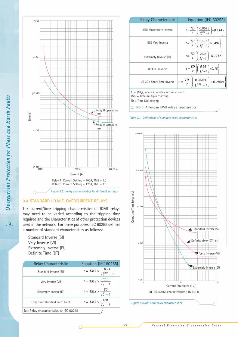
9.4 STANDARD I.D.M.T. OVERCURRENT RELAYS
The current/time tripping characteristics of IDMT relaysmay need to be varied according to the tripping timerequired and the characteristics of other protection devicesused in the network. For these purposes, IEC 60255 definesa number of standard characteristics as follows:
Standard Inverse (SI)Very Inverse (VI)Extremely Inverse (EI)Definite Time (DT)
• 9 •
Ove
rcur
rent
Pro
tect
ion
for
Phas
e an
d E
arth
Fau
lts
• 1 2 6 •
Figure 9.3: Relay characteristics for different settings
1000.10
1.00
Relay A: Current Setting = 100A, TMS = 1.0
1000 10,000
time
Relay A operatingtime
10.00
100.
1000.
Relay B: Current Setting = 125A, TMS = 1.3
Current (A)
Tim
e (s
)
Table 9.1: Definitions of standard relay characteristics
Figure 9.4 (a): IDMT relay characteristics
(a) IEC 60255 characteristics ; TMS=1.0
Ope
ratin
g Ti
me
(sec
onds
)
Current (multiples of ISI )
0.1010
1.00
10.00
100.00
1000.00
1001
Ir = (I/Is), where Is = relay setting currentTMS = Time multiplier Setting
TD = Time Dial setting
(b): North American IDMT relay characteristics
Relay Characteristic Equation (IEC 60255)
IEEE Moderately Inverse
IEEE Very Inverse
Extremely Inverse (EI)
US CO8 Inverse
US CO2 Short Time Inverse t TD
I=
−
⎛
⎝⎜
⎞
⎠⎟ +
⎧⎨⎪
⎩⎪
⎫⎬⎪
⎭⎪70 02394
10 01694
0 02
. ..
r
t TDIr
=−
⎛⎝⎜
⎞⎠⎟
+⎧⎨⎩
⎫⎬⎭7
5 951
0 182
. .
t TDIr
=−
⎛⎝⎜
⎞⎠⎟
+⎧⎨⎩
⎫⎬⎭7
28 21
0 12172
. .
t TDIr
=−
⎛⎝⎜
⎞⎠⎟
+⎧⎨⎩
⎫⎬⎭7
19 611
0 4912
. .
t TDIr
=−
⎛⎝⎜
⎞⎠⎟
+⎧⎨⎩
⎫⎬⎭7
0 05151
0 1140 02
. ..
Relay Characteristic Equation (IEC 60255)
Standard Inverse (SI)
Very Inverse (VI)
Extremely Inverse (EI)
Long time standard earth fault t TMSI r
= ×−
1201
t TMSI r
= ×−
8012
t TMSI r
= ×−
13 51
.
t TMSI r
= ×−
0 1410 02
..
(a): Relay characteristics to IEC 60255

N e t w o r k P r o t e c t i o n & A u t o m a t i o n G u i d e • 1 2 7 •
The mathematical descriptions of the curves are given inTable 9.1(a), and the curves based on a common settingcurrent and time multiplier setting of 1 second areshown in Figure 9.4(a). The tripping characteristics fordifferent TMS settings using the SI curve are illustratedin Figure 9.5.
Although the curves are only shown for discrete values ofTMS, continuous adjustment may be possible in anelectromechanical relay. For other relay types, the settingsteps may be so small as to effectively provide continuousadjustment. In addition, almost all overcurrent relays arealso fitted with a high-set instantaneous element.
In most cases, use of the standard SI curve provessatisfactory, but if satisfactory grading cannot beachieved, use of the VI or EI curves may help to resolvethe problem. When digital or numeric relays are used,other characteristics may be provided, including thepossibility of user-definable curves. More details areprovided in the following sections.
Relays for power systems designed to North Americanpractice utilise ANSI/IEEE curves. Table 9.1(b) gives themathematical description of these characteristics andFigure 9.4(b) shows the curves standardised to a timedial setting of 1.0.
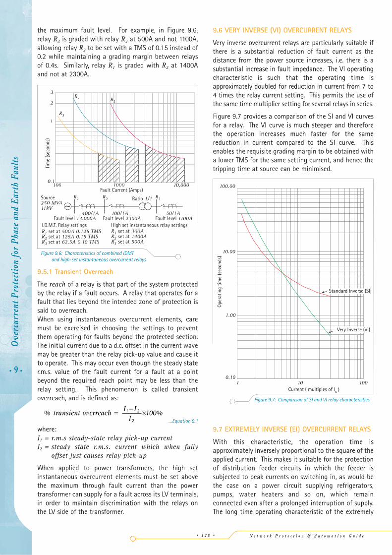
9.5 COMBINED I.D.M.T. AND HIGH SET INSTANTANEOUS OVERCURRENT RELAYS
A high-set instantaneous element can be used where thesource impedance is small in comparison with theprotected circuit impedance. This makes a reduction inthe tripping time at high fault levels possible. It alsoimproves the overall system grading by allowing the'discriminating curves' behind the high set instantaneouselements to be lowered.
As shown in Figure 9.6, one of the advantages of the highset instantaneous elements is to reduce the operatingtime of the circuit protection by the shaded area belowthe 'discriminating curves'. If the source impedanceremains constant, it is then possible to achieve high-speed protection over a large section of the protectedcircuit. The rapid fault clearance time achieved helps tominimise damage at the fault location. Figure 9.6 alsoillustrates a further important advantage gained by theuse of high set instantaneous elements. Grading withthe relay immediately behind the relay that has theinstantaneous elements enabled is carried out at thecurrent setting of the instantaneous elements and not at
• 9 •O
verc
urre
nt P
rote
ctio
n fo
r Ph
ase
and
Ear
th F
aults
Figure 9.5: Typical time/current characteristics of standard IDMT relay
Tim
e (s
econ
ds)
Current (multiples of plug settings)
2
3
4
6
8
10
1
2 3 4 6 8 10 20 3010.1
0.2
0.4
0.3
0.6
0.8
1.0TMS
0.90.80.70.60.5
0.4
0.3
0.2
0.1
Figure 9.4 (b): IDMT relay characteristics
(b) North American characteristics; TD=7
0.10101
1.00
10.00
100.00
1000.00
100
Ope
ratin
g Ti
me
(sec
onds
)
Current (multiples of ISI )
Moderately Inverse
Time Inverse
CO 8 Inverse
ExtremelyInverse
N e t w o r k P r o t e c t i o n & A u t o m a t i o n G u i d e
the maximum fault level. For example, in Figure 9.6,relay R2 is graded with relay R3 at 500A and not 1100A,allowing relay R2 to be set with a TMS of 0.15 instead of0.2 while maintaining a grading margin between relaysof 0.4s. Similarly, relay R1 is graded with R2 at 1400Aand not at 2300A.
9.5.1 Transient Overreach
The reach of a relay is that part of the system protectedby the relay if a fault occurs. A relay that operates for afault that lies beyond the intended zone of protection issaid to overreach.When using instantaneous overcurrent elements, caremust be exercised in choosing the settings to preventthem operating for faults beyond the protected section.The initial current due to a d.c. offset in the current wavemay be greater than the relay pick-up value and cause itto operate. This may occur even though the steady stater.m.s. value of the fault current for a fault at a pointbeyond the required reach point may be less than therelay setting. This phenomenon is called transientoverreach, and is defined as:
…Equation 9.1
where:I1 = r.m.s steady-state relay pick-up currentI2 = steady state r.m.s. current which when fully
offset just causes relay pick-up
When applied to power transformers, the high setinstantaneous overcurrent elements must be set abovethe maximum through fault current than the powertransformer can supply for a fault across its LV terminals,in order to maintain discrimination with the relays onthe LV side of the transformer.
% % transient overreach = − ×I II
1 2
2100
9.6 VERY INVERSE (VI) OVERCURRENT RELAYS
Very inverse overcurrent relays are particularly suitable ifthere is a substantial reduction of fault current as thedistance from the power source increases, i.e. there is asubstantial increase in fault impedance. The VI operatingcharacteristic is such that the operating time isapproximately doubled for reduction in current from 7 to4 times the relay current setting. This permits the use ofthe same time multiplier setting for several relays in series.
Figure 9.7 provides a comparison of the SI and VI curvesfor a relay. The VI curve is much steeper and thereforethe operation increases much faster for the samereduction in current compared to the SI curve. Thisenables the requisite grading margin to be obtained witha lower TMS for the same setting current, and hence thetripping time at source can be minimised.
9.7 EXTREMELY INVERSE (EI) OVERCURRENT RELAYS
With this characteristic, the operation time isapproximately inversely proportional to the square of theapplied current. This makes it suitable for the protectionof distribution feeder circuits in which the feeder issubjected to peak currents on switching in, as would bethe case on a power circuit supplying refrigerators,pumps, water heaters and so on, which remainconnected even after a prolonged interruption of supply.The long time operating characteristic of the extremely
• 9 •
Ove
rcur
rent
Pro
tect
ion
for
Phas
e an
d E
arth
Fau
lts
• 1 2 8 •
Ope
ratin
g tim
e (s
econ
ds)
0.10101
1.00
10.00
100.00
100Current ( multiples of Is )
Standard Inverse (SI)
Very Inverse (VI)
Figure 9.7: Comparison of SI and VI relay characteristics
Figure 9.6: Characteristics of combined IDMT and high-set instantaneous overcurrent relays
Tim
e (s
econ
ds)
2
3
1
100001000.1
400/1A
R1 R2 R3Source250 MVA11kV
100/1A 50/1AFault level 13.000A Fault level 2300A Fault level 1100A
Ratio
10,0000
R3
R2 RR1
500A 0.125 TMS
62.5A 0.10 TMS
300A
500A

N e t w o r k P r o t e c t i o n & A u t o m a t i o n G u i d e • 1 2 9 •
inverse relay at normal peak load values of current alsomakes this relay particularly suitable for grading withfuses. Figure 9.8 shows typical curves to illustrate this.It can be seen that use of the EI characteristic gives asatisfactory grading margin, but use of the VI or SIcharacteristics at the same settings does not. Anotherapplication of this relay is in conjunction with auto-reclosers in low voltage distribution circuits. Themajority of faults are transient in nature andunnecessary blowing and replacing of the fuses presentin final circuits of such a system can be avoided if theauto-reclosers are set to operate before the fuse blows.If the fault persists, the auto-recloser locks itself in theclosed position after one opening and the fuse blows toisolate the fault.
9.8 OTHER RELAY CHARACTERISTICS
User definable curves may be provided on some types ofdigital or numerical relays. The general principle is that theuser enters a series of current/time co-ordinates that arestored in the memory of the relay. Interpolation betweenpoints is used to provide a smooth trip characteristic. Sucha feature, if available, may be used in special cases if noneof the standard tripping characteristics is suitable.However, grading of upstream protection may becomemore difficult, and it is necessary to ensure that the curve
is properly documented, along with the reasons for use.Since the standard curves provided cover most cases withadequate tripping times, and most equipment is designedwith standard protection curves in mind, the need to utilisethis form of protection is relatively rare.
Digital and numerical relays may also include pre-defined logic schemes utilising digital (relay) I/Oprovided in the relay to implement standard schemessuch as CB failure and trip circuit supervision. This savesthe provision of separate relay or PLC (ProgrammableLogic Controller) hardware to perform these functions.
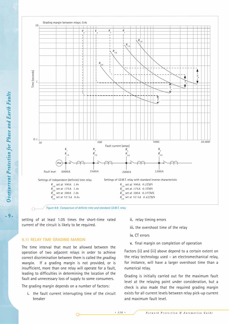
9.9 INDEPENDENT (DEFINITE) TIMEOVERCURRENT RELAYS
Overcurrent relays are normally also provided withelements having independent or definite timecharacteristics. These characteristics provide a readymeans of co-ordinating several relays in series insituations in which the system fault current varies verywidely due to changes in source impedance, as there isno change in time with the variation of fault current.The time/current characteristics of this curve are shownin Figure 9.9, together with those of the standard I.D.M.T.characteristic, to indicate that lower operating times areachieved by the inverse relay at the higher values of faultcurrent, whereas the definite time relay has loweroperating times at the lower current values.
Vertical lines T1, T2, T3, and T4 indicate the reduction inoperating times achieved by the inverse relay at highfault levels.
9.10 RELAY CURRENT SETTING
An overcurrent relay has a minimum operating current,known as the current setting of the relay. The currentsetting must be chosen so that the relay does notoperate for the maximum load current in the circuitbeing protected, but does operate for a current equal orgreater to the minimum expected fault current.Although by using a current setting that is only justabove the maximum load current in the circuit a certaindegree of protection against overloads as well as faultsmay be provided, the main function of overcurrentprotection is to isolate primary system faults and not toprovide overload protection. In general, the currentsetting will be selected to be above the maximum shorttime rated current of the circuit involved. Since all relayshave hysteresis in their current settings, the setting mustbe sufficiently high to allow the relay to reset when therated current of the circuit is being carried. The amountof hysteresis in the current setting is denoted by thepick-up/drop-off ratio of a relay – the value for a modernrelay is typically 0.95. Thus, a relay minimum current
• 9 •O
verc
urre
nt P
rote
ctio
n fo
r Ph
ase
and
Ear
th F
aults
Figure 9.8: Comparison of relay and fuse characteristics
1000.1
1000
1.0
10.0
100.0
10,000
200.0
Standardinverse (SI)
Current (amps)
Tim
e (s
ecs)
inverse (EI) Es E
200A Fuseus
v
A
N e t w o r k P r o t e c t i o n & A u t o m a t i o n G u i d e
setting of at least 1.05 times the short-time ratedcurrent of the circuit is likely to be required.
9.11 RELAY TIME GRADING MARGIN
The time interval that must be allowed between theoperation of two adjacent relays in order to achievecorrect discrimination between them is called the gradingmargin. If a grading margin is not provided, or isinsufficient, more than one relay will operate for a fault,leading to difficulties in determining the location of thefault and unnecessary loss of supply to some consumers.
The grading margin depends on a number of factors:
i. the fault current interrupting time of the circuitbreaker
ii. relay timing errors
iii. the overshoot time of the relay
iv. CT errors
v. final margin on completion of operation
Factors (ii) and (iii) above depend to a certain extent onthe relay technology used – an electromechanical relay,for instance, will have a larger overshoot time than anumerical relay.
Grading is initially carried out for the maximum faultlevel at the relaying point under consideration, but acheck is also made that the required grading marginexists for all current levels between relay pick-up currentand maximum fault level.
• 9 •
Ove
rcur
rent
Pro
tect
ion
for
Phas
e an
d E
arth
Fau
lts
• 1 3 0 •
Tim
e (s
econ
ds)
Fault current (amps)
10
1
100100.1
6000A 3500A
10001
Settings of independent (definite) time relay Settings of I.D.M.T. relay with standard inverse characteristic
Fault level 2000A 1200A
10.000
Grading margin between relays: 0.4s
R1
R1A
R4
R4A
R2
R2A
R2R
3 R
4
R4A
R3A
R2A
R1A
R1
T1
T2
T3TT
T4TT
R3
R3A
R1A
300A 0.2TMSR 175A 0.3TMSR 100A 0.37TMSR4A
set at 57.5A 0.42TMS
R1A
300A 1.8sR 175A 1.4sR 100A 1.0sR4A
set at 57.5A 0.6s
Figure 9.9: Comparison of definite time and standard I.D.M.T. relay
N e t w o r k P r o t e c t i o n & A u t o m a t i o n G u i d e • 1 3 1 •
9.11.1 Circuit Breaker Interrupting Time
The circuit breaker interrupting the fault must havecompletely interrupted the current before thediscriminating relay ceases to be energised. The timetaken is dependent on the type of circuit breaker usedand the fault current to be interrupted. Manufacturersnormally provide the fault interrupting time at ratedinterrupting capacity and this value is invariably used inthe calculation of grading margin.
9.11.2 Relay Timing Error
All relays have errors in their timing compared to theideal characteristic as defined in IEC 60255. For a relayspecified to IEC 60255, a relay error index is quoted thatdetermines the maximum timing error of the relay. Thetiming error must be taken into account whendetermining the grading margin.
9.11.3 Overshoot
When the relay is de-energised, operation may continuefor a little longer until any stored energy has beendissipated. For example, an induction disc relay will havestored kinetic energy in the motion of the disc; staticrelay circuits may have energy stored in capacitors.Relay design is directed to minimising and absorbingthese energies, but some allowance is usually necessary.
The overshoot time is defined as the difference betweenthe operating time of a relay at a specified value of inputcurrent and the maximum duration of input current,which when suddenly reduced below the relay operatinglevel, is insufficient to cause relay operation.
9.11.4 CT Errors
Current transformers have phase and ratio errors due tothe exciting current required to magnetise their cores.The result is that the CT secondary current is not anidentical scaled replica of the primary current. This leadsto errors in the operation of relays, especially in the timeof operation. CT errors are not relevant whenindependent definite-time delay overcurrent relays arebeing considered.
9.11.5 Final Margin
After the above allowances have been made, thediscriminating relay must just fail to complete itsoperation. Some extra allowance, or safety margin, isrequired to ensure that relay operation does not occur.
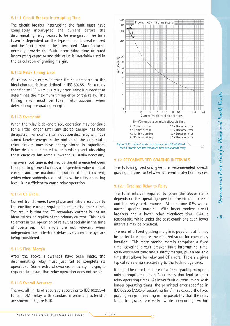
9.11.6 Overall Accuracy
The overall limits of accuracy according to IEC 60255-4for an IDMT relay with standard inverse characteristicare shown in Figure 9.10.
9.12 RECOMMENDED GRADING INTERVALS
The following sections give the recommended overallgrading margins for between different protection devices.
9.12.1 Grading: Relay to Relay
The total interval required to cover the above itemsdepends on the operating speed of the circuit breakersand the relay performance. At one time 0.5s was anormal grading margin. With faster modern circuitbreakers and a lower relay overshoot time, 0.4s isreasonable, while under the best conditions even lowerintervals may be practical.
The use of a fixed grading margin is popular, but it maybe better to calculate the required value for each relaylocation. This more precise margin comprises a fixedtime, covering circuit breaker fault interrupting time,relay overshoot time and a safety margin, plus a variabletime that allows for relay and CT errors. Table 9.2 givestypical relay errors according to the technology used.
It should be noted that use of a fixed grading margin isonly appropriate at high fault levels that lead to shortrelay operating times. At lower fault current levels, withlonger operating times, the permitted error specified inIEC 60255 (7.5% of operating time) may exceed the fixedgrading margin, resulting in the possibility that the relayfails to grade correctly while remaining within
• 9 •O
verc
urre
nt P
rote
ctio
n fo
r Ph
ase
and
Ear
th F
aults
Figure 9.10: Typical limits of accuracy from IEC 60255-4 for an inverse definite minimum time overcurrent relay
Tim
e (s
econ
ds)
2
3
4
6
8
10
1
20
3
40
50
2 3 4 5 6 8 10 20 301
Time/Current characteristic allowable limit
At 2 times settingAt 5 times settingAt 10 times settingAt 20 times setting
2.5 x Declared error1.5 x Declared error1.0 x Declared error1.0 x Declared error

follows an I2t law. So, to achieve proper co-ordinationbetween two fuses in series, it is necessary to ensure thatthe total I2t taken by the smaller fuse is not greater thanthe pre-arcing I2t value of the larger fuse. It has beenestablished by tests that satisfactory grading betweenthe two fuses will generally be achieved if the currentrating ratio between them is greater than two.
9.12.3 Grading: Fuse to Relay
For grading inverse time relays with fuses, the basicapproach is to ensure whenever possible that the relaybacks up the fuse and not vice versa. If the fuse isupstream of the relay, it is very difficult to maintaincorrect discrimination at high values of fault currentbecause of the fast operation of the fuse.
The relay characteristic best suited for this co-ordinationwith fuses is normally the extremely inverse (EI)characteristic as it follows a similar I2t characteristic. Toensure satisfactory co-ordination between relay andfuse, the primary current setting of the relay should beapproximately three times the current rating of the fuse.The grading margin for proper co-ordination, whenexpressed as a fixed quantity, should not be less than0.4s or, when expressed as a variable quantity, shouldhave a minimum value of:
t’ = 0.4t+0.15 seconds …Equation 9.4
where t is the nominal operating time of fuse.
Section 9.20.1 gives an example of fuse to relay grading.
9.13 CALCULATION OF PHASE FAULTOVERCURRENT RELAY SETTINGS
The correct co-ordination of overcurrent relays in a powersystem requires the calculation of the estimated relaysettings in terms of both current and time.
The resultant settings are then traditionally plotted insuitable log/log format to show pictorially that a suitablegrading margin exists between the relays at adjacentsubstations. Plotting may be done by hand, but nowadaysis more commonly achieved using suitable software.
The information required at each relaying point to allowa relay setting calculation to proceed is given in Section9.2. The principal relay data may be tabulated in a tablesimilar to that shown in Table 9.3, if only to assist inrecord keeping.
N e t w o r k P r o t e c t i o n & A u t o m a t i o n G u i d e
specification. This requires consideration whenconsidering the grading margin at low fault current levels.
A practical solution for determining the optimumgrading margin is to assume that the relay nearer to thefault has a maximum possible timing error of +2E, whereE is the basic timing error. To this total effective error forthe relay, a further 10% should be added for the overallcurrent transformer error.
A suitable minimum grading time interval, t’, may becalculated as follows:
…Equation 9.2
where: Er = relay timing error (IEC 60255-4)Ect = allowance for CT ratio error (%)t = operating time of relay nearer fault (s)tCB = CB interrupting time (s)to = relay overshoot time (s)ts = safety margin (s)
If, for example t=0.5s, the time interval for anelectromechanical relay tripping a conventional circuitbreaker would be 0.375s, whereas, at the lower extreme,for a static relay tripping a vacuum circuit breaker, theinterval could be as low as 0.24s.
When the overcurrent relays have independent definitetime delay characteristics, it is not necessary to includethe allowance for CT error. Hence:
…Equation 9.3
Calculation of specific grading times for each relay canoften be tedious when performing a protection gradingcalculation on a power system. Table 9.2 also givespractical grading times at high fault current levelsbetween overcurrent relays for different technologies.Where relays of different technologies are used, the timeappropriate to the technology of the downstream relayshould be used.
9.12.2 Grading: Fuse to Fuse
The operating time of a fuse is a function of both thepre-arcing and arcing time of the fusing element, which
′= ⎡⎣⎢
⎤⎦⎥
+ + +t E t t t tRCB o s
2100
seconds
′= +⎡⎣⎢
⎤⎦⎥
+ + +t E E t t t tR CTCB o s
2100
seconds
• 9 •
Ove
rcur
rent
Pro
tect
ion
for
Phas
e an
d E
arth
Fau
lts
• 1 3 2 •
Fault Current Relay Current Setting(A) Maximun CT Relay Time
Location Load Current Ratio Primary Multiplier SettingMaximun Minimun (A) Per Cent Current
(A)
Table 9.3: Typical relay data table
Table 9.2: Typical relay timing errors - standard IDMT relays
Relay TechnologyElectro- Static Digital Numericalmechanical
Typical basic timing error (%) 7.5 5 5 5
Overshoot time (s) 0.05 0.03 0.02 0.02
Safety margin (s) 0.1 0.05 0.03 0.03
Typical overall grading margin - relay to relay(s) 0.4 0.35 0.3 0.3
N e t w o r k P r o t e c t i o n & A u t o m a t i o n G u i d e • 1 3 3 •
It is usual to plot all time/current characteristics to acommon voltage/MVA base on log/log scales. The plotincludes all relays in a single path, starting with the relaynearest the load and finishing with the relay nearest thesource of supply.
A separate plot is required for each independent path,and the settings of any relays that lie on multiple pathsmust be carefully considered to ensure that the finalsetting is appropriate for all conditions. Earth faults areconsidered separately from phase faults and requireseparate plots.
After relay settings have been finalised, they are enteredin a table. One such table is shown in Table 9.3. This alsoassists in record keeping and during commissioning ofthe relays at site.
9.13.1 Independent (definite) Time Relays
The selection of settings for independent (definite) timerelays presents little difficulty. The overcurrent elementsmust be given settings that are lower, by a reasonablemargin, than the fault current that is likely to flow to afault at the remote end of the system up to which back-up protection is required, with the minimum plant inservice.
The settings must be high enough to avoid relayoperation with the maximum probable load, a suitablemargin being allowed for large motor starting currents ortransformer inrush transients.
Time settings will be chosen to allow suitable gradingmargins, as discussed in Section 9.12.
9.13.2 Inverse Time Relays
When the power system consists of a series of shortsections of cable, so that the total line impedance is low,the value of fault current will be controlled principally bythe impedance of transformers or other fixed plant andwill not vary greatly with the location of the fault. In suchcases, it may be possible to grade the inverse time relaysin very much the same way as definite time relays.However, when the prospective fault current variessubstantially with the location of the fault, it is possible tomake use of this fact by employing both current and timegrading to improve the overall performance of the relay.
The procedure begins by selection of the appropriaterelay characteristics. Current settings are then chosen,with finally the time multiplier settings to giveappropriate grading margins between relays. Otherwise,the procedure is similar to that for definite time delayrelays. An example of a relay setting study is given inSection 9.20.1.
9.14 DIRECTIONAL PHASE FAULT OVERCURRENT RELAYS
When fault current can flow in both directions throughthe relay location, it may be necessary to make theresponse of the relay directional by the introduction of adirectional control facility. The facility is provided by useof additional voltage inputs to the relay.
9.14.1 Relay Connections
There are many possibilities for a suitable connection ofvoltage and current inputs. The various connections aredependent on the phase angle, at unity system powerfactor, by which the current and voltage applied to therelay are displaced. Reference [9.1] details all of theconnections that have been used. However, only very feware used in current practice and these are described below.
In a digital or numerical relay, the phase displacements arerealised by the use of software, while electromechanicaland static relays generally obtain the required phasedisplacements by suitable connection of the inputquantities to the relay. The history of the topic results inthe relay connections being defined as if they wereobtained by suitable connection of the input quantities,irrespective of the actual method used.
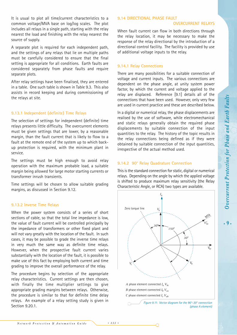
9.14.2 90° Relay Quadrature Connection
This is the standard connection for static, digital or numericalrelays. Depending on the angle by which the applied voltageis shifted to produce maximum relay sensitivity (the RelayCharacteristic Angle, or RCA) two types are available.
• 9 •O
verc
urre
nt P
rote
ctio
n fo
r Ph
ase
and
Ear
th F
aults
Ia
MTA
Zero torque line
VbVc
Vbc
Va
V'bc
30°
30°150°
A phase element connected Ia Vbc
B phase element connected Ib Vca
C phase element connected Ic Vab
Figure 9.11: Vector diagram for the 90°-30° connection (phase A element)

N e t w o r k P r o t e c t i o n & A u t o m a t i o n G u i d e
9.14.2.1 90°-30° characteristic (30° RCA)
The A phase relay element is supplied with Ia current andVbc voltage displaced by 30° in an anti-clockwisedirection. In this case, the relay maximum sensitivity isproduced when the current lags the system phase toneutral voltage by 60°. This connection gives a correctdirectional tripping zone over the current range of 30°leading to 150° lagging; see Figure 9.11. The relaysensitivity at unity power factor is 50% of the relaymaximum sensitivity and 86.6% at zero power factorlagging. This characteristic is recommended when therelay is used for the protection of plain feeders with thezero sequence source behind the relaying point.
9.14.2.2 90°-45° characteristic (45° RCA)
The A phase relay element is supplied with current Ia andvoltage Vbc displaced by 45° in an anti-clockwisedirection. The relay maximum sensitivity is producedwhen the current lags the system phase to neutralvoltage by 45°. This connection gives a correctdirectional tripping zone over the current range of 45°leading to 135° lagging. The relay sensitivity at unitypower factor is 70.7% of the maximum torque and thesame at zero power factor lagging; see Figure 9.12.
This connection is recommended for the protection oftransformer feeders or feeders that have a zero sequencesource in front of the relay. It is essential in the case ofparallel transformers or transformer feeders, in order toensure correct relay operation for faults beyond thestar/delta transformer. This connection should also beused whenever single-phase directional relays areapplied to a circuit where a current distribution of theform 2-1-1 may arise.
For a digital or numerical relay, it is common to allowuser-selection of the RCA angle within a wide range.
Theoretically, three fault conditions can causemaloperation of the directional element:
i. a phase-phase-ground fault on a plain feeder
ii. a phase-ground fault on a transformer feeder withthe zero sequence source in front of the relay
iii. a phase-phase fault on a power transformer withthe relay looking into the delta winding of thetransformer
It should be remembered, however, that the conditionsassumed above to establish the maximum angulardisplacement between the current and voltage quantitiesat the relay are such that, in practice, the magnitude ofthe current input to the relay would be insufficient tocause the overcurrent element to operate. It can beshown analytically that the possibility of maloperationwith the 90°-45° connection is, for all practical purposes,non-existent.
9.14.3 Application of Directional Relays
If non-unit, non-directional relays are applied to parallelfeeders having a single generating source, any faults thatmight occur on any one line will, regardless of the relaysettings used, isolate both lines and completelydisconnect the power supply. With this type of systemconfiguration, it is necessary to apply directional relaysat the receiving end and to grade them with the non-directional relays at the sending end, to ensure correctdiscriminative operation of the relays during line faults.This is done by setting the directional relays R1’ and R2’in Figure 9.13 with their directional elements lookinginto the protected line, and giving them lower time andcurrent settings than relays R1 and R2. The usual practiceis to set relays R1’ and R2’ to 50% of the normal full loadof the protected circuit and 0.1TMS, but care must betaken to ensure that the continuous thermal rating ofthe relays of twice rated current is not exceeded. Anexample calculation is given in Section 9.20.3
• 9 •
Ove
rcur
rent
Prot
ecti
onfo
rPh
ase
and
Ear
thFa
ults
• 1 3 4 •
Fault
Source
R2R'2
R1 R'1
Load
I>
I>I>
I>
Figure 9.13: Directional relays applied to parallel feedersFigure 9.12: Vector diagram for the 90°-45° connection (phase A element)
45°
135°
MTA
Zero torque line
VcVcV VbVbV
VbcVbcV
VaVaV
IaI
V'bc
45°
A phase element connected Ia Vbc
B phase element connected Ib Vca
C phase element connected Ic Vab
N e t w o r k P r o t e c t i o n & A u t o m a t i o n G u i d e • 1 3 5 •
9.15 RING MAINS
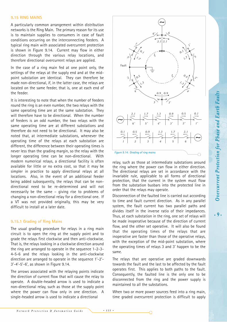
A particularly common arrangement within distributionnetworks is the Ring Main. The primary reason for its useis to maintain supplies to consumers in case of faultconditions occurring on the interconnecting feeders. Atypical ring main with associated overcurrent protectionis shown in Figure 9.14. Current may flow in eitherdirection through the various relay locations, andtherefore directional overcurrent relays are applied.
In the case of a ring main fed at one point only, thesettings of the relays at the supply end and at the mid-point substation are identical. They can therefore bemade non-directional, if, in the latter case, the relays arelocated on the same feeder, that is, one at each end ofthe feeder.
It is interesting to note that when the number of feedersround the ring is an even number, the two relays with thesame operating time are at the same substation. Theywill therefore have to be directional. When the numberof feeders is an odd number, the two relays with thesame operating time are at different substations andtherefore do not need to be directional. It may also benoted that, at intermediate substations, whenever theoperating time of the relays at each substation aredifferent, the difference between their operating times isnever less than the grading margin, so the relay with thelonger operating time can be non-directional. Withmodern numerical relays, a directional facility is oftenavailable for little or no extra cost, so that it may besimpler in practice to apply directional relays at alllocations. Also, in the event of an additional feederbeing added subsequently, the relays that can be non-directional need to be re-determined and will notnecessarily be the same – giving rise to problems ofchanging a non-directional relay for a directional one. Ifa VT was not provided originally, this may be verydifficult to install at a later date.
9.15.1 Grading of Ring Mains
The usual grading procedure for relays in a ring maincircuit is to open the ring at the supply point and tograde the relays first clockwise and then anti-clockwise.That is, the relays looking in a clockwise direction aroundthe ring are arranged to operate in the sequence 1-2-3-4-5-6 and the relays looking in the anti-clockwisedirection are arranged to operate in the sequence 1’-2’-3’-4’-5’-6’, as shown in Figure 9.14.
The arrows associated with the relaying points indicatethe direction of current flow that will cause the relay tooperate. A double-headed arrow is used to indicate anon-directional relay, such as those at the supply pointwhere the power can flow only in one direction. Asingle-headed arrow is used to indicate a directional
relay, such as those at intermediate substations aroundthe ring where the power can flow in either direction.The directional relays are set in accordance with theinvariable rule, applicable to all forms of directionalprotection, that the current in the system must flowfrom the substation busbars into the protected line inorder that the relays may operate.Disconnection of the faulted line is carried out accordingto time and fault current direction. As in any parallelsystem, the fault current has two parallel paths anddivides itself in the inverse ratio of their impedances.Thus, at each substation in the ring, one set of relays willbe made inoperative because of the direction of currentflow, and the other set operative. It will also be foundthat the operating times of the relays that areinoperative are faster than those of the operative relays,with the exception of the mid-point substation, wherethe operating times of relays 3 and 3’ happen to be thesame.
The relays that are operative are graded downwardstowards the fault and the last to be affected by the faultoperates first. This applies to both paths to the fault.Consequently, the faulted line is the only one to bedisconnected from the ring and the power supply ismaintained to all the substations.
When two or more power sources feed into a ring main,time graded overcurrent protection is difficult to apply
• 9 •O
verc
urre
nt P
rote
ctio
n fo
r Ph
ase
and
Ear
th F
aults
Figure 9.14: Grading of ring mains
2.1 2.1
6' 6
0.9
3'
1.7
0.1
5'
1
0.52
4'
1.3
1.7 50.1
1'
0.9
3
1.3
0.5
4
2'
Fault
2.1
6'
1.7
5' '4' '3
1.3 0.9
2'
0.5
'1
0.1
654
2.11.71.3
321
0.90.50.1
Ix
Iy
N e t w o r k P r o t e c t i o n & A u t o m a t i o n G u i d e
and full discrimination may not be possible. With twosources of supply, two solutions are possible. The first isto open the ring at one of the supply points, whichever ismore convenient, by means of a suitable high setinstantaneous overcurrent relay. The ring is then gradedas in the case of a single infeed. The second method is totreat the section of the ring between the two supplypoints as a continuous bus separate from the ring and toprotect it with a unit protection system, and then proceedto grade the ring as in the case of a single infeed. Section9.20.4 provides a worked example of ring main grading.
9.16 EARTH FAULT PROTECTION
In the foregoing description, attention has beenprincipally directed towards phase fault overcurrentprotection. More sensitive protection against earthfaults can be obtained by using a relay that respondsonly to the residual current of the system, since aresidual component exists only when fault current flowsto earth. The earth-fault relay is therefore completelyunaffected by load currents, whether balanced or not,and can be given a setting which is limited only by thedesign of the equipment and the presence of unbalancedleakage or capacitance currents to earth. This is animportant consideration if settings of only a few percentof system rating are considered, since leakage currentsmay produce a residual quantity of this order.
On the whole, the low settings permissible for earth-fault relays are very useful, as earth faults are not onlyby far the most frequent of all faults, but may be limitedin magnitude by the neutral earthing impedance, or byearth contact resistance.
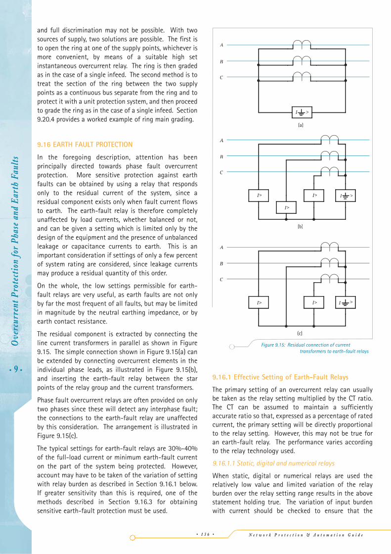
The residual component is extracted by connecting theline current transformers in parallel as shown in Figure9.15. The simple connection shown in Figure 9.15(a) canbe extended by connecting overcurrent elements in theindividual phase leads, as illustrated in Figure 9.15(b),and inserting the earth-fault relay between the starpoints of the relay group and the current transformers.
Phase fault overcurrent relays are often provided on onlytwo phases since these will detect any interphase fault;the connections to the earth-fault relay are unaffectedby this consideration. The arrangement is illustrated inFigure 9.15(c).
The typical settings for earth-fault relays are 30%-40%of the full-load current or minimum earth-fault currenton the part of the system being protected. However,account may have to be taken of the variation of settingwith relay burden as described in Section 9.16.1 below.If greater sensitivity than this is required, one of themethods described in Section 9.16.3 for obtainingsensitive earth-fault protection must be used.
9.16.1 Effective Setting of Earth-Fault Relays
The primary setting of an overcurrent relay can usuallybe taken as the relay setting multiplied by the CT ratio.The CT can be assumed to maintain a sufficientlyaccurate ratio so that, expressed as a percentage of ratedcurrent, the primary setting will be directly proportionalto the relay setting. However, this may not be true foran earth-fault relay. The performance varies accordingto the relay technology used.
9.16.1.1 Static, digital and numerical relays
When static, digital or numerical relays are used therelatively low value and limited variation of the relayburden over the relay setting range results in the abovestatement holding true. The variation of input burdenwith current should be checked to ensure that the
• 9 •
Ove
rcur
rent
Pro
tect
ion
for
Phas
e an
d E
arth
Fau
lts
• 1 3 6 •
A
B
C
C
B
A
C
B
A
(c)
(b)
(a)
I >
I>
I>
I> I >
I>I> I >
Figure 9.15: Residual connection of current transformers to earth-fault relays
N e t w o r k P r o t e c t i o n & A u t o m a t i o n G u i d e • 1 3 7 •
variation is sufficiently small. If not, substantial errorsmay occur, and the setting procedure will have to followthat for electromechanical relays.
9.16.1.2 Electromechanical relays
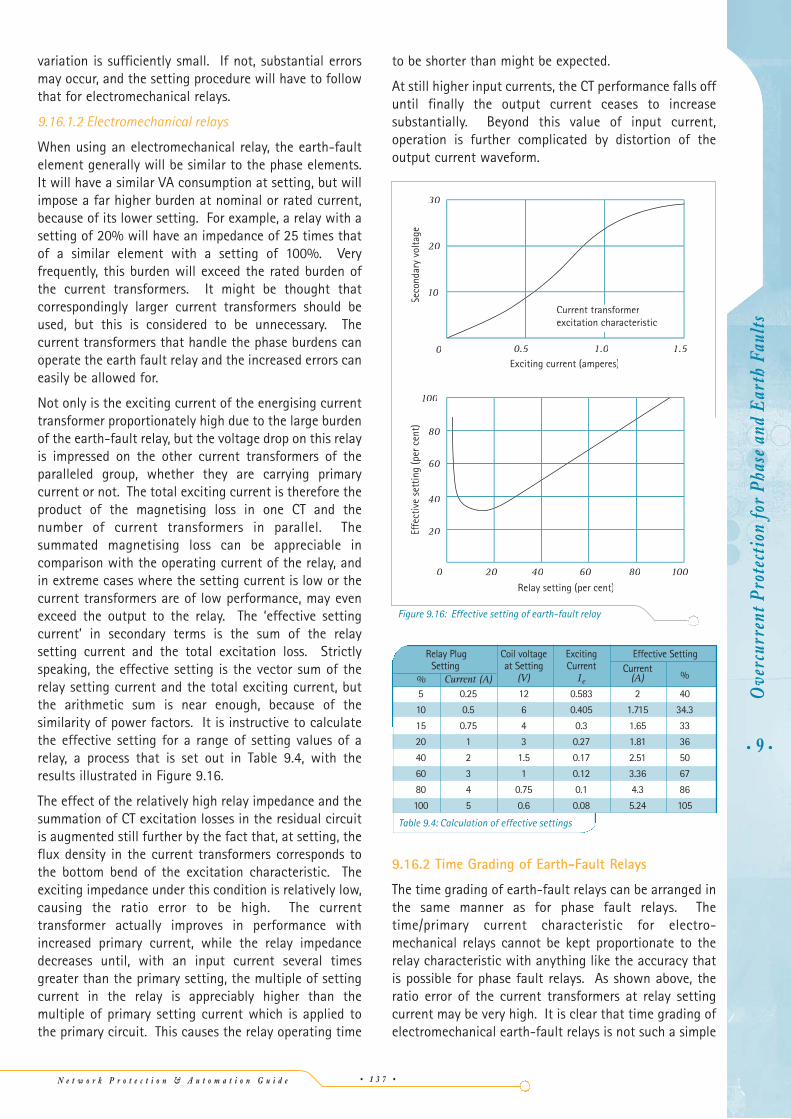
When using an electromechanical relay, the earth-faultelement generally will be similar to the phase elements.It will have a similar VA consumption at setting, but willimpose a far higher burden at nominal or rated current,because of its lower setting. For example, a relay with asetting of 20% will have an impedance of 25 times thatof a similar element with a setting of 100%. Veryfrequently, this burden will exceed the rated burden ofthe current transformers. It might be thought thatcorrespondingly larger current transformers should beused, but this is considered to be unnecessary. Thecurrent transformers that handle the phase burdens canoperate the earth fault relay and the increased errors caneasily be allowed for.
Not only is the exciting current of the energising currenttransformer proportionately high due to the large burdenof the earth-fault relay, but the voltage drop on this relayis impressed on the other current transformers of theparalleled group, whether they are carrying primarycurrent or not. The total exciting current is therefore theproduct of the magnetising loss in one CT and thenumber of current transformers in parallel. Thesummated magnetising loss can be appreciable incomparison with the operating current of the relay, andin extreme cases where the setting current is low or thecurrent transformers are of low performance, may evenexceed the output to the relay. The ‘effective settingcurrent’ in secondary terms is the sum of the relaysetting current and the total excitation loss. Strictlyspeaking, the effective setting is the vector sum of therelay setting current and the total exciting current, butthe arithmetic sum is near enough, because of thesimilarity of power factors. It is instructive to calculatethe effective setting for a range of setting values of arelay, a process that is set out in Table 9.4, with theresults illustrated in Figure 9.16.
The effect of the relatively high relay impedance and thesummation of CT excitation losses in the residual circuitis augmented still further by the fact that, at setting, theflux density in the current transformers corresponds tothe bottom bend of the excitation characteristic. Theexciting impedance under this condition is relatively low,causing the ratio error to be high. The currenttransformer actually improves in performance withincreased primary current, while the relay impedancedecreases until, with an input current several timesgreater than the primary setting, the multiple of settingcurrent in the relay is appreciably higher than themultiple of primary setting current which is applied tothe primary circuit. This causes the relay operating time
to be shorter than might be expected.
At still higher input currents, the CT performance falls offuntil finally the output current ceases to increasesubstantially. Beyond this value of input current,operation is further complicated by distortion of theoutput current waveform.
9.16.2 Time Grading of Earth-Fault Relays
The time grading of earth-fault relays can be arranged inthe same manner as for phase fault relays. Thetime/primary current characteristic for electro-mechanical relays cannot be kept proportionate to therelay characteristic with anything like the accuracy thatis possible for phase fault relays. As shown above, theratio error of the current transformers at relay settingcurrent may be very high. It is clear that time grading ofelectromechanical earth-fault relays is not such a simple
• 9 •O
verc
urre
nt P
rote
ctio
n fo
r Ph
ase
and
Ear
th F
aults
Table 9.4: Calculation of effective settings
Relay Plug Coil voltage Exciting Effective SettingSetting at Setting Current Current
%% Current (A) (V) Ie (A)
5 0.25 12 0.583 2 40
10 0.5 6 0.405 1.715 34.3
15 0.75 4 0.3 1.65 33
20 1 3 0.27 1.81 36
40 2 1.5 0.17 2.51 50
60 3 1 0.12 3.36 67
80 4 0.75 0.1 4.3 86
100 5 0.6 0.08 5.24 105
Figure 9.16: Effective setting of earth-fault relay
Current transformerexcitation characteristic
1.51.00.50
10
20
30
Seco
ndar
y vo
ltage
Exciting current (amperes)
Effe
ctiv
e se
ttin
g (p
er c
ent)
0 80 100
100
80
60
40
20
604020
Relay setting (per cent)
N e t w o r k P r o t e c t i o n & A u t o m a t i o n G u i d e
matter as the procedure adopted for phase relays in Table 9.3. Either the above factors must be taken intoaccount with the errors calculated for each current level,making the process much more tedious, or longergrading margins must be allowed. However, for othertypes of relay, the procedure adopted for phase faultrelays can be used.
9.16.3 Sensitive Earth-Fault Protection
LV systems are not normally earthed through animpedance, due to the resulting overvoltages that mayoccur and consequential safety implications. HV systemsmay be designed to accommodate such overvoltages, butnot the majority of LV systems.
However, it is quite common to earth HV systems throughan impedance that limits the earth-fault current. Further,in some countries, the resistivity of the earth path may bevery high due to the nature of the ground itself (e.g.desert or rock). A fault to earth not involving earthconductors may result in the flow of only a small current,insufficient to operate a normal protection system. Asimilar difficulty also arises in the case of broken lineconductors, which, after falling on to hedges or drymetalled roads, remain energised because of the lowleakage current, and therefore present a danger to life.
To overcome the problem, it is necessary to provide anearth-fault protection system with a setting that isconsiderably lower than the normal line protection. Thispresents no difficulty to a modern digital or numericalrelay. However, older electromechanical or static relaysmay present difficulties due to the high effective burdenthey may present to the CT.
The required sensitivity cannot normally be provided bymeans of conventional CT’s. A core balance currenttransformer (CBCT) will normally be used. The CBCT is acurrent transformer mounted around all three phase (andneutral if present) conductors so that the CT secondarycurrent is proportional to the residual (i.e. earth) current.Such a CT can be made to have any convenient ratiosuitable for operating a sensitive earth-fault relayelement. By use of such techniques, earth fault settingsdown to 10% of the current rating of the circuit to beprotected can be obtained.
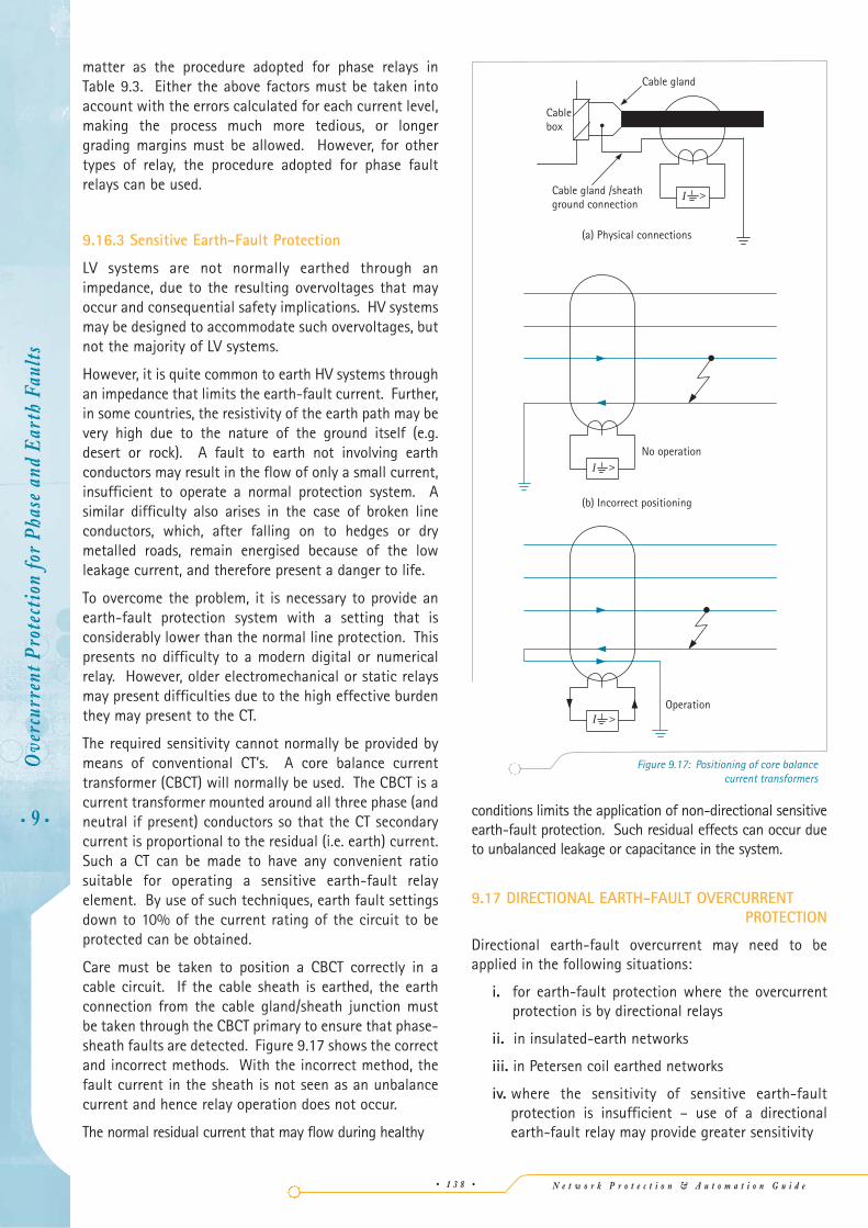
Care must be taken to position a CBCT correctly in acable circuit. If the cable sheath is earthed, the earthconnection from the cable gland/sheath junction mustbe taken through the CBCT primary to ensure that phase-sheath faults are detected. Figure 9.17 shows the correctand incorrect methods. With the incorrect method, thefault current in the sheath is not seen as an unbalancecurrent and hence relay operation does not occur.
The normal residual current that may flow during healthy
conditions limits the application of non-directional sensitiveearth-fault protection. Such residual effects can occur dueto unbalanced leakage or capacitance in the system.
9.17 DIRECTIONAL EARTH-FAULT OVERCURRENTPROTECTION
Directional earth-fault overcurrent may need to beapplied in the following situations:
i. for earth-fault protection where the overcurrentprotection is by directional relays
ii. in insulated-earth networks
iii. in Petersen coil earthed networks
iv. where the sensitivity of sensitive earth-faultprotection is insufficient – use of a directionalearth-fault relay may provide greater sensitivity
• 9 •
Ove
rcur
rent
Pro
tect
ion
for
Phas
e an
d E
arth
Fau
lts
• 1 3 8 •
Cable gland /sheathground connection
(a) Physical connections
(b) Incorrect positioning
Cable gland
Cablebox
No operation
Operation
I >
I >
I >
Figure 9.17: Positioning of core balance current transformers
N e t w o r k P r o t e c t i o n & A u t o m a t i o n G u i d e • 1 3 9 •
The relay elements previously described as phase faultelements respond to the flow of earth fault current, andit is important that their directional response be correctfor this condition. If a special earth fault element isprovided as described in Section 9.16 (which will normallybe the case), a related directional element is needed.
9.17.1 Relay Connections
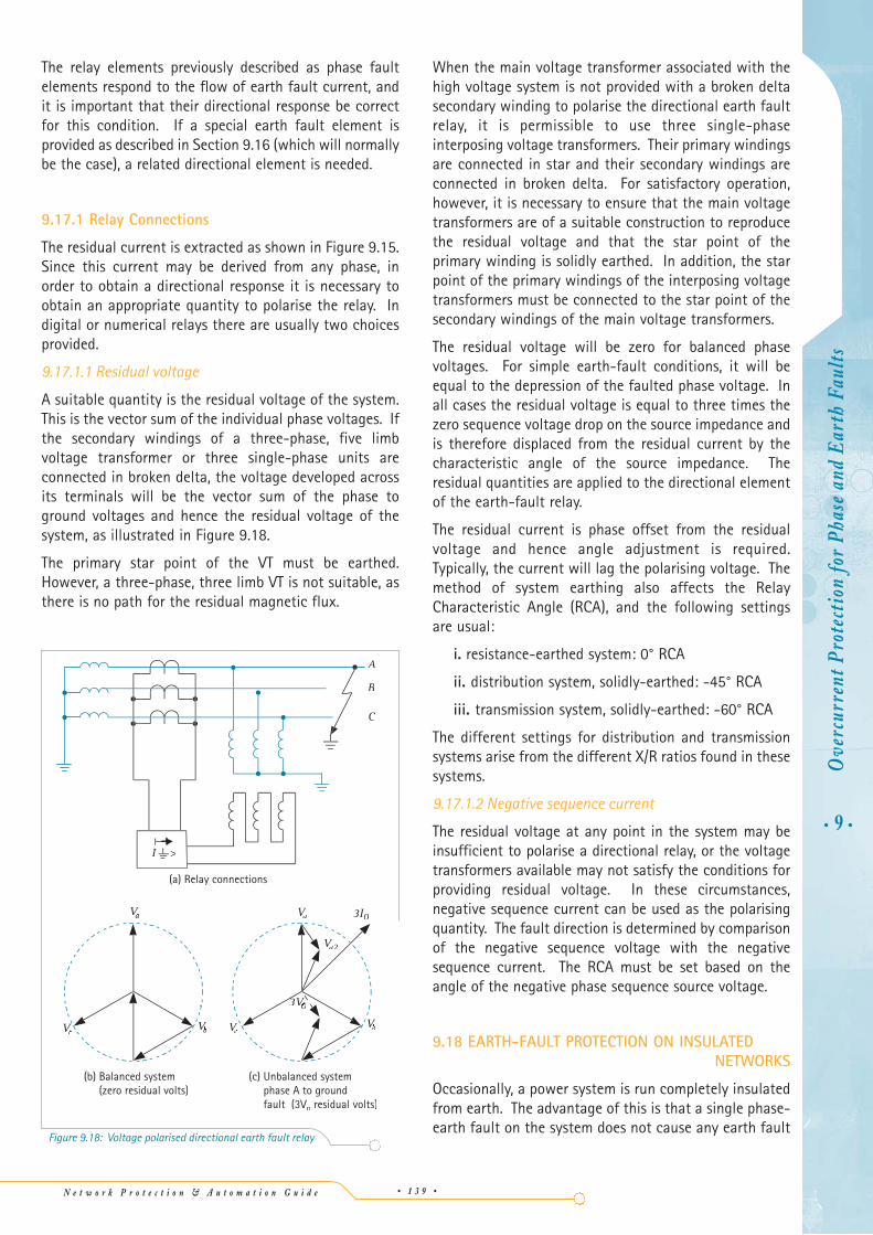
The residual current is extracted as shown in Figure 9.15.Since this current may be derived from any phase, inorder to obtain a directional response it is necessary toobtain an appropriate quantity to polarise the relay. Indigital or numerical relays there are usually two choicesprovided.
9.17.1.1 Residual voltage
A suitable quantity is the residual voltage of the system.This is the vector sum of the individual phase voltages. Ifthe secondary windings of a three-phase, five limbvoltage transformer or three single-phase units areconnected in broken delta, the voltage developed acrossits terminals will be the vector sum of the phase toground voltages and hence the residual voltage of thesystem, as illustrated in Figure 9.18.
The primary star point of the VT must be earthed.However, a three-phase, three limb VT is not suitable, asthere is no path for the residual magnetic flux.
When the main voltage transformer associated with thehigh voltage system is not provided with a broken deltasecondary winding to polarise the directional earth faultrelay, it is permissible to use three single-phaseinterposing voltage transformers. Their primary windingsare connected in star and their secondary windings areconnected in broken delta. For satisfactory operation,however, it is necessary to ensure that the main voltagetransformers are of a suitable construction to reproducethe residual voltage and that the star point of theprimary winding is solidly earthed. In addition, the starpoint of the primary windings of the interposing voltagetransformers must be connected to the star point of thesecondary windings of the main voltage transformers.
The residual voltage will be zero for balanced phasevoltages. For simple earth-fault conditions, it will beequal to the depression of the faulted phase voltage. Inall cases the residual voltage is equal to three times thezero sequence voltage drop on the source impedance andis therefore displaced from the residual current by thecharacteristic angle of the source impedance. Theresidual quantities are applied to the directional elementof the earth-fault relay.
The residual current is phase offset from the residualvoltage and hence angle adjustment is required.Typically, the current will lag the polarising voltage. Themethod of system earthing also affects the RelayCharacteristic Angle (RCA), and the following settingsare usual:
i. resistance-earthed system: 0° RCA
ii. distribution system, solidly-earthed: -45° RCA
iii. transmission system, solidly-earthed: -60° RCA
The different settings for distribution and transmissionsystems arise from the different X/R ratios found in thesesystems.
9.17.1.2 Negative sequence current
The residual voltage at any point in the system may beinsufficient to polarise a directional relay, or the voltagetransformers available may not satisfy the conditions forproviding residual voltage. In these circumstances,negative sequence current can be used as the polarisingquantity. The fault direction is determined by comparisonof the negative sequence voltage with the negativesequence current. The RCA must be set based on theangle of the negative phase sequence source voltage.
9.18 EARTH-FAULT PROTECTION ON INSULATEDNETWORKS
Occasionally, a power system is run completely insulatedfrom earth. The advantage of this is that a single phase-earth fault on the system does not cause any earth fault
• 9 •O
verc
urre
nt P
rote
ctio
n fo
r Ph
ase
and
Ear
th F
aults
Figure 9.18: Voltage polarised directional earth fault relay
(a) Relay connections
C
B
A
VaVV
VcVV VbVV VcVV VbVV
Va2VV
3IOII
3VOVV
VaVV
(b) Balanced system (zero residual volts)
(c) Unbalanced system
fault (3Vo residual volts)
3
>I
N e t w o r k P r o t e c t i o n & A u t o m a t i o n G u i d e
current to flow, and so the whole system remainsoperational. The system must be designed to withstand hightransient and steady-state overvoltages however, so its useis generally restricted to low and medium voltage systems.
It is vital that detection of a single phase-earth fault isachieved, so that the fault can be traced and rectified.While system operation is unaffected for this condition,the occurrence of a second earth fault allows substantialcurrents to flow.
The absence of earth-fault current for a single phase-earthfault clearly presents some difficulties in fault detection.Two methods are available using modern relays.
9.18.1 Residual Voltage
When a single phase-earth fault occurs, the healthyphase voltages rise by a factor of √3 and the three phasevoltages no longer have a phasor sum of zero. Hence, aresidual voltage element can be used to detect the fault.However, the method does not provide anydiscrimination, as the unbalanced voltage occurs on thewhole of the affected section of the system. Oneadvantage of this method is that no CT’s are required, asvoltage is being measured. However, the requirementsfor the VT’s as given in Section 9.17.1.1 apply.
Grading is a problem with this method, since all relays inthe affected section will see the fault. It may be possibleto use definite-time grading, but in general, it is notpossible to provide fully discriminative protection usingthis technique.
9.18.2 Sensitive Earth Fault
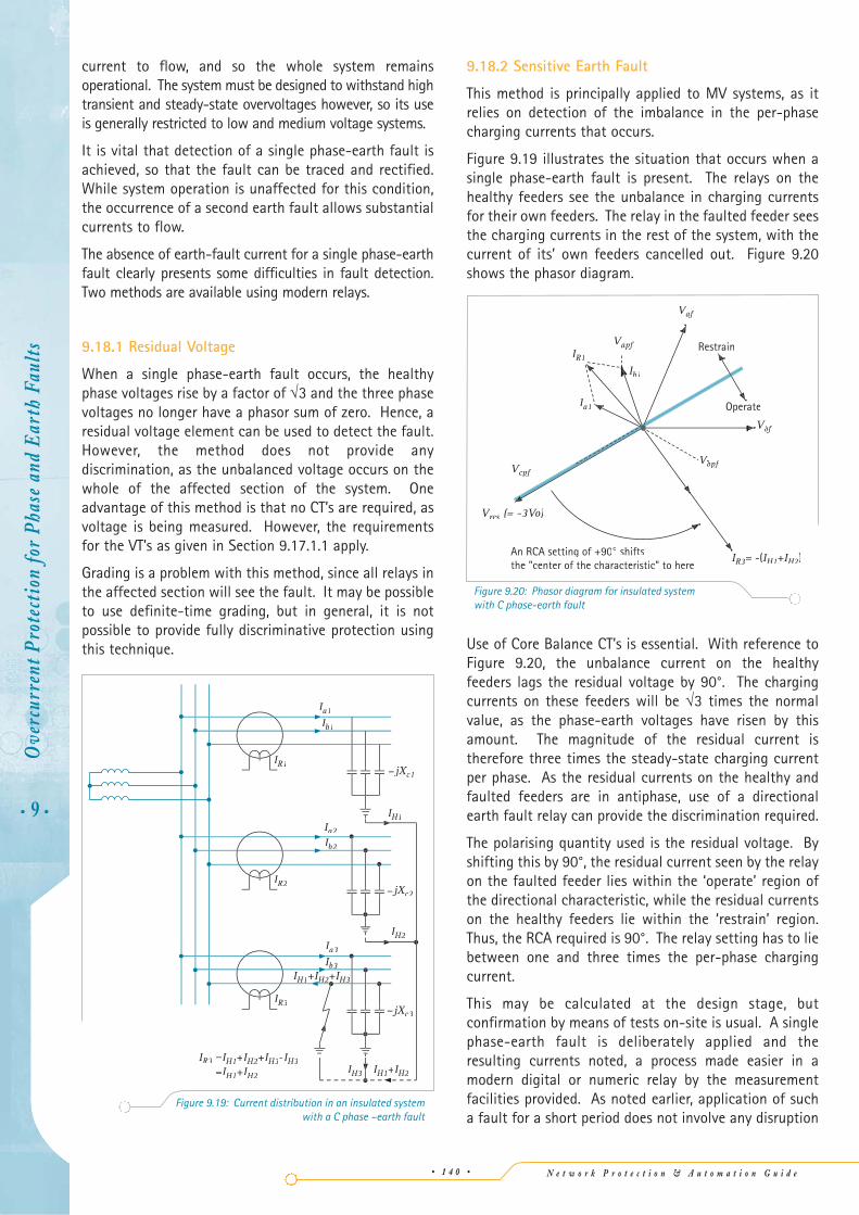
This method is principally applied to MV systems, as itrelies on detection of the imbalance in the per-phasecharging currents that occurs.
Figure 9.19 illustrates the situation that occurs when asingle phase-earth fault is present. The relays on thehealthy feeders see the unbalance in charging currentsfor their own feeders. The relay in the faulted feeder seesthe charging currents in the rest of the system, with thecurrent of its’ own feeders cancelled out. Figure 9.20shows the phasor diagram.
Use of Core Balance CT’s is essential. With reference toFigure 9.20, the unbalance current on the healthyfeeders lags the residual voltage by 90°. The chargingcurrents on these feeders will be √3 times the normalvalue, as the phase-earth voltages have risen by thisamount. The magnitude of the residual current istherefore three times the steady-state charging currentper phase. As the residual currents on the healthy andfaulted feeders are in antiphase, use of a directionalearth fault relay can provide the discrimination required.
The polarising quantity used is the residual voltage. Byshifting this by 90°, the residual current seen by the relayon the faulted feeder lies within the ‘operate’ region ofthe directional characteristic, while the residual currentson the healthy feeders lie within the ‘restrain’ region.Thus, the RCA required is 90°. The relay setting has to liebetween one and three times the per-phase chargingcurrent.
This may be calculated at the design stage, butconfirmation by means of tests on-site is usual. A singlephase-earth fault is deliberately applied and theresulting currents noted, a process made easier in amodern digital or numeric relay by the measurementfacilities provided. As noted earlier, application of sucha fault for a short period does not involve any disruption
• 9 •
Ove
rcur
rent
Pro
tect
ion
for
Phas
e an
d E
arth
Fau
lts
• 1 4 0 •
Ia3II
IH1I + H3
I +IH2II
IR3I
IR2I
IR1I
IH2I
I
Ia2IIIb2II
Ia1IIIb1II
jXc3XX
jXc2XX
IH1I
jXc1XX
=I +IH2I +IH3I -IH3I=IH1I IH2I
IR3I
Figure 9.19: Current distribution in an insulated system with a C phase –earth fault
Figure 9.20: Phasor diagram for insulated system with C phase-earth fault
An RCA setting of +90° shiftsthe "center of the characteristic" to here
VcpfVVVbpfVV
VbfVV
IR3I = -(IH1I IH2II )
VafVV
VapfVVIR1I
Ia1II
Ib1II
Restrain
Operate
VresVV (= -3Vo)
N e t w o r k P r o t e c t i o n & A u t o m a t i o n G u i d e • 1 4 1 •
to the network, or fault currents, but the duration shouldbe as short as possible to guard against a second suchfault occurring.
It is also possible to dispense with the directional elementif the relay can be set at a current value that lies betweenthe charging current on the feeder to be protected andthe charging current of the rest of the system.
9.19 EARTH FAULT PROTECTION ON PETERSEN COILEARTHED NETWORKS
Petersen Coil earthing is a special case of highimpedance earthing. The network is earthed via areactor, whose reactance is made nominally equal to thetotal system capacitance to earth. Under this condition,a single phase-earth fault does not result in any earthfault current in steady-state conditions. The effect istherefore similar to having an insulated system. Theeffectiveness of the method is dependent on theaccuracy of tuning of the reactance value – changes insystem capacitance (due to system configurationchanges for instance) require changes to the coilreactance. In practice, perfect matching of the coilreactance to the system capacitance is difficult toachieve, so that a small earth fault current will flow.Petersen Coil earthed systems are commonly found inareas where the system consists mainly of rural overheadlines, and are particularly beneficial in locations subjectto a high incidence of transient faults.
To understand how to correctly apply earth faultprotection to such systems, system behaviour under earthfault conditions must first be understood.
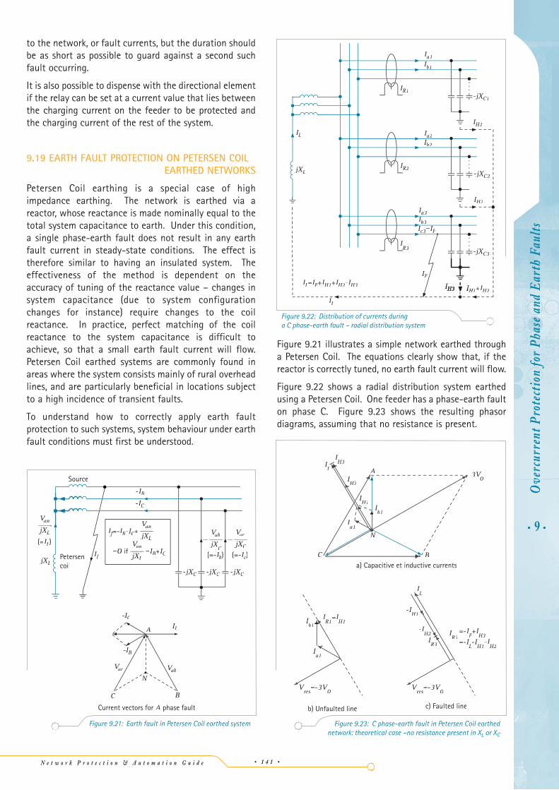
Figure 9.21 illustrates a simple network earthed througha Petersen Coil. The equations clearly show that, if thereactor is correctly tuned, no earth fault current will flow.
Figure 9.22 shows a radial distribution system earthedusing a Petersen Coil. One feeder has a phase-earth faulton phase C. Figure 9.23 shows the resulting phasordiagrams, assuming that no resistance is present.
• 9 •O
verc
urre
nt P
rote
ctio
n fo
r Ph
ase
and
Ear
th F
aults
C B
A ILI
-IBI
-ICII
VabVVVacVV
-----
N
Current vectors for A phase fault
Source
Petersencoil
-ICII
-jX- CXX-jX- X
jXLXX
(=ILII )
VanVV
L
-jX- CXX
(=-IbII
VabVV
jXC
XIcII )
VacVV
CIfII
-IBI
IfIIf IBI - C+VanVV
jXLXX
=O if =IBI +ICIIan
jXLX
Figure 9.21: Earth fault in Petersen Coil earthed system
A
N
C B
3VO
VVIL
IH3
IH2
IH1
b1
Ia1
Ib1II
IL
IR3
Ia1
IR1
=IH1
Vres
=-3VO
V Vres
=-3VO
V
a) Capacitive et inductive currents
b) Unfaulted line c) Faulted line
-IH1
IR3
=-I +I=- -I
H2
-I
Figure 9.23: C phase-earth fault in Petersen Coil earthed network: theoretical case –no resistance present in XL or XC
ILI =IFII IH1I IH2I -IH3IH1+IH2I
ILI
IFII
IH2IIa3II
II =IFIIb3II
Ia2IIb2II
IR3
IR2I
-jX- C3XX
-jX- C2XXjXLXX
ILIIH1I
Ia1IIb1II
IR1I-jX- C1XX
Figure 9.22: Distribution of currents during a C phase-earth fault – radial distribution system
N e t w o r k P r o t e c t i o n & A u t o m a t i o n G u i d e
In Figure 9.23(a), it can be seen that the fault causes thehealthy phase voltages to rise by a factor of √3 and thecharging currents lead the voltages by 90°.
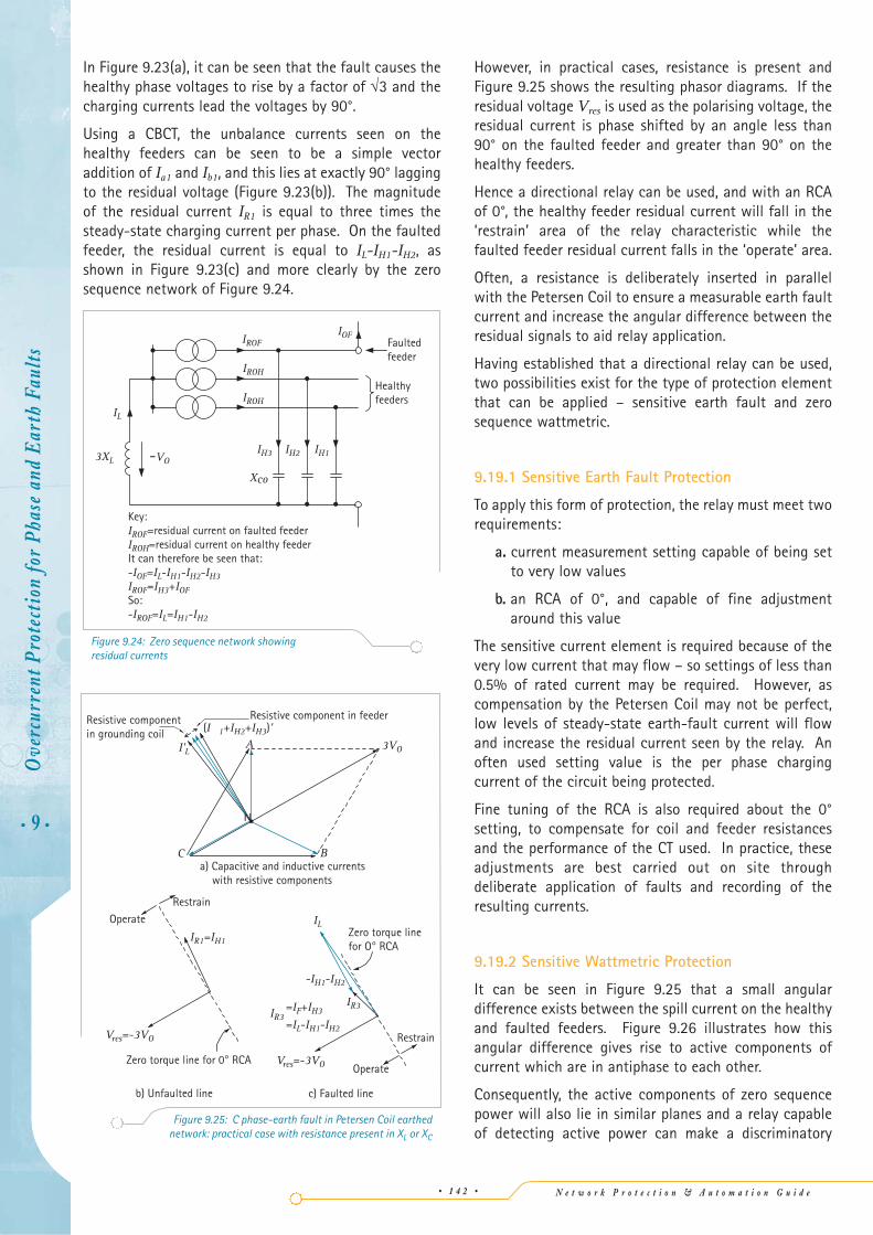
Using a CBCT, the unbalance currents seen on thehealthy feeders can be seen to be a simple vectoraddition of Ia1 and Ib1, and this lies at exactly 90° laggingto the residual voltage (Figure 9.23(b)). The magnitudeof the residual current IR1 is equal to three times thesteady-state charging current per phase. On the faultedfeeder, the residual current is equal to IL-IH1-IH2, asshown in Figure 9.23(c) and more clearly by the zerosequence network of Figure 9.24.
However, in practical cases, resistance is present andFigure 9.25 shows the resulting phasor diagrams. If theresidual voltage Vres is used as the polarising voltage, theresidual current is phase shifted by an angle less than90° on the faulted feeder and greater than 90° on thehealthy feeders.
Hence a directional relay can be used, and with an RCAof 0°, the healthy feeder residual current will fall in the‘restrain’ area of the relay characteristic while thefaulted feeder residual current falls in the ‘operate’ area.
Often, a resistance is deliberately inserted in parallelwith the Petersen Coil to ensure a measurable earth faultcurrent and increase the angular difference between theresidual signals to aid relay application.
Having established that a directional relay can be used,two possibilities exist for the type of protection elementthat can be applied – sensitive earth fault and zerosequence wattmetric.
9.19.1 Sensitive Earth Fault Protection
To apply this form of protection, the relay must meet tworequirements:
a. current measurement setting capable of being setto very low values
b. an RCA of 0°, and capable of fine adjustmentaround this value
The sensitive current element is required because of thevery low current that may flow – so settings of less than0.5% of rated current may be required. However, ascompensation by the Petersen Coil may not be perfect,low levels of steady-state earth-fault current will flowand increase the residual current seen by the relay. Anoften used setting value is the per phase chargingcurrent of the circuit being protected.
Fine tuning of the RCA is also required about the 0°setting, to compensate for coil and feeder resistancesand the performance of the CT used. In practice, theseadjustments are best carried out on site throughdeliberate application of faults and recording of theresulting currents.
9.19.2 Sensitive Wattmetric Protection
It can be seen in Figure 9.25 that a small angulardifference exists between the spill current on the healthyand faulted feeders. Figure 9.26 illustrates how thisangular difference gives rise to active components ofcurrent which are in antiphase to each other.
Consequently, the active components of zero sequencepower will also lie in similar planes and a relay capableof detecting active power can make a discriminatory
• 9 •
Ove
rcur
rent
Pro
tect
ion
for
Phas
e an
d E
arth
Fau
lts
• 1 4 2 •
IL
IH3
IROFIOF
IROH
IROH
Xco
IH2 IH13XL
Faulted feeder
Healthy feeders
Key:IROF=residual current on faulted feederIROH=residual current on healthy feederIt can therefore be seen that:-IOF=IL-IH1-IH2-IH3IROF=IH3+IOFSo:-IROF=IL=IH1-IH2
-VO
Figure 9.24: Zero sequence network showing residual currents
A
N
C B
I'L
(I 1+IH2+IH3)'
IR1=IH1
Vres=-3VO
Vres=-3VO
-IH1-IH2
3VO
IL
IR3=IF+IH3
=IL-IH1-IH2
IR3
b) Unfaulted line
Resistive component in feederResistive componentin grounding coil
Restrain
Zero torque line for 0° RCA
c) Faulted line
Operate
Operate
Restrain
Zero torque linefor O° RCA
a) Capacitive and inductive currents with resistive components
Figure 9.25: C phase-earth fault in Petersen Coil earthed network: practical case with resistance present in XL or XC
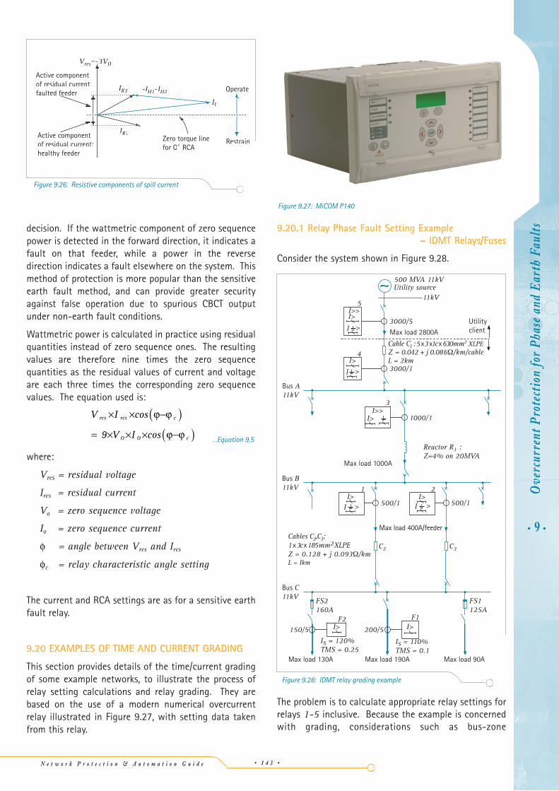
N e t w o r k P r o t e c t i o n & A u t o m a t i o n G u i d e • 1 4 3 •
decision. If the wattmetric component of zero sequencepower is detected in the forward direction, it indicates afault on that feeder, while a power in the reversedirection indicates a fault elsewhere on the system. Thismethod of protection is more popular than the sensitiveearth fault method, and can provide greater securityagainst false operation due to spurious CBCT outputunder non-earth fault conditions.
Wattmetric power is calculated in practice using residualquantities instead of zero sequence ones. The resultingvalues are therefore nine times the zero sequencequantities as the residual values of current and voltageare each three times the corresponding zero sequencevalues. The equation used is:
…Equation 9.5
where:
Vres = residual voltage
Ires = residual current
Vo = zero sequence voltage
Io = zero sequence current
φ = angle between Vres and Ires
φc = relay characteristic angle setting
The current and RCA settings are as for a sensitive earthfault relay.
9.20 EXAMPLES OF TIME AND CURRENT GRADING
This section provides details of the time/current gradingof some example networks, to illustrate the process ofrelay setting calculations and relay grading. They arebased on the use of a modern numerical overcurrentrelay illustrated in Figure 9.27, with setting data takenfrom this relay.
V I
V I
res res c
O O c
× × −( )= × × × −( )
cos
cos
ϕ ϕ
ϕ ϕ 9
9.20.1 Relay Phase Fault Setting Example – IDMT Relays/Fuses
Consider the system shown in Figure 9.28.
The problem is to calculate appropriate relay settings forrelays 1-5 inclusive. Because the example is concernedwith grading, considerations such as bus-zone
• 9 •O
verc
urre
nt P
rote
ctio
n fo
r Ph
ase
and
Ear
th F
aults
Active componentof residual current:faulted feeder
Zero torque linefor O° RCA
Operate
RestrainIR1I
ILII
IR3I IH1II -IH2I
VresVV =-3VOVV
of residual current:healthy feeder
Figure 9.26: Resistive components of spill current
I>>
I>>
I>
I>
I>
I>
I
I
I
500 MVA 11kVUtility source
11kV
Max load 2800A
Utility client
Cable C1 : 5 x 3 x1c x 630mm2 XLPEZ = 0.042 + j 0.086Ω/km/cableL = 2km
3000/5
Bus A 11kV
Bus B 11kV
Bus C 11kV
150/5 200/5
C3C2
4
5
3000/1
Cables C2,C3: 1 x 3c x 185mm2XLPEZ = 0.128 + j 0.093Ω/kmL = Ikm
>
>
>I>
I>I>
I >
Max load 400A/feeder
1
500/1500/1
1000/1
3
Max load 1000A
Reactor R1 : Z=4% on 20MVA
2
Max load 190AMax load 130A Max load 90A
IS = 120%TMS = 0.25
IS = 110%TMS = 0.1
FS2160A
FS1125A
F2 F1
Figure 9.28: IDMT relay grading example
Figure 9.27: MiCOM P140
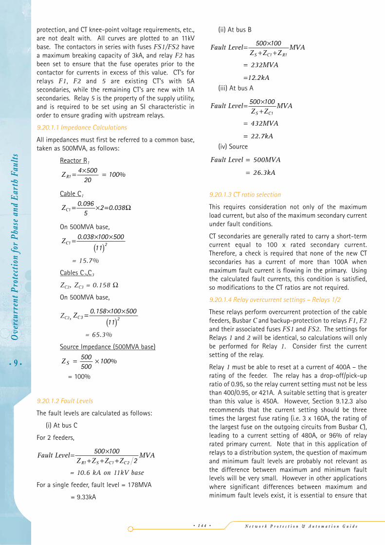
N e t w o r k P r o t e c t i o n & A u t o m a t i o n G u i d e
protection, and CT knee-point voltage requirements, etc.,are not dealt with. All curves are plotted to an 11kVbase. The contactors in series with fuses FS1/FS2 havea maximum breaking capacity of 3kA, and relay F2 hasbeen set to ensure that the fuse operates prior to thecontactor for currents in excess of this value. CT’s forrelays F1, F2 and 5 are existing CT’s with 5Asecondaries, while the remaining CT’s are new with 1Asecondaries. Relay 5 is the property of the supply utility,and is required to be set using an SI characteristic inorder to ensure grading with upstream relays.
9.20.1.1 Impedance Calculations
All impedances must first be referred to a common base,taken as 500MVA, as follows:
Reactor R1
Cable C1
On 500MVA base,
= 15.7%
Cables C2,C3
ZC2, ZC3 = 0.158 Ω
On 500MVA base,
ZC2,
= 65.3%
Source Impedance (500MVA base)
= 100%
9.20.1.2 Fault Levels
The fault levels are calculated as follows:
(i) At bus C
For 2 feeders,
= 10.6 kA on 11kV base
For a single feeder, fault level = 178MVA
= 9.33kA
Fault Level= ×+ + +
500 10021 1 2Z Z Z Z
MVAR S C C
ZS = ×500500
100%
ZC3 2
0 158 100 500
11= × ×
( ).
ZC1 2
0 038 100 500
11= × ×
( ).
ZC10 096
52 0 038= × =. . Ω
ZR14 500
20100= × = %
(ii) At bus B
(iii) At bus A
(iv) Source
9.20.1.3 CT ratio selection
This requires consideration not only of the maximumload current, but also of the maximum secondary currentunder fault conditions.
CT secondaries are generally rated to carry a short-termcurrent equal to 100 x rated secondary current.Therefore, a check is required that none of the new CTsecondaries has a current of more than 100A whenmaximum fault current is flowing in the primary. Usingthe calculated fault currents, this condition is satisfied,so modifications to the CT ratios are not required.
9.20.1.4 Relay overcurrent settings – Relays 1/2
These relays perform overcurrent protection of the cablefeeders, Busbar C and backup-protection to relays F1, F2and their associated fuses FS1 and FS2. The settings forRelays 1 and 2 will be identical, so calculations will onlybe performed for Relay 1. Consider first the currentsetting of the relay.
Relay 1 must be able to reset at a current of 400A – therating of the feeder. The relay has a drop-off/pick-upratio of 0.95, so the relay current setting must not be lessthan 400/0.95, or 421A. A suitable setting that is greaterthan this value is 450A. However, Section 9.12.3 alsorecommends that the current setting should be threetimes the largest fuse rating (i.e. 3 x 160A, the rating ofthe largest fuse on the outgoing circuits from Busbar C),leading to a current setting of 480A, or 96% of relayrated primary current. Note that in this application ofrelays to a distribution system, the question of maximumand minimum fault levels are probably not relevant asthe difference between maximum and minimum faultlevels will be very small. However in other applicationswhere significant differences between maximum andminimum fault levels exist, it is essential to ensure that
Fault Level 500MVA
26.3kA
=
=
Fault Level
432MVA
22.7kA
= ×+
=
=
500 100
1Z ZMVA
S C
Fault Level
232MVA
1 kA
= ×+ +
=
=
500 100
2 2
1 1Z Z ZMVA
S C R
.
• 9 •
Ove
rcur
rent
Pro
tect
ion
for
Phas
e an
d E
arth
Fau
lts
• 1 4 4 •
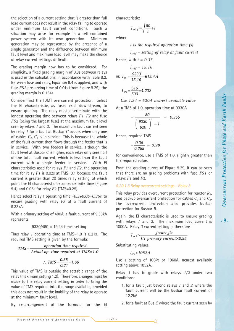
N e t w o r k P r o t e c t i o n & A u t o m a t i o n G u i d e • 1 4 5 •
the selection of a current setting that is greater than fullload current does not result in the relay failing to operateunder minimum fault current conditions. Such asituation may arise for example in a self-containedpower system with its own generation. Minimumgeneration may be represented by the presence of asingle generator and the difference between minimumfault level and maximum load level may make the choiceof relay current settings difficult.
The grading margin now has to be considered. Forsimplicity, a fixed grading margin of 0.3s between relaysis used in the calculations, in accordance with Table 9.2.Between fuse and relay, Equation 9.4 is applied, and withfuse FS2 pre-arcing time of 0.01s (from Figure 9.29), thegrading margin is 0.154s.
Consider first the IDMT overcurrent protection. Selectthe EI characteristic, as fuses exist downstream, toensure grading. The relay must discriminate with thelongest operating time between relays F1, F2 and fuseFS2 (being the largest fuse) at the maximum fault levelseen by relays 1 and 2. The maximum fault current seenby relay 1 for a fault at Busbar C occurs when only oneof cables C2, C3 is in service. This is because the wholeof the fault current then flows through the feeder that isin service. With two feeders in service, although thefault level at Busbar C is higher, each relay only sees halfof the total fault current, which is less than the faultcurrent with a single feeder in service. With EIcharacteristics used for relays F1 and F2, the operatingtime for relay F1 is 0.02s at TMS=0.1 because the faultcurrent is greater than 20 times relay setting, at whichpoint the EI characteristic becomes definite time (Figure9.4) and 0.05s for relay F2 (TMS=0.25).
Hence select relay 1 operating time =0.3+0.05=0.35s, toensure grading with relay F2 at a fault current of9.33kA.
With a primary setting of 480A, a fault current of 9.33kArepresents
9330/480 = 19.44 times setting
Thus relay 1 operating time at TMS=1.0 is 0.21s. Therequired TMS setting is given by the formula:
This value of TMS is outside the settable range of therelay (maximum setting 1.2). Therefore, changes must bemade to the relay current setting in order to bring thevalue of TMS required into the range available, providedthis does not result in the inability of the relay to operateat the minimum fault level.
By re-arrangement of the formula for the EI
∴ = = TMS 0 350 21
1 66..
.
TMS==
operation time requiredActual op. time required at TMS 1.0
characteristic:
where
t is the required operation time (s)
Isr1f = setting of relay at fault current
Hence, with t = 0.35,
Isr1f = 15.16
or,
Use 1.24 = 620A nearest available value
At a TMS of 1.0, operation time at 9330A
Hence, required TMS
for convenience, use a TMS of 1.0, slightly greater thanthe required value.
From the grading curves of Figure 9.29, it can be seenthat there are no grading problems with fuse FS1 orrelays F1 and F2.
9.20.1.5 Relay overcurrent settings - Relay 3
This relay provides overcurrent protection for reactor R1,and backup overcurrent protection for cables C2 and C3.The overcurrent protection also provides busbarprotection for Busbar B.
Again, the EI characteristic is used to ensure gradingwith relays 1 and 2. The maximum load current is1000A. Relay 3 current setting is therefore
Substituting values,
Isr3>1052A
Use a setting of 106% or 1060A, nearest availablesetting above 1052A.
Relay 3 has to grade with relays 1/2 under twoconditions:
1. for a fault just beyond relays 1 and 2 where thefault current will be the busbar fault current of12.2kA
2. for a fault at Bus C where the fault current seen by
I sr 3 0 95>
×feeder flc
CT primary current .
= =0 350 355
..
0.99
=⎛⎝⎜
⎞⎠⎟ −
=80
9330620
1
0 3552
.
I sr1616500
1 232= = .
I Asr19330
15 16615 4= =
..
Itsr f1
80 1= +
• 9 •O
verc
urre
nt P
rote
ctio
n fo
r Ph
ase
and
Ear
th F
aults
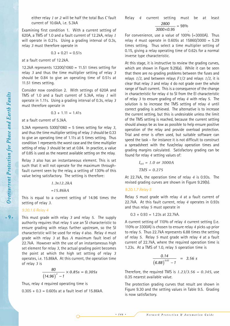
N e t w o r k P r o t e c t i o n & A u t o m a t i o n G u i d e
either relay 1 or 2 will be half the total Bus C faultcurrent of 10.6kA, i.e. 5.3kA
Examining first condition 1. With a current setting of620A, a TMS of 1.0 and a fault current of 12.2kA, relay 1will operate in 0.21s. Using a grading interval of 0.3s,relay 3 must therefore operate in
0.3 + 0.21 = 0.51s
at a fault current of 12.2kA.
12.2kA represents 12200/1060 = 11.51 times setting forrelay 3 and thus the time multiplier setting of relay 3should be 0.84 to give an operating time of 0.51s at11.51 times setting.
Consider now condition 2. With settings of 620A andTMS of 1.0 and a fault current of 5.3kA, relay 1 willoperate in 1.11s. Using a grading interval of 0.3s, relay 3must therefore operate in
0.3 + 1.11 = 1.41s
at a fault current of 5.3kA.
5.3kA represents 5300/1060 = 5 times setting for relay 3,and thus the time multiplier setting of relay 3 should be 0.33to give an operating time of 1.11s at 5 times setting. Thuscondition 1 represents the worst case and the time multipliersetting of relay 3 should be set at 0.84. In practice, a valueof 0.85 is used as the nearest available setting on the relay.
Relay 3 also has an instantaneous element. This is setsuch that it will not operate for the maximum through-fault current seen by the relay, a setting of 130% of thisvalue being satisfactory. The setting is therefore:
1.3x12.2kA
=15.86kA
This is equal to a current setting of 14.96 times thesetting of relay 3.
9.20.1.6 Relay 4
This must grade with relay 3 and relay 5. The supplyauthority requires that relay 5 use an SI characteristic toensure grading with relays further upstream, so the SIcharacteristic will be used for relay 4 also. Relay 4 mustgrade with relay 3 at Bus A maximum fault level of22.7kA. However with the use of an instantaneous highset element for relay 3, the actual grading point becomesthe point at which the high set setting of relay 3operates, i.e. 15.86kA. At this current, the operation timeof relay 3 is
Thus, relay 4 required operating time is
0.305 + 0.3 = 0.605s at a fault level of 15.86kA.
80
14 96 12
.( ) −× =0.85s 0.305s
Relay 4 current setting must be at least
= 98%.
For convenience, use a value of 100% (=3000A). Thusrelay 4 must operate in 0.605s at 15860/3000 = 5.29times setting. Thus select a time multiplier setting of0.15, giving a relay operating time of 0.62s for a normalinverse type characteristic.
At this stage, it is instructive to review the grading curves,which are shown in Figure 9.29(a). While it can be seenthat there are no grading problems between the fuses andrelays 1/2, and between relays F1/2 and relays 1/2, it isclear that relay 3 and relay 4 do not grade over the wholerange of fault current. This is a consequence of the changein characteristic for relay 4 to SI from the EI characteristicof relay 3 to ensure grading of relay 4 with relay 5. Thesolution is to increase the TMS setting of relay 4 untilcorrect grading is achieved. The alternative is to increasethe current setting, but this is undesirable unless the limitof the TMS setting is reached, because the current settingshould always be as low as possible to help ensure positiveoperation of the relay and provide overload protection.Trial and error is often used, but suitable software canspeed the task – for instance it is not difficult to constructa spreadsheet with the fuse/relay operation times andgrading margins calculated. Satisfactory grading can befound for relay 4 setting values of:
Ist4 = 1.0 or 3000A
TMS = 0.275
At 22.7kA, the operation time of relay 4 is 0.93s. Therevised grading curves are shown in Figure 9.29(b).
9.20.1.7 Relay 5
Relay 5 must grade with relay 4 at a fault current of22.7kA. At this fault current, relay 4 operates in 0.93sand thus relay 5 must operate in
0.3 + 0.93 = 1.23s at 22.7kA.
A current setting of 110% of relay 4 current setting (i.e.110% or 3300A) is chosen to ensure relay 4 picks up priorto relay 5. Thus 22.7kA represents 6.88 times the settingof relay 5. Relay 5 must grade with relay 4 at a faultcurrent of 22.7kA, where the required operation time is1.23s. At a TMS of 1.0, relay 5 operation time is
Therefore, the required TMS is 1.23/3.56 = 0.345, use0.35 nearest available value.
The protection grading curves that result are shown inFigure 9.30 and the setting values in Table 9.5. Gradingis now satisfactory.
0 14
6 88 13
0 02
.
..( ) −
= .56 s
28003000 0 95× .
• 9 •
Ove
rcur
rent
Pro
tect
ion
for
Phas
e an
d E
arth
Fau
lts
• 1 4 6 •
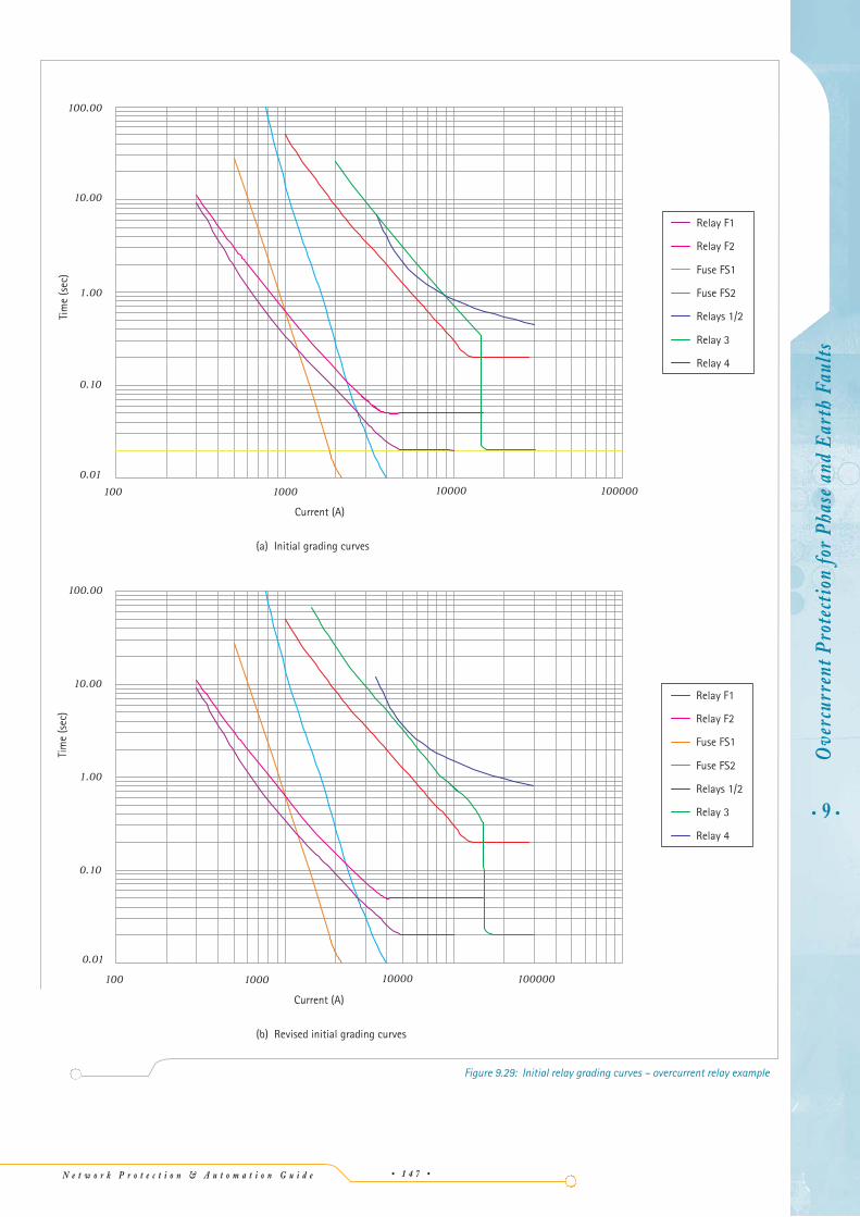
N e t w o r k P r o t e c t i o n & A u t o m a t i o n G u i d e • 1 4 7 •
• 9 •O
verc
urre
nt P
rote
ctio
n fo
r Ph
ase
and
Ear
th F
aults
0.01
0.10
1.00
10.00
100.00
100 1000 10000 100000
Current (A)
Tim
e (s
ec)
Relay F1
Relay F2
Fuse FS1
Fuse FS2
Relays 1/2
Relay 3
Relay 4
(a) Initial grading curves
0.01
0.10
1.00
10.00
100.00
100 1000 10000 100000
Current (A)
Tim
e (s
ec)
Relay F1
Relay F2
Fuse FS1
Fuse FS2
Relays 1/2
Relay 3
Relay 4
(b) Revised initial grading curves
Figure 9.29: Initial relay grading curves – overcurrent relay example
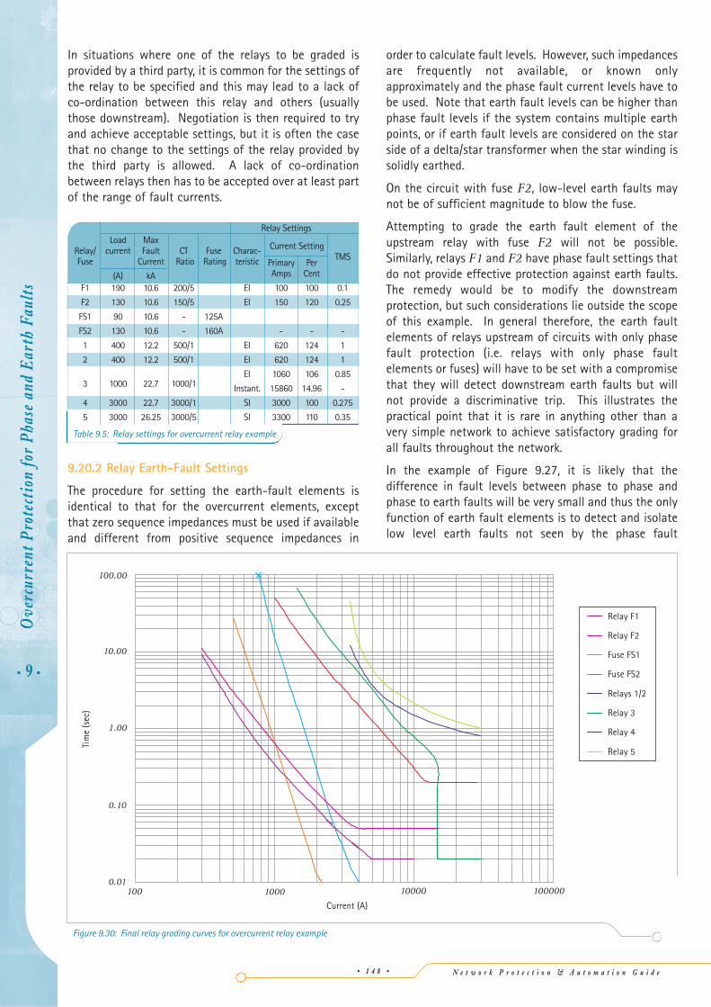
order to calculate fault levels. However, such impedancesare frequently not available, or known onlyapproximately and the phase fault current levels have tobe used. Note that earth fault levels can be higher thanphase fault levels if the system contains multiple earthpoints, or if earth fault levels are considered on the starside of a delta/star transformer when the star winding issolidly earthed.
On the circuit with fuse F2, low-level earth faults maynot be of sufficient magnitude to blow the fuse.
Attempting to grade the earth fault element of theupstream relay with fuse F2 will not be possible.Similarly, relays F1 and F2 have phase fault settings thatdo not provide effective protection against earth faults.The remedy would be to modify the downstreamprotection, but such considerations lie outside the scopeof this example. In general therefore, the earth faultelements of relays upstream of circuits with only phasefault protection (i.e. relays with only phase faultelements or fuses) will have to be set with a compromisethat they will detect downstream earth faults but willnot provide a discriminative trip. This illustrates thepractical point that it is rare in anything other than avery simple network to achieve satisfactory grading forall faults throughout the network.
In the example of Figure 9.27, it is likely that thedifference in fault levels between phase to phase andphase to earth faults will be very small and thus the onlyfunction of earth fault elements is to detect and isolatelow level earth faults not seen by the phase fault
Relay SettingsLoad Max
Current SettingRelay/ current Fault CT Fuse Charac-Fuse Current Ratio Rating teristic Primary Per
TMS
(A) kA Amps Cent
F1 190 10.6 200/5 EI 100 100 0.1
F2 130 10.6 150/5 EI 150 120 0.25
FS1 90 10.6 - 125A
FS2 130 10.6 - 160A - - -
1 400 12.2 500/1 EI 620 124 1
2 400 12.2 500/1 EI 620 124 1
3 1000 22.7 1000/1EI 1060 106 0.85
Instant. 15860 14.96 -
4 3000 22.7 3000/1 SI 3000 100 0.275
5 3000 26.25 3000/5 SI 3300 110 0.35
In situations where one of the relays to be graded isprovided by a third party, it is common for the settings ofthe relay to be specified and this may lead to a lack ofco-ordination between this relay and others (usuallythose downstream). Negotiation is then required to tryand achieve acceptable settings, but it is often the casethat no change to the settings of the relay provided bythe third party is allowed. A lack of co-ordinationbetween relays then has to be accepted over at least partof the range of fault currents.
9.20.2 Relay Earth-Fault Settings
The procedure for setting the earth-fault elements isidentical to that for the overcurrent elements, exceptthat zero sequence impedances must be used if availableand different from positive sequence impedances in
• 9 •
Ove
rcur
rent
Pro
tect
ion
for
Phas
e an
d E
arth
Fau
lts
Table 9.5: Relay settings for overcurrent relay example
0.01
0.10
1.00
10.00
100.00
100 1000 10000 100000
Current (A)
Tim
e (s
ec)
Relay F1
Relay F2
Fuse FS1
Fuse FS2
Relays 1/2
Relay 3
Relay 4
Relay 5
Figure 9.30: Final relay grading curves for overcurrent relay example
N e t w o r k P r o t e c t i o n & A u t o m a t i o n G u i d e• 1 4 8 •
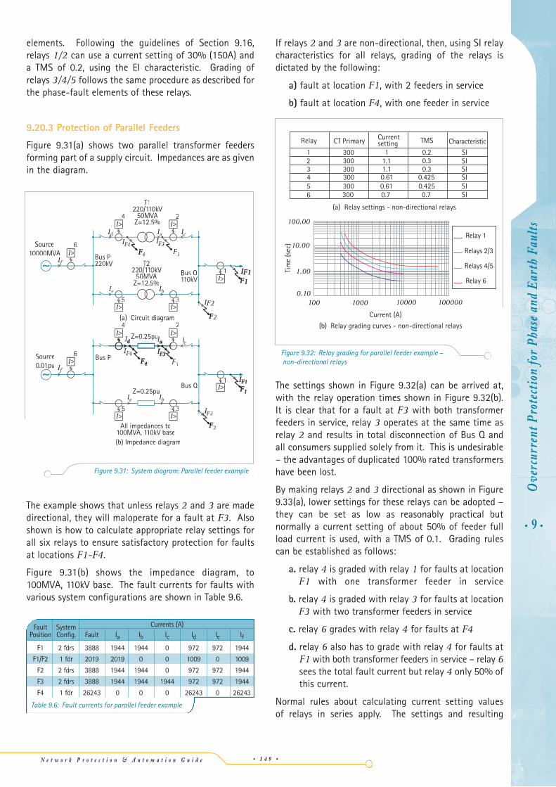
N e t w o r k P r o t e c t i o n & A u t o m a t i o n G u i d e • 1 4 9 •
elements. Following the guidelines of Section 9.16,relays 1/2 can use a current setting of 30% (150A) anda TMS of 0.2, using the EI characteristic. Grading ofrelays 3/4/5 follows the same procedure as described forthe phase-fault elements of these relays.
9.20.3 Protection of Parallel Feeders
Figure 9.31(a) shows two parallel transformer feedersforming part of a supply circuit. Impedances are as givenin the diagram.
The example shows that unless relays 2 and 3 are madedirectional, they will maloperate for a fault at F3. Alsoshown is how to calculate appropriate relay settings forall six relays to ensure satisfactory protection for faultsat locations F1-F4.
Figure 9.31(b) shows the impedance diagram, to100MVA, 110kV base. The fault currents for faults withvarious system configurations are shown in Table 9.6.
If relays 2 and 3 are non-directional, then, using SI relaycharacteristics for all relays, grading of the relays isdictated by the following:
a) fault at location F1, with 2 feeders in service
b) fault at location F4, with one feeder in service
The settings shown in Figure 9.32(a) can be arrived at,with the relay operation times shown in Figure 9.32(b).It is clear that for a fault at F3 with both transformerfeeders in service, relay 3 operates at the same time asrelay 2 and results in total disconnection of Bus Q andall consumers supplied solely from it. This is undesirable– the advantages of duplicated 100% rated transformershave been lost.
By making relays 2 and 3 directional as shown in Figure9.33(a), lower settings for these relays can be adopted –they can be set as low as reasonably practical butnormally a current setting of about 50% of feeder fullload current is used, with a TMS of 0.1. Grading rulescan be established as follows:
a. relay 4 is graded with relay 1 for faults at locationF1 with one transformer feeder in service
b. relay 4 is graded with relay 3 for faults at locationF3 with two transformer feeders in service
c. relay 6 grades with relay 4 for faults at F4
d. relay 6 also has to grade with relay 4 for faults atF1 with both transformer feeders in service – relay 6sees the total fault current but relay 4 only 50% ofthis current.
Normal rules about calculating current setting valuesof relays in series apply. The settings and resulting
• 9 •O
verc
urre
nt P
rote
ctio
n fo
r Ph
ase
and
Ear
th F
aults
1
IeII IbII
I
IfII
I
3
Z=0.25puII
3
4 2
6Source0.01pu
Bus P
Bus Q
All impedances to100MVA, 110kV base
pp
(b) Impedance diagram
I>II
>
I>II
>
>II
I>III>II
I>III>II
T1
50MVAZ=12.5%
50MVAZ=12.5%
5 3
4 2
6
If fII
IeII b
aIF4I
F3FISource
10000MVA Bus P220k
Bus Q110kV
Figure 9.31: System diagram: Parallel feeder example
Fault System Currents (A)Position Config. Fault Ia Ib Ic Id Ie If
F1 2 fdrs 3888 1944 1944 0 972 972 1944
F1/F2 1 fdr 2019 2019 0 0 1009 0 1009
F2 2 fdrs 3888 1944 1944 0 972 972 1944
F3 2 fdrs 3888 1944 1944 1944 972 972 1944
F4 1 fdr 26243 0 0 0 26243 0 26243
Table 9.6: Fault currents for parallel feeder example
0.10
1.00
10.00
100.00
100 1000 10000 100000
Tim
e (s
ec)
Current settingRelay CT Primary TMS Characteristic
1234
6
300
300
300300300
0.61
0.70.7
1.11.11
0.4250.30.30.2 SI
SISISI
5 300 0.61 0.425 SISI
(a) Relay settings - non-directional relays
(b) Relay grading curves - non-directional relays
Current (A)
Relay 1
Relays 2/3
Relays 4/5
Relay 6
Figure 9.32: Relay grading for parallel feeder example –non-directional relays
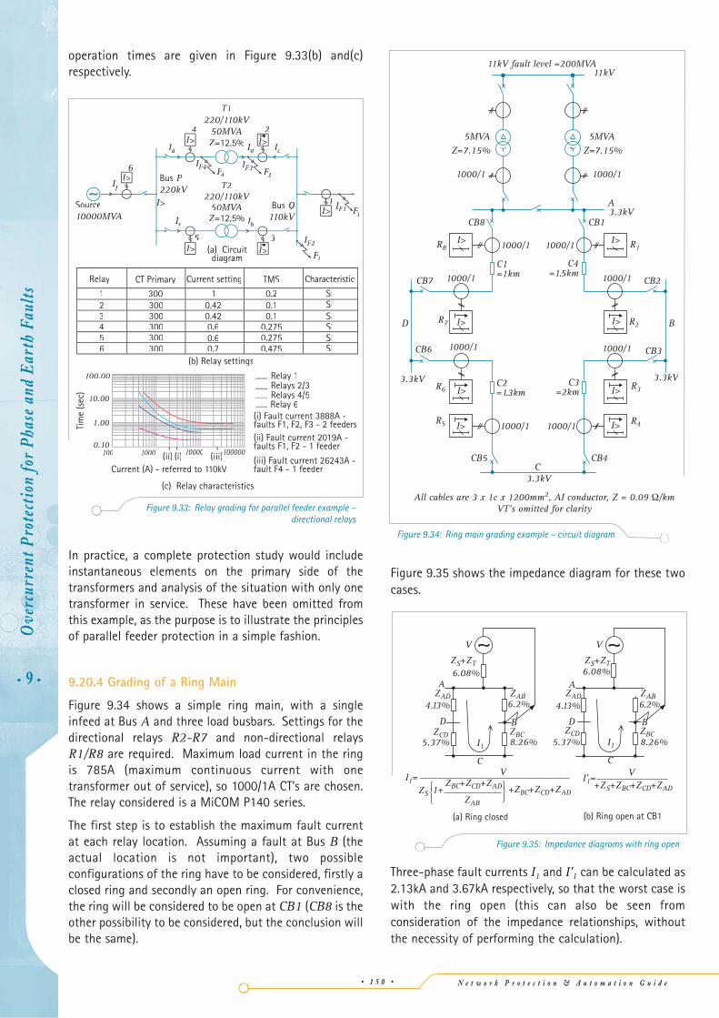
N e t w o r k P r o t e c t i o n & A u t o m a t i o n G u i d e
operation times are given in Figure 9.33(b) and(c)respectively.
In practice, a complete protection study would includeinstantaneous elements on the primary side of thetransformers and analysis of the situation with only onetransformer in service. These have been omitted fromthis example, as the purpose is to illustrate the principlesof parallel feeder protection in a simple fashion.
9.20.4 Grading of a Ring Main
Figure 9.34 shows a simple ring main, with a singleinfeed at Bus A and three load busbars. Settings for thedirectional relays R2-R7 and non-directional relaysR1/R8 are required. Maximum load current in the ringis 785A (maximum continuous current with onetransformer out of service), so 1000/1A CT’s are chosen.The relay considered is a MiCOM P140 series.
The first step is to establish the maximum fault currentat each relay location. Assuming a fault at Bus B (theactual location is not important), two possibleconfigurations of the ring have to be considered, firstly aclosed ring and secondly an open ring. For convenience,the ring will be considered to be open at CB1 (CB8 is theother possibility to be considered, but the conclusion willbe the same).
Figure 9.35 shows the impedance diagram for these twocases.
Three-phase fault currents I1 and I’1 can be calculated as2.13kA and 3.67kA respectively, so that the worst case iswith the ring open (this can also be seen fromconsideration of the impedance relationships, withoutthe necessity of performing the calculation).
• 9 •
Ove
rcur
rent
Pro
tect
ion
for
Phas
e an
d E
arth
Fau
lts
• 1 5 0 •
5MVAZ=7.15%
5MVAZ=7.15%
11kV fault level =200MVA11kV
C2=1.3km
CB5
CB6
CB8 CB1
R5
R6
R7 I>
R8 R1I> I>
R2I>
R3I>
R4I>I>
I>
CB4
C3=2km
C1=1km
C4=1.5km
1000/1
CB7 CB21000/1 1000/1
CB31000/1
1000/1 1000/1
1000/11000/1
3.3kV
D
1000/1
3.3kV
A3.3kV
3.3kV
B
1000/1
C
All cables are 3 x 1c x 1200mm2, AI conductor, Z = 0.09 Ω/kmVT's omitted for clarity
Figure 9.34: Ring main grading example – circuit diagram
diagram
T1
50MVAZ=12,5%
T2220/110kV
50MVAZ
5 3
4 2
1
6
IfI
IdII
IF4IF4FF
IF3IF3FF
F1 F1FF
IF2II
F2FF
e IbII
IaII IcII
Source10000MVA
Bus P220kV
Bus Q110kV
I>
I>
I>I>
I> I>
0.10
1.00
10.00
100.00
100 1000 (ii) (i) 10000
Current (A) - referred to 110kV
(i) Fault current 3888A -
faults F1, F2 - 1 feeder
(iii) Fault current 26243A -fault F4 - 1 feeder
Tim
e (s
ec)
Relay 1Relays 2/3Relays 4/5Relay 6
(c) Relay characteristics
(b) Relay settings
IFF
Relay CT Primary TMS Characteristic
123456
300
300300
300300300
0.6
0.70.6
0.420.42
1
0.275
0.4750.275
0.10.10.2 SI
SISISISISI
Current setting
(iii)
Figure 9.33: Relay grading for parallel feeder example –directional relays
(a) Ring closed
ZS+ZT
V
6.08%
ZCDI1
ZBC
D B
C
5.37% 8.26%
ZABZAD
A
4.13% 6.2%
I1=ZS
VZBC+ZCD+ZAD +ZBC+ZCD+ZAD
ZAB
⎧⎨⎩
⎧⎨⎩
1+
(b) Ring open at CB1
ZS+ZT
ZABZAD
ZCDI1
ZBC
A
D B
C
V
6.08%
4.13%
5.37% 8.26%
6.2%
I'1=V
+ZS+ZBC+ZCD+ZAD
Figure 9.35: Impedance diagrams with ring open
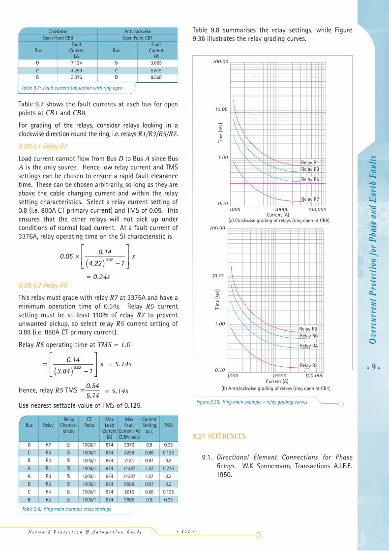
N e t w o r k P r o t e c t i o n & A u t o m a t i o n G u i d e • 1 5 1 •
Table 9.7 shows the fault currents at each bus for openpoints at CB1 and CB8.
For grading of the relays, consider relays looking in aclockwise direction round the ring, i.e. relays R1/R3/R5/R7.
9.20.4.1 Relay R7
Load current cannot flow from Bus D to Bus A since BusA is the only source. Hence low relay current and TMSsettings can be chosen to ensure a rapid fault clearancetime. These can be chosen arbitrarily, so long as they areabove the cable charging current and within the relaysetting characteristics. Select a relay current setting of0.8 (i.e. 800A CT primary current) and TMS of 0.05. Thisensures that the other relays will not pick up underconditions of normal load current. At a fault current of3376A, relay operating time on the SI characteristic is
= 0.24s9.20.4.2 Relay R5
This relay must grade with relay R7 at 3376A and have aminimum operation time of 0.54s. Relay R5 currentsetting must be at least 110% of relay R7 to preventunwanted pickup, so select relay R5 current setting of0.88 (i.e. 880A CT primary current).
Relay R5 operating time at TMS = 1.0
= 5.14s
Hence, relay R5 TMS = 5.14s
Use nearest settable value of TMS of 0.125.
= 0 545 14..
=( ) −
⎡
⎣⎢⎢
⎤
⎦⎥⎥
0 14
3 84 10 02
.
..
s
0 05 0 14
4 22 10 02
. .
..
×( ) −
⎡
⎣⎢⎢
⎤
⎦⎥⎥ s
Table 9.8 summarises the relay settings, while Figure9.36 illustrates the relay grading curves.
9.21 REFERENCES
9.1. Directional Element Connections for PhaseRelays. W.K Sonnemann, Transactions A.I.E.E.1950.
• 9 •O
verc
urre
nt P
rote
ctio
n fo
r Ph
ase
and
Ear
th F
aults
(a) Clockwise grading of relays (ring open at CB8)
10000.10
1.00
Current (A)10000 100,000
10.00
100.00
Tim
e (s
ec)
(b) Anticlockwise grading of relays (ring open at CB1)
100,0001000 10000Current (A)
0.10
1.00
10.00
100.00
Tim
e (s
ec)
yRelay R5
yyRelay R7
yRelay R2
Figure 9.36: Ring main example – relay grading curves
Clockwise AnticlockwiseOpen Point CB8 Open Point CB1
Fault FaultBus Current Bus Current
kA kAD 7.124 B 3.665
C 4.259 C 5.615B 3.376 D 8.568
Table 9.7: Fault current tabulation with ring open
Relay CT Max Max CurrentBus Relay Charact- Ratio Load Fault Setting TMS
eristic Current Current (A) p.u.(A) (3.3kV base)
D R7 SI 1000/1 874 3376 0.8 0.05
C R5 SI 1000/1 874 4259 0.88 0.125
B R3 SI 1000/1 874 7124 0.97 0.2
A R1 SI 1000/1 874 14387 1.07 0.275
A R8 SI 1000/1 874 14387 1.07 0.3
D R6 SI 1000/1 874 8568 0.97 0.2
C R4 SI 1000/1 874 5615 0.88 0.125
B R2 SI 1000/1 874 3665 0.8 0.05
Table 9.8: Ring main example relay settings