3,350+OPEN ACCESS BOOKS

108,000+INTERNATIONAL

AUTHORS AND EDITORS115+ MILLION

DOWNLOADS

BOOKSDELIVERED TO

151 COUNTRIES

AUTHORS AMONG

TOP 1%MOST CITED SCIENTIST

12.2%AUTHORS AND EDITORS

FROM TOP 500 UNIVERSITIES

Selection of our books indexed in theBook Citation Index in Web of Science™

Core Collection (BKCI)

Chapter from the book Air QualityDownloaded from: http://www.intechopen.com/books/air-quality

PUBLISHED BY

World's largest Science,Technology & Medicine

Open Access book publisher

Interested in publishing with IntechOpen?Contact us at book.department@intechopen.com

Estimation of uncertainty in predicting ground level concentrations from direct source releases in an urban area using the USEPA’s AERMOD model equations 169

Estimation of uncertainty in predicting ground level concentrations from direct source releases in an urban area using the USEPA’s AERMOD model equations

Vamsidhar V Poosarala, Ashok Kumar and Akhil Kadiyala

X

Estimation of uncertainty in predicting ground level concentrations from direct source

releases in an urban area using the USEPA’s AERMOD model equations

Vamsidhar V Poosarala, Ashok Kumar and Akhil Kadiyala

Department of Civil Engineering, The University of Toledo, Toledo, OH 43606

Abstract One of the important prerequisites for a model to be used in decision making is to perform uncertainty and sensitivity analyses on the outputs of the model. This study presents a comprehensive review of the uncertainty and sensitivity analyses associated with prediction of ground level pollutant concentrations using the USEPA’s AERMOD equations for point sources. This is done by first putting together an approximate set of equations that are used in the AERMOD model for the stable boundary layer (SBL) and convective boundary layer (CBL). Uncertainty and sensitivity analyses are then performed by incorporating the equations in Crystal Ball® software. Various parameters considered for these analyses include emission rate, stack exit velocity, stack exit temperature, wind speed, lateral dispersion parameter, vertical dispersion parameter, weighting coefficients for both updraft and downdraft, total horizontal distribution function, cloud cover, ambient temperature, and surface roughness length. The convective mixing height is also considered for the CBL cases because it was specified. The corresponding probability distribution functions, depending on the measured or practical values are assigned to perform uncertainty and sensitivity analyses in both CBL and SBL cases. The results for uncertainty in predicting ground level concentrations at different downwind distances in CBL varied between 67% and 75%, while it ranged between 40% and 47% in SBL. The sensitivity analysis showed that vertical dispersion parameter and total horizontal distribution function have contributed to 82% and 15% variance in predicting concentrations in CBL. In SBL, vertical dispersion parameter and total horizontal distribution function have contributed about 10% and 75% to variance in predicting concentrations respectively. Wind speed has a negative contribution to variance and the other parameters had a negligent or zero contribution to variance. The study concludes that the calculations of vertical dispersion parameter for the CBL case and of horizontal distribution function for the SBL case should be improved to reduce the uncertainty in predicting ground level concentrations.

8

www.intechopen.com

Air Quality170

1. Introduction Development of a good model for decision making in any field of study needs to be associated with uncertainty and sensitivity analyses. Performing uncertainty and sensitivity analyses on the output of a model is one of the basic prerequisites for model validation. Uncertainty can be defined as a measure of the ‘goodness’ of a result. One can perform uncertainty analysis to quantify the uncertainty associated with response of uncertainties in model input. Sensitivity analysis helps determine the variation in model output due to change in one or more input parameters for the model. Sensitivity analysis enables the modeler to rank the input parameters by their contribution to variance of the output and allows the modeler to determine the level of accuracy required for an input parameter to make the models sufficiently useful and valid. If one considers an input value to be varying from a standard existing value, then the person will be in a position to say by how much more or less sensitivity will the output be on comparing with the case of a standard existing value. By identifying the uncertainty and sensitivity of each model, a modeler gains the capability of making better decisions when considering more than one model to obtain desired accurate results. Hence, it is imperative for modelers to understand the importance of recording and understanding the uncertainty and sensitivity of each model developed that would assist industry and regulatory bodies in decision-making. A review of literature on the application of uncertainty and sensitivity analyses helped us gather some basic information on the applications of different methods in environmental area and their performance in computing uncertainty and sensitivity. The paper focuses on air quality modeling. Various stages at which uncertainty can be obtained are listed below.

a) Estimation of uncertainties in the model inputs. b) Estimation of the uncertainty in the results obtained from the model. c) Characterizing the uncertainties by different model structure and model formulations. d) Characterizing the uncertainties in model predicted results from the uncertainties in

evaluation data. Hanna (1988) stated the total uncertainty involved in modeling simulations to be considered as the sum of three components listed below.

a) Uncertainty due to errors in the model. b) Uncertainty due to errors in the input data. c) Uncertainty due to the stochastic processes in the atmosphere (like turbulence).

In order to estimate the uncertainty in predicting a variable using a model, the input parameters to which the model is more sensitive should be determined. This is referred to as sensitivity analysis, which indicates by how much the overall uncertainty in the model predictions is associated with the individual uncertainty of the inputs in the model [Vardoulakis et al. (2002)]. Sensitivity studies do not combine the uncertainty of the model inputs, to provide a realistic estimate of uncertainty of model output or results. Sensitivity analysis should be carried out for different variables of a model to decide where prominence should be placed in estimating the total uncertainty. Sensitivity analysis of dispersion parameters is useful, because, it promotes a deeper understanding of the phenomenon, and helps one in placing enough emphasis in accurate measurements of the variables. The analytical approach most frequently used for uncertainty analysis of simple equations is variance propagation [IAEA (1989), Martz and Waller (1982), Morgan and Henrion (1990)]. To overcome problems encountered with analytical variance propagation equations,

numerical methods are useful in performing an uncertainty analysis. Various approaches for determining uncertainty obtained from the literature include the following.

1) Differential uncertainty analysis [Cacuci (1981), and Worley (1987)] in which the partial derivatives of the model response with respect to the parameters are used to estimate uncertainty.

2) Monte Carlo analysis of statistical simplifications of complex models [Downing et al. (1985), Mead and Pike (1975), Morton (1983), and Myers (1971), Kumar et al. (1999)].

3) Non-probabilistic methods [for example: fuzzy sets, fuzzy arithmetic, and possibility theory [Ferson and Kuhn (1992)].

4) First-order analysis employing Taylor expansions [Scavia et al. (1981)]. 5) Bootstrap method [Romano et al. (2004)]. 6) Probability theory [Zadeh (1978)].

The most commonly applied numerical technique is the Monte Carlo simulation (Rubinstein, 1981). There are many methods by which sensitivity analysis can be performed. Some of the methods are listed below.

1) Simple regression (on the untransformed and transformed data) [Brenkert et al. (1988)] or visual analysis of output based on changes in input [(Kumar et al. (1987), Thomas et al. (1985), Kumar et al. (2008)].

2) Multiple and piecewise multiple regression (on transformed and untransformed data) [Downing et al. (1985)].

3) Regression coefficients and partial regression coefficients [Bartell et al. (1986), Gardner et al. (1981)].

4) Stepwise regression and correlation ratios (on untransformed and transformed data). 5) Differential sensitivity analysis [Griewank and Corliss (1991), Worley (1987)]. 6) Evidence theory [Dempster (1967), Shafer (1976)]. 7) Interval approaches (Hansen and Walster, 2002). 8) ASTM method [(Kumar et al. (2002), Patel et al. (2003)].

Other studies that discuss the use of statistical regressions of the randomly selected values of uncertain parameters on the values produced for model predictions to determine the importance of parameters contributing to the overall uncertainty in the model result include IAEA (1989), Iman et al. (1981a, 1981b), Iman and Helton (1991), and Morgan and Henrion (1990). Romano et al. (2004) performed the uncertainty analysis using Monte Carlo, Bootstrap, and fuzzy methods to determine the uncertainty associated with air emissions from two electric power plants in Italy. Emissions monitored were sulfur dioxide (SO2), nitrogen oxides (NOX), carbon monoxide (CO), and particulate matter (PM). Daily average emission data from a coal plant having two boilers were collected in 1998, and hourly average emission data from a fuel oil plant having four boilers were collected in 2000. The study compared the uncertainty analysis results from the three methods and concluded that Monte Carlo method gave more accurate results when applied to the Gaussian distributions, while Bootstrap method produced better results in estimating uncertainty for irregular and asymmetrical distributions, and Fuzzy models are well suited for cases where there is limited data availability or the data are not known properly. Int Panis et al. (2004) studied the parametric uncertainty of aggregating marginal external costs for all motorized road transportation modes to the national level air pollution in

www.intechopen.com

Estimation of uncertainty in predicting ground level concentrations from direct source releases in an urban area using the USEPA’s AERMOD model equations 171

1. Introduction Development of a good model for decision making in any field of study needs to be associated with uncertainty and sensitivity analyses. Performing uncertainty and sensitivity analyses on the output of a model is one of the basic prerequisites for model validation. Uncertainty can be defined as a measure of the ‘goodness’ of a result. One can perform uncertainty analysis to quantify the uncertainty associated with response of uncertainties in model input. Sensitivity analysis helps determine the variation in model output due to change in one or more input parameters for the model. Sensitivity analysis enables the modeler to rank the input parameters by their contribution to variance of the output and allows the modeler to determine the level of accuracy required for an input parameter to make the models sufficiently useful and valid. If one considers an input value to be varying from a standard existing value, then the person will be in a position to say by how much more or less sensitivity will the output be on comparing with the case of a standard existing value. By identifying the uncertainty and sensitivity of each model, a modeler gains the capability of making better decisions when considering more than one model to obtain desired accurate results. Hence, it is imperative for modelers to understand the importance of recording and understanding the uncertainty and sensitivity of each model developed that would assist industry and regulatory bodies in decision-making. A review of literature on the application of uncertainty and sensitivity analyses helped us gather some basic information on the applications of different methods in environmental area and their performance in computing uncertainty and sensitivity. The paper focuses on air quality modeling. Various stages at which uncertainty can be obtained are listed below.

a) Estimation of uncertainties in the model inputs. b) Estimation of the uncertainty in the results obtained from the model. c) Characterizing the uncertainties by different model structure and model formulations. d) Characterizing the uncertainties in model predicted results from the uncertainties in

evaluation data. Hanna (1988) stated the total uncertainty involved in modeling simulations to be considered as the sum of three components listed below.

a) Uncertainty due to errors in the model. b) Uncertainty due to errors in the input data. c) Uncertainty due to the stochastic processes in the atmosphere (like turbulence).

In order to estimate the uncertainty in predicting a variable using a model, the input parameters to which the model is more sensitive should be determined. This is referred to as sensitivity analysis, which indicates by how much the overall uncertainty in the model predictions is associated with the individual uncertainty of the inputs in the model [Vardoulakis et al. (2002)]. Sensitivity studies do not combine the uncertainty of the model inputs, to provide a realistic estimate of uncertainty of model output or results. Sensitivity analysis should be carried out for different variables of a model to decide where prominence should be placed in estimating the total uncertainty. Sensitivity analysis of dispersion parameters is useful, because, it promotes a deeper understanding of the phenomenon, and helps one in placing enough emphasis in accurate measurements of the variables. The analytical approach most frequently used for uncertainty analysis of simple equations is variance propagation [IAEA (1989), Martz and Waller (1982), Morgan and Henrion (1990)]. To overcome problems encountered with analytical variance propagation equations,

numerical methods are useful in performing an uncertainty analysis. Various approaches for determining uncertainty obtained from the literature include the following.

1) Differential uncertainty analysis [Cacuci (1981), and Worley (1987)] in which the partial derivatives of the model response with respect to the parameters are used to estimate uncertainty.

2) Monte Carlo analysis of statistical simplifications of complex models [Downing et al. (1985), Mead and Pike (1975), Morton (1983), and Myers (1971), Kumar et al. (1999)].

3) Non-probabilistic methods [for example: fuzzy sets, fuzzy arithmetic, and possibility theory [Ferson and Kuhn (1992)].

4) First-order analysis employing Taylor expansions [Scavia et al. (1981)]. 5) Bootstrap method [Romano et al. (2004)]. 6) Probability theory [Zadeh (1978)].

The most commonly applied numerical technique is the Monte Carlo simulation (Rubinstein, 1981). There are many methods by which sensitivity analysis can be performed. Some of the methods are listed below.

1) Simple regression (on the untransformed and transformed data) [Brenkert et al. (1988)] or visual analysis of output based on changes in input [(Kumar et al. (1987), Thomas et al. (1985), Kumar et al. (2008)].

2) Multiple and piecewise multiple regression (on transformed and untransformed data) [Downing et al. (1985)].

3) Regression coefficients and partial regression coefficients [Bartell et al. (1986), Gardner et al. (1981)].

4) Stepwise regression and correlation ratios (on untransformed and transformed data). 5) Differential sensitivity analysis [Griewank and Corliss (1991), Worley (1987)]. 6) Evidence theory [Dempster (1967), Shafer (1976)]. 7) Interval approaches (Hansen and Walster, 2002). 8) ASTM method [(Kumar et al. (2002), Patel et al. (2003)].

Other studies that discuss the use of statistical regressions of the randomly selected values of uncertain parameters on the values produced for model predictions to determine the importance of parameters contributing to the overall uncertainty in the model result include IAEA (1989), Iman et al. (1981a, 1981b), Iman and Helton (1991), and Morgan and Henrion (1990). Romano et al. (2004) performed the uncertainty analysis using Monte Carlo, Bootstrap, and fuzzy methods to determine the uncertainty associated with air emissions from two electric power plants in Italy. Emissions monitored were sulfur dioxide (SO2), nitrogen oxides (NOX), carbon monoxide (CO), and particulate matter (PM). Daily average emission data from a coal plant having two boilers were collected in 1998, and hourly average emission data from a fuel oil plant having four boilers were collected in 2000. The study compared the uncertainty analysis results from the three methods and concluded that Monte Carlo method gave more accurate results when applied to the Gaussian distributions, while Bootstrap method produced better results in estimating uncertainty for irregular and asymmetrical distributions, and Fuzzy models are well suited for cases where there is limited data availability or the data are not known properly. Int Panis et al. (2004) studied the parametric uncertainty of aggregating marginal external costs for all motorized road transportation modes to the national level air pollution in

www.intechopen.com

Air Quality172

Belgium using the Monte Carlo technique. This study uses the impact pathway methodology that involves basically following a pollutant from its emission until it causes an impact or damage. The methodology involves details on the generation of emissions, atmospheric dispersion, exposure of humans and environment to pollutants, and impacts on public health, agriculture, and buildings. The study framework involves a combination of emission models, and air dispersion models at local and regional scales with dose-response functions and valuation rules. The propagation of errors was studied through complex calculations and the error estimates of every parameter used for the calculation were replaced by probability distribution. The above procedure is repeated many times (between 1000 and 10,000 trails) so that a large number of combinations of different input parameters occur. For this analysis, all the calculations were performed using the Crystal Ball® software. Based on the sensitivity of the result, parameters that contributed more to the variations were determined and studied in detail to obtain a better estimate of the parameter. The study observed the fraction high-emitter diesel passenger cars, air conditioning, and the impacts of foreign trucks as the main factors contributing to uncertainty for 2010 estimate. Sax and Isakov (2003) have estimated the contribution of variability and uncertainty in the Gaussian air pollutant dispersion modeling systems from four model components: emissions, spatial and temporal allocation of emissions, model parameters, and meteorology using Monte Carlo simulations across ISCST3 and AERMOD. Variability and uncertainty in predicted hexavalent chromium concentrations generated from welding operations were studied. Results showed that a 95 percent confidence interval of predicted pollutant concentrations varied in magnitude at each receptor indicating that uncertainty played an important role at the receptors. AERMOD predicted a greater range of pollutant concentration as compared to ISCST3 for low-level sources in this study. The conclusion of the study was that input parameters need to be well characterized to reduce the uncertainty. Rodriguez et al. (2007) investigated the uncertainty and sensitivity of ozone and PM2.5 aerosols to variations in selected input parameters using a Monte Carlo analysis. The input parameters were selected based on their potential in affecting the pollutant concentrations predicted by the model and changes in emissions due to distributed generation (DG) implementation in the South Coast Air Basin (SoCAB) of California. Numerical simulations were performed using CIT three-dimensional air quality model. The magnitudes of the largest impacts estimated in this study are greater and well beyond the contribution of emissions uncertainty to the estimated air quality model error. Emissions introduced by DG implementation produce a highly non-linear response in time and space on pollutant concentrations. Results also showed that concentrating DG emissions in space or time produced the largest air quality impacts in the SoCAB area. Thus, in addition to the total amount of possible distributed generation to be installed, regulators should also consider the type of DG installed (as well as their spatial distribution) to avoid undesirable air quality impacts. After performing the sensitivity analysis, it was observed from the study that the current model is good enough to predict the air quality impacts of DG emissions as long as the changes in ozone are greater than 5 ppb and changes in PM2.5 are greater than 13µg/m3. Hwang et al. (1998) analyzed and discussed the techniques for model sensitivity and uncertainty analyses, and analysis of the propagation of model uncertainty for the model used within the GIS environment. A two-dimensional air quality model based on the first order Taylor method was used in this study. The study observed brute force method, the most straightforward method for sensitivity to be providing approximate solutions with

substantial human efforts. On the other hand, automatic differentiation required only one model run with minimum human effort to compute the solution where results are accurate to the precision of the machine. The study also observed that sampling methods provide only partial information with unknown accuracy while first-order method combined with automatic differentiation provide a complete solution with known accuracy. These techniques can be used for any model that is first order differentiable. Rao (2005) has discussed various types of uncertainties in the atmospheric dispersion models and reviewed sensitivity and uncertainty analysis methods to characterize and/or reduce them. This study concluded the results based on the confidence intervals (CI). If 5% of CI for pollutant concentration is less than that of the regulatory standards, then remedial measures must be taken. If the CI is more than 95% of the regulatory standards, nothing needs to be done. If the 95% upper CI is above the standard and the 50th percentile is below, further study must be carried out on the important parameters which play a key role in calculation of the concentration value. If the 50th percentile is also above the standard, one can proceed with cost effective remedial measures for risk reduction even though more study needs to be carried out. The study concluded that the uncertainty analysis incorporated into the atmospheric dispersion models would be valuable in decision-making. Yegnan et al. (2002) demonstrated the need of incorporating uncertainty in dispersion models by applying uncertainty to two critical input parameters (wind speed and ambient temperature) in calculating the ground level concentrations. In this study, the Industrial Source Complex Short Term (ISCST) model, which is a Gaussian dispersion model, is used to predict the pollutant transport from a point source and the first-order and second-order Taylor series are used to calculate the ground level uncertainties. The results of ISCST model and uncertainty calculations are then validated with Monte Carlo simulations. There was a linear relationship between inputs and output. From the results, it was observed that the first-order Taylor series have been appropriate for ambient temperature and the second-order series is appropriate for wind speed when compared to Monte Carlo method. Gottschalk et al. (2007) tested the uncertainty associated with simulation of NEE (net ecosystem exchange) by the PaSim (pasture simulation model) at four grassland sites. Monte Carlo runs were performed for the years 2002 and 2003, using Latin Hypercube sampling from probability density functions (PDF) for each input factor to know the effect of measurement uncertainties in the main input factors like climate, atmospheric CO2 concentrations, soil characteristics, and management. This shows that output uncertainty not only depends on the input uncertainty, but also depends on the important factors and the uncertainty in model simulations. The study concluded that if a system is more environmentally confined, there will be higher uncertainties in the model results. In addition to the above mentioned studies, many studies have focused on assessing the uncertainty in air quality models [Freeman et al. (1986), Seigneur et al. (1992), Hanna et al. (1998, 2001), Bergin et al. (1999), Yang et al. (1997), Moore and Londergan (2001), Hanna and Davis (2002), Vardoulakis et al. (2002), Hakami et al. (2003), Jaarsveld et al. (1997), Smith et al. (2000), and Guensler and Leonard (1995)]. Derwent and Hov (1988), Gao et al. (1996), Phenix et al. (1998), Bergin et al. (1999), Grenfell et al. (1999), Hanna et al. (2001), and Vuilleumier et al. (2001) have used the Monte Carlo simulations to address uncertainty in regional-scale gas-phase mechanisms. Uncertainty in meteorology inputs was studied by Irwin et al. (1987), and Dabberdt and Miller (2000), while the uncertainty in emissions was observed by Frey and Rhodes (1996), Frey and Li (2002), and Frey and Zheng (2002).

www.intechopen.com

Estimation of uncertainty in predicting ground level concentrations from direct source releases in an urban area using the USEPA’s AERMOD model equations 173

Belgium using the Monte Carlo technique. This study uses the impact pathway methodology that involves basically following a pollutant from its emission until it causes an impact or damage. The methodology involves details on the generation of emissions, atmospheric dispersion, exposure of humans and environment to pollutants, and impacts on public health, agriculture, and buildings. The study framework involves a combination of emission models, and air dispersion models at local and regional scales with dose-response functions and valuation rules. The propagation of errors was studied through complex calculations and the error estimates of every parameter used for the calculation were replaced by probability distribution. The above procedure is repeated many times (between 1000 and 10,000 trails) so that a large number of combinations of different input parameters occur. For this analysis, all the calculations were performed using the Crystal Ball® software. Based on the sensitivity of the result, parameters that contributed more to the variations were determined and studied in detail to obtain a better estimate of the parameter. The study observed the fraction high-emitter diesel passenger cars, air conditioning, and the impacts of foreign trucks as the main factors contributing to uncertainty for 2010 estimate. Sax and Isakov (2003) have estimated the contribution of variability and uncertainty in the Gaussian air pollutant dispersion modeling systems from four model components: emissions, spatial and temporal allocation of emissions, model parameters, and meteorology using Monte Carlo simulations across ISCST3 and AERMOD. Variability and uncertainty in predicted hexavalent chromium concentrations generated from welding operations were studied. Results showed that a 95 percent confidence interval of predicted pollutant concentrations varied in magnitude at each receptor indicating that uncertainty played an important role at the receptors. AERMOD predicted a greater range of pollutant concentration as compared to ISCST3 for low-level sources in this study. The conclusion of the study was that input parameters need to be well characterized to reduce the uncertainty. Rodriguez et al. (2007) investigated the uncertainty and sensitivity of ozone and PM2.5 aerosols to variations in selected input parameters using a Monte Carlo analysis. The input parameters were selected based on their potential in affecting the pollutant concentrations predicted by the model and changes in emissions due to distributed generation (DG) implementation in the South Coast Air Basin (SoCAB) of California. Numerical simulations were performed using CIT three-dimensional air quality model. The magnitudes of the largest impacts estimated in this study are greater and well beyond the contribution of emissions uncertainty to the estimated air quality model error. Emissions introduced by DG implementation produce a highly non-linear response in time and space on pollutant concentrations. Results also showed that concentrating DG emissions in space or time produced the largest air quality impacts in the SoCAB area. Thus, in addition to the total amount of possible distributed generation to be installed, regulators should also consider the type of DG installed (as well as their spatial distribution) to avoid undesirable air quality impacts. After performing the sensitivity analysis, it was observed from the study that the current model is good enough to predict the air quality impacts of DG emissions as long as the changes in ozone are greater than 5 ppb and changes in PM2.5 are greater than 13µg/m3. Hwang et al. (1998) analyzed and discussed the techniques for model sensitivity and uncertainty analyses, and analysis of the propagation of model uncertainty for the model used within the GIS environment. A two-dimensional air quality model based on the first order Taylor method was used in this study. The study observed brute force method, the most straightforward method for sensitivity to be providing approximate solutions with

substantial human efforts. On the other hand, automatic differentiation required only one model run with minimum human effort to compute the solution where results are accurate to the precision of the machine. The study also observed that sampling methods provide only partial information with unknown accuracy while first-order method combined with automatic differentiation provide a complete solution with known accuracy. These techniques can be used for any model that is first order differentiable. Rao (2005) has discussed various types of uncertainties in the atmospheric dispersion models and reviewed sensitivity and uncertainty analysis methods to characterize and/or reduce them. This study concluded the results based on the confidence intervals (CI). If 5% of CI for pollutant concentration is less than that of the regulatory standards, then remedial measures must be taken. If the CI is more than 95% of the regulatory standards, nothing needs to be done. If the 95% upper CI is above the standard and the 50th percentile is below, further study must be carried out on the important parameters which play a key role in calculation of the concentration value. If the 50th percentile is also above the standard, one can proceed with cost effective remedial measures for risk reduction even though more study needs to be carried out. The study concluded that the uncertainty analysis incorporated into the atmospheric dispersion models would be valuable in decision-making. Yegnan et al. (2002) demonstrated the need of incorporating uncertainty in dispersion models by applying uncertainty to two critical input parameters (wind speed and ambient temperature) in calculating the ground level concentrations. In this study, the Industrial Source Complex Short Term (ISCST) model, which is a Gaussian dispersion model, is used to predict the pollutant transport from a point source and the first-order and second-order Taylor series are used to calculate the ground level uncertainties. The results of ISCST model and uncertainty calculations are then validated with Monte Carlo simulations. There was a linear relationship between inputs and output. From the results, it was observed that the first-order Taylor series have been appropriate for ambient temperature and the second-order series is appropriate for wind speed when compared to Monte Carlo method. Gottschalk et al. (2007) tested the uncertainty associated with simulation of NEE (net ecosystem exchange) by the PaSim (pasture simulation model) at four grassland sites. Monte Carlo runs were performed for the years 2002 and 2003, using Latin Hypercube sampling from probability density functions (PDF) for each input factor to know the effect of measurement uncertainties in the main input factors like climate, atmospheric CO2 concentrations, soil characteristics, and management. This shows that output uncertainty not only depends on the input uncertainty, but also depends on the important factors and the uncertainty in model simulations. The study concluded that if a system is more environmentally confined, there will be higher uncertainties in the model results. In addition to the above mentioned studies, many studies have focused on assessing the uncertainty in air quality models [Freeman et al. (1986), Seigneur et al. (1992), Hanna et al. (1998, 2001), Bergin et al. (1999), Yang et al. (1997), Moore and Londergan (2001), Hanna and Davis (2002), Vardoulakis et al. (2002), Hakami et al. (2003), Jaarsveld et al. (1997), Smith et al. (2000), and Guensler and Leonard (1995)]. Derwent and Hov (1988), Gao et al. (1996), Phenix et al. (1998), Bergin et al. (1999), Grenfell et al. (1999), Hanna et al. (2001), and Vuilleumier et al. (2001) have used the Monte Carlo simulations to address uncertainty in regional-scale gas-phase mechanisms. Uncertainty in meteorology inputs was studied by Irwin et al. (1987), and Dabberdt and Miller (2000), while the uncertainty in emissions was observed by Frey and Rhodes (1996), Frey and Li (2002), and Frey and Zheng (2002).

www.intechopen.com

Air Quality174

Seigneur et al. (1992), Frey (1993), and Cullen and Frey (1999) have assessed the uncertainty for a health risk assessment. From the literature review, it was observed that uncertainty and sensitivity analyses have been carried out for various cases having different model parameters for varying emissions inventories, air pollutants, air quality modeling, and dispersion models. However, only one of these studies [Sax and Isakov (2003)] reported in the literature discussed such application of uncertainty and sensitivity analyses for predicting ground level concentrations using AERMOD equations. This study tries to fill this knowledge gap by performing uncertainty and sensitivity analyses of the results obtained at ground level from the AERMOD equations using urban area emission data with Crystal Ball® software.

2. Methodology This section provides a detailed overview of the various steps adopted by the researchers when performing uncertainty and sensitivity analyses over predicted ground level pollutant concentrations from a point source in an urban area using the United States Environmental Protection Agency’s (U.S. EPA’s) AERMOD equations. The study focuses on determining the uncertainty in predicting ground level pollutant concentrations using the AERMOD equations.

2.1 AERMOD Spreadsheet Development The researchers put together an approximate set of equations that are used in the AERMOD model for the stable boundary layer (SBL) and convective boundary layer (CBL). Note that the AERMOD model treats atmospheric conditions either as stable or convective. The basic equations used for calculating concentrations in both CBL and SBL are programmed in a spreadsheet. The following is a list of assumptions used while deriving the parameters and choosing the concentration equations in both SBL and CBL.

1) Only direct source equation is taken to calculate the pollutant concentration in CBL. However, there is only one equation for all conditions in the stable boundary layer.

2) The fraction of plume mass concentration in CBL is taken as one. This assumes that the plume will not penetrate the convective boundary layer at any point during dispersion and plume is dispersing within the CBL.

3) The value of convective mixing height is taken by assuming a value for each hour i.e., it is not computed using the equations given in the AERMOD manual.

2.1.1 Stable Boundary Layer (SBL) and Convective Boundary Layer (CBL) Equations This section presents the AERMOD model equations that are incorporated in to the AERMOD spreadsheet for stable and convective boundary layer conditions.

2.1.1a Concentration Calculations in the SBL and CBL* For stable boundary conditions, the AERMOD concentration expression (Cs in equation 1a) has the Gaussian form, and is similar to that used in many other steady-state plume models. The equation for Cs is given by,

(1a)

For the case of m = 1 (i.e. m= -1, 0, 1), the above equation changes to the form of equation 1b.

(1b) The equation for calculation of the pollutant concentration in the convective boundary layer is given by equation 2a.

(2a) for m = 1 (i.e. m= 0, 1) the above equations changes to the form of equation 2b.

(2b)

* The symbols are explained in the Nomenclature section at the end of the Chapter.

2.1.1b Friction Velocity (u*) in SBL and CBL The computation of friction velocity (u*) under SBL conditions is given by equation 3.

(3)

where, [Hanna and Chang (1993), Perry (1992)] (4)

[Garratt (1992)] (5)

www.intechopen.com

Estimation of uncertainty in predicting ground level concentrations from direct source releases in an urban area using the USEPA’s AERMOD model equations 175

Seigneur et al. (1992), Frey (1993), and Cullen and Frey (1999) have assessed the uncertainty for a health risk assessment. From the literature review, it was observed that uncertainty and sensitivity analyses have been carried out for various cases having different model parameters for varying emissions inventories, air pollutants, air quality modeling, and dispersion models. However, only one of these studies [Sax and Isakov (2003)] reported in the literature discussed such application of uncertainty and sensitivity analyses for predicting ground level concentrations using AERMOD equations. This study tries to fill this knowledge gap by performing uncertainty and sensitivity analyses of the results obtained at ground level from the AERMOD equations using urban area emission data with Crystal Ball® software.

2. Methodology This section provides a detailed overview of the various steps adopted by the researchers when performing uncertainty and sensitivity analyses over predicted ground level pollutant concentrations from a point source in an urban area using the United States Environmental Protection Agency’s (U.S. EPA’s) AERMOD equations. The study focuses on determining the uncertainty in predicting ground level pollutant concentrations using the AERMOD equations.

2.1 AERMOD Spreadsheet Development The researchers put together an approximate set of equations that are used in the AERMOD model for the stable boundary layer (SBL) and convective boundary layer (CBL). Note that the AERMOD model treats atmospheric conditions either as stable or convective. The basic equations used for calculating concentrations in both CBL and SBL are programmed in a spreadsheet. The following is a list of assumptions used while deriving the parameters and choosing the concentration equations in both SBL and CBL.

1) Only direct source equation is taken to calculate the pollutant concentration in CBL. However, there is only one equation for all conditions in the stable boundary layer.

2) The fraction of plume mass concentration in CBL is taken as one. This assumes that the plume will not penetrate the convective boundary layer at any point during dispersion and plume is dispersing within the CBL.

3) The value of convective mixing height is taken by assuming a value for each hour i.e., it is not computed using the equations given in the AERMOD manual.

2.1.1 Stable Boundary Layer (SBL) and Convective Boundary Layer (CBL) Equations This section presents the AERMOD model equations that are incorporated in to the AERMOD spreadsheet for stable and convective boundary layer conditions.

2.1.1a Concentration Calculations in the SBL and CBL* For stable boundary conditions, the AERMOD concentration expression (Cs in equation 1a) has the Gaussian form, and is similar to that used in many other steady-state plume models. The equation for Cs is given by,

(1a)

For the case of m = 1 (i.e. m= -1, 0, 1), the above equation changes to the form of equation 1b.

(1b) The equation for calculation of the pollutant concentration in the convective boundary layer is given by equation 2a.

(2a) for m = 1 (i.e. m= 0, 1) the above equations changes to the form of equation 2b.

(2b)

* The symbols are explained in the Nomenclature section at the end of the Chapter.

2.1.1b Friction Velocity (u*) in SBL and CBL The computation of friction velocity (u*) under SBL conditions is given by equation 3.

(3)

where, [Hanna and Chang (1993), Perry (1992)] (4)

[Garratt (1992)] (5)

www.intechopen.com

Air Quality176

Substituting equations 4 and 5 in equation 3, one gets the equation of friction velocity, u* for SBL conditions, as given by equation 6.

(6)

The computation of friction velocity u* under CBL conditions is given by equation 7.

(7)

2.1.1c Effective Stack Height in SBL The effective stack height (hes) is given by equation 8.

(8) where, Δhs is calculated by using equation 9.

(9)

where, N’=0.7N,

(10)

(K m-1) is potential temperature gradient.

(11)

(12)

2.1.1d Height of the Reflecting Surface in SBL The height of reflecting surface in stable boundary layer is computed using equation 13.

(13)

where,

(14)

(15)

(16)

[Venkatram et.al., 1984] (17)

ln = 0.36.hes and ls = 0.27. ( ), zi = zim.

2.1.1e Total Height of the Direct Source Plume in CBL The actual height of the direct source plume will be the combination of the release height, buoyancy, and convection. The equation for total height of the direct source plume is given by equation 18.

(18)

(19)

wj = aj.w* where, subscript j is equal to 1 for updrafts and 2 for the downdrafts. λj in equation 2 is given by λ1 and λ2 for updraft and downdraft respectively and they are calculated using equations 20 and 21 respectively.

(20)

(21)

www.intechopen.com

Estimation of uncertainty in predicting ground level concentrations from direct source releases in an urban area using the USEPA’s AERMOD model equations 177

Substituting equations 4 and 5 in equation 3, one gets the equation of friction velocity, u* for SBL conditions, as given by equation 6.

(6)

The computation of friction velocity u* under CBL conditions is given by equation 7.

(7)

2.1.1c Effective Stack Height in SBL The effective stack height (hes) is given by equation 8.

(8) where, Δhs is calculated by using equation 9.

(9)

where, N’=0.7N,

(10)

(K m-1) is potential temperature gradient.

(11)

(12)

2.1.1d Height of the Reflecting Surface in SBL The height of reflecting surface in stable boundary layer is computed using equation 13.

(13)

where,

(14)

(15)

(16)

[Venkatram et.al., 1984] (17)

ln = 0.36.hes and ls = 0.27. ( ), zi = zim.

2.1.1e Total Height of the Direct Source Plume in CBL The actual height of the direct source plume will be the combination of the release height, buoyancy, and convection. The equation for total height of the direct source plume is given by equation 18.

(18)

(19)

wj = aj.w* where, subscript j is equal to 1 for updrafts and 2 for the downdrafts. λj in equation 2 is given by λ1 and λ2 for updraft and downdraft respectively and they are calculated using equations 20 and 21 respectively.

(20)

(21)

www.intechopen.com

Air Quality178

(22)

(23)

and β2=1+R2

R is assumed to be 2 [Weil et al. 1997],

where, the fraction of is decided with the condition given below.

= 0.125; for Hp ≥ 0.1zi and = 1.25. for Hp < 0.1zi

zi = MAX [zic, zim].

2.1.1f Monin-Obukhov length (L) and Sensible heat flux (H) for SBL and CBL Monin-Obukhov length (L) and Sensible heat flux (H) are calculated using equations 24 and 25 respectively.

(24)

(25)

Product of u* and θ* can be taken as 0.05 m s-1 K [Hanna et al. (1986)].

2.1.1g Convective velocity scale (w*) for SBL and CBL The equation for convective velocity (w*) is computed using equation 26.

(26)

2.1.1h Lateral distribution function (Fy) This function is calculated because the chances of encountering the coherent plume after travelling some distance will be less. Taking the above into consideration, the lateral distribution function is calculated. This equation will be in a Gaussian form.

(27)

σy, the lateral dispersion parameter is calculated using equation 28 as given by Kuruvilla et.al. (2005).

(28)

which is the lateral turbulence.

2.1.1i Vertical dispersion parameter (σz) for SBL and CBL The equation for vertical dispersion parameter is given by equation 29.

(29)

(30)

Table 1 presents the list of parameters used by AERMOD spreadsheet in predicting pollutant concentrations and Table 2 presents the basic inputs required to calculate the parameters.

Table 1. Different Parameters Used for Predicting Pollutant Concentration in AERMOD Spreadsheet.

Source Data Meteorological

Data Surface Parameters Other Data and Constants

Height of stack (hs)

Ambient temperature (Ta)

Monin-Obukhov length (L)

Downwind distance (x)

Radius of stack (rs)

Cloud cover (n) Surface heat flux (H) Acceleration due to gravity (g)

Stack exit gas temperature (Ts)

Surface roughness length (zo)

Mechanical mixing height (zim) Specific heat (cp)

Emission rate (Q)

Convective mixing height (zic)

Density of air (ρ)

Stack exit gas velocity (ws)

Wind speed (u) Time (t)

Brunt-Vaisala frequency (N)

Van Karman constant (k = 0.4)

Temperature scale (θ*) multiple reflections

(m) Vertical turbulence

(σwt) βm = 5

βt = 2

β = 0.6 R = 2

www.intechopen.com

Estimation of uncertainty in predicting ground level concentrations from direct source releases in an urban area using the USEPA’s AERMOD model equations 179

(22)

(23)

and β2=1+R2

R is assumed to be 2 [Weil et al. 1997],

where, the fraction of is decided with the condition given below.

= 0.125; for Hp ≥ 0.1zi and = 1.25. for Hp < 0.1zi

zi = MAX [zic, zim].

2.1.1f Monin-Obukhov length (L) and Sensible heat flux (H) for SBL and CBL Monin-Obukhov length (L) and Sensible heat flux (H) are calculated using equations 24 and 25 respectively.

(24)

(25)

Product of u* and θ* can be taken as 0.05 m s-1 K [Hanna et al. (1986)].

2.1.1g Convective velocity scale (w*) for SBL and CBL The equation for convective velocity (w*) is computed using equation 26.

(26)

2.1.1h Lateral distribution function (Fy) This function is calculated because the chances of encountering the coherent plume after travelling some distance will be less. Taking the above into consideration, the lateral distribution function is calculated. This equation will be in a Gaussian form.

(27)

σy, the lateral dispersion parameter is calculated using equation 28 as given by Kuruvilla et.al. (2005).

(28)

which is the lateral turbulence.

2.1.1i Vertical dispersion parameter (σz) for SBL and CBL The equation for vertical dispersion parameter is given by equation 29.

(29)

(30)

Table 1 presents the list of parameters used by AERMOD spreadsheet in predicting pollutant concentrations and Table 2 presents the basic inputs required to calculate the parameters.

Table 1. Different Parameters Used for Predicting Pollutant Concentration in AERMOD Spreadsheet.

Source Data Meteorological

Data Surface Parameters Other Data and Constants

Height of stack (hs)

Ambient temperature (Ta)

Monin-Obukhov length (L)

Downwind distance (x)

Radius of stack (rs)

Cloud cover (n) Surface heat flux (H) Acceleration due to gravity (g)

Stack exit gas temperature (Ts)

Surface roughness length (zo)

Mechanical mixing height (zim) Specific heat (cp)

Emission rate (Q)

Convective mixing height (zic)

Density of air (ρ)

Stack exit gas velocity (ws)

Wind speed (u) Time (t)

Brunt-Vaisala frequency (N)

Van Karman constant (k = 0.4)

Temperature scale (θ*) multiple reflections

(m) Vertical turbulence

(σwt) βm = 5

βt = 2

β = 0.6 R = 2

www.intechopen.com

Air Quality180

Parameters Basic Inputs

Plume buoyancy flux (Fb) Ta, Ts, Ws, rs

Plume momentum flux (Fm) Ta, Ts, Ws, rs

Surface friction velocity (u*) u, zref, zo

Sensible heat flux (H) u, zref, zo, n Convective velocity scale (w*) u, zref, zo, n, zic, Tref

Monin-Obukhov length (L) u, zref, zo, n, Tref, Temperature scale (θ*) N Lateral turbulence (σv) u, zref, zo, n, zic, Tref

Total vertical turbulence (σwt) u, zref, zo, n, zic, Tref, zi

Length scale (l) u, zref, zo, n, zic, Tref, zi, Ta, Ts, Ws, hs, rs

Brunt-Vaisala frequency (N) Ta

Mechanical mixing height u, zref, zo, t

Convective mixing height u, zref, zo, n, Ta

Potential temperature Ta

Table 2. Basic Inputs Required to Calculate the Parameters. After programming all the above equations into EXCEL spreadsheet, they are then incorporated into Crystal ball® software to perform uncertainty and sensitivity analyses. Refer to Poosarala et al. (2009) for more information on the application and use of AERMOD spreadsheet. The output from this spreadsheet was compared with the actual runs made using the AERMOD model for a limited number of cases. The concentrations from both AERMOD model and AERMOD equations are calculated using source data (refer to Tables 3, 4, and 5) and metrological data from scalar data for the three days (February 11, June 29, October 22 of 1992) for Flint, Michigan. The predicted concentration values from the AERMOD model are taken and divided into two groups as CBL and SBL based on the Monin-Obukhov length (L) i.e. if L > 0 then it is SBL and vice versa. These results are then compared with AERMOD spreadsheet predicted concentrations for each boundary layer condition. For this comparison, three different cases considering varying emission velocities and stack temperatures for 40 meter, 70 meter, and 100 meter stacks are used for analyzing both the convective and stable atmospheric conditions. The source data for the comparison of concentrations are taken in sets (represented by set numbers – 1, 2, and 3). In the first set of source group (1-1, 1-2, 1-3 in Tables 3-5), height of stack is kept constant, while exit velocity of the pollutant, stack temperature, and diameter of the stack are changed as shown in Tables 3, 4, and 5. For sets two and three, stack temperature and exit velocity are kept unchanged respectively. The study found results for comparison of predicted concentrations from AERMOD spreadsheet to vary in the range of 87% - 107% when compared to predicted concentrations from AERMOD model. Hence, one can say that the approximate sets of equations used in AERMOD spreadsheet were able to reproduce the AERMOD results.

Sets

Height of Stack (m)

Diameter of Stack (m)

Stack Exit Temperature (oK)

Stack Exit Velocity (ms-1)

Emission Rate (gs-1)

1-1 100 8 300 15 20

1-2 100 8 346 10 20

1-3 100 8 373 5 20

2-3 100 8 373 15 15

3-1 100 8 373 15 17.4

Table 3. Source Data for Evaluation of AERMODSBL and AERMODCBL Test Cases for 100 m Stack.

Sets

Height of Stack (m)

Diameter of Stack (m)

Stack Exit Temperature (oK)

Stack Exit Velocity (ms-1)

Emission Rate (gs-1)

2-2 70 6 373 10 15

3-2 70 6 346 15 17.4

4-1 70 6 300 5 20

Table 4. Source Data for Evaluation of AERMODSBL and AERMODCBL Test Cases for 70 m Stack

Sets

Height of Stack (m)

Diameter of Stack (m)

Stack Exit Temperature (oK)

Stack Exit Velocity (ms-1)

Emission Rate (gs-1)

2-1 40 4 373 10 15

3-3 40 4 346 15 17.4

4-2 40 4 300 5 20

Table 5. Source Data for Evaluation of AERMODSBL and AERMODCBL Test Cases for 40 m Stack Next, the above sets of equations are incorporated in the Crystal Ball® software for performing the uncertainty and sensitivity analyses. To perform these analyses in calculating the predicted concentrations using AERMOD equations, first the forecasting cell and assumption cells are to be defined. Pollutant concentration is designated to be the

www.intechopen.com

Estimation of uncertainty in predicting ground level concentrations from direct source releases in an urban area using the USEPA’s AERMOD model equations 181

Parameters Basic Inputs

Plume buoyancy flux (Fb) Ta, Ts, Ws, rs

Plume momentum flux (Fm) Ta, Ts, Ws, rs

Surface friction velocity (u*) u, zref, zo

Sensible heat flux (H) u, zref, zo, n Convective velocity scale (w*) u, zref, zo, n, zic, Tref

Monin-Obukhov length (L) u, zref, zo, n, Tref, Temperature scale (θ*) N Lateral turbulence (σv) u, zref, zo, n, zic, Tref

Total vertical turbulence (σwt) u, zref, zo, n, zic, Tref, zi

Length scale (l) u, zref, zo, n, zic, Tref, zi, Ta, Ts, Ws, hs, rs

Brunt-Vaisala frequency (N) Ta

Mechanical mixing height u, zref, zo, t

Convective mixing height u, zref, zo, n, Ta

Potential temperature Ta

Table 2. Basic Inputs Required to Calculate the Parameters. After programming all the above equations into EXCEL spreadsheet, they are then incorporated into Crystal ball® software to perform uncertainty and sensitivity analyses. Refer to Poosarala et al. (2009) for more information on the application and use of AERMOD spreadsheet. The output from this spreadsheet was compared with the actual runs made using the AERMOD model for a limited number of cases. The concentrations from both AERMOD model and AERMOD equations are calculated using source data (refer to Tables 3, 4, and 5) and metrological data from scalar data for the three days (February 11, June 29, October 22 of 1992) for Flint, Michigan. The predicted concentration values from the AERMOD model are taken and divided into two groups as CBL and SBL based on the Monin-Obukhov length (L) i.e. if L > 0 then it is SBL and vice versa. These results are then compared with AERMOD spreadsheet predicted concentrations for each boundary layer condition. For this comparison, three different cases considering varying emission velocities and stack temperatures for 40 meter, 70 meter, and 100 meter stacks are used for analyzing both the convective and stable atmospheric conditions. The source data for the comparison of concentrations are taken in sets (represented by set numbers – 1, 2, and 3). In the first set of source group (1-1, 1-2, 1-3 in Tables 3-5), height of stack is kept constant, while exit velocity of the pollutant, stack temperature, and diameter of the stack are changed as shown in Tables 3, 4, and 5. For sets two and three, stack temperature and exit velocity are kept unchanged respectively. The study found results for comparison of predicted concentrations from AERMOD spreadsheet to vary in the range of 87% - 107% when compared to predicted concentrations from AERMOD model. Hence, one can say that the approximate sets of equations used in AERMOD spreadsheet were able to reproduce the AERMOD results.

Sets

Height of Stack (m)

Diameter of Stack (m)

Stack Exit Temperature (oK)

Stack Exit Velocity (ms-1)

Emission Rate (gs-1)

1-1 100 8 300 15 20

1-2 100 8 346 10 20

1-3 100 8 373 5 20

2-3 100 8 373 15 15

3-1 100 8 373 15 17.4

Table 3. Source Data for Evaluation of AERMODSBL and AERMODCBL Test Cases for 100 m Stack.

Sets

Height of Stack (m)

Diameter of Stack (m)

Stack Exit Temperature (oK)

Stack Exit Velocity (ms-1)

Emission Rate (gs-1)

2-2 70 6 373 10 15

3-2 70 6 346 15 17.4

4-1 70 6 300 5 20

Table 4. Source Data for Evaluation of AERMODSBL and AERMODCBL Test Cases for 70 m Stack

Sets

Height of Stack (m)

Diameter of Stack (m)

Stack Exit Temperature (oK)

Stack Exit Velocity (ms-1)

Emission Rate (gs-1)

2-1 40 4 373 10 15

3-3 40 4 346 15 17.4

4-2 40 4 300 5 20

Table 5. Source Data for Evaluation of AERMODSBL and AERMODCBL Test Cases for 40 m Stack Next, the above sets of equations are incorporated in the Crystal Ball® software for performing the uncertainty and sensitivity analyses. To perform these analyses in calculating the predicted concentrations using AERMOD equations, first the forecasting cell and assumption cells are to be defined. Pollutant concentration is designated to be the

www.intechopen.com

Air Quality182

forecasting cell, and parameters such as emission rate, stack exit velocity, stack temperature, wind speed, lateral dispersion parameter, vertical dispersion parameter, weighting coefficients for both updraft and downdraft, total horizontal distribution function, cloud cover, ambient temperature, and surface roughness length are defined as assumption cells. Their corresponding probability distribution functions, depending on the measured or practical values are assigned to get the uncertainty and sensitivity analyses of the forecasting cell in both convective and stable conditions (refer to Table 6). In addition to the above input values, convective mixing height is also taken as another assumption cell in CBL as the value of convective mixing height is directly taken, rather than calculating it using its integral form of equation. Convective mixing height governs the equation of total vertical turbulence, which is used for calculating the vertical dispersion parameter. An accepted error of ±10% of the value is applied for the parameters in both assumption and forecasting cells while performing uncertainty and sensitivity analyses in predicting ground level concentrations. For each set of data, the analyses are carried at different downwind distances. In the case of height of stacks being constant, uncertainty and sensitivity analyses were performed at three different downwind distances: distance near the maximum concentration value, next nearest distance point to the stack coordinates, and a farthest point. For the other cases where the range for parameters wind speed, Monin-Obukhov length, and ambient temperature are considered, the hour with the lowest and highest value from range are taken (refer to Table 7) and the predicted concentrations from that hour are considered for uncertainty and sensitivity analysis. These values are applicable for the days considered. For CBL condition, separate case is considered by taking two values of surface roughness length (0.03 m for urban area with isolated obstructions and 1 m for urban area with large buildings).

Parameter

Probability Distribution Function

Reference CBL SBL

Lateral distribution (σy) Gaussian Gaussian Willis and Deardorff (1981), Briggs (1993)

Vertical distribution (σz) bi-Gaussian Gaussian Willis and Deardorff (1981), Briggs (1993)

Wind velocity (u) Weibull Weibull Sathyajith (2002)

Total horizontal distribution function (Fy) Gaussian Gaussian Lamb (1982)

Weighting coefficients for both updraft and downdraft (λ1 and λ2)

bi-Gaussian NA Weil et al. (1997)

Stack exit temperature (T) Gaussian Gaussian Gabriel (1994)

Stack exit velocity (Ws) Gaussian Gaussian

Emission rate (Q) Gaussian Gaussian Eugene et al. (2008) Table 6. Assumption Cells and Their Assigned Probability Distribution Functions.

Parameter

SBL CBL

Lowest Highest Lowest Highest

Wind speed (ms-1) 1.5 9.3 3.6 8.2

Ambient temperature (oK) 262.5 294.9 267.5 302

Monin-Obukhov length (m) 38.4 8888 -8888 -356

Table 7. Summary of Parameters Considered for Uncertainty and Sensitivity Analyses.

3. Results and discussion 3.1 Uncertainty Analysis

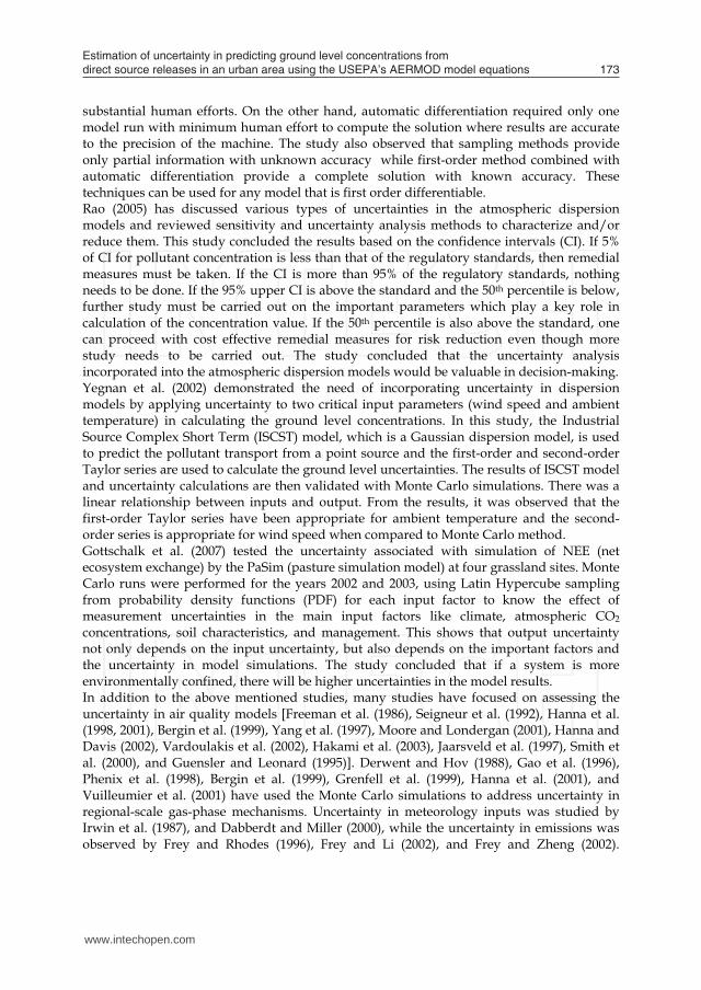
3.1.1a 100 m Stack The predicted concentrations from 100 m high stacks for the defined assumption cells have shown an uncertainty range of 55 to 80% for an error of ± 10% (i.e., uncertainty of the concentration equations to calculate ground level concentration within a range of 10% from the predicted value) for all the parameters in convective boundary layer (CBL) for surface roughness length (Zo) value of 0.03 meter. When Zo is 1 meter, the uncertainty ranged between 72 and 74%. In the case of stable boundary layer, the uncertainty ranged from 40 to 45% for the defined assumption cells. Bhat (2008) performed uncertainty and sensitivity analyses for two Gaussian models used by Bower et al. (1979) and Chen et al. (1998) for modeling bioaerosol emissions from land applications of class B biosolids. He observed uncertainty ranges of 54 to 63% and 55 to 60% for Bowers et al. (1979) and Chen et al. (1998) models respectively, for a ground level source. Figures 1 through 6 present the uncertainty charts for both convective and stable atmospheric conditions at different downwind distances. It was observed that the atmospheric stability conditions influenced the uncertainty value. The uncertainty value decreased as the atmospheric stability condition changed from convective to stable.

www.intechopen.com

Estimation of uncertainty in predicting ground level concentrations from direct source releases in an urban area using the USEPA’s AERMOD model equations 183

forecasting cell, and parameters such as emission rate, stack exit velocity, stack temperature, wind speed, lateral dispersion parameter, vertical dispersion parameter, weighting coefficients for both updraft and downdraft, total horizontal distribution function, cloud cover, ambient temperature, and surface roughness length are defined as assumption cells. Their corresponding probability distribution functions, depending on the measured or practical values are assigned to get the uncertainty and sensitivity analyses of the forecasting cell in both convective and stable conditions (refer to Table 6). In addition to the above input values, convective mixing height is also taken as another assumption cell in CBL as the value of convective mixing height is directly taken, rather than calculating it using its integral form of equation. Convective mixing height governs the equation of total vertical turbulence, which is used for calculating the vertical dispersion parameter. An accepted error of ±10% of the value is applied for the parameters in both assumption and forecasting cells while performing uncertainty and sensitivity analyses in predicting ground level concentrations. For each set of data, the analyses are carried at different downwind distances. In the case of height of stacks being constant, uncertainty and sensitivity analyses were performed at three different downwind distances: distance near the maximum concentration value, next nearest distance point to the stack coordinates, and a farthest point. For the other cases where the range for parameters wind speed, Monin-Obukhov length, and ambient temperature are considered, the hour with the lowest and highest value from range are taken (refer to Table 7) and the predicted concentrations from that hour are considered for uncertainty and sensitivity analysis. These values are applicable for the days considered. For CBL condition, separate case is considered by taking two values of surface roughness length (0.03 m for urban area with isolated obstructions and 1 m for urban area with large buildings).

Parameter

Probability Distribution Function

Reference CBL SBL

Lateral distribution (σy) Gaussian Gaussian Willis and Deardorff (1981), Briggs (1993)

Vertical distribution (σz) bi-Gaussian Gaussian Willis and Deardorff (1981), Briggs (1993)

Wind velocity (u) Weibull Weibull Sathyajith (2002)

Total horizontal distribution function (Fy) Gaussian Gaussian Lamb (1982)

Weighting coefficients for both updraft and downdraft (λ1 and λ2)

bi-Gaussian NA Weil et al. (1997)

Stack exit temperature (T) Gaussian Gaussian Gabriel (1994)

Stack exit velocity (Ws) Gaussian Gaussian

Emission rate (Q) Gaussian Gaussian Eugene et al. (2008) Table 6. Assumption Cells and Their Assigned Probability Distribution Functions.

Parameter

SBL CBL

Lowest Highest Lowest Highest

Wind speed (ms-1) 1.5 9.3 3.6 8.2

Ambient temperature (oK) 262.5 294.9 267.5 302

Monin-Obukhov length (m) 38.4 8888 -8888 -356

Table 7. Summary of Parameters Considered for Uncertainty and Sensitivity Analyses.

3. Results and discussion 3.1 Uncertainty Analysis

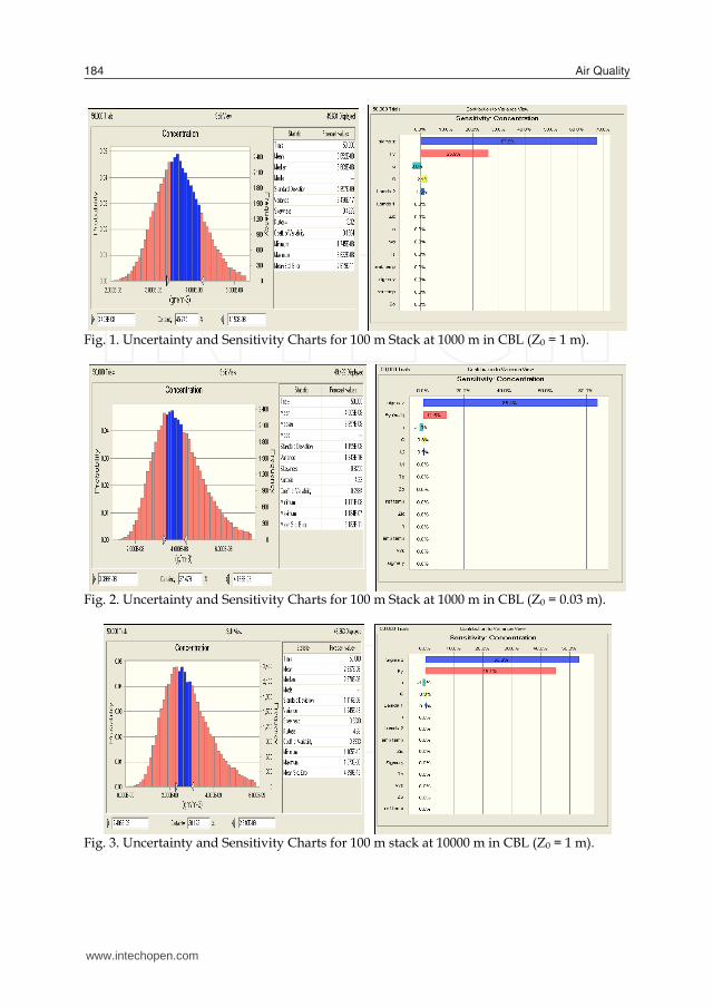
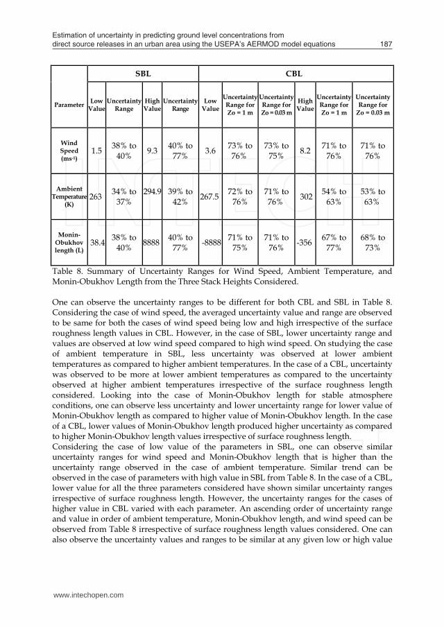
3.1.1a 100 m Stack The predicted concentrations from 100 m high stacks for the defined assumption cells have shown an uncertainty range of 55 to 80% for an error of ± 10% (i.e., uncertainty of the concentration equations to calculate ground level concentration within a range of 10% from the predicted value) for all the parameters in convective boundary layer (CBL) for surface roughness length (Zo) value of 0.03 meter. When Zo is 1 meter, the uncertainty ranged between 72 and 74%. In the case of stable boundary layer, the uncertainty ranged from 40 to 45% for the defined assumption cells. Bhat (2008) performed uncertainty and sensitivity analyses for two Gaussian models used by Bower et al. (1979) and Chen et al. (1998) for modeling bioaerosol emissions from land applications of class B biosolids. He observed uncertainty ranges of 54 to 63% and 55 to 60% for Bowers et al. (1979) and Chen et al. (1998) models respectively, for a ground level source. Figures 1 through 6 present the uncertainty charts for both convective and stable atmospheric conditions at different downwind distances. It was observed that the atmospheric stability conditions influenced the uncertainty value. The uncertainty value decreased as the atmospheric stability condition changed from convective to stable.

www.intechopen.com

Air Quality184

Fig. 1. Uncertainty and Sensitivity Charts for 100 m Stack at 1000 m in CBL (Z0 = 1 m).

Fig. 2. Uncertainty and Sensitivity Charts for 100 m Stack at 1000 m in CBL (Z0 = 0.03 m).

Fig. 3. Uncertainty and Sensitivity Charts for 100 m stack at 10000 m in CBL (Z0 = 1 m).

Fig. 4. Uncertainty and Sensitivity Charts for 100 m stack at 10000 m in CBL (Z0 = 0.03 m).

Fig. 5. Uncertainty and Sensitivity Charts for 100 m stack at 1000 m in SBL.

Fig. 6. Uncertainty and Sensitivity Charts for 100 m stack at 10000 m in SBL.

www.intechopen.com

Estimation of uncertainty in predicting ground level concentrations from direct source releases in an urban area using the USEPA’s AERMOD model equations 185

Fig. 1. Uncertainty and Sensitivity Charts for 100 m Stack at 1000 m in CBL (Z0 = 1 m).

Fig. 2. Uncertainty and Sensitivity Charts for 100 m Stack at 1000 m in CBL (Z0 = 0.03 m).

Fig. 3. Uncertainty and Sensitivity Charts for 100 m stack at 10000 m in CBL (Z0 = 1 m).

Fig. 4. Uncertainty and Sensitivity Charts for 100 m stack at 10000 m in CBL (Z0 = 0.03 m).

Fig. 5. Uncertainty and Sensitivity Charts for 100 m stack at 1000 m in SBL.

Fig. 6. Uncertainty and Sensitivity Charts for 100 m stack at 10000 m in SBL.

www.intechopen.com

Air Quality186

The uncertainty analysis was also carried out for a 70 m and 40 m stack and the results obtained are summarized below.

3.1.1b 70 m Stack The predicted concentrations from a 70 m stack for the defined assumption cells have shown an uncertainty range of 72 to 77% for an error of ± 10% for all the parameters in CBL for Zo = 0.03 m, and for the cases where Zo = 1 m, the uncertainty varied between 72 and 76%.i.e. there is only 23 to 28% certainty that the predicted concentration will lie within the range of 10% from the actual concentration. In the case of SBL, an uncertainty range of 41 to 48% was observed for the defined assumption cells concluding that the certainty of predicting concentration is almost 52 to 59%.

3.1.1c 40 m Stack The predicted concentrations from the 40 m stack for the defined assumption cells have shown an uncertainty range of 70 to 77% and 70 to 76% for an error of ± 10% for all the parameters in CBL for Zo = 0.03 m and Zo = 1 m respectively. In other words, the prediction of concentration for 40 m stack is 27 to 30% times within the 10% range from observed concentration. In the case of SBL, an uncertainty range of 41 to 47% was observed for the defined assumptions cells. From the above results it is clear that the prediction of concentration is less uncertain in stable case as compared to the convective cases. The spreadsheet predict shows more certainty in predicting concentrations in SBL as compared to that in CBL. Uncertainty ranges for SBL and the case of CBL representing an urban area with large buildings were found to be similar irrespective of the stack height considered. However, the uncertainty ranges varied for the case of CBL representing an urban area with isolated buildings. The influence of surface roughness is found to be more pronounced for a tall stack of 100 m where a much wider range of uncertainty was observed as compared to 40 m and 70 m stack height cases. The uncertainty in concentration results is not influenced by surface roughness for 70 m and 40 m stacks.

3.1.2 Uncertainty Analysis Summary Table 8 provides a summary of the uncertainty ranges observed from the uncertainty charts for the cases with the lowest and highest value of the parameters from the range of values for the three days taken for analysis.

SBL CBL

Parameter Low Value

Uncertainty Range

High Value

Uncertainty Range

Low Value

Uncertainty Range for Zo = 1 m

Uncertainty Range for Zo = 0.03 m

High Value

Uncertainty Range for Zo = 1 m

Uncertainty Range for

Zo = 0.03 m

Wind Speed (ms-1)

1.5 38% to 40% 9.3 40% to

77% 3.6 73% to 76%

73% to 75% 8.2 71% to

76% 71% to

76%

Ambient Temperature

(K) 263 34% to

37% 294.9

39% to

42% 267.5 72% to 76%

71% to 76% 302 54% to

63% 53% to 63%

Monin-Obukhov length (L)

38.4 38% to 40% 8888 40% to

77% -8888 71% to 75%

71% to 76% -356 67% to

77% 68% to

73%

Table 8. Summary of Uncertainty Ranges for Wind Speed, Ambient Temperature, and Monin-Obukhov Length from the Three Stack Heights Considered. One can observe the uncertainty ranges to be different for both CBL and SBL in Table 8. Considering the case of wind speed, the averaged uncertainty value and range are observed to be same for both the cases of wind speed being low and high irrespective of the surface roughness length values in CBL. However, in the case of SBL, lower uncertainty range and values are observed at low wind speed compared to high wind speed. On studying the case of ambient temperature in SBL, less uncertainty was observed at lower ambient temperatures as compared to higher ambient temperatures. In the case of a CBL, uncertainty was observed to be more at lower ambient temperatures as compared to the uncertainty observed at higher ambient temperatures irrespective of the surface roughness length considered. Looking into the case of Monin-Obukhov length for stable atmosphere conditions, one can observe less uncertainty and lower uncertainty range for lower value of Monin-Obukhov length as compared to higher value of Monin-Obukhov length. In the case of a CBL, lower values of Monin-Obukhov length produced higher uncertainty as compared to higher Monin-Obukhov length values irrespective of surface roughness length. Considering the case of low value of the parameters in SBL, one can observe similar uncertainty ranges for wind speed and Monin-Obukhov length that is higher than the uncertainty range observed in the case of ambient temperature. Similar trend can be observed in the case of parameters with high value in SBL from Table 8. In the case of a CBL, lower value for all the three parameters considered have shown similar uncertainty ranges irrespective of surface roughness length. However, the uncertainty ranges for the cases of higher value in CBL varied with each parameter. An ascending order of uncertainty range and value in order of ambient temperature, Monin-Obukhov length, and wind speed can be observed from Table 8 irrespective of surface roughness length values considered. One can also observe the uncertainty values and ranges to be similar at any given low or high value

www.intechopen.com

Estimation of uncertainty in predicting ground level concentrations from direct source releases in an urban area using the USEPA’s AERMOD model equations 187

The uncertainty analysis was also carried out for a 70 m and 40 m stack and the results obtained are summarized below.

3.1.1b 70 m Stack The predicted concentrations from a 70 m stack for the defined assumption cells have shown an uncertainty range of 72 to 77% for an error of ± 10% for all the parameters in CBL for Zo = 0.03 m, and for the cases where Zo = 1 m, the uncertainty varied between 72 and 76%.i.e. there is only 23 to 28% certainty that the predicted concentration will lie within the range of 10% from the actual concentration. In the case of SBL, an uncertainty range of 41 to 48% was observed for the defined assumption cells concluding that the certainty of predicting concentration is almost 52 to 59%.

3.1.1c 40 m Stack The predicted concentrations from the 40 m stack for the defined assumption cells have shown an uncertainty range of 70 to 77% and 70 to 76% for an error of ± 10% for all the parameters in CBL for Zo = 0.03 m and Zo = 1 m respectively. In other words, the prediction of concentration for 40 m stack is 27 to 30% times within the 10% range from observed concentration. In the case of SBL, an uncertainty range of 41 to 47% was observed for the defined assumptions cells. From the above results it is clear that the prediction of concentration is less uncertain in stable case as compared to the convective cases. The spreadsheet predict shows more certainty in predicting concentrations in SBL as compared to that in CBL. Uncertainty ranges for SBL and the case of CBL representing an urban area with large buildings were found to be similar irrespective of the stack height considered. However, the uncertainty ranges varied for the case of CBL representing an urban area with isolated buildings. The influence of surface roughness is found to be more pronounced for a tall stack of 100 m where a much wider range of uncertainty was observed as compared to 40 m and 70 m stack height cases. The uncertainty in concentration results is not influenced by surface roughness for 70 m and 40 m stacks.

3.1.2 Uncertainty Analysis Summary Table 8 provides a summary of the uncertainty ranges observed from the uncertainty charts for the cases with the lowest and highest value of the parameters from the range of values for the three days taken for analysis.

SBL CBL

Parameter Low Value

Uncertainty Range

High Value

Uncertainty Range

Low Value

Uncertainty Range for Zo = 1 m

Uncertainty Range for Zo = 0.03 m

High Value

Uncertainty Range for Zo = 1 m

Uncertainty Range for

Zo = 0.03 m

Wind Speed (ms-1)

1.5 38% to 40% 9.3 40% to

77% 3.6 73% to 76%

73% to 75% 8.2 71% to

76% 71% to

76%

Ambient Temperature

(K) 263 34% to

37% 294.9

39% to

42% 267.5 72% to 76%

71% to 76% 302 54% to

63% 53% to 63%

Monin-Obukhov length (L)

38.4 38% to 40% 8888 40% to

77% -8888 71% to 75%

71% to 76% -356 67% to

77% 68% to

73%

Table 8. Summary of Uncertainty Ranges for Wind Speed, Ambient Temperature, and Monin-Obukhov Length from the Three Stack Heights Considered. One can observe the uncertainty ranges to be different for both CBL and SBL in Table 8. Considering the case of wind speed, the averaged uncertainty value and range are observed to be same for both the cases of wind speed being low and high irrespective of the surface roughness length values in CBL. However, in the case of SBL, lower uncertainty range and values are observed at low wind speed compared to high wind speed. On studying the case of ambient temperature in SBL, less uncertainty was observed at lower ambient temperatures as compared to higher ambient temperatures. In the case of a CBL, uncertainty was observed to be more at lower ambient temperatures as compared to the uncertainty observed at higher ambient temperatures irrespective of the surface roughness length considered. Looking into the case of Monin-Obukhov length for stable atmosphere conditions, one can observe less uncertainty and lower uncertainty range for lower value of Monin-Obukhov length as compared to higher value of Monin-Obukhov length. In the case of a CBL, lower values of Monin-Obukhov length produced higher uncertainty as compared to higher Monin-Obukhov length values irrespective of surface roughness length. Considering the case of low value of the parameters in SBL, one can observe similar uncertainty ranges for wind speed and Monin-Obukhov length that is higher than the uncertainty range observed in the case of ambient temperature. Similar trend can be observed in the case of parameters with high value in SBL from Table 8. In the case of a CBL, lower value for all the three parameters considered have shown similar uncertainty ranges irrespective of surface roughness length. However, the uncertainty ranges for the cases of higher value in CBL varied with each parameter. An ascending order of uncertainty range and value in order of ambient temperature, Monin-Obukhov length, and wind speed can be observed from Table 8 irrespective of surface roughness length values considered. One can also observe the uncertainty values and ranges to be similar at any given low or high value

www.intechopen.com

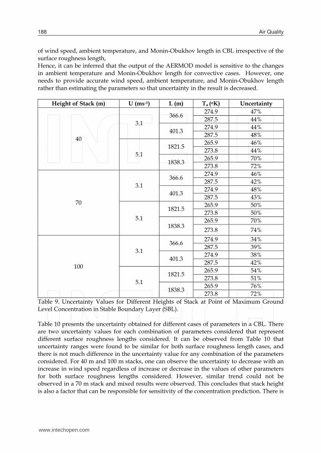
Air Quality188

of wind speed, ambient temperature, and Monin-Obukhov length in CBL irrespective of the surface roughness length, Hence, it can be inferred that the output of the AERMOD model is sensitive to the changes in ambient temperature and Monin-Obukhov length for convective cases. However, one needs to provide accurate wind speed, ambient temperature, and Monin-Obukhov length rather than estimating the parameters so that uncertainty in the result is decreased.

Height of Stack (m) U (ms-1) L (m) Ta (oK) Uncertainty

40

3.1 366.6 274.9 47%

287.5 44%

401.3 274.9 44% 287.5 48%

5.1 1821.5 265.9 46%

273.8 44%

1838.3 265.9 70% 273.8 72%

70

3.1 366.6 274.9 46%

287.5 42%

401.3 274.9 48% 287.5 43%

5.1 1821.5 265.9 50%

273.8 50%

1838.3 265.9 70% 273.8 74%

100

3.1 366.6 274.9 34%

287.5 39%

401.3 274.9 38% 287.5 42%

5.1 1821.5 265.9 54%

273.8 51%

1838.3 265.9 76% 273.8 72%

Table 9. Uncertainty Values for Different Heights of Stack at Point of Maximum Ground Level Concentration in Stable Boundary Layer (SBL). Table 10 presents the uncertainty obtained for different cases of parameters in a CBL. There are two uncertainty values for each combination of parameters considered that represent different surface roughness lengths considered. It can be observed from Table 10 that uncertainty ranges were found to be similar for both surface roughness length cases, and there is not much difference in the uncertainty value for any combination of the parameters considered. For 40 m and 100 m stacks, one can observe the uncertainty to decrease with an increase in wind speed regardless of increase or decrease in the values of other parameters for both surface roughness lengths considered. However, similar trend could not be observed in a 70 m stack and mixed results were observed. This concludes that stack height is also a factor that can be responsible for sensitivity of the concentration prediction. There is

need to calculate the uncertainty in calculations due to stack height variation. It can also be seen from Table 10 that irrespective of the ambient temperature, uncertainty observed for a combination of lower values of wind speed and Monin-Obukhov length is more compared to uncertainty observed for a combination of higher values of wind speed and Monin-Obukhov length. Hence, one can infer the uncertainty to be more at lower parameter values than higher parameter values for CBL conditions.

Height of stack (m) U (ms-1) L (m) Ta (oK) Uncertainty

Zo = 0.03 m Zo = 1 m

40

4.1 -2423.7 267.5 73% 70%

295.9 73% 75%

-356 267.5 75% 72% 295.9 73% 68%

6.7 -3345.8 268.1 68% 68%

302 65% 60%

-957.2 268.1 58% 63% 302 54% 53%

70

4.1 -2423.7 267.5 73% 73%

295.9 70% 68%

-356 267.5 70% 68% 295.9 70% 69%

6.7 -3345.8 268.1 75% 72%

302 68% 63%

-957.2 268.1 72% 76% 302 63% 75%

100

4.1 -2423.7 267.5 76% 70%

295.9 75% 74%

-356 267.5 63% 62% 295.9 54% 59%

6.7 -3345.8 268.1 68% 70%

302 60% 70%

-957.2 268.1 63% 58% 302 53% 54%

Table 10. Uncertainty Values for Different Heights of Stack at Point of Maximum Ground Level Concentration in Convective Boundary Layer (CBL). Irrespective of the stack heights considered, one can infer the uncertainty to be more at higher wind speed, Monin-Obukhov length, and ambient temperature for stable boundary conditions. An opposite trend is observed for CBL conditions, i.e., uncertainty was observed to be more at lower wind speed, Monin-Obukhov length, and ambient temperature. One can observe

www.intechopen.com

Estimation of uncertainty in predicting ground level concentrations from direct source releases in an urban area using the USEPA’s AERMOD model equations 189

of wind speed, ambient temperature, and Monin-Obukhov length in CBL irrespective of the surface roughness length, Hence, it can be inferred that the output of the AERMOD model is sensitive to the changes in ambient temperature and Monin-Obukhov length for convective cases. However, one needs to provide accurate wind speed, ambient temperature, and Monin-Obukhov length rather than estimating the parameters so that uncertainty in the result is decreased.

Height of Stack (m) U (ms-1) L (m) Ta (oK) Uncertainty

40

3.1 366.6 274.9 47%

287.5 44%

401.3 274.9 44% 287.5 48%

5.1 1821.5 265.9 46%

273.8 44%

1838.3 265.9 70% 273.8 72%

70

3.1 366.6 274.9 46%

287.5 42%

401.3 274.9 48% 287.5 43%

5.1 1821.5 265.9 50%

273.8 50%

1838.3 265.9 70% 273.8 74%

100

3.1 366.6 274.9 34%

287.5 39%

401.3 274.9 38% 287.5 42%

5.1 1821.5 265.9 54%

273.8 51%

1838.3 265.9 76% 273.8 72%

Table 9. Uncertainty Values for Different Heights of Stack at Point of Maximum Ground Level Concentration in Stable Boundary Layer (SBL). Table 10 presents the uncertainty obtained for different cases of parameters in a CBL. There are two uncertainty values for each combination of parameters considered that represent different surface roughness lengths considered. It can be observed from Table 10 that uncertainty ranges were found to be similar for both surface roughness length cases, and there is not much difference in the uncertainty value for any combination of the parameters considered. For 40 m and 100 m stacks, one can observe the uncertainty to decrease with an increase in wind speed regardless of increase or decrease in the values of other parameters for both surface roughness lengths considered. However, similar trend could not be observed in a 70 m stack and mixed results were observed. This concludes that stack height is also a factor that can be responsible for sensitivity of the concentration prediction. There is

need to calculate the uncertainty in calculations due to stack height variation. It can also be seen from Table 10 that irrespective of the ambient temperature, uncertainty observed for a combination of lower values of wind speed and Monin-Obukhov length is more compared to uncertainty observed for a combination of higher values of wind speed and Monin-Obukhov length. Hence, one can infer the uncertainty to be more at lower parameter values than higher parameter values for CBL conditions.

Height of stack (m) U (ms-1) L (m) Ta (oK) Uncertainty

Zo = 0.03 m Zo = 1 m

40

4.1 -2423.7 267.5 73% 70%

295.9 73% 75%

-356 267.5 75% 72% 295.9 73% 68%

6.7 -3345.8 268.1 68% 68%

302 65% 60%

-957.2 268.1 58% 63% 302 54% 53%

70

4.1 -2423.7 267.5 73% 73%

295.9 70% 68%

-356 267.5 70% 68% 295.9 70% 69%

6.7 -3345.8 268.1 75% 72%

302 68% 63%

-957.2 268.1 72% 76% 302 63% 75%

100

4.1 -2423.7 267.5 76% 70%

295.9 75% 74%

-356 267.5 63% 62% 295.9 54% 59%

6.7 -3345.8 268.1 68% 70%

302 60% 70%

-957.2 268.1 63% 58% 302 53% 54%

Table 10. Uncertainty Values for Different Heights of Stack at Point of Maximum Ground Level Concentration in Convective Boundary Layer (CBL). Irrespective of the stack heights considered, one can infer the uncertainty to be more at higher wind speed, Monin-Obukhov length, and ambient temperature for stable boundary conditions. An opposite trend is observed for CBL conditions, i.e., uncertainty was observed to be more at lower wind speed, Monin-Obukhov length, and ambient temperature. One can observe

www.intechopen.com

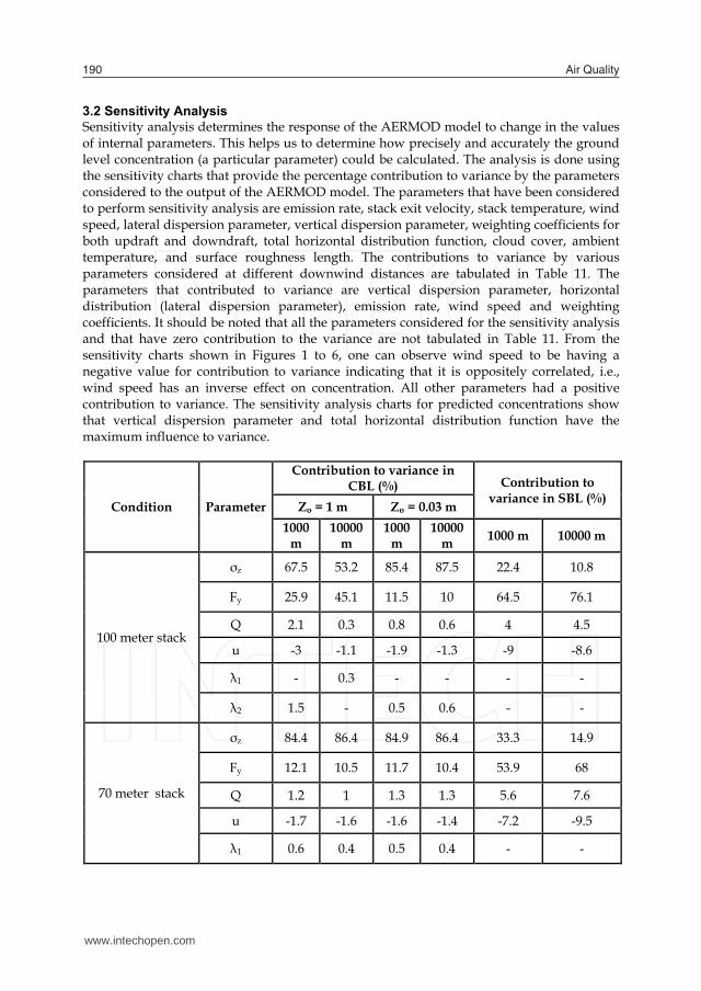
Air Quality190

3.2 Sensitivity Analysis Sensitivity analysis determines the response of the AERMOD model to change in the values of internal parameters. This helps us to determine how precisely and accurately the ground level concentration (a particular parameter) could be calculated. The analysis is done using the sensitivity charts that provide the percentage contribution to variance by the parameters considered to the output of the AERMOD model. The parameters that have been considered to perform sensitivity analysis are emission rate, stack exit velocity, stack temperature, wind speed, lateral dispersion parameter, vertical dispersion parameter, weighting coefficients for both updraft and downdraft, total horizontal distribution function, cloud cover, ambient temperature, and surface roughness length. The contributions to variance by various parameters considered at different downwind distances are tabulated in Table 11. The parameters that contributed to variance are vertical dispersion parameter, horizontal distribution (lateral dispersion parameter), emission rate, wind speed and weighting coefficients. It should be noted that all the parameters considered for the sensitivity analysis and that have zero contribution to the variance are not tabulated in Table 11. From the sensitivity charts shown in Figures 1 to 6, one can observe wind speed to be having a negative value for contribution to variance indicating that it is oppositely correlated, i.e., wind speed has an inverse effect on concentration. All other parameters had a positive contribution to variance. The sensitivity analysis charts for predicted concentrations show that vertical dispersion parameter and total horizontal distribution function have the maximum influence to variance.

Condition Parameter

Contribution to variance in CBL (%) Contribution to

variance in SBL (%) Zo = 1 m Zo = 0.03 m 1000

m 10000

m 1000

m 10000

m 1000 m 10000 m

100 meter stack

σz 67.5 53.2 85.4 87.5 22.4 10.8

Fy 25.9 45.1 11.5 10 64.5 76.1

Q 2.1 0.3 0.8 0.6 4 4.5

u -3 -1.1 -1.9 -1.3 -9 -8.6

λ1 - 0.3 - - - -

λ2 1.5 - 0.5 0.6 - -

70 meter stack

σz 84.4 86.4 84.9 86.4 33.3 14.9

Fy 12.1 10.5 11.7 10.4 53.9 68

Q 1.2 1 1.3 1.3 5.6 7.6

u -1.7 -1.6 -1.6 -1.4 -7.2 -9.5

λ1 0.6 0.4 0.5 0.4 - -

40 meter stack

σz 82.1 85.9 81.9 85.7 28.4 15.9

Fy 13.6 11.1 14.1 11.1 58.2 66.2

Q 1.6 1.1 1.6 1.2 6.3 6.7

u -2.1 -1.4 -2 -1.6 -7.1 -11.2

λ1 - 0.5 - 0.5 - -

λ2 0.6 - 0.4 - - -

Low wind speed

σz 85.9 89.2 86 89.2 0 0.1

Fy 11.7 8.7 11.4 9.1 84.1 83.9

Q 0.7 0.4 0.8 0.5 4.6 5.1

u -1.1 -1.4 -1.3 -0.8 -11.3 -10.8

λ1 0.5 0.3 0.5 0.3 - -

High wind speed

σz 84.3 89.4 83.3 89.4 5.2 4.7

Fy 13.8 8.7 13.4 8.4 78.8 79.7

Q 1 0.5 0.8 0.6 1.2 4.7

u -0.4 -1.1 -2 -1.2 -2.5 -10.8

λ1 0.4 0.3 0.5 0.3 - -

Low ambient temperature

σz 84.3 88.8 84.2 88.9 0.1 1.2

Fy 12.4 8.9 12.6 8.9 84.2 82.9

Q 0.8 0.6 0.8 0.7 5 4.9

u -1.9 -1.3 -1.9 -1.2 -10.7 -11

λ1 0.6 0.3 0.5 0.4 - -

High ambient temperature

σz 49.2 70.9 49.5 71.5 34.4 1.2

Fy 41.6 23.5 40.4 23.2 55.7 83.1

Q 2.3 1.4 2.7 1.5 3.2 4.9

u -5.5 -3.3 -5.7 -3 -6.6 -10.9

λ1 1.5 0.9 1.6 0.9 - -

www.intechopen.com

Estimation of uncertainty in predicting ground level concentrations from direct source releases in an urban area using the USEPA’s AERMOD model equations 191

3.2 Sensitivity Analysis Sensitivity analysis determines the response of the AERMOD model to change in the values of internal parameters. This helps us to determine how precisely and accurately the ground level concentration (a particular parameter) could be calculated. The analysis is done using the sensitivity charts that provide the percentage contribution to variance by the parameters considered to the output of the AERMOD model. The parameters that have been considered to perform sensitivity analysis are emission rate, stack exit velocity, stack temperature, wind speed, lateral dispersion parameter, vertical dispersion parameter, weighting coefficients for both updraft and downdraft, total horizontal distribution function, cloud cover, ambient temperature, and surface roughness length. The contributions to variance by various parameters considered at different downwind distances are tabulated in Table 11. The parameters that contributed to variance are vertical dispersion parameter, horizontal distribution (lateral dispersion parameter), emission rate, wind speed and weighting coefficients. It should be noted that all the parameters considered for the sensitivity analysis and that have zero contribution to the variance are not tabulated in Table 11. From the sensitivity charts shown in Figures 1 to 6, one can observe wind speed to be having a negative value for contribution to variance indicating that it is oppositely correlated, i.e., wind speed has an inverse effect on concentration. All other parameters had a positive contribution to variance. The sensitivity analysis charts for predicted concentrations show that vertical dispersion parameter and total horizontal distribution function have the maximum influence to variance.

Condition Parameter

Contribution to variance in CBL (%) Contribution to

variance in SBL (%) Zo = 1 m Zo = 0.03 m 1000

m 10000

m 1000

m 10000

m 1000 m 10000 m

100 meter stack

σz 67.5 53.2 85.4 87.5 22.4 10.8

Fy 25.9 45.1 11.5 10 64.5 76.1

Q 2.1 0.3 0.8 0.6 4 4.5

u -3 -1.1 -1.9 -1.3 -9 -8.6

λ1 - 0.3 - - - -

λ2 1.5 - 0.5 0.6 - -

70 meter stack

σz 84.4 86.4 84.9 86.4 33.3 14.9

Fy 12.1 10.5 11.7 10.4 53.9 68

Q 1.2 1 1.3 1.3 5.6 7.6

u -1.7 -1.6 -1.6 -1.4 -7.2 -9.5

λ1 0.6 0.4 0.5 0.4 - -

40 meter stack

σz 82.1 85.9 81.9 85.7 28.4 15.9

Fy 13.6 11.1 14.1 11.1 58.2 66.2

Q 1.6 1.1 1.6 1.2 6.3 6.7

u -2.1 -1.4 -2 -1.6 -7.1 -11.2

λ1 - 0.5 - 0.5 - -

λ2 0.6 - 0.4 - - -

Low wind speed

σz 85.9 89.2 86 89.2 0 0.1

Fy 11.7 8.7 11.4 9.1 84.1 83.9

Q 0.7 0.4 0.8 0.5 4.6 5.1

u -1.1 -1.4 -1.3 -0.8 -11.3 -10.8

λ1 0.5 0.3 0.5 0.3 - -

High wind speed

σz 84.3 89.4 83.3 89.4 5.2 4.7

Fy 13.8 8.7 13.4 8.4 78.8 79.7

Q 1 0.5 0.8 0.6 1.2 4.7

u -0.4 -1.1 -2 -1.2 -2.5 -10.8

λ1 0.4 0.3 0.5 0.3 - -

Low ambient temperature

σz 84.3 88.8 84.2 88.9 0.1 1.2

Fy 12.4 8.9 12.6 8.9 84.2 82.9

Q 0.8 0.6 0.8 0.7 5 4.9

u -1.9 -1.3 -1.9 -1.2 -10.7 -11

λ1 0.6 0.3 0.5 0.4 - -

High ambient temperature

σz 49.2 70.9 49.5 71.5 34.4 1.2

Fy 41.6 23.5 40.4 23.2 55.7 83.1

Q 2.3 1.4 2.7 1.5 3.2 4.9

u -5.5 -3.3 -5.7 -3 -6.6 -10.9

λ1 1.5 0.9 1.6 0.9 - -

www.intechopen.com

Air Quality192

Low Monin- Obukhov length

σz 83.7 89.1 83.6 89.0 0 0.1

Fy 13.1 8.9 13.2 8.7 84.1 83.9

Q 0.9 0.4 0.9 0.5 4.6 5.1

u -1.7 -1.2 -1.8 -1.3 -11.3 -10.8

λ1 0.5 0.4 0.5 0.4 - -

High Monin- Obukhov length

σz 76.9 84.3 77.5 87.5 5.2 4.7

Fy 18.8 9.4 18.1 9.7 78.8 79.7

Q 1 0.6 1.0 0.7 1.2 4.7

U -2.7 -5.3 -2.6 -1.5 -2.5 -10.8

λ1 0.6 0.4 0.8 0.5 - -

Table 11. Contribution to Variance by Parameters in Calculation of Concentration at Different Downwind Distances. The contributions to variance of parameters in both CBL and SBL for 1000 m and 10000 m downwind distance are tabulated in Table 11. In CBL, contribution to variance by vertical dispersion parameter is more than the contribution from horizontal distribution function which is a function of lateral dispersion parameter, indicating pollutant concentration to be more sensitive to vertical dispersion parameter than lateral dispersion parameter. However, it is the opposite in SBL, i.e., pollutant concentration is more sensitive to lateral dispersion parameter than vertical dispersion parameter. Wind speed parameter had a negative contribution to variance irrespective of the boundary layer conditions at both downwind distances. The contribution to variance by weighting coefficients is found to be negligible in all the conditions. For the condition considering stack heights from Table 11, the pollutant concentration sensitiveness increased with downwind distance for vertical dispersion parameter and wind speed, but decreased for the remaining parameters in CBL for both surface roughness lengths considered. In SBL, contribution to variance by vertical dispersion parameter reduced with increase in downwind distance and increased for all other parameters considered for analysis. For the condition considering low and high wind speeds from Table 11, in CBL, the pollutant concentration sensitiveness increased with downwind distance for vertical dispersion parameter. Pollutant concentration sensitiveness varied with surface roughness. For the case of Z0 being 1 m pollutant concentration sensitiveness decreased with increase in downwind distance and the opposite trend is observed for the case of Z0 being 0.03 m. For all other parameters pollutant concentration sensitiveness decreased with increase in downwind distance. In SBL, pollutant concentration sensitiveness decreased for vertical dispersion parameter as downwind distance increased and one can note that for lower wind speed, the contribution to variance by vertical dispersion parameter is zero at both 1000 m and 10000 m.

For the condition of ambient temperature in CBL, the contribution of variance by vertical dispersion parameter and wind speed increased with downwind distance and decreased for all other parameters for both the surface roughness lengths considered. Similar pattern can be observed in SBL for the condition of lower ambient temperature with the exception that wind speed showed an opposite trend to that observed in CBL. However, for the case of higher ambient temperature, in SBL, the contribution to variance increases for horizontal distribution and emission rate, and decreases for vertical dispersion parameter and wind speed with increase in downwind distance. For both high and low values of ambient temperature, the contribution by wind speed was significant in SBL compared to CBL. Thus, one can state that the concentrations are more sensitive to higher temperatures and wind speed in SBL than in CBL. The sensitiveness in Monin-Obukhov length condition showed similar behavior to that of wind speed condition. It was observed that emission rate had more contribution to variance than vertical dispersion parameter in SBL for the cases having lower values of Monin-Obukhov length, wind speed, and ambient temperature. The remaining parameters defined in the assumption cells have negligible contribution to variance when compared to vertical dispersion parameter and total horizontal distribution function.

4. Conclusions The objective of the study was to perform uncertainty and sensitivity analyses in predicting the concentrations from the AERMOD equations. As it is difficult to perform uncertainty and sensitivity analyses using the original AERMOD model, an approximate set of AERMOD equations were programmed in Excel. The predicted concentrations from the AERMODCBL and AERMODSBL models were compared to the predicted concentrations from AERMOD model. The comparison has shown that the predicted concentration values from the spreadsheet ranged between 87% and 107%, as compared to the predicted concentration values from the AERMOD model. This showed that the predicted concentrations obtained by the modeled equations can be relied upon to perform uncertainty and sensitivity analyses for both atmospheric conditions. Uncertainty and sensitivity analysis has been performed for different cases taken into consideration by varying stack height, wind speed, Monin-Obukhov length, and ambient temperature for three days and source data as summarized in Tables 3, 4, and 5. The conclusions made from the study are listed below.

1. A user-friendly tool [60], that can calculate downwind contaminant concentrations under different boundary layer conditions has been developed using the AERMOD equations.

2. The uncertainty range varies between 67% and 75% for convective conditions on averaging the uncertainty values from all the considered cases, while in stable conditions, it ranged from 40% to 47%. This means the predictions are less certain in convective cases.

3. The contribution to variance by vertical dispersion parameter (σz) is found to be 82% under convective conditions i.e. the predicted concentrations are highly influenced by σz.. In the case of horizontal distribution (Fy), the contribution to variance was found to be 75% in the stable case.

www.intechopen.com

Estimation of uncertainty in predicting ground level concentrations from direct source releases in an urban area using the USEPA’s AERMOD model equations 193

Low Monin- Obukhov length

σz 83.7 89.1 83.6 89.0 0 0.1

Fy 13.1 8.9 13.2 8.7 84.1 83.9

Q 0.9 0.4 0.9 0.5 4.6 5.1

u -1.7 -1.2 -1.8 -1.3 -11.3 -10.8

λ1 0.5 0.4 0.5 0.4 - -

High Monin- Obukhov length

σz 76.9 84.3 77.5 87.5 5.2 4.7

Fy 18.8 9.4 18.1 9.7 78.8 79.7

Q 1 0.6 1.0 0.7 1.2 4.7

U -2.7 -5.3 -2.6 -1.5 -2.5 -10.8

λ1 0.6 0.4 0.8 0.5 - -

Table 11. Contribution to Variance by Parameters in Calculation of Concentration at Different Downwind Distances. The contributions to variance of parameters in both CBL and SBL for 1000 m and 10000 m downwind distance are tabulated in Table 11. In CBL, contribution to variance by vertical dispersion parameter is more than the contribution from horizontal distribution function which is a function of lateral dispersion parameter, indicating pollutant concentration to be more sensitive to vertical dispersion parameter than lateral dispersion parameter. However, it is the opposite in SBL, i.e., pollutant concentration is more sensitive to lateral dispersion parameter than vertical dispersion parameter. Wind speed parameter had a negative contribution to variance irrespective of the boundary layer conditions at both downwind distances. The contribution to variance by weighting coefficients is found to be negligible in all the conditions. For the condition considering stack heights from Table 11, the pollutant concentration sensitiveness increased with downwind distance for vertical dispersion parameter and wind speed, but decreased for the remaining parameters in CBL for both surface roughness lengths considered. In SBL, contribution to variance by vertical dispersion parameter reduced with increase in downwind distance and increased for all other parameters considered for analysis. For the condition considering low and high wind speeds from Table 11, in CBL, the pollutant concentration sensitiveness increased with downwind distance for vertical dispersion parameter. Pollutant concentration sensitiveness varied with surface roughness. For the case of Z0 being 1 m pollutant concentration sensitiveness decreased with increase in downwind distance and the opposite trend is observed for the case of Z0 being 0.03 m. For all other parameters pollutant concentration sensitiveness decreased with increase in downwind distance. In SBL, pollutant concentration sensitiveness decreased for vertical dispersion parameter as downwind distance increased and one can note that for lower wind speed, the contribution to variance by vertical dispersion parameter is zero at both 1000 m and 10000 m.

For the condition of ambient temperature in CBL, the contribution of variance by vertical dispersion parameter and wind speed increased with downwind distance and decreased for all other parameters for both the surface roughness lengths considered. Similar pattern can be observed in SBL for the condition of lower ambient temperature with the exception that wind speed showed an opposite trend to that observed in CBL. However, for the case of higher ambient temperature, in SBL, the contribution to variance increases for horizontal distribution and emission rate, and decreases for vertical dispersion parameter and wind speed with increase in downwind distance. For both high and low values of ambient temperature, the contribution by wind speed was significant in SBL compared to CBL. Thus, one can state that the concentrations are more sensitive to higher temperatures and wind speed in SBL than in CBL. The sensitiveness in Monin-Obukhov length condition showed similar behavior to that of wind speed condition. It was observed that emission rate had more contribution to variance than vertical dispersion parameter in SBL for the cases having lower values of Monin-Obukhov length, wind speed, and ambient temperature. The remaining parameters defined in the assumption cells have negligible contribution to variance when compared to vertical dispersion parameter and total horizontal distribution function.

4. Conclusions The objective of the study was to perform uncertainty and sensitivity analyses in predicting the concentrations from the AERMOD equations. As it is difficult to perform uncertainty and sensitivity analyses using the original AERMOD model, an approximate set of AERMOD equations were programmed in Excel. The predicted concentrations from the AERMODCBL and AERMODSBL models were compared to the predicted concentrations from AERMOD model. The comparison has shown that the predicted concentration values from the spreadsheet ranged between 87% and 107%, as compared to the predicted concentration values from the AERMOD model. This showed that the predicted concentrations obtained by the modeled equations can be relied upon to perform uncertainty and sensitivity analyses for both atmospheric conditions. Uncertainty and sensitivity analysis has been performed for different cases taken into consideration by varying stack height, wind speed, Monin-Obukhov length, and ambient temperature for three days and source data as summarized in Tables 3, 4, and 5. The conclusions made from the study are listed below.

1. A user-friendly tool [60], that can calculate downwind contaminant concentrations under different boundary layer conditions has been developed using the AERMOD equations.

2. The uncertainty range varies between 67% and 75% for convective conditions on averaging the uncertainty values from all the considered cases, while in stable conditions, it ranged from 40% to 47%. This means the predictions are less certain in convective cases.

3. The contribution to variance by vertical dispersion parameter (σz) is found to be 82% under convective conditions i.e. the predicted concentrations are highly influenced by σz.. In the case of horizontal distribution (Fy), the contribution to variance was found to be 75% in the stable case.

www.intechopen.com

Air Quality194

4. In SBL, for low values of wind speed, Monin-Obukhov length, and ambient temperature, the contribution to variance by emission rate (Q) is considerably more than that of vertical dispersion parameter (σz).

5. In CBL, concentration predictions are sensitive to vertical dispersion (σz) and horizontal distribution (Fy), i.e. σy regardless of stack height and surface roughness.

6. In SBL, concentration predictions are sensitive to horizontal distribution (Fy), i.e. σy and vertical dispersion (σz) regardless of the stack heights.

7. The predicted concentration equation is sensitive to vertical dispersion parameter (σz), horizontal distribution (Fy) (lateral dispersion parameter (σy)), and emission rate. Other parameters have negligible or no influence on sensitivity with the exception of wind speed that has a negative correlation.

5. Acknowledgements The authors would like to thank Lakes Environmental for providing a copy of the software for the use in this research work.

6. References Bartell, S.M.; Breck, J.E.; Gardner, R.H.; Brenkert, A.L. Individual parameter perturbation

and error analysis of fish bioenergetics models. Can. J. Fish. Aquat. Sci. 1986, 43, 160-168.

Bergin, M.S.; Noblet, G.S.; Petrini, K.; Dhieux, J.R.; Milford, J.B.; Harley, R.A. Formal uncertainty analysis of a lagrangian photochemical air pollution model. J. Environ. Sci. Technol. 1999, 33, 1116–1126.

Bhat, A.S. Development and evaluation of a screening type dispersion model for bioaerosols emission from land application of Class B biosolids. Master’s Thesis, The University of Toledo. 2008, 78 pp

Bowers, J.F.; Bjorkland J.R.; Cheney C.S. (1979).Industrial Source Complex (ISC) dispersion model user’s guide. U.S. Environmental Protection Agency Report. EPA 450/4-79-030.

Brenkert, A.L.; Gardner, R.H.; Bartell, S.M.; Hoffman, F.O. In Reliability of Radioactive Transfer Models; Desmet, G.; Ed.; Uncertainties associated with estimates of radium accumulation in lake sediments and biota. Elsevier Applied Science: London, UK, 1988; pp 185-192.

Briggs, G.A. Plume dispersion in the convective boundary layer. Part II: analysis of CONDORS field experiment data. J. Appl Meteorol. 1993, 32, 1388-1425.

Cacuci, D.G. Sensitivity theory for nonlinear systems. Part I and II. J. Math. Phys. 1981, 22, 2794-2812.

Chen Y.; Dwaine B.; Steven H. Development of model of dispersion parameters for odour transmission from agricultural sources. J. Agr. Eng. 1998, 69, 229-238.

Cullen, A.C.; Frey, H.C. (1999). Probabilistic techniques in exposure assessment: a handbook for dealing with variability and uncertainty in risk analysis. New York: Plenum Press.

Dabberdt, W.F.; Miller, E. Uncertainty, ensembles, and air quality dispersion modeling: applications and challenges. J. Atmos. Environ. 2000, 34, 4667–4673.

Dempster, A.P. Upper and lower probabilities induced by a multi-valued mapping. Ann. Math. Statistics. 1967, 38, 325–339.

Derwent, R.; Hov, Ø. Application of sensitivity and uncertainty analysis techniques to a photochemical ozone model. J. Geophys. Res. 1988, 93, 5185–5199.

Downing, D.J.; Gardner, R.H.; Hoffman, F.O. An examination of response-surface methodologies for uncertainty analysis in assessment models. Technometrics. 1985, 27, 151–163.

Eugene, Y.; Fue-Sang, L.; Andrew, K.; D’Amours, R. Bayesian inversion of concentration data: source reconstruction in the adjoint representation of atmospheric diffusion. J. Wind. Eng. Ind. Aerodyn. 2008, 96, 1805-1816.

Ferson, S. Kuhn, R. In Computer Techniques in Environmental Studies IV; Zannetti, P.; Ed.; Propagating uncertainty in ecological risk analysis using interval and fuzzy arithmetic. Elsevier Applied Science: London, UK, 1992; pp 387-401.

Freeman, D.L.; Egami, R.T.; Robinson, N.F.; Watson, J.G. A method for propagating measurement uncertainties through dispersion models. J. Air. Pollut. Control. Assoc. 1986, 36, 246–253.

Frey, H.C. Separating variability and uncertainty in exposure assessment: motivations and method. Paper No. 93-79.01. Proceedings of the 86th Annual Meeting of Air and Waste Management Association. June 1993.

Frey, H.C.; Li, S. Methods for quantifying variability and uncertainty in AP-42 emission factors: case studies for natural gas-fueled engines. Emissions inventories—partnering for the future. Proceedings of the EPA 11th International Emission Inventory Conference. April 15–18, 2002.

Frey, H.C.; Rhodes, D.S. Characterizing, simulating, and analyzing variability and uncertainty: an illustration of methods using an air toxics example. J. Hum. Ecol. Risk. Assess. 1996, 2, 762–797.

Frey, H.C.; Zheng, J. Method for development of probabilistic emission inventories: example case study for utility NOx emissions. Emissions inventories—partnering for the future. Proceedings of the EPA 11th International Emission Inventory Conference. April 15–18, 2002.

Gabriel, G.K. A model for sensible heat flux probability density function for near-neutral and slightly stable atmospheric flows. Bound. Lay. Meteorol. 1994, 71, 1-20.

Gao, D.; Stockwell, W.R.; Milford, J.B. Global uncertainty analysis of a regional-scale gas-phase chemical mechanism. J. Geophys. Res. 1996, 101, 9107–9119.

Gardner, R.H.; O'Neill, R.V.; Mankin, J.B.; Carney, J.H. A comparison of sensitivity analysis and error analysis based on a stream ecosystem model. Ecol. Model. 1981, 12, 177-194.

Garratt, J.R. The Atmospheric Boundary Layer; Cambridge University Press: New York, NY, 1992, 334 pp.

Gottschalk, P.; Wattenbach, M.; Neftel, A.; Fuhrer, J.; Jones, M.; Lanigan, G.; Davis, P.; Campbell, C.; Soussana, J.F.; Smith, P. The role of measurement uncertainties for the simulation of grassland net ecosystem exchange (NEE) in Europe. Agricult. Ecosys. Environ. 2007, 121, 175–185

www.intechopen.com

Estimation of uncertainty in predicting ground level concentrations from direct source releases in an urban area using the USEPA’s AERMOD model equations 195

4. In SBL, for low values of wind speed, Monin-Obukhov length, and ambient temperature, the contribution to variance by emission rate (Q) is considerably more than that of vertical dispersion parameter (σz).

5. In CBL, concentration predictions are sensitive to vertical dispersion (σz) and horizontal distribution (Fy), i.e. σy regardless of stack height and surface roughness.

6. In SBL, concentration predictions are sensitive to horizontal distribution (Fy), i.e. σy and vertical dispersion (σz) regardless of the stack heights.

7. The predicted concentration equation is sensitive to vertical dispersion parameter (σz), horizontal distribution (Fy) (lateral dispersion parameter (σy)), and emission rate. Other parameters have negligible or no influence on sensitivity with the exception of wind speed that has a negative correlation.

5. Acknowledgements The authors would like to thank Lakes Environmental for providing a copy of the software for the use in this research work.

6. References Bartell, S.M.; Breck, J.E.; Gardner, R.H.; Brenkert, A.L. Individual parameter perturbation

and error analysis of fish bioenergetics models. Can. J. Fish. Aquat. Sci. 1986, 43, 160-168.

Bergin, M.S.; Noblet, G.S.; Petrini, K.; Dhieux, J.R.; Milford, J.B.; Harley, R.A. Formal uncertainty analysis of a lagrangian photochemical air pollution model. J. Environ. Sci. Technol. 1999, 33, 1116–1126.

Bhat, A.S. Development and evaluation of a screening type dispersion model for bioaerosols emission from land application of Class B biosolids. Master’s Thesis, The University of Toledo. 2008, 78 pp

Bowers, J.F.; Bjorkland J.R.; Cheney C.S. (1979).Industrial Source Complex (ISC) dispersion model user’s guide. U.S. Environmental Protection Agency Report. EPA 450/4-79-030.

Brenkert, A.L.; Gardner, R.H.; Bartell, S.M.; Hoffman, F.O. In Reliability of Radioactive Transfer Models; Desmet, G.; Ed.; Uncertainties associated with estimates of radium accumulation in lake sediments and biota. Elsevier Applied Science: London, UK, 1988; pp 185-192.

Briggs, G.A. Plume dispersion in the convective boundary layer. Part II: analysis of CONDORS field experiment data. J. Appl Meteorol. 1993, 32, 1388-1425.

Cacuci, D.G. Sensitivity theory for nonlinear systems. Part I and II. J. Math. Phys. 1981, 22, 2794-2812.

Chen Y.; Dwaine B.; Steven H. Development of model of dispersion parameters for odour transmission from agricultural sources. J. Agr. Eng. 1998, 69, 229-238.

Cullen, A.C.; Frey, H.C. (1999). Probabilistic techniques in exposure assessment: a handbook for dealing with variability and uncertainty in risk analysis. New York: Plenum Press.

Dabberdt, W.F.; Miller, E. Uncertainty, ensembles, and air quality dispersion modeling: applications and challenges. J. Atmos. Environ. 2000, 34, 4667–4673.

Dempster, A.P. Upper and lower probabilities induced by a multi-valued mapping. Ann. Math. Statistics. 1967, 38, 325–339.

Derwent, R.; Hov, Ø. Application of sensitivity and uncertainty analysis techniques to a photochemical ozone model. J. Geophys. Res. 1988, 93, 5185–5199.

Downing, D.J.; Gardner, R.H.; Hoffman, F.O. An examination of response-surface methodologies for uncertainty analysis in assessment models. Technometrics. 1985, 27, 151–163.

Eugene, Y.; Fue-Sang, L.; Andrew, K.; D’Amours, R. Bayesian inversion of concentration data: source reconstruction in the adjoint representation of atmospheric diffusion. J. Wind. Eng. Ind. Aerodyn. 2008, 96, 1805-1816.

Ferson, S. Kuhn, R. In Computer Techniques in Environmental Studies IV; Zannetti, P.; Ed.; Propagating uncertainty in ecological risk analysis using interval and fuzzy arithmetic. Elsevier Applied Science: London, UK, 1992; pp 387-401.

Freeman, D.L.; Egami, R.T.; Robinson, N.F.; Watson, J.G. A method for propagating measurement uncertainties through dispersion models. J. Air. Pollut. Control. Assoc. 1986, 36, 246–253.

Frey, H.C. Separating variability and uncertainty in exposure assessment: motivations and method. Paper No. 93-79.01. Proceedings of the 86th Annual Meeting of Air and Waste Management Association. June 1993.

Frey, H.C.; Li, S. Methods for quantifying variability and uncertainty in AP-42 emission factors: case studies for natural gas-fueled engines. Emissions inventories—partnering for the future. Proceedings of the EPA 11th International Emission Inventory Conference. April 15–18, 2002.

Frey, H.C.; Rhodes, D.S. Characterizing, simulating, and analyzing variability and uncertainty: an illustration of methods using an air toxics example. J. Hum. Ecol. Risk. Assess. 1996, 2, 762–797.

Frey, H.C.; Zheng, J. Method for development of probabilistic emission inventories: example case study for utility NOx emissions. Emissions inventories—partnering for the future. Proceedings of the EPA 11th International Emission Inventory Conference. April 15–18, 2002.

Gabriel, G.K. A model for sensible heat flux probability density function for near-neutral and slightly stable atmospheric flows. Bound. Lay. Meteorol. 1994, 71, 1-20.

Gao, D.; Stockwell, W.R.; Milford, J.B. Global uncertainty analysis of a regional-scale gas-phase chemical mechanism. J. Geophys. Res. 1996, 101, 9107–9119.

Gardner, R.H.; O'Neill, R.V.; Mankin, J.B.; Carney, J.H. A comparison of sensitivity analysis and error analysis based on a stream ecosystem model. Ecol. Model. 1981, 12, 177-194.

Garratt, J.R. The Atmospheric Boundary Layer; Cambridge University Press: New York, NY, 1992, 334 pp.

Gottschalk, P.; Wattenbach, M.; Neftel, A.; Fuhrer, J.; Jones, M.; Lanigan, G.; Davis, P.; Campbell, C.; Soussana, J.F.; Smith, P. The role of measurement uncertainties for the simulation of grassland net ecosystem exchange (NEE) in Europe. Agricult. Ecosys. Environ. 2007, 121, 175–185

www.intechopen.com

Air Quality196

Griewank, A.; Corliss, H. (1991). Automatic differentiation of algorithms: theory, implementation, and application. Philadelphia: Society for Industrial and Applied Mathematics.

Grenfell, J.L.; Savage, N.H.; Harrison, R.M.; Penkett, S.A. ; Forberich, O. ;Comes, F.J. ; Clemitshaw, K.C. ; Burgess, R.A. ; Cardenas, L.M. ; Davison, B.; McFadyen, G.G. Tropospheric box-modelling and analytical studies of the hydroxyl (OH) radical and related species: comparison with observations. J. Atmos. Chem. 1999, 33, 183–214.

Guensler, R.; Leonard, J.D. Monte Carlo technique for assessing motor vehicle emission model uncertainty. Proceedings of the Transportation Congress. Part 2 (of 2), October 22–26, 1995. New York, NY.

Hakami, A.; Odman, M.T.; Russell, A.G. High-order, direct sensitivity analysis of multidimensional air quality models. J. Environ. Sci. Technol. 2003, 37, 2442–2452.

Hanna, S.R. Air quality model evaluation and uncertainty. J. Air Pollut. Control Assoc. 1988, 38, 406–412.

Hanna, S.R.; Chang, J.S. Hybrid Plume Dispersion Model (HPDM), improvements and testing at three field sites. J.Atmos. Environ. 1993, 27A, 1491-1508.

Hanna, S.R.; Chang, J.C.; Fernau, M.E. Monte Carlo estimates of uncertainties in predictions by a photochemical grid model (UAM-IV) due to uncertainties in input variables. J. Atmos. Environ. 1998, 32, 3619–3628.

Hanna, S.R.; Davis, J.M. Evaluation of a photochemical grid model using estimates of concentration probability density functions. J. Atmos. Environ. 2002, 36, 1793–1798.

Hanna, S.R.; Weil, J.C.; Paine, R.J. Plume model development and evaluation-hybrid approach. EPRI Contract No. RP-1616-27, Electric Power Research Institute, Palo Alto, California, 1986.

Hanna, S.R.; Zhigang, L.; Frey, H.C.; Wheeler, N.; Vukovich, J.; Arunachalam, S.; Fernau, M.; Hansen, D.A. Uncertainties in predicted ozone concentrations due to input uncertainties for the UAM-V photochemical grid model applied to the July 1995 OTAG domain. J. Atmos. Environ. 2001, 35, 891–903.

Hansen, E.; Walster, G.W. (2004). Global optimization using interval analysis. Second Ed. New York: Marcel Dekker.

Hwang, D.; Karimi, H.A.; Byun, D.W. Uncertainty analysis of environmental models within GIS environments. Comput. Geosci. 1998, 24, 119-130.

Iman, R.L.; Helton, J.C. The repeatability of uncertainty and sensitivity analyses for complex probabilistic risk assessments. Risk. Anal. 1991, 11, 591-606.

Iman, R.L.; Helton, J.C.; Campbell, J.E. An approach to sensitivity analysis of computer models, Part 1. Introduction, input variable selection and preliminary variable assessment. J. Qual. Technol. 1981a, 13, 174-183.

Iman, R.L.; Helton, J.C.; Campbell, J.E. An approach to sensitivity analysis of computer models, Part 2. Ranking of input variables, response surface validation, distribution effect and techniques synopsis. J. Qual. Technol. 1981b, 13, 232-240.

Int Panis, L.; De Nocker, L.; Cornelis, E.; Torfs, R., An uncertainty analysis of air pollution externalities from road transport in belgium in 2010. J.Sci. Total Environ. 2004, 334-335, 287-298.

International Atomic Energy Agency (IAEA). (1989). Evaluating the reliability of predictions made using environmental transfer models. Vienna, Austria: IAEA Safety Series 100.

Irwin, J.S.; Rao, S.T.; Petersen, W.B.; Turner, D.B. Relating error bounds for maximum concentration estimates to diffusion meteorology uncertainty. J. Atmos. Environ. 1987, 21, 1927–1937.

Jaarsveld, J.A.V.; Van Pul, W.A.J.; De Leeuw, F.A.A.M. Modeling transportation and deposition of persistent organic pollutant in european region. J. Atmos. Environ. 1997, 31, 1011–1024.

Kumar, A.; Thomas, S.T.; Kong, S. Local sensitivity analysis of a long range transport model. Meteorology of Acid Deposition, Vol. 2, APCA Transactions TR-8, Air Pollution Control Association, 1987, pp. 158-168.

Kumar, A.; Manocha, A.; Shenoy, T. Sensitivity and uncertainty analysis of a regulatory risk model. Paper No. 219. Proceedings of the 89th Annual Meeting of Air and Waste Management Association. June 1996.

Kumar, A.; Mahurkar, A.; Joshi, A. Sensitivity analysis of an instantaneous box release model with surface heat transfer. Paper No. 42755. Proceedings of the 95th Annual Meeting of Air and Waste Management Association. June 2002.

Kumar, A.; Varadarajan, C.; Bhardwaj, K. Chapter 8, In Air Quality in the 21st Century; Romano, G.C.; Conti, A.G.; Ed.; Sensitivity of land use parameters and population on the prediction of concentration using the AERMOD model for an urban area. Nova Science: Hauppauge, NY, 2009.

Kuruvilla, S.A.; Kumar, A.; Varadarajan, C.; Vijayan, A. Development of a spreadsheet to model releases from continuous volume sources. Environ. Prog. 2005, 24, 349-353.

Lamb, R.G. In Atmospheric Turbulence and Air Pollution Modeling; Nieuwstadt, F.T.M.; Van Dop, H.; Eds.; Diffusion in the convective boundary layer. Reidel: Boston, MA, 1982; pp 159-229.

Martz, H.F.; Waller, R.A. (1982). Bayesian Reliability Analysis. New York: John Wiley & Sons. Mead, R.; Pike, D.J. A review of response surface methodology from a biometric viewpoint.

Biometrics. 1975, 31, 803-851. Moore, G.E.; Londergan, R.J. Sampled Monte Carlo uncertainty analysis for photochemical

grid models. J. Atmos. Environ. 2001, 35, 4863–4876. Morgan, M.G.; Henrion, M. (1990). Uncertainty: A guide to dealing with uncertainty in

quantitative risk and policy analysis. New York: Cambridge University Press. Morton, R.H. Response Surface Methodology. Math. Sci. 1983, 8, 31-52. Myers, R.H. (1971). Response surface methodology. Boston: Allyn and Bacon. Patel, I.; Kumar, A.; Manne, G. Sensitivity analysis of CAL3QHC roadway intersection

model. J. TRB. 2003, 1842, 109-117. Perry, S.G. CTDMPLUS: A dispersion model for sources in complex topography. Part I:

technical formulation. J. Appl. Meteorol. 1992, 31, 633-645 Phenix, B.D.; Dinaro, J.L.; Tatang, M.A.; Tester, J.W. ; Howard, J.B. ; McRae, G.J. Incorporation

of parametric uncertainty into complex kinetic mechanisms: application to hydrogen oxidation in supercritical water. Combust. Flame. 1998, 112, 132–146.

Poosarala, V. V.; Kumar, A.; Kadiyala, A. Development of a spreadsheet for computing downwind concentrations based on the USEPA's AERMOD model. Environ. Prog. & Sustainable Energy. 2009, 28, 185-191.

www.intechopen.com

Estimation of uncertainty in predicting ground level concentrations from direct source releases in an urban area using the USEPA’s AERMOD model equations 197

Griewank, A.; Corliss, H. (1991). Automatic differentiation of algorithms: theory, implementation, and application. Philadelphia: Society for Industrial and Applied Mathematics.

Grenfell, J.L.; Savage, N.H.; Harrison, R.M.; Penkett, S.A. ; Forberich, O. ;Comes, F.J. ; Clemitshaw, K.C. ; Burgess, R.A. ; Cardenas, L.M. ; Davison, B.; McFadyen, G.G. Tropospheric box-modelling and analytical studies of the hydroxyl (OH) radical and related species: comparison with observations. J. Atmos. Chem. 1999, 33, 183–214.

Guensler, R.; Leonard, J.D. Monte Carlo technique for assessing motor vehicle emission model uncertainty. Proceedings of the Transportation Congress. Part 2 (of 2), October 22–26, 1995. New York, NY.

Hakami, A.; Odman, M.T.; Russell, A.G. High-order, direct sensitivity analysis of multidimensional air quality models. J. Environ. Sci. Technol. 2003, 37, 2442–2452.

Hanna, S.R. Air quality model evaluation and uncertainty. J. Air Pollut. Control Assoc. 1988, 38, 406–412.

Hanna, S.R.; Chang, J.S. Hybrid Plume Dispersion Model (HPDM), improvements and testing at three field sites. J.Atmos. Environ. 1993, 27A, 1491-1508.

Hanna, S.R.; Chang, J.C.; Fernau, M.E. Monte Carlo estimates of uncertainties in predictions by a photochemical grid model (UAM-IV) due to uncertainties in input variables. J. Atmos. Environ. 1998, 32, 3619–3628.

Hanna, S.R.; Davis, J.M. Evaluation of a photochemical grid model using estimates of concentration probability density functions. J. Atmos. Environ. 2002, 36, 1793–1798.

Hanna, S.R.; Weil, J.C.; Paine, R.J. Plume model development and evaluation-hybrid approach. EPRI Contract No. RP-1616-27, Electric Power Research Institute, Palo Alto, California, 1986.

Hanna, S.R.; Zhigang, L.; Frey, H.C.; Wheeler, N.; Vukovich, J.; Arunachalam, S.; Fernau, M.; Hansen, D.A. Uncertainties in predicted ozone concentrations due to input uncertainties for the UAM-V photochemical grid model applied to the July 1995 OTAG domain. J. Atmos. Environ. 2001, 35, 891–903.

Hansen, E.; Walster, G.W. (2004). Global optimization using interval analysis. Second Ed. New York: Marcel Dekker.

Hwang, D.; Karimi, H.A.; Byun, D.W. Uncertainty analysis of environmental models within GIS environments. Comput. Geosci. 1998, 24, 119-130.

Iman, R.L.; Helton, J.C. The repeatability of uncertainty and sensitivity analyses for complex probabilistic risk assessments. Risk. Anal. 1991, 11, 591-606.

Iman, R.L.; Helton, J.C.; Campbell, J.E. An approach to sensitivity analysis of computer models, Part 1. Introduction, input variable selection and preliminary variable assessment. J. Qual. Technol. 1981a, 13, 174-183.

Iman, R.L.; Helton, J.C.; Campbell, J.E. An approach to sensitivity analysis of computer models, Part 2. Ranking of input variables, response surface validation, distribution effect and techniques synopsis. J. Qual. Technol. 1981b, 13, 232-240.

Int Panis, L.; De Nocker, L.; Cornelis, E.; Torfs, R., An uncertainty analysis of air pollution externalities from road transport in belgium in 2010. J.Sci. Total Environ. 2004, 334-335, 287-298.

International Atomic Energy Agency (IAEA). (1989). Evaluating the reliability of predictions made using environmental transfer models. Vienna, Austria: IAEA Safety Series 100.

Irwin, J.S.; Rao, S.T.; Petersen, W.B.; Turner, D.B. Relating error bounds for maximum concentration estimates to diffusion meteorology uncertainty. J. Atmos. Environ. 1987, 21, 1927–1937.

Jaarsveld, J.A.V.; Van Pul, W.A.J.; De Leeuw, F.A.A.M. Modeling transportation and deposition of persistent organic pollutant in european region. J. Atmos. Environ. 1997, 31, 1011–1024.

Kumar, A.; Thomas, S.T.; Kong, S. Local sensitivity analysis of a long range transport model. Meteorology of Acid Deposition, Vol. 2, APCA Transactions TR-8, Air Pollution Control Association, 1987, pp. 158-168.

Kumar, A.; Manocha, A.; Shenoy, T. Sensitivity and uncertainty analysis of a regulatory risk model. Paper No. 219. Proceedings of the 89th Annual Meeting of Air and Waste Management Association. June 1996.

Kumar, A.; Mahurkar, A.; Joshi, A. Sensitivity analysis of an instantaneous box release model with surface heat transfer. Paper No. 42755. Proceedings of the 95th Annual Meeting of Air and Waste Management Association. June 2002.

Kumar, A.; Varadarajan, C.; Bhardwaj, K. Chapter 8, In Air Quality in the 21st Century; Romano, G.C.; Conti, A.G.; Ed.; Sensitivity of land use parameters and population on the prediction of concentration using the AERMOD model for an urban area. Nova Science: Hauppauge, NY, 2009.

Kuruvilla, S.A.; Kumar, A.; Varadarajan, C.; Vijayan, A. Development of a spreadsheet to model releases from continuous volume sources. Environ. Prog. 2005, 24, 349-353.

Lamb, R.G. In Atmospheric Turbulence and Air Pollution Modeling; Nieuwstadt, F.T.M.; Van Dop, H.; Eds.; Diffusion in the convective boundary layer. Reidel: Boston, MA, 1982; pp 159-229.

Martz, H.F.; Waller, R.A. (1982). Bayesian Reliability Analysis. New York: John Wiley & Sons. Mead, R.; Pike, D.J. A review of response surface methodology from a biometric viewpoint.

Biometrics. 1975, 31, 803-851. Moore, G.E.; Londergan, R.J. Sampled Monte Carlo uncertainty analysis for photochemical

grid models. J. Atmos. Environ. 2001, 35, 4863–4876. Morgan, M.G.; Henrion, M. (1990). Uncertainty: A guide to dealing with uncertainty in

quantitative risk and policy analysis. New York: Cambridge University Press. Morton, R.H. Response Surface Methodology. Math. Sci. 1983, 8, 31-52. Myers, R.H. (1971). Response surface methodology. Boston: Allyn and Bacon. Patel, I.; Kumar, A.; Manne, G. Sensitivity analysis of CAL3QHC roadway intersection

model. J. TRB. 2003, 1842, 109-117. Perry, S.G. CTDMPLUS: A dispersion model for sources in complex topography. Part I:

technical formulation. J. Appl. Meteorol. 1992, 31, 633-645 Phenix, B.D.; Dinaro, J.L.; Tatang, M.A.; Tester, J.W. ; Howard, J.B. ; McRae, G.J. Incorporation

of parametric uncertainty into complex kinetic mechanisms: application to hydrogen oxidation in supercritical water. Combust. Flame. 1998, 112, 132–146.

Poosarala, V. V.; Kumar, A.; Kadiyala, A. Development of a spreadsheet for computing downwind concentrations based on the USEPA's AERMOD model. Environ. Prog. & Sustainable Energy. 2009, 28, 185-191.

www.intechopen.com

Air Quality198

Rao, S.K. Uncertainty analysis in atmospheric dispersion modeling. Pure Appl. Geophys. 2005, 162, 1893-1917.

Rodriguez, M.A.; Brouwer, J.; Samuelsen, G.S.; Dabdub, D. Air quality impacts of distributed power generation in the south coast air basin of california 2: model uncertainty and sensitivity analysis. J. Atmos. Environ. 2007, 41, 5618–5635

Romano, D.; Bernetti, A.; De Lauretis, R. Different methodologies to quantify uncertainties of Air Emissions. Environ. Int. 2004, 30, 1099-1107

Rubinstein, R.Y. (1981). Simulation and the Monte Carlo Method. John Wiley & Sons. Sathyajith, M.; Pandey, K.P.; Kumar, A.V. Analysis of wind regimes for energy estimation.

Renew. Energ. 2002, 25, 381-399. Sax, T.; Isakov, V. A case Study for assessing uncertainty in local scale regulatory air quality

modeling applications. J. Atmos. Environ. 2003, 37, 3481-3489 Scavia, D.; Powers, W.F.; Canale, R.P.; Moody, J.L. Comparison of first-order error analysis

and monte carlo simulation in time-dependent lake eutrophication models. Water. Resour. Res. 1981, 17, 1051-1059.

Seigneur, C.; Constantinou, E.; Permutt, T. Uncertainty analysis of health risk estimates. Document No. 2460-009-510, Electric Power Research Institute, Palo Alto, California, 1992.

Shafer, G. (1976). A mathematical theory of evidence. New Jersey: Princeton Univ. Press. Smith, R.I.; Fowler, D.; Sutton, M.A.; Flechard, C.; Coyle, M. Regional estimation of

pollutant gas dry deposition in the UK: model description, sensitivity analyses and outputs. J. Atmos. Environ. 2000, 34, 3757–3777.

Thomas, S.T.; Kumar, A.; Vangipuram, R.N. Sensitivity analysis of a statistical type long range transport model. Paper No. 85-5.8. 78th Annual Meeting of Air Pollution Control Association. June 1985.

Vardoulakis, S.; Fisher, B.E.A.; Gonzalez-Flesca, N.; Pericleous, K. Model sensitivity and uncertainty analysis using roadside air quality measurements. J. Atmos. Environ. 2002, 36, 2121-2134.

Venkatram, A.; Strimaitis, D.G.; Dicristofaro, D. A semiemperical model to estimate vertical dispersion of eleveated releases in the stable boundary layer. J. Atmos. Environ. 1984, 18, 923-928

Vuilleumier, L.; Bamer, J.T.; Harley, R.A.; Brown, N.J. Evaluation of nitrogen dioxide photolysis rates in an urban area using data from the 1997 southern california ozone study. J. Atmos. Environ. 2001, 35, 6525–6537.

Weil, J.C.; Corio, L.A.; Brower, R.P. A PDF dispersion model for buoyant plumes in the convective boundary layer. J. Appl Meteorol. 1997, 36, 982-1002.

Willis, G.E.; Deardroff, J.W. A laboratory study of dispersion in the middle of the convectively mixed layer. J. Atmos. Environ. 1981, 15, 109-117.

Worley, B.A. (1987). Deterministic uncertainty analysis. ORNL-6428. Oak Ridge National Laboratory, Oak Ridge, Tennessee.

Yang, Y.J.; Wilkinson, J.G.; Russell, A.G. Fast, direct sensitivity analysis of multidimensional models. J. Environ. Sci. Technol. 1997, 31, 2859–2868.

Yegnan, A.; Williamson, D.G.; Graettinger, A.J. Uncertainty analysis in air dispersion modeling. J. Environ. Modell. Softw. 2002, 17, 639-649.

Zadeh, L. Fuzzy sets as a basis for a theory of possibility. Fuzzy. Set. Syst. 1978, 1, 3-28.

Nomenclature Cd(x,y,z) ground level concentration from the direct source (CBL) (g m-3) Cs(x,y,z) ground level concentration (SBL) (g m-3) cp specific heat at constant pressure (= 1004 J g-1 K-1) CD neutral drag coefficient (cal g-1 oC-1) Fb plume buoyancy flux (m4 s3) Fy total horizontal/lateral distribution function (m-1) Fm plume momentum flux (m4s2) fp fraction of plume mass contained in CBL = (1 - penetration factor) (dimensionless) g acceleration due to gravity (9.81 m s-2) H sensible heat flux (W m-2) Hp plume centroid height (m) hs stack height corrected for stack tip downwash (m) hes plume rise for the stable source (m) ∆hd plume rise for the direct source (m) ∆hs plume rise for the stable source (m) k Von Karman constant k = 0.4 (dimensionless) l length used in determining the Lagrangian time scale (m) ln neutral length scale – a component of l (m) ls stable length scale – a component of l (m) L Monin-Obukhov length (m) m multiple reflections of plume (dimensionless) N Brunt-Vaisala frequency (s-1) n cloud cover (fractional) Q source emission rate (g s-1) R solar insolation (W m-2) rs stack radius (m) S skewness factor (dimensionless) T ambient temperature (oK) Tlzs vertical lagrangian time scale for the SBL (sec) Tref ambient temperature - at reference temperature height (oK) Ts stack gas temperature (oK) t time (sec) ∆T difference between stack gas and ambient temperature (K) u wind speed (m s-1) uref wind speed at reference height (m s-1) u* surface friction velocity (m s-1) wj mean vertical velocity for the updraft (j = 1) and the downdraft (j = 2) distributions (m-s-1) ws stack exit gas velocity (m-s-1) w* convective velocity scale (m-s-1) x downwind distance to a receptor (m) y receptor location on the y axis z zr and zp in the horizontal and terrain following states zr height of the receptor above local source base (m)

www.intechopen.com

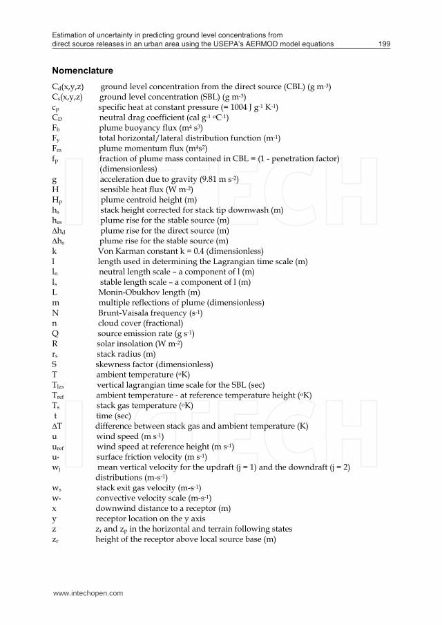
Estimation of uncertainty in predicting ground level concentrations from direct source releases in an urban area using the USEPA’s AERMOD model equations 199

Rao, S.K. Uncertainty analysis in atmospheric dispersion modeling. Pure Appl. Geophys. 2005, 162, 1893-1917.

Rodriguez, M.A.; Brouwer, J.; Samuelsen, G.S.; Dabdub, D. Air quality impacts of distributed power generation in the south coast air basin of california 2: model uncertainty and sensitivity analysis. J. Atmos. Environ. 2007, 41, 5618–5635

Romano, D.; Bernetti, A.; De Lauretis, R. Different methodologies to quantify uncertainties of Air Emissions. Environ. Int. 2004, 30, 1099-1107

Rubinstein, R.Y. (1981). Simulation and the Monte Carlo Method. John Wiley & Sons. Sathyajith, M.; Pandey, K.P.; Kumar, A.V. Analysis of wind regimes for energy estimation.

Renew. Energ. 2002, 25, 381-399. Sax, T.; Isakov, V. A case Study for assessing uncertainty in local scale regulatory air quality

modeling applications. J. Atmos. Environ. 2003, 37, 3481-3489 Scavia, D.; Powers, W.F.; Canale, R.P.; Moody, J.L. Comparison of first-order error analysis

and monte carlo simulation in time-dependent lake eutrophication models. Water. Resour. Res. 1981, 17, 1051-1059.

Seigneur, C.; Constantinou, E.; Permutt, T. Uncertainty analysis of health risk estimates. Document No. 2460-009-510, Electric Power Research Institute, Palo Alto, California, 1992.

Shafer, G. (1976). A mathematical theory of evidence. New Jersey: Princeton Univ. Press. Smith, R.I.; Fowler, D.; Sutton, M.A.; Flechard, C.; Coyle, M. Regional estimation of

pollutant gas dry deposition in the UK: model description, sensitivity analyses and outputs. J. Atmos. Environ. 2000, 34, 3757–3777.

Thomas, S.T.; Kumar, A.; Vangipuram, R.N. Sensitivity analysis of a statistical type long range transport model. Paper No. 85-5.8. 78th Annual Meeting of Air Pollution Control Association. June 1985.

Vardoulakis, S.; Fisher, B.E.A.; Gonzalez-Flesca, N.; Pericleous, K. Model sensitivity and uncertainty analysis using roadside air quality measurements. J. Atmos. Environ. 2002, 36, 2121-2134.

Venkatram, A.; Strimaitis, D.G.; Dicristofaro, D. A semiemperical model to estimate vertical dispersion of eleveated releases in the stable boundary layer. J. Atmos. Environ. 1984, 18, 923-928

Vuilleumier, L.; Bamer, J.T.; Harley, R.A.; Brown, N.J. Evaluation of nitrogen dioxide photolysis rates in an urban area using data from the 1997 southern california ozone study. J. Atmos. Environ. 2001, 35, 6525–6537.

Weil, J.C.; Corio, L.A.; Brower, R.P. A PDF dispersion model for buoyant plumes in the convective boundary layer. J. Appl Meteorol. 1997, 36, 982-1002.

Willis, G.E.; Deardroff, J.W. A laboratory study of dispersion in the middle of the convectively mixed layer. J. Atmos. Environ. 1981, 15, 109-117.

Worley, B.A. (1987). Deterministic uncertainty analysis. ORNL-6428. Oak Ridge National Laboratory, Oak Ridge, Tennessee.

Yang, Y.J.; Wilkinson, J.G.; Russell, A.G. Fast, direct sensitivity analysis of multidimensional models. J. Environ. Sci. Technol. 1997, 31, 2859–2868.

Yegnan, A.; Williamson, D.G.; Graettinger, A.J. Uncertainty analysis in air dispersion modeling. J. Environ. Modell. Softw. 2002, 17, 639-649.

Zadeh, L. Fuzzy sets as a basis for a theory of possibility. Fuzzy. Set. Syst. 1978, 1, 3-28.

Nomenclature Cd(x,y,z) ground level concentration from the direct source (CBL) (g m-3) Cs(x,y,z) ground level concentration (SBL) (g m-3) cp specific heat at constant pressure (= 1004 J g-1 K-1) CD neutral drag coefficient (cal g-1 oC-1) Fb plume buoyancy flux (m4 s3) Fy total horizontal/lateral distribution function (m-1) Fm plume momentum flux (m4s2) fp fraction of plume mass contained in CBL = (1 - penetration factor) (dimensionless) g acceleration due to gravity (9.81 m s-2) H sensible heat flux (W m-2) Hp plume centroid height (m) hs stack height corrected for stack tip downwash (m) hes plume rise for the stable source (m) ∆hd plume rise for the direct source (m) ∆hs plume rise for the stable source (m) k Von Karman constant k = 0.4 (dimensionless) l length used in determining the Lagrangian time scale (m) ln neutral length scale – a component of l (m) ls stable length scale – a component of l (m) L Monin-Obukhov length (m) m multiple reflections of plume (dimensionless) N Brunt-Vaisala frequency (s-1) n cloud cover (fractional) Q source emission rate (g s-1) R solar insolation (W m-2) rs stack radius (m) S skewness factor (dimensionless) T ambient temperature (oK) Tlzs vertical lagrangian time scale for the SBL (sec) Tref ambient temperature - at reference temperature height (oK) Ts stack gas temperature (oK) t time (sec) ∆T difference between stack gas and ambient temperature (K) u wind speed (m s-1) uref wind speed at reference height (m s-1) u* surface friction velocity (m s-1) wj mean vertical velocity for the updraft (j = 1) and the downdraft (j = 2) distributions (m-s-1) ws stack exit gas velocity (m-s-1) w* convective velocity scale (m-s-1) x downwind distance to a receptor (m) y receptor location on the y axis z zr and zp in the horizontal and terrain following states zr height of the receptor above local source base (m)

www.intechopen.com

Air Quality200

zp receptor “flagpole” height - the height of a receptor above local terrain (m) zi mixing height (m): zi = MAX [zic; zim] in the CBL and zi = zim in the SBL zic convective mixing height (m) zie equilibrium height of stable boundary layer zieff height of the reflecting surface in the SBL or in the stable layer above the CBL (m) zim mechanical mixing height (m) zo surface roughness length (m) (0.03 m for open flat terrain, grass, few obstacles; 1 m for more obstacles) zref reference height for wind (m) θ potential temperature (oK) θ* temperature scale (oK) λj weighting coefficient for the updraft (j = 1) and downdraft (j = 2) distributions ρ density of air (Kg m-3) σv lateral turbulence (m s-1) σwt total vertical turbulence (m s-1) σy total lateral dispersion parameter for the direct source (m) σz total vertical dispersion parameter for the direct source (m) σzas ambient dispersion for the stable source (m) σzes elevated portion of σzas (m) σzgs surface portion of σzas (m) σzj total vertical dispersion for the updrafts and downdrafts (j=1, 2 respectively) σzs total dispersion for the stable source (m) τ time constant controlling the temporal interpolation of zim (sec) ψdj total height of the direct source plume (i.e. release height + buoyancy +

convection) (m) βm 5

height of the direct source plume

www.intechopen.com

Air QualityEdited by Ashok Kumar

ISBN 978-953-307-131-2Hard cover, 382 pagesPublisher SciyoPublished online 18, August, 2010Published in print edition August, 2010

InTech EuropeUniversity Campus STeP Ri Slavka Krautzeka 83/A 51000 Rijeka, Croatia Phone: +385 (51) 770 447 Fax: +385 (51) 686 166www.intechopen.com

InTech ChinaUnit 405, Office Block, Hotel Equatorial Shanghai No.65, Yan An Road (West), Shanghai, 200040, China

Phone: +86-21-62489820 Fax: +86-21-62489821

Air pollution is about five decades or so old field and continues to be a global concern. Therefore, thegovernments around the world are involved in managing air quality in their countries for the welfare of theircitizens. The management of air pollution involves understanding air pollution sources, monitoring ofcontaminants, modeling air quality, performing laboratory experiments, the use of satellite images forquantifying air quality levels, indoor air pollution, and elimination of contaminants through control. Researchactivities are being performed on every aspect of air pollution throughout the world, in order to respond topublic concerns. The book is grouped in five different sections. Some topics are more detailed than others.The readers should be aware that multi-authored books have difficulty maintaining consistency. A reader willfind, however, that each chapter is intellectually stimulating. Our goal was to provide current information andpresent a reasonable analysis of air quality data compiled by knowledgeable professionals in the field of airpollution.

How to referenceIn order to correctly reference this scholarly work, feel free to copy and paste the following:

Vamsidhar V. Poosarala, Ashok Kumar and Akhil Kadiyala (2010). Estimation of Uncertainty in PredictingGround Level Concentrations from Direct Source Releases in an Urban Area Using the USEPA’s AERMODModel Equations, Air Quality, Ashok Kumar (Ed.), ISBN: 978-953-307-131-2, InTech, Available from:http://www.intechopen.com/books/air-quality/estimation-of-uncertainty-in-predicting-ground-level-concentrations-from-direct-source-releases-in-a