9.1 t he no slip condition - stanford universitycantwell/aa200_course_material/aa200... · 9.1 t he...
TRANSCRIPT

bjc 9.1 5/8/13
C
HAPTER
9 V
ISCOUS
F
LOW
A
LONG
A W
ALL
9.1 T
HE
NO
-
SLIP
CONDITION
All liquids and gases are viscous and, as a consequence, a fluid near a solid bound-ary sticks to the boundary. The tendency for a liquid or gas to stick to a wall arisesfrom momentum exchanged during molecular collisions with the wall. Viscousfriction profoundly changes the fluid flow over a body compared to the ideal invis-cid approximation that is widely applied in aerodynamic theory. The figure belowillustrates the effect in the flow over a curved boundary. Later we will see how thevelocity at the wall from irrotational flow theory is used as the outer boundary
condition for the equations that govern the thin region of rotational flow near thewall imposed by the no-slip condition. This thin layer is called a boundary layer.
Figure 9.1 Slip versus no-slip flow near a solid surface.
The presence of low speed flow near the surface of a wing can lead to flow sepa-ration or stall. Separation can produce large changes in the pressure fieldsurrounding the body leading to a decrease in lift and an increase in pressurerelated drag. The pressure drag due to stall may be much larger than the drag dueto skin friction. In a supersonic flow the no-slip condition insures that there isalways a subsonic flow near the wall enabling pressure disturbances to propagateupstream through the boundary layer. This may cause flow separation and shockformation leading to increased wave drag.
In Appendix 1 we worked out the mean free path between collisions in a gas
Ue
UeUe

The no-slip condition
5/8/13 9.2 bjc
(9.1)
where is the number of molecules per unit volume and is the collision diam-eter of the molecule. On an atomic scale all solid materials are rough and adsorbor retard gas molecules near the surface. When a gas molecule collides with a solidsurface a certain fraction of its momentum parallel to the surface is lost due to Vander Walls forces and interpenetration of electron clouds with the molecules at thesolid surface. Collisions of a rebounding gas molecule with other gas moleculeswithin a few mean free paths of the surface will slow those molecules and causethe original molecule to collide multiple times with the surface. Within a few col-lision times further loss of tangential momentum will drop the average molecularvelocity to zero. At equilibrium, the velocity of the gas within a small fraction ofa mean free path of the surface and the velocity of the surface must match.
The exception to this occurs in the flow of a rarified gas where the distance a mol-ecule travels after a collision with the surface is so large that a return to the surfacemay never occur and equilibrium is never established. In this case there is a slipvelocity that can be modeled as
(9.2)
where is a constant of order one. The slip velocity is negligible for typical val-ues of the mean free path in gases of ordinary density. In situations where thevelocity gradient is extremely large as in some gas lubrication flows there can besignificant slip even at ordinary densities.
For similar reasons there can be a discontinuity in temperature between the walland gas in rarified flows or very high shear rate flows.
In this Chapter we will discuss two fundamental problems involving viscous flowalong a wall at ordinary density and shear rate. The first is plane Couette flowbetween two parallel plates where the flow is perfectly parallel. This problem canbe solved exactly. The second is the plane boundary layer along a wall where theflow is almost but not quite perfectly parallel. In this case an approximate solutionto the equations of motion can be determined.
1
2 n 2---------------------=
n
vslip C Uy
-------=
C

Equations of Motion
bjc 9.3 5/8/13
9.2 E
QUATIONS
OF
M
OTION
Recall the equations of motion in Cartesian coordinates from Chapter 1, in theabsence of body forces and internal sources of energy.
. . (9.3)
The first simplification is to reduce the problem to steady flow in two spacedimensions.
Conservation of mass
t------ U
x----------- V
y----------- W
z------------+ + + 0=
Conservation of momentum
Ut
-----------UU P xx–+( )
x----------------------------------------------
UV xy–( )
y-----------------------------------
UW xz–( )
z------------------------------------+ + + 0=
Vt
-----------VU xy–( )
x-----------------------------------
VV P yy–+( )
y---------------------------------------------
VW yz–( )
z-----------------------------------+ + + 0=
Wt
------------WU xz–( )
x------------------------------------
WV yz–( )
y-----------------------------------
WW P zz–+( )
z-----------------------------------------------+ + + 0=
Conservation of energy
et
---------hU Qx+( )
x----------------------------------
hV Qy+( )
y---------------------------------
hW Qz+( )
z---------------------------------- –+ + +
U Px
------- V Py
------- W Pz
-------+ + xxUx
------- xyUy
------- xzUz
-------+ +– –
xyVx
------- yyVy
------- yzVz
-------+ + xzWx
-------- yzWy
-------- zzWz
--------+ +– 0=

Plane, Compressible, Couette Flow
5/8/13 9.4 bjc
(9.4)
9.3 PLANE, COMPRESSIBLE, COUETTE FLOW
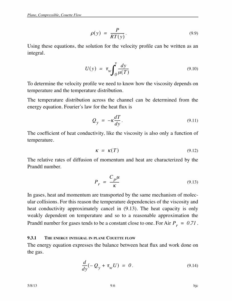
First let’s study the two-dimensional, compressible flow produced between twoparallel plates in relative motion shown below. This is the simplest possible com-pressible flow where viscous forces and heat conduction dominate the motion. Westudied the incompressible version of this flow in Chapter 1. There the gas tem-perature is constant and the velocity profile is a straight line. In the compressibleproblem the temperature varies substantially, as does the gas viscosity, leading toa more complex and more interesting problem.
Figure 9.2 Flow produced between two parallel plates in relative motion
Ux
----------- Vy
-----------+ 0=
UU P xx–+( )
x---------------------------------------------
UV xy–( )
y-----------------------------------+ 0=
VU xy–( )
x----------------------------------
VV P yy–+( )
y--------------------------------------------+ 0=
hU Qx+( )
x---------------------------------
hV Qy+( )
y--------------------------------- U P
x------- V P
y-------+–+
xxUx
------- xyUy
-------+– xyVx
------- yyVy
-------+ – 0=
U(y)
x
y
UT
w Tw Qw
d

Plane, Compressible, Couette Flow
bjc 9.5 5/8/13
The upper wall moves at a velocity doing work on the fluid while the lower
wall is at rest. The temperature of the upper wall is . The flow is assumed to
be steady with no variation in the direction. The plates extend to plus and minusinfinity in the direction.
All gradients in the direction are zero and the velocity in the direction is zero.
(9.5)
With these simplifications the equations of motion simplify to
. (9.6)
The velocity component and temperature only depend on . The momentumequation implies that the pressure is uniform throughout the flow (the pressuredoes not depend on or ). The implication of the momentum balance is thatthe shear stress also must be uniform throughout the flow just like the pres-
sure. Assume the fluid is Newtonian. With , the shear stress is
(9.7)
where is the shear stress at the lower wall. For gases the viscosity depends
only on temperature.
(9.8)
Since the pressure is constant the density also depends only on the temperature.According to the perfect gas law
U
T
zx
x y
V W 0= =
x------ ( ) z
----- ( ) 0= =
xyy
----------- 0=
Py
------- 0=
Qy xy– U( )
y------------------------------- 0=
U y y
x y x
xy
V 0=
xy µ yddU
w cons ttan= = =
w
µ µ T( )=
Plane, Compressible, Couette Flow
5/8/13 9.6 bjc
. (9.9)
Using these equations, the solution for the velocity profile can be written as anintegral.
(9.10)
To determine the velocity profile we need to know how the viscosity depends ontemperature and the temperature distribution.
The temperature distribution across the channel can be determined from theenergy equation. Fourier’s law for the heat flux is
. (9.11)
The coefficient of heat conductivity, like the viscosity is also only a function oftemperature.
(9.12)
The relative rates of diffusion of momentum and heat are characterized by thePrandtl number.
(9.13)
In gases, heat and momentum are transported by the same mechanism of molec-ular collisions. For this reason the temperature dependencies of the viscosity andheat conductivity approximately cancel in (9.13). The heat capacity is onlyweakly dependent on temperature and so to a reasonable approximation thePrandtl number for gases tends to be a constant close to one. For Air .
9.3.1 THE ENERGY INTEGRAL IN PLANE COUETTE FLOW
The energy equation expresses the balance between heat flux and work done onthe gas.
. (9.14)
y( ) PRT y( )----------------=
U y( ) wdyµ T( )------------
0
y=
QydTdy-------–=
T( )=
PrC pµ-----------=
Pr 0.71=
ddy------ Qy– wU+( ) 0=
Plane, Compressible, Couette Flow
bjc 9.7 5/8/13
Integrate (9.14).
(9.15)
The constant of integration, , is the heat flux on the lower
wall. Now insert the expressions for the shear stress and heat flux into (9.15).
(9.16)
Integrate (9.16) from the lower wall.
(9.17)
is the temperature of the lower wall. The integral on the right of (9.17) can be
replaced by the velocity using (9.10). The result is the so-called energy integral.
(9.18)
At the upper wall, the temperature is and this can now be used to evaluate the
lower wall temperature.
(9.19)
9.3.2 THE ADIABATIC WALL RECOVERY TEMPERATURE
Suppose the lower wall is insulated so that . What temperature does the
lower wall reach? This is called the adiabatic wall recovery temperature .
(9.20)
Introduce the Mach number . Now
Qy– wU+ Qw–=
Qw T y( )y 0==
kdTdy------- µU dU
dy-------+ µ
ddy------ 1
Pr------C pT 1
2---U2+ Qw–= =
C p T T w–( )12---PrU2+ QwPr
dyµ T( )------------
0
y–=
T w
C p T T w–( )12---PrU2+
Qw
w--------PrU–=
T
C pT w C pT PrU 2
2-----------
Qw
w--------U++=
Qw 0=
T wa
T wa TPr
2C p----------U 2+=
M U a=

Plane, Compressible, Couette Flow
5/8/13 9.8 bjc
. (9.21)
Equation (9.21) indicates that the recovery temperature equals the stagnation tem-perature at the upper wall only for a Prandtl number of one. The stagnationtemperature at the upper wall is
. (9.22)
The recovery factor is defined as
. (9.23)
In Couette flow for a perfect gas with constant (9.21) tells us that the recovery
factor is the Prandtl number.
(9.24)
Equations (9.19) and (9.20) can be used to show that the heat transfer and shearstress are related by
. (9.25)
Equation (9.25) can be rearranged to read
. (9.26)
The left side of (9.26) is the friction coefficient
. (9.27)
T waT---------- 1 Pr
1–2
------------ M 2+=
T t
T-------- 1 1–
2------------ M 2+=
T wa T–T t T–------------------------ r=
C p
T wa T–T t T–------------------------ Pr=
Qw
wU---------------
C p T w T wa–( )
PrU2------------------------------------=
w12--- U2------------------- 2Pr
QwU C p T w T wa–( )
-----------------------------------------------------=
C fw
12--- U2-------------------=

Plane, Compressible, Couette Flow
bjc 9.9 5/8/13
On the right side of (9.26) there appears a dimensionless heat transfer coefficientcalled the Stanton number.
(9.28)
In order to transfer heat into the fluid the lower wall temperature must exceed therecovery temperature. Equation (9.26) now becomes
. (9.29)
The coupling between heat transfer and viscous friction indicated in (9.29) is ageneral property of all compressible flows near a wall. The numerical factor may change and the dependence on Prandtl number may change depending on theflow geometry and on whether the flow is laminar or turbulent, but the generalproperty that heat transfer affects the viscous friction is universal.
9.3.3 VELOCITY DISTRIBUTION IN COUETTE FLOW
Now that the relation between temperature and velocity is known we can integratethe momentum relation for the stress. We use the energy integral written in termsof
(9.30)
or
. (9.31)
Recall the momentum equation.
(9.32)
The temperature is a monotonic function of the velocity and so the viscosity canbe regarded as a function of . This enables the momentum equation to beintegrated.
StQw
U C p T w T wa–( )-----------------------------------------------------=
C f 2PrSt=
2
T
C p T T–( ) PrQw
w-------- U U–( )
12---Pr U 2 U2–( )+=
TT------- 1 Pr
QwU w--------------- 1–( )M2 1 U
U--------– Pr
1–2
------------ M2 1 U2
U 2-----------–+ +=
µ T( ) yddU
w=
U

Plane, Compressible, Couette Flow
5/8/13 9.10 bjc
(9.33)
In gases, the dependence of viscosity on temperature is reasonably well approxi-mated by Sutherland’s law.
(9.34)
where is the Sutherland reference temperature which is for Air. An
approximation that is often used is the power law.
(9.35)
Using (9.31) and (9.35), the momentum equation becomes
(9.36)
For Air the exponent, , is approximately . The simplest case, and a reason-able approximation, corresponds to . In this case the integral can becarried out explicitly. For an adiabatic wall, the wall stress and velocity
are related by
. (9.37)
The shear stress is determined by evaluating (9.37) at the upper wall.
(9.38)
The velocity profile is expressed implicitly as
µ U( ) Ud0
U
wy=
µµ------- T
T-------
3 2 T T S+T T S+
---------------------=
T S 110.4K
µµ------- T
T-------= 0.5 1.0< <
1 PrQw
U w--------------- 1–( )M2 1 U
U--------– Pr
1–2
------------ M2 1 U2
U 2-----------–+ + Ud
0
U wµ------- y=
0.761=Qw 0=
wµ U----------------y U
U-------- Pr
1–2
------------ M2 UU-------- 1
3--- U
U--------
3–+=
wµ U----------------d 1 Pr
1–3
------------ M2+=

Plane, Compressible, Couette Flow
bjc 9.11 5/8/13
. (9.39)
At the profile reduces to the incompressible limit . At
high Mach number the profile is
. (9.40)
At high Mach number the profile is independent of the Prandtl number and Machnumber. The two limiting cases are shown below.
Figure 9.3 Velocity distribution in plane Couette flow for an adiabatic lower wall and .
Using (9.38) the wall friction coefficient for an adiabatic lower wall is expressedin terms of the Prandtl, Reynolds and Mach numbers.
(9.41)
where the Reynolds number is
yd---
UU-------- Pr
1–2
------------ M2 UU-------- 1
3--- U
U--------
3–+
1 Pr1–
3------------ M2+
-----------------------------------------------------------------------------------------=
M 0 U U y d=
yd---
Mlim 3
2--- U
U-------- 1
3--- U
U--------
3–=
1=
C f 21 Pr
1–3
------------ M2+
Re--------------------------------------------=
The viscous boundary layer on a wall
5/8/13 9.12 bjc
(9.42)
The Reynolds number can be expressed as
. (9.43)
Here the interpretation of the Reynolds number as a ratio of convective to viscousforces is nicely illustrated.
Notice that if the upper and lower walls are both adiabatic the work done by theupper wall would lead to a continuous accumulation of energy between the twoplates and a continuous rise in temperature. In this case a steady state solution tothe problem would not exist. The upper wall has to be able to conduct heat intoor out of the flow for a steady state solution to be possible.
9.4 THE VISCOUS BOUNDARY LAYER ON A WALL
The Couette problem provides a useful insight into the nature of compressibleflow near a solid boundary. From a practical standpoint the more important prob-lem is that of a compressible boundary layer where the flow originates at theleading edge of a solid body such as an airfoil. A key reference is the classic textBoundary Layer Theory by Hermann Schlichting. Recent editions are authoredby Schlichting and Gersten.
To introduce the boundary layer concept we will begin by considering viscous,compressible flow past a flat plate of length shown in Figure 9.4. The questionof whether a boundary layer is present or not depends on the overall Reynoldsnumber of the flow.
(9.44)
Figure 9.4 depicts the case where the thickness of the viscous region, delineated,schematically by the parabolic boundary, is a significant fraction of the length ofthe plate and the Reynolds number based on the plate length is quite low.
ReU dµ
-------------------=
ReU dµ
-------------------
12--- U2
12---µ
Ud
---------------------------- dynamic pressure at the upper plate
characteristic shear stress--------------------------------------------------------------------------------------= = =
L
ReLU Lµ
-------------------=

The viscous boundary layer on a wall
bjc 9.13 5/8/13
In this case there is no boundary layer and the full equations of motion must besolved to determine the flow.
Figure 9.4 Low Reynolds number flow about a thin flat plate of length L. is less than a hundred or so. The parabolic envelope which extends
upstream of the leading edge roughly delineates the region of rotational flow produced as a consequence of the no slip condition on the plate.
If the Reynolds number based on plate length is large then the flow looks morelike that depicted in Figure 9.5.
Figure 9.5 High Reynolds number flow developing from the leading edge of a flat plate of length L. is several hundred or more.
U(y)
x
y
UT
wTw Qw
P
L
ReL
U(y)
x
y
UT
wTw Qw
Ue(x),
P
L
Te(x), Pe(x)
ReL

The viscous boundary layer on a wall
5/8/13 9.14 bjc
At high Reynolds number the thickness of the viscous region is much less thanthe length of the plate.
(9.45)
Moreover, there is a region of the flow away from the leading and trailing edgesof the plate where the guiding effect of the plate produces a flow that is nearlyparallel. In this region the transverse velocity component is much less than thestreamwise component.
(9.46)
The variation of the flow in the streamwise direction is much smaller than the vari-ation in the cross-stream direction. Thus
. (9.47)
Moreover continuity tells us that
. (9.48)
The convective and viscous terms in the streamwise momentum equation are ofthe same order suggesting the following estimate for .
(9.49)
With this estimate in mind let’s examine the momentum equation.
(9.50)
Utilizing (9.46) and (9.47), equation (9.50) reduces to
. (9.51)
L--- 1«
VU---- 1«
( )x
--------- ( )y
---------« U ( )x
--------- V ( )y
---------
Ux
------- Vy
-------–
L
U 2
L------------------ µ
U2--------
L--- 1
ReL( )1 2-----------------------
y
VU xy–( )
x----------------------------------
VV P yy–+( )
y--------------------------------------------+ 0=
P yy–( )
y-------------------------- 0=

The viscous boundary layer on a wall
bjc 9.15 5/8/13
Now integrate this equation at a fixed position and evaluate the constant of inte-gration in the free stream.
(9.52)
The pressure (9.52) is inserted into the momentum equation in (9.4). The resultis the boundary layer approximation to the momentum equation.
(9.53)
Now consider the energy equation.
(9.54)
Using (9.46), (9.47) and (9.48) the energy equation simplifies to
. (9.55)
In laminar flow the normal stresses and are very small and the normal
stress terms that appear in (9.53) and (9.55) can be neglected. In turbulent flowthe normal stresses are not particularly small, with fluctuations of velocity nearthe wall that can be percent of the velocity at the edge of the boundarylayer. Nevertheless a couple of features of the turbulent boundary layer (com-pressible or incompressible) allow these normal stress terms in the boundary layerequations to be neglected.
x
P x y,( ) yy x y,( ) Pe x( )+=
xx
U Ux
------- V Uy
-------+dPedx
---------– x------ xx yy–( ) xy
y-----------+ +=
hU Qx+( )
x---------------------------------
hV Qy+( )
y--------------------------------- –+
U Px
------- V Py
-------+ xxUx
------- xyUy
-------+– –
xyVx
------- yyVy
-------+ 0=
U hx
------ V hy
------Qyy
---------- UdPedx
---------– U x------ xx yy–( ) –+ + +
V yy( )
y--------------------
U xx( )
x---------------------– xy
Uy
-------– 0=
xx yy
10 20–

The viscous boundary layer on a wall
5/8/13 9.16 bjc
1) and tend to be comparable in magnitude so that is small and
the streamwise derivative is generally quite small.
2) has its maximum value in the lower part of the boundary layer where is
very small so the product is small.
3) also has its maximum value relatively near the wall where is relatively
small and the streamwise derivative of is small.
Using these assumptions to remove the normal stress terms, the compressibleboundary layer equations become
. (9.56)
The only stress component that plays a role in this approximation is the shearingstress . In a turbulent boundary layer both the laminar and turbulent shearing
stresses are important.
(9.57)
In the outer part of the layer where the velocity gradient is relatively small theturbulent stresses dominate, but near the wall where the velocity fluctuations aredamped and the velocity gradient is large, the viscous stress dominates.
The flow picture appropriate to the boundary layer approximation is shown below.
xx yy xx yy–
xx yy–( ) x
yy V
V yy
xx U
U xx
Ux
----------- Vy
-----------+ 0=
U Ux
------- V Uy
-------+dPedx
---------– xyy
-----------+=
U hx
------ V hy
------Qyy
---------- UdPedx
---------– xyUy
-------–+ + 0=
xy
xy xy laminar xy turbulent+ µ
Uy
------- xy turbulent+= =
The viscous boundary layer on a wall
bjc 9.17 5/8/13
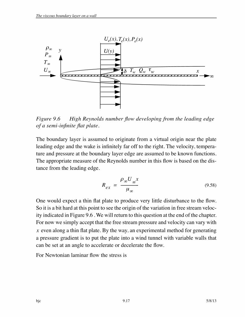
Figure 9.6 High Reynolds number flow developing from the leading edge of a semi-infinite flat plate.
The boundary layer is assumed to originate from a virtual origin near the plateleading edge and the wake is infinitely far off to the right. The velocity, tempera-ture and pressure at the boundary layer edge are assumed to be known functions.The appropriate measure of the Reynolds number in this flow is based on the dis-tance from the leading edge.
(9.58)
One would expect a thin flat plate to produce very little disturbance to the flow.So it is a bit hard at this point to see the origin of the variation in free stream veloc-ity indicated in Figure 9.6 . We will return to this question at the end of the chapter.For now we simply accept that the free stream pressure and velocity can vary with
even along a thin flat plate. By the way, an experimental method for generatinga pressure gradient is to put the plate into a wind tunnel with variable walls thatcan be set at an angle to accelerate or decelerate the flow.
For Newtonian laminar flow the stress is
U(y)
x
y
UT
wTw Qw
Ue(x),
P
Te(x), Pe(x)
Rex
U x
µ-------------------=
x

The viscous boundary layer on a wall
5/8/13 9.18 bjc
. (9.59)
The diffusion of heat is governed by Fourier’s law introduced earlier.
(9.60)
For laminar flow the compressible boundary layer equations are
. (9.61)
9.4.1 MEASURES OF BOUNDARY LAYER THICKNESS
The thickness of the boundary layer depicted in Figure 9.6 is denoted by . Thereare several ways to define the thickness. The simplest is to identify the point wherethe velocity is some percentage of the free stream value, say or . More
rigorous and in some ways more useful definitions are the following.
Displacement thickness
(9.62)
This is a measure of the distance by which streamlines are shifted away from theplate by the blocking effect of the boundary layer. This outward displacement ofthe flow comes from the reduced mass flux in the boundary layer compared to the
mass flux that would occur if the flow were inviscid. Generally is a fraction of. The integral (9.62) is terminated at the edge of the boundary layer where
ij 2µSij23---µ µv– ijSkk–=
xy µUy
------- Vx
-------+ µUy
-------=
QyTy
-------–=
Ux
----------- Vy
-----------+ 0=
U Ux
------- V Uy
-------+dPedx
---------– y------ µ
Uy
-------+=
UC pTx
------- V C pTy
-------+ UdPedx
---------y
------ Ty
------- µUy
-------2
+ +=
0.95 0.99
* 1 UeUe
-------------– yd0
=
*
0.99
The Von Karman integral momentum equation
bjc 9.19 5/8/13
the velocity equals the free stream value . This is important in a situation
involving a pressure gradient where the velocity profile might look something likethat depicted in Figure 9.1. The free stream velocity used as the outer boundarycondition for the boundary layer calculation comes from the potential flow solu-tion for the irrotational flow about the body evaluated at the wall. If the integral(9.62) is taken beyond this point it will begin to diverge.
Momentum thickness
(9.63)
This is a measure of the deficit in momentum flux within the boundary layer com-pared to the free stream value and is smaller than the displacement thickness. Theevolution of the momentum thickness along the wall is directly related to the skinfriction coefficient.
9.5 THE VON KARMAN INTEGRAL MOMENTUM EQUATION
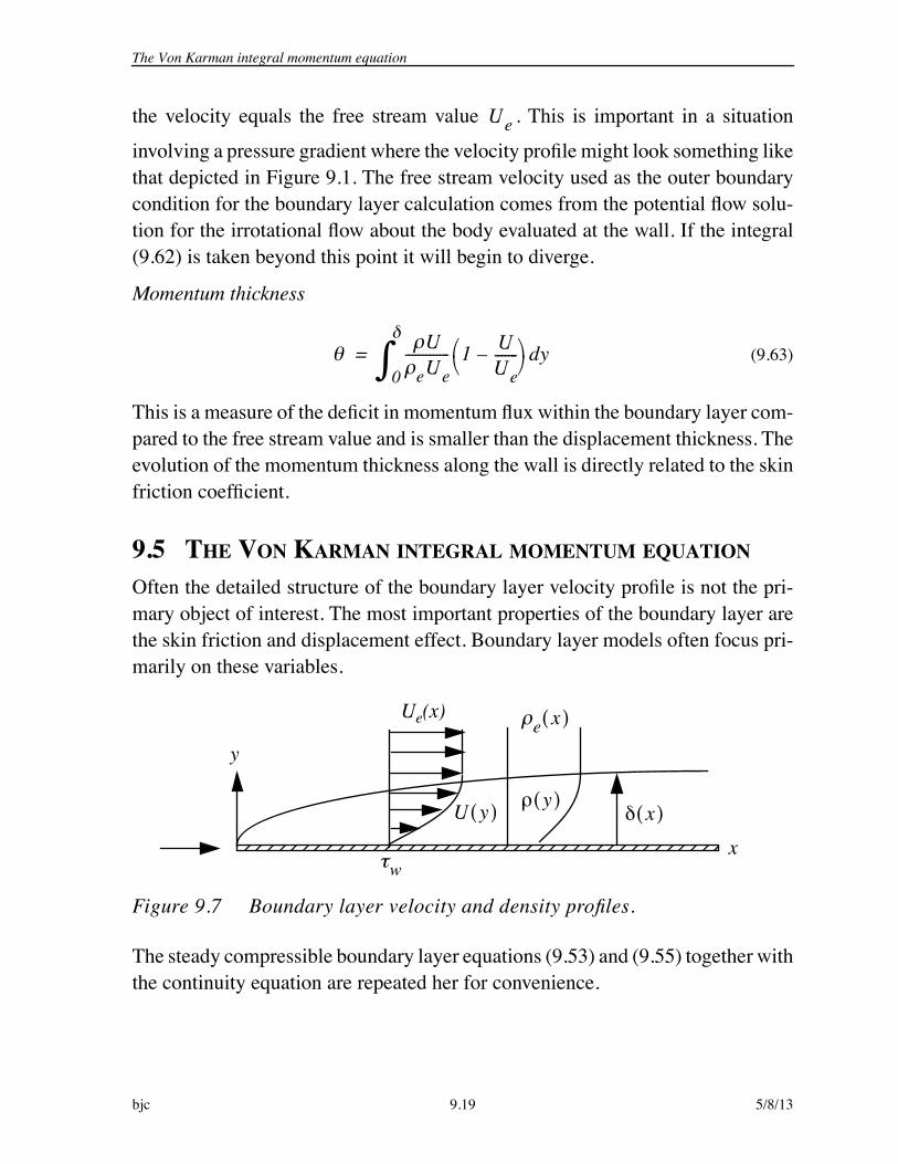
Often the detailed structure of the boundary layer velocity profile is not the pri-mary object of interest. The most important properties of the boundary layer arethe skin friction and displacement effect. Boundary layer models often focus pri-marily on these variables.
Figure 9.7 Boundary layer velocity and density profiles.
The steady compressible boundary layer equations (9.53) and (9.55) together withthe continuity equation are repeated her for convenience.
Ue
UeUe
------------- 1 UUe-------– yd
0=
x
y
w
Ue(x)e x( )
U y( )y( )
x( )

The Von Karman integral momentum equation
5/8/13 9.20 bjc
(9.64)
Integrate the continuity and momentum equations over the thickness of theboundary layer.
(9.65)
Upon integration the momentum equation becomes
(9.66)
The partial derivatives with respect to in (9.64) can be taken outside the integralusing Liebniz’ rule.
(9.67)
Use the second equation in (9.67) in (9.66).
(9.68)
where and is positive. We will make use of the follow-
ing relation.
Ux
----------- Vy
-----------+ 0=
U2
x-------------- UV
y---------------+
dPedx
---------– xyy
-----------+=
Ux
----------- yd0
x( ) Vy
----------- yd0
x( )+ 0=
U2
x-------------- yd
0
x( ) UVy
---------------- yd0
x( )+
dPedx
--------- yd0
x( )– xy
y----------- yd
0
x( )+=
U2
x-------------- yd
0
x( )
eUeV e+dPedx
--------- x( )– xy y 0=+=
x
ddx------ U yd
0
x( ) Ux
----------- yd0
x( )
eUeddx------+=
ddx------ U2 yd
0
x( ) U2
x-------------- yd
0
x( )
eUe2d
dx------+=
ddx------ U2 yd
0
x( )
eUe2d
dx------– eUeV e
dPedx
--------- x( )+ + – w=
w x( ) – xy x 0,( )= w

The Von Karman integral momentum equation
bjc 9.21 5/8/13
(9.69)
Multiply the continuity equation in (9.65) by and integrate with respect to .
(9.70)
Insert (9.70) in the last relation in (9.69).
(9.71)
Subtract(9.71) from (9.68).
(9.72)
and subtract the identity
(9.73)
from (9.72). Now the integral momentum equation takes the form
(9.74)
Recall the definitions of displacement thickness (9.62) and momentum thickness(9.63).
ddx------ UUe yd
0
x( ) UUex
------------------- yd0
x( )
eUe2d
dx------+ = =
UeUx
----------- UdUedx
----------+ yd0
x( )
eUe2d
dx------+ =
UeUx
----------- yd0
x( ) dUedx
---------- U yd0
x( )
eUe2d
dx------+ +
Ue y
UeUx
----------- yd0
x( )
eUeV e+ 0=
ddx------ UUe yd
0
x( )
eUeV edUedx
---------- U yd0
x( )
eUe2d
dx------––+ 0=
ddx------ U2 UUe–( ) yd
0
x( ) dUedx
---------- U yd0
x( ) dPedx
--------- x( )+ + – w=
dUedx
---------- eUe yd0
x( )
eUedUedx
---------- x( )– 0=
ddx------ U2 UUe–( ) yd
0
x( ) dUedx
---------- U eUe–( ) yd0
x( ) + +
dPedx
--------- eUedUedx
----------+ x( ) – w=
The Von Karman integral momentum equation
5/8/13 9.22 bjc
(9.75)
Substitute (9.75) into (9.74). The result is
(9.76)
At the edge of the boundary layer both and go to zero and the -
boundary layer momentum equation reduces to the Euler equation.
(9.77)
Using (9.77), the integral equation (9.76) reduces to
(9.78)
The significance of this last step is that (9.78) does not depend explicitly on thepercieved boundary layer thickness but only on the more precisely definedmomentum and displacement thicknesses. It is customary to write (9.78) in aslightly different form. Introduce the wall friction coefficient and carry out the dif-ferentiation of the first term in (9.78).
(9.79)
The Von Karman integral momentum equation is
(9.80)
Another common form of (9.80) is generated by introducing the shape factor
(9.81)
* x( ) 1 UeUe
-------------– yd0
x( )=
x( )U
eUe------------- 1 U
Ue-------– yd
0
x( )=
ddx------ eUe
2( ) eUe
*dUedx
----------dPedx
--------- eUedUedx
----------+ x( )+ + w=
U y xy x
dPe eUedUe+ 0=
ddx------ eUe
2( ) eUe
*dUedx
----------+ w=
x( )
C fw
12--- eUe
2-----------------=
ddx------ 2 *+( )
1Ue-------
dUedx
----------+C f2
-------=
H*
-----=

The laminar boundary layer in the limit
bjc 9.23 5/8/13
and (9.80) becomes
(9.82)
Equation (9.82) is valid for laminar, turbulent, compressible and incompressibleflow.
9.6 THE LAMINAR BOUNDARY LAYER IN THE LIMIT At very low Mach number the density, is constant, temperature variationsthroughout the flow are very small and the boundary layer equations (9.61) reduceto their incompressible form.
(9.83)
where the kinematic viscosity has been introduced. The boundary con-ditions are
. (9.84)
The pressure at the edge of the boundary layer is determined using theBernoulli relation
. (9.85)
The stagnation pressure is constant in the irrotational flow outside the boundarylayer. The pressure at the boundary layer edge, , is assumed to be a given
function determined from a potential flow solution for the flow outside the bound-ary layer.
The continuity equation is satisfied identically by introducing a stream function.
ddx------ 2 H+( )Ue
-------dUedx
----------+C f2
-------=
M2 0
Ux
------- Vy
-------+ 0=
U Ux
------- V Uy
-------+ 1---dPedx
---------–2U
y2----------+=
µ =
U 0( ) V 0( ) 0= = U ( ) Ue=
y =
Pt Pe x( )12--- Ue x( )
2 1---dPedx
--------- UedUedx
----------–=+=
Pe x( )

The laminar boundary layer in the limit
5/8/13 9.24 bjc
(9.86)
In terms of the stream function, the governing momentum equation becomes athird-order partial differential equation.
(9.87)
9.6.1 THE ZERO PRESSURE GRADIENT, INCOMPRESSIBLE BOUNDARY LAYER
For the governing equation reduces to
. (9.88)
with boundary conditions
(9.89)
We can solve this problem using a symmetry arguement. Transform (9.88) usingthe following three parameter dilation Lie group.
(9.90)
Equation (9.88) transforms as follows.
(9.91)
Equation (9.88) is invariant under the group (9.90) if and only if . Theboundaries of the problem at the wall and at infinity are clearly invariant under(9.90).
(9.92)
The free stream boundary condition requires some care.
(9.93)
Uy
-------= Vx
-------–=
y xy x yy– UedUedx
---------- yyy+=
dUe dx 0=
y xy x yy– yyy=
x 0,( ) y x 0,( ) 0= = y x,( ) Ue=
x eax= y eby= ec=
˜ y ˜ x y ˜ x ˜ y y– ˜ y y y– e2c a– 2b–y xy x yy–( ) ec 3b– ˜ y y y( )– 0= =
c a b–=
y eby 0 y 0= = =
˜ x 0,( ) ec eax 0,( ) 0 x 0,( ) 0= = =
y˜ x 0,( ) ec b–
y eax 0,( ) 0 y x 0,( ) 0= = =
˜ y x,( ) ec b–y eax,( ) Ue= =

The laminar boundary layer in the limit
bjc 9.25 5/8/13
Invariance of the free stream boundary condition only holds if . So theproblem as a whole, equation and boundary conditions, is invariant under the one-parameter group
(9.94)
This process of showing that the problem is invariant under a Lie group is essen-tially a proof of the existence of a similarity solution to the problem. We canexpect that the solution of the problem will also be invariant under the same group(9.94). That is we can expect a solution of the form
(9.95)
The problem can be further simplified by using the parameters of the problem tonondimensionalize the similarity variables. Introduce
(9.96)
In terms of these variables the velocities are
. (9.97)
The Reynolds number in this flow is based on the distance from the leading edge,(9.58).
(9.98)
As the distance from the leading edge increases, the Reynolds number increases, decreases, and the boundary layer approximation becomes more and more
accurate. The vorticity in the boundary layer is
. (9.99)
The remaining derivatives that appear in (9.88) are
c b=
x e2bx= y eby= eb=
x------- F y
x-------=
2 U x( )1 2 F( )= y
U2 x---------
1 2=
UU-------- F= V
U-------- 2U x
---------------1 2
F F–( )=
RexU x-----------=
V U
Vx
------- Uy
------- UU2 x---------–
1 2F–=

The laminar boundary layer in the limit
5/8/13 9.26 bjc
. (9.100)
Substitute (9.97) and (9.100) into (9.88).
(9.101)
Canceling terms in (9.101) leads to the Blasius equation
(9.102)
subject to the boundary conditions
. (9.103)
The numerical solution of the Blasius equation is shown below.
Figure 9.8 Solution of the Blasius equation (9.102) for the streamfunction, velocity and stress (or vorticity) profile in a zero pressure gradient laminar boundary layer.
The friction coefficient derived from evaluating the velocity gradient at the wall is
xyU2x--------– F=
yy UU2 x---------
1 2F=
yyyU2
2 x---------F=
U FU2x--------– F U– 2U x
---------------1 2
F F–( ) UU2 x---------
1 2F
U2
2 x---------F=
F– F( ) F F–( )F+ F=
– F F FF– F F F–+ 0=
F FF+ 0=
F 0( ) 0= F 0( ) 0= F ( ) 1=

The laminar boundary layer in the limit
bjc 9.27 5/8/13
. (9.104)
The transverse velocity component at the edge of the layer is
. (9.105)
Notice that at a fixed value of this velocity does not diminish with vertical dis-tance from the plate which may seem a little suprising given our notion that theregion of flow disturbed by a body should be finite and the disturbance should dieaway. But remember that in the boundary layer approximation, the body is semi-infinite. In the real flow over a finite length plate where the boundary layer solu-tion only applies over a limited region, the disturbance produced by the plate doesdie off at infinity.
The various thickness measures of the Blasius boundary layer are
. (9.106)
In terms of the similarity variable, the edge of the boundary layer at is at
.
We can use (9.102) to get some insight into the legitimacy of the boundary layeridea whereby the flow is separated into a viscous region where the vorticity is non-zero and an inviscid region where the vorticity is zero as depicted in Figure 9.29.
The dimensionless vorticity (or shear stress) is given in (9.99). Let .
The Blasius equation (9.102) can be espressed as follows.
(9.107)
Integrate (9.107).
C fw
1 2( ) U2--------------------------- 0.664Rex
-------------= =
V eU-------- 0.8604
Rex----------------=
x
0.99x
------------ 4.906Rex
-------------= *
x------- 1.7208
Rex----------------=
x--- 0.664
Rex-------------=
0.99
e 4.906 2 3.469= =
F=
d------ Fd–=
The Falkner-Skan boundary layers
5/8/13 9.28 bjc
(9.108)
The dimensionless stream function, the left panel in Figure 9.8, can be representedby
. (9.109)
The limiting behavior of is where is a positive constant
related to the displacement thickness of the boundary layer. If we substitute(9.109) into (9.108) and integrate beyond the edge of the boundary layer the resultis
. (9.110)
Equation (9.110) indicates that the shearing stress and vorticity decay exponen-tially at the edge of the layer. This rapid drop-off is a key point because it supportsthe fundamental idea of the boundary layer concept of separating the flow intotwo distinct zones.
9.7 THE FALKNER-SKAN BOUNDARY LAYERS
Finally, we address the question of free stream velocity distributions that lead toother similarity solutions beside the Blasius solution. We again analyze the streamfunction equation
. (9.111)
Let
(9.112)
where has units
w------ e
Fd0
–
=
F( ) G( )–=
G G( )lim C1= C1
w------
e>
eG( )–( )d
0–
C2eC1
2
2------–
= =
y xy x yy– UedUedx
----------– yyy– 0=
Ue Mx=
M

The Falkner-Skan boundary layers
bjc 9.29 5/8/13
. (9.113)
Similarity solutions of (9.111) exist for the class of power law freestream velocitydistributions given by (9.112). This is the well-known Falkner-Skan family ofboundary layers and the exponent is the Falkner-Skan pressure gradientparameter.
The form of the similarity solution can be determined using a symmetry argue-ment similar to that used to solve the zero pressure gradient case. Insert (9.113)into (9.111). The governing equation becomes
(9.114)
Now transform (9.114) using a three parameter dilation Lie group.
(9.115)
Equation (9.114) transforms as
. (9.116)
Equation (9.116) is invariant under the group (9.115) if and only if
. (9.117)
The boundaries of the problem at the wall and at infinity are invariant under(9.115).
(9.118)
As in the case of the Blasius problem, the free stream boundary condition requiressome care.
(9.119)
M L1 – T=
y xy x yy– M2x2 1–( )
– yyy– 0=
x eax= y eby= ˜ ec=
˜ y ˜ x y ˜ x ˜ y y– M2x2 1–
– ˜ y y y– =
e2c a– 2b–y xy x yy–( ) e 2 1–( )a M2x
2 1–( ) ec 3b– ˜ y y y( )–– 0=
2c a– 2b– c 3b– 2 1–( )a= =
y eby 0 y 0= = =
˜ x 0,( ) ec eax 0,( ) 0 x 0,( ) 0= = =
y˜ x 0,( ) ec b–
y eax 0,( ) 0 y x 0,( ) 0= = =
˜ y x,( ) ec b–y eax,( ) e aMx= =
The Falkner-Skan boundary layers
5/8/13 9.30 bjc
The boundary condition at the outer edge of the boundary layer is invariant if andonly if
(9.120)
Solving (9.117) and (9.120) for and in terms of leads to the group
(9.121)
We can expect that the solution of the problem will be invariant under the group(9.121). That is we can expect a solution of the form
(9.122)
As in the Blasius problem we use and to nondimensionalize the problem.The similarity variables are,
. (9.123)
Upon substitution of (9.123) and (9.112), the streamfunction equation, (9.111)becomes,
(9.124)
Cancelling terms produces the Falkner-Skan equation,
(9.125)
c b– a=
a c b
x e2
1 –------------b
x= y eby= ˜ e1 +1 –-------------b
=
x
1 +2
-------------------------------- F y
x
1 –2
------------------------------=
M
M2------
12---
y
x x0+( )1 –( ) 2
------------------------------------------=
Fx x0+( )
1 +( ) 2 2 M( )1 2
---------------------------------------------------------------------=
x x0+( )2 1– F 1 +( )F 1 –( ) F–( ) –(
F 1 +( )F 1 –( ) F–( ) 2– F– ) 0=
F 1 +( )FF 2 F( )2– 2+ + 0=

The Falkner-Skan boundary layers
bjc 9.31 5/8/13
with boundary conditions,
(9.126)
Note that reduces (9.125) to the Blasius equation. It is fairly easy toreduce the order by one. The new variables are
(9.127)
Differentiate
(9.128)
and
(9.129)
where the Falkner-Skan equation (9.125) has been used to replace the third deriv-ative. Equation (9.129) can be rearranged to read
. (9.130)
with the boundary conditions
. (9.131)
F 0[ ] 0 ; F 0[ ] 0 ; F [ ] 1= = =
0=
F ; G F= =
DGD---------
DD----------------- dG
d-------
G-------d GF
-------dF GF
----------dF+ +
-------d F-------dF+
--------------------------------------------------------------------FF
----------= = =
d2G
d 2----------
F F F2–
F2--------------------------------------- 1
F------- = =
F 1 +( )FF– 2 F( )2 2–+( ) F2–
F3---------------------------------------------------------------------------------------------------------------
GG 1 +( ) G G( )2 2 1
G---- G–+ + + 0=
G 0[ ] 0 ; G[ ] 1= =

The Falkner-Skan boundary layers
5/8/13 9.32 bjc
Several velocity profiles are shown in Figure 9.9.
Figure 9.9 Falkner-Skan velocity profiles
The various measures of boundary layer thickness including shape factor (9.81),and wall stress are shown below.
Figure 9.10 Falkner Skan boundary layer parameters versus .
1 2 3 4 5 60
0.2
0.4
0.6
0.8
1F
0=
0.5=
0.1=
0.07–=
0.0904–=(zero shear stress)
The Falkner-Skan boundary layers
bjc 9.33 5/8/13
9.7.1 THE CASE
A particularly interesting case occurs when . The pressure gradient termis,
(9.132)
and the original variables become,
. (9.133)
The units of the governing parameter, , are the same as the kinematicviscosity and so the ratio is the (constant) Reynolds number for the
flow. The governing equation becomes
(9.134)
The quantity is an area flow rate and can change sign depending on whetherthe flow is created by a source or a sink. The plus sign corresponds to a sourcewhile the minus sign represents a sink. To avoid an imaginary root, the absolutevalue of is used to nondimensionalize the stream function in (9.133). The oncereduced equation is
(9.135)
where
. (9.136)
Choose new variables
. (9.137)
1–=1–=
UeMx----- = Ue
dUedx
---------- M2
x3--------–=
2M
-------- yx x0+---------------=
F2 M( )
1 2-----------------------------±=
M L2 T=M
1–=
F 2 F( )2 2–( )± 0=
M
M
G2G GG 2 2 G2 1–( )±+ 0=
F ; G F= =
G ; H G= =

The Falkner-Skan boundary layers
5/8/13 9.34 bjc
Differentiate the new variables in (9.137) with respect to and divide.
. (9.138)
Equation (9.135) finally reduces to,
. (9.139)
9.7.2 FALKNER-SKAN SINK FLOW
At this point we will restrict ourselves to the case of a sink flow (choose the minussign in (9.135) and the plus sign in (9.139)). The flow we are considering issketched below.
Figure 9.11 Falkner-Skan sink flow for .
The negative sign in front of the in (9.133) insures that the velocity derived fromthe stream function is directed in the negative direction. The first order ODE,(9.139) (with the minus sign selected) can be broken into the autonomous pair,
(9.140)
dHd-------
H HGdGd------- HG
dGd
----------+ +
GdGd-------+
-------------------------------------------------------------GG
----------
G( )2
G---------------– 2
G2-------– 2+
G--------------------------------------------= = =
dHd------- H2 2 2 2–( )±–
2H-------------------------------------------=
x
y
1–=
Fx
dHds------- H2– 2– 2 2+=
dds------ 2H=

The Falkner-Skan boundary layers
bjc 9.35 5/8/13
with critical points at . The phase portrait of (9.140) is shownbelow.
Figure 9.12 Phase portrait of the Falkner Skan case .
Equation (9.139) is rearranged to read,
(9.141)
which, by the cross derivative test can be shown to be a perfect differential withthe integral,
. (9.142)
Recall that,
. (9.143)
At the edge of the boundary layer,
H,( ) 0 1±,( )=
-2 -1 1 2
-2
-1
1
2H
1–=
H2 2 2 2–+( )d 2H( )dH+ 0=
C 2 23--- 3– 1
2--- 2H2+=
G F= =
H GFF
----------= =

The Falkner-Skan boundary layers
5/8/13 9.36 bjc
. (9.144)
This allows us to evaluate in (9.142). The result is,
. (9.145)
Solve (9.142) for ,
(9.146)
where the positive root is recognized to be the physical solution. The solution(9.146) is shown as the thicker weight trajectory in Figure 9.12. Equation (9.146)can be written as,
(9.147)
In terms of the original variables
(9.148)
and
(9.149)
The latter result can be solved for the negative of the velocity, .
(9.150)
Flim 1=
Flim 0=H 1[ ] 0=
C
C 43---=
H
H 43
------ 4---– 8
3 2---------+
1 2 ; 0 1< <( )=
H 43--- 1–( )
2 2+( )( )1 2
=
F 43--- F 1–( )
2 F 2+( )( )1 2
=
Tanh 1– F 2+3
----------------- Tanh 1– 2 3[ ]–=
F
F 3Tanh2 Tanh 1– 2 3+[ ] 2–=
Thwaites’ method for approximate calculation of boundary layer characteristics
bjc 9.37 5/8/13
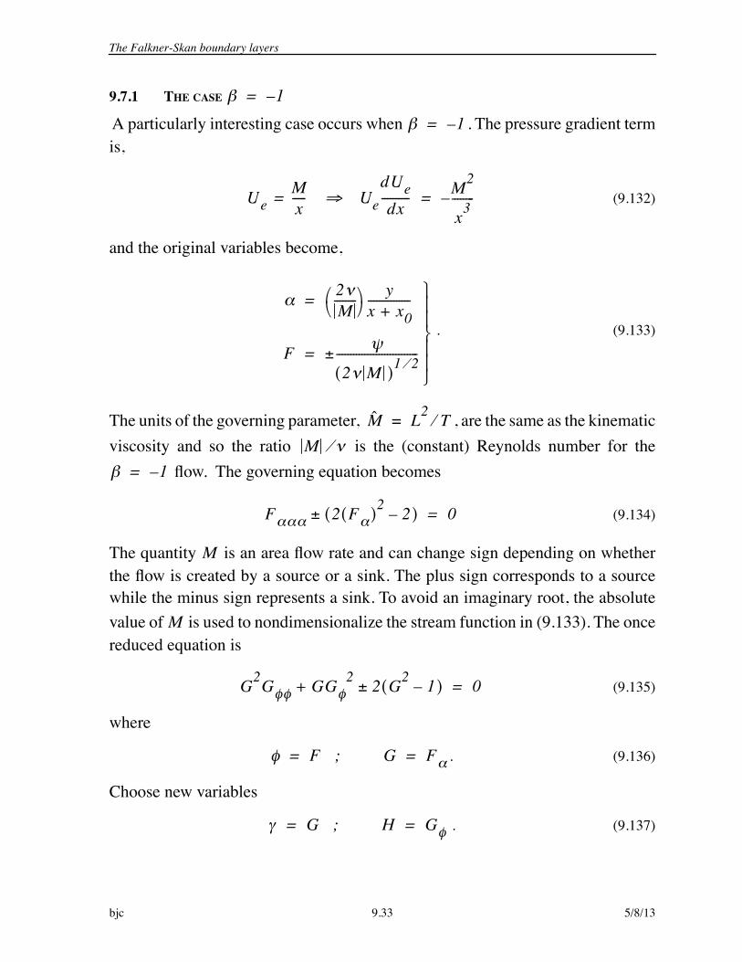
This is shown plotted below.
Figure 9.13 Falkner-Skan sink flow velocity profile .
The Falkner-Skan sink flow represents one of the few known exact solutions ofthe boundary layer equations. However the fact that an exact solution exists forthe case is no accident. Neither is the fact that this case corresponds toan independent variable of the form where both coordinate directionsare in some sense equivalent. Remember the essence of the boundary layerapproximation was that the streamwise direction was in a sense “convective”while the transverse direction was regarded as “diffusive” producing a flow thatis progressively more slender in the direction as increases. In the case of theFalkner-Skan sink flow the aspect ratio of the flow is constant.
9.8 THWAITES’ METHOD FOR APPROXIMATE CALCULATION OF BOUNDARY LAYER CHARACTERISTICS
At the wall the momentum equation reduces to
(9.151)
Rewrite (9.82) as
1 2 3 4 50
0.2
0.4
0.6
0.8
1
F
1–=
1–=y x
y x
2U
y2----------y 0=
Ue-------–dUedx
----------=

Thwaites’ method for approximate calculation of boundary layer characteristics
5/8/13 9.38 bjc
(9.152)
Choose and as length and velocity scales to non-dimensionalize the left
sides of (9.151) and (9.152).
(9.153)
In a landmark paper in 1948 Bryan Thwaites argued that the normalized deriva-tives on the left of (9.153) should depend only on the shape of the velocity profileand not explicitly on the free stream velocity or thickness. Morover he argued thatthere should be a universal function relating the two. He defined
. (9.154)
In terms of the Von Karman equation is
(9.155)
where (9.151) has been used. Thwaites proceeded to examine a variety of knownexact and approximate solutions of the boundary layer equations with a pressuregradient. The main results are shown below.
Uy
-------y 0=
2 H+( )Ue-------
dUedx
----------Ue
2
-------ddx------+=
Ue
2
Ue-------
2U
y2----------
y 0=
2-----–
dUedx
----------=
Ue------- U
y-------
y 0=
2 H+( )2
-----dUedx
----------Ue2-------d 2
dx---------+=
m2
Ue-------
2U
y2----------
y 0=
= l m( ) Ue------- U
y-------
y 0=
=
m
Ue-------d 2
dx--------- 2 2 H+( )m l m( )+( ) L m( )= =

Thwaites’ method for approximate calculation of boundary layer characteristics
bjc 9.39 5/8/13
Figure 9.14 Data collected by Thwaites on skin friction, , shape factor and for a variety of boundary layer solutions.
l m( )
H m( ) L m( )

Thwaites’ method for approximate calculation of boundary layer characteristics
5/8/13 9.40 bjc
The correlation of the data was remarkably good, especially the near straight linebehavior of . Thwaites proposed the linear approximation
(9.156)
One of the classes of solutions included in Thwaites’ data is the Falkner-Skanboundary layers discussed earlier. For these solutions the Thwaites functions canbe calculated explicitly.
(9.157)
The various measures of the Falkner-Skan solutions shown in Figure 9.10 can berelated to instead of using the first equation in (9.157). The relation between
and is shown below.
Figure 9.15 The variable defined in (9.154) versus the free stream velocity exponent for Falkner-Skan boundary layers.
L m( )
L m( ) 0.45 6m+=
m F 0( ) F 1 F–( )d0
22 F 1 F–( )d
0
2–= =
l m( ) F 0( ) F 1 F–( )d0
=
H m( )
1 F–( )d0
F 1 F–( )d0
--------------------------------------------=
mm
m

Thwaites’ method for approximate calculation of boundary layer characteristics
bjc 9.41 5/8/13
The functions and for the Falkner-Skan boundary layer solutions areshown below.
Figure 9.16 Thwaites functions for the Falkner-Skan solutions (9.157).
Thwaites’ correlations were re-examined by N. Curle who came up with a verysimilar set of functions but with slightly improved prediction of boundary layerevolution in adverse pressure gradients. The figures below provide a comparisonbetween the two methods.
Figure 9.17 Comparison between Curle’s functions and Thwaites’ functions.Curle’s tabulation of his functions for Thwaites method is included below.
l m( ) H m( )

Thwaites’ method for approximate calculation of boundary layer characteristics
5/8/13 9.42 bjc
Figure 9.18 Curle’s functions for Thwaites’ method.
A reasonable linear approximation to the data for in Figure 9.17 is
. (9.158)
Equation (9.158) is not the best linear approximation to Curle’s data in Figure9.18 but is consistent with the value of the friction coefficient for the zero-pressure
gradient Blasius boundary layer( ). Insert (9.158) into (9.155)and use the definition of in (9.153) and (9.154).
(9.159)
Equation (9.159) can be integrated exactly.
(9.160)
Equation (9.60) provides the momentum thickness of the boundary layer directlyfrom the distribution of velocity outside the boundary layer . Although the
von Karman integral equation (9.155) was used to generate the data for Thwaites’method, it is no longer needed once (9.160) is known.
L m( )
L m( ) 0.441 6m+=
0.441 0.664=m
Ueddx------
2----- 0.441 6–
2-----
dUedx
----------=
2 0.441
Ue x( )6
------------------ Ue x'( )5 x'd
0
x=
Ue x( )

Thwaites’ method for approximate calculation of boundary layer characteristics
bjc 9.43 5/8/13
The procedure for applying Thwaites’ method is as follows.
1) Given , use (9.160) to determine .
At a given :
2) The parameter is determined from (9.154) and (9.151).
(9.161)
3) The functions and are determined from the data in Figure 9.18.
4)The friction coefficient is determined from
. (9.162)
5) The displacement thickness is determined from .
The process is repeated while progressing along the wall to increasing values of. Separation of the boundary layer is assumed to have occurred if a point is
reached where .
The key references used in this section are
1) Thwaites, B. 1948 Approximate calculations of the laminar boundary layer, VIIInternational Congress of Applied Mechanics, London. Also Aeronautical Quar-terly Vol. 1, page 245, 1949.
2) Curle, N. 1962 The Laminar Boundary Layer Equations, Clarendon Press.
9.8.1 EXAMPLE - FREE STREAM VELOCITY FROM POTENTIAL FLOW OVER A CIRCULARCYLINDER.To illustrate the application of Thwaites’ method let’s see what it predicts for theflow over a circular cylinder where we take as the free stream velocity the poten-tial flow solution.
(9.163)
Ue x( )2 x( )
x
m
m2
-----dUedx
----------–=
l m( ) H m( )
C f2
Ue----------l m( )=
* m( ) H m( )
xl m( ) 0=
UeU-------- 2Sin x
R---=

Thwaites’ method for approximate calculation of boundary layer characteristics
5/8/13 9.44 bjc
Figure 9.19 Example for Thwaites’ method.
According to (9.160)
(9.164)
where
(9.165)
Near the forward stagnation point
(9.166)
Interestingly the method gives a finite momentum thickness at the stagnationpoint. This is useful to know when we apply the method to an airfoil where theradius of the leading adge at the forward stagnation point will define the initialthickness for the boundary layer calculation. Next the relationship between and
is determined using (9.161).
(9.167)
R---
2Re
0.441
Sin6( )
------------------- Sin5 '( ) 'd0
=
ReU 2R----------------=
R---
2Re0
lim 0.4416
------------- 5 'd0
0.4416
-------------= =
m
m2
-----dUedx
----------– 12---
R---–
2Re
dd------
UeU-------- 0.441Cos( )
Sin6( )
--------------------------------– Sin5 '( ) 'd0
= = =
Thwaites’ method for approximate calculation of boundary layer characteristics
bjc 9.45 5/8/13
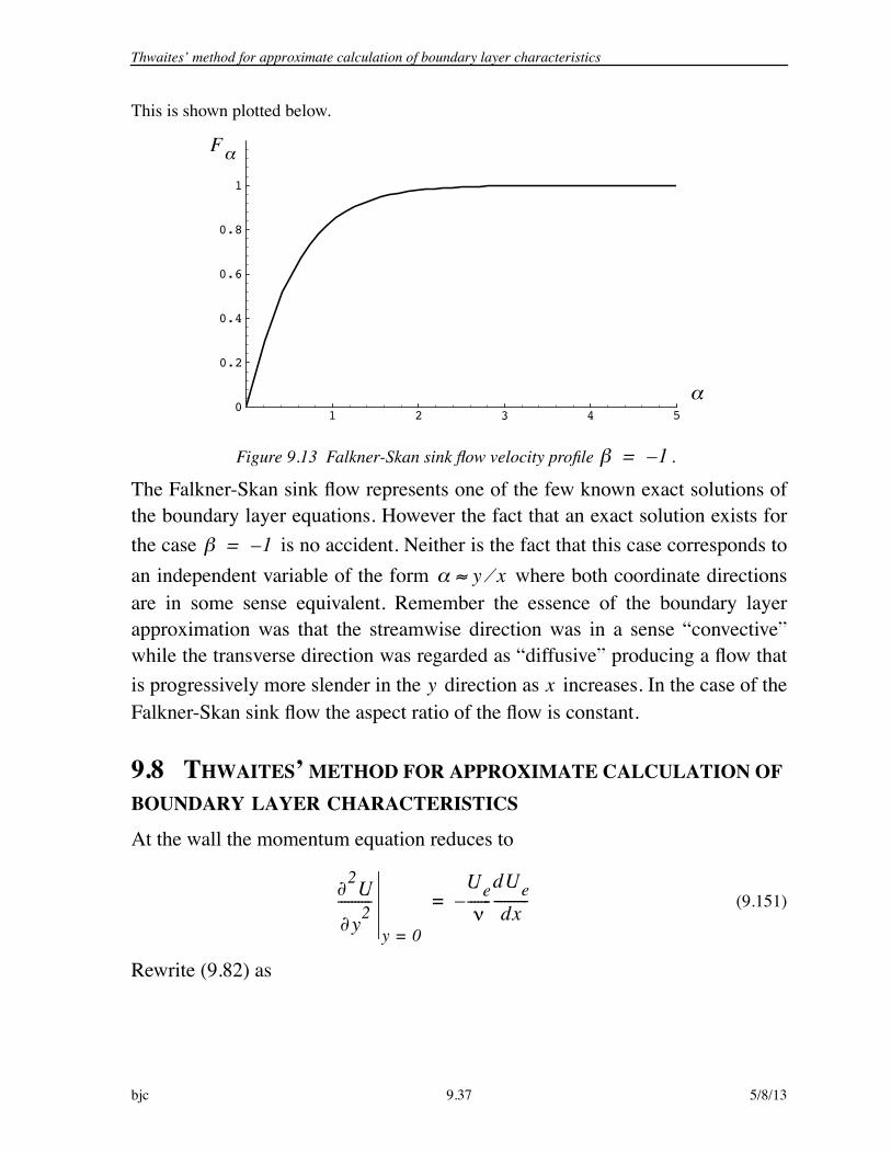
Once is known, is determined from the data in Figure 9.18.
Figure 9.20 Thwaites’ functions for the freestream distribution (9.163).
The friction coefficient determined using (9.162) is shown below.
Figure 9.21 Friction coefficient for the freestream distribution (9.163).
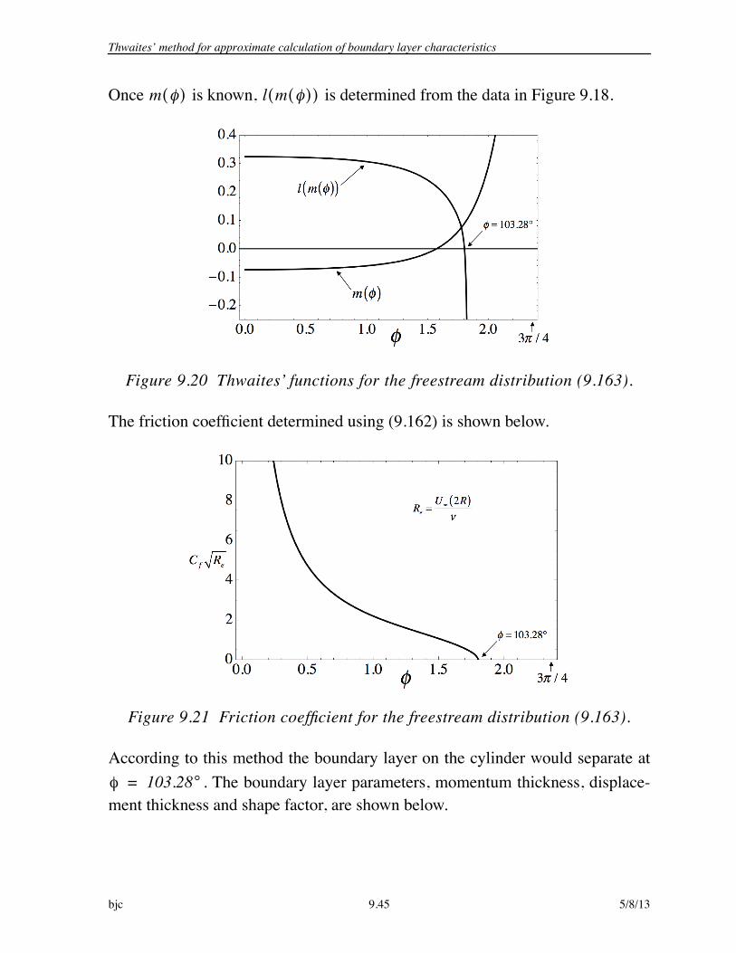
According to this method the boundary layer on the cylinder would separate at. The boundary layer parameters, momentum thickness, displace-
ment thickness and shape factor, are shown below.
m( ) l m( )( )
103.28°=
Compressible laminar boundary layers
5/8/13 9.46 bjc
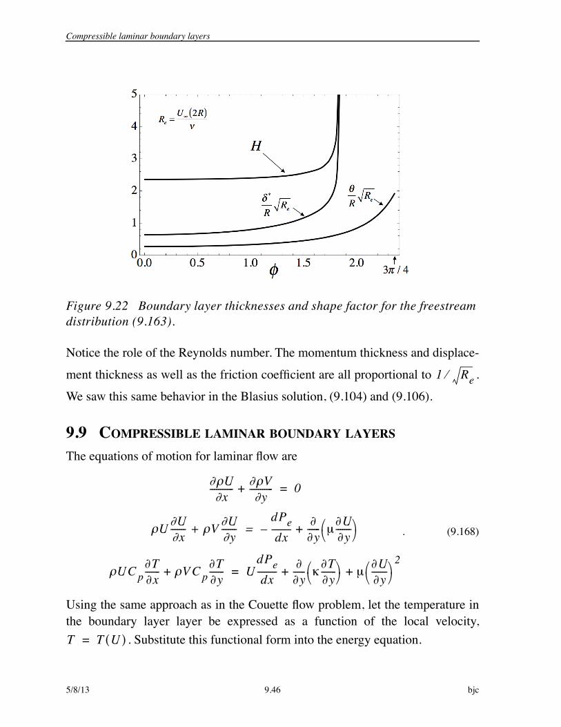
Figure 9.22 Boundary layer thicknesses and shape factor for the freestream distribution (9.163).
Notice the role of the Reynolds number. The momentum thickness and displace-
ment thickness as well as the friction coefficient are all proportional to .
We saw this same behavior in the Blasius solution, (9.104) and (9.106).
9.9 COMPRESSIBLE LAMINAR BOUNDARY LAYERS
The equations of motion for laminar flow are
. (9.168)
Using the same approach as in the Couette flow problem, let the temperature inthe boundary layer layer be expressed as a function of the local velocity,
. Substitute this functional form into the energy equation.
1 Re
Ux
----------- Vy
-----------+ 0=
U Ux
------- V Uy
-------+dPedx
---------– y------ µ
Uy
-------+=
UC pTx
------- V C pTy
-------+ UdPedx
---------y
------ Ty
------- µUy
-------2
+ +=
T T U( )=

Compressible laminar boundary layers
bjc 9.47 5/8/13
(9.169)
Use the momentum equation to replace the factor in parentheses on the left handside of (9.169).
(9.170)
which we can write as
. (9.171)
Introduce the Prandtl number (9.13) which can be assumed to be constant inde-pendent of position in the boundary layer. The energy equation becomes
. (9.172)
There are several important cases to consider.
9.9.1 ENERGY INTEGRAL FOR A COMPRESSIBLE BOUNDARY LAYER WITH AN ADIABATIC
WALL AND
In this case (9.172) reduces to
. (9.173)
The flow at the wall satisfies
. (9.174)
U Ux
------- V Uy
-------+ C pdTdU------- U dP
dx-------
y------ dT
dU------- U
y------- µ
Uy
-------2
+ +=
dPdx-------– y
------ µUy
-------+ C pdTdU-------- U P
x------- dT
dU--------
y------ U
y------- d2T
dU2---------- U
y-------
2µ
Uy
-------2
+ + +=
dPdx-------– C p
dTdU-------- U+ C p
dTdU--------
y------ µ
kC p-------– U
y------- d2T
dU2---------- µ+ U
y-------
2+ + 0=
dPdx-------– C p
dTdU-------- U+ dT
dU--------
Pr 1–Pr
---------------y
------ µUy
------- d2T
dU2---------- µ+ U
y-------
2+ + 0=
Pr 1=
dPdx-------– C p
dTdU------- U+ d2T
dU2---------- µ+ Uy
-------2
+ 0=
U y 0= 0= dTdy-------
y 0=
dTdU------- U
y-------
y 0=0= =
Compressible laminar boundary layers
5/8/13 9.48 bjc
The velocity gradient at the wall is finite as is the wall shear stress so the second condition in (9.174) implies that
. The pressure gradient along the wall is not necessarily zero
so flow conditions at the edge of the boundary layer can vary with the streamwisecoordinate. The temperature must satisfy
(9.175)
and
. (9.176)
Both (9.175) and (9.176) are consistent with the definition of the Prandtl numberand the assumption and integrate to
(9.177)
where is the adiabatic wall temperature defined in (9.20). This temperature
can be expressed in terms of the temperature and velocity at the edge of the bound-ary layer.
(9.178)
Introduce the Mach number at the boundary layer edge . Now
. (9.179)
For a Prandtl number of one the stagnation temperature is constant through theboundary layer at the value at the boundary layer edge.
U y( )y 0= 0
dT dU( )y 0= 0=
d2T
dU2---------- µ---–=
dTdU------- U
C p-------–=
Pr 1=
T wa T– 12C p----------U2=
T wa
T wa T e1
2C p----------Ue
2+=
Me Ue ae=
T waT e
---------- 1 1–2
------------ Me2+
T teT e--------= =
Compressible laminar boundary layers
bjc 9.49 5/8/13
9.9.2 NON-ADIABATIC WALL WITH , AND
Again, although for different reasons than in the previous section, the temperatureis governed by
. (9.180)
In this case, the temperature profile across the boundary layer is
. (9.181)
where is the temperature at the no-slip wall. The heat transfer rate at the wall is
. (9.182)
Thus
. (9.183)
The temperature profile with heat transfer is
(9.184)
which is identical to the temperature profile (9.18) derived for the Couette flowcase for . Evaluate (9.184) at the edge of the boundary layer where the
velocity and temperature and are the same as the free stream values
and . The result is
. (9.185)
The Stanton number was defined in the previous section on Couette flow
dP dx 0= Pr 1=
d2T
dU2---------- µ---–=
C p T T w–( )12---U2+ C p
dTdU-------
y 0=U=
T w
QwTy
-------y 0=
– dTdU-------- U
y-------
y 0=–
µ--- µ
Uy
-------y 0=
dTdU--------
y 0=–= = =
C pdTdU-------
y 0=
C pµ-----------–Qw
w--------=
C p T T w–( )12---U2+
Qw
w--------U–=
Pr 1=
Ue T e U
T
T w T 12C p----------U 2 Qw
wC p--------------U+ +=

Mapping a compressible to an incompressible boundary layer
5/8/13 9.50 bjc
. (9.186)
The adiabatic wall temperature is the free stream stagnation temperature. Using(9.185) in (9.186) gives the friction coefficient in terms of the Stanton number.
(9.187)
which can be compared with the Couette flow result (9.29).
Using (9.184) and (9.185) the temperature profile can be expressed in terms of thefree stream and wall temperatures as follows.
(9.188)
9.10 MAPPING A COMPRESSIBLE TO AN INCOMPRESSIBLE BOUNDARY LAYER
In the late 1940’s L. Howarth (Proc. R. Soc. London A 194, 16-42, 1948) and K.Stewartson (Proc. R. Soc. London A 200, 84-100, 1949) introduced a remarkabletransformation that can be used to map the compressible boundary layer equationsto the incompressible form including the effects of free stream velocity variation.The basic idea is to define a stream function for a virtual incompressible flow thatcarries the same mass flow, integrated to the wall, as the real compressible flow.
Figure 9.23 illustrates the idea. To satisfy the mass balance requirement, the con-stant density of the virtual flow is taken to be the stagnation density of the realflow at the edge of the boundary layer.
(9.189)
The flow at the edge of the boundary layer is assumed to be isentropic
(9.190)
StQw
U C p T w T wa–( )-----------------------------------------------------=
C f 2St=
T T w–T
----------------- 1T wT-------– U
U--------
U2
2C pT------------------ U
U-------- 1 U
U--------–+=
t e 1 1–2
------------ Me2+
1 1–( )=
PtPe------
T tT e------
1–( ) atae-----
2( ) 1–( )
= =

Mapping a compressible to an incompressible boundary layer
bjc 9.51 5/8/13
The pressure through the boundary layer is constant, and .
Figure 9.23 Mapping of a compressible flow to an incompressible flow.
Sutherland’s law is referred to the stagnation temperature of the compressible
flow at the edge of the boundary layer.
(9.191)
The viscosity of the virtual flow, , is the viscosity of the gas evaluated at .
The key assumption needed to make the mapping work is that the viscosity of thegas is linearly proportional to temperature.
(9.192)
where the constant is chosen to provide the best approximation of (9.191).
(9.193)
P Pe= P Pe=
U(y)
x
y
w
Ue(x), Te(x), Pe(x)
(y)
y
x˜
˜w
U y( )
Ue x( ) , Pe x( )
µt
t
Real compressible flow Virtual incompressible flow
µ T
U yd0
y
tU yd0
y=
T t
µµt----- T
T t-----
3 2 T t T S+T T S+-------------------=
µt T t
µµt----- T
T t-----=
T wT t-------
1 2 T t T S+T w T S+---------------------=
Mapping a compressible to an incompressible boundary layer
5/8/13 9.52 bjc
If then . The continuity and momentum equations governing the
compressible flow are
(9.194)
where it is understood that refers to the turbulent shearing stress.
The coordinates of the virtual flow are defined as
. (9.195)
Note that is a function of and since the density depends on both spatialvariables. The variables and are dummy variables of integration. From thefundamental theorem of calculus the derivatives of the coodinates are
. (9.196)
Each of the derivatives is known explicitly except . However, as we willsee in the analysis to follow, terms that involve this derivative will cancel.
Pr 1= 1=
Ux
----------- Vy
-----------+ 0=
U Ux
------- V Uy
-------+ 1---dPedx
---------– 1---y
------ µUy
------- 1--- xyy
-----------+ +=
xy
xPePt------
aeat----- x'd
0
xf x( )= =
yaeat----- x y',( )
t------------------ y'd
0
yg x y,( )= =
y x yx' y'
xx
------ f xPePt------
aeat-----= =
xy
------ f y 0= =
yx
------ gx=
yy
------ gyaeat-----
t-----= =
y x

Mapping a compressible to an incompressible boundary layer
bjc 9.53 5/8/13
The continuity equation is satisfied identically through the introduction of a com-pressible stream function. Let
(9.197)
The stream function of the virtual incompressible flow is a function of and and has the same value as its counterpart in the real compressible flow
since there is the same mass flow between the streamline and the wall in the twoflows.
(9.198)
The mapping we are about to carry out is a bit complicated. In the discussionbelow I have tried to retain as much detail as possible to help the reader getthrough the derivation without requiring a lot of side work to see how one relationfollows from another. Maybe there is more detail than needed but I decided to erron the side of more rather than less to try to give maximum help to the reader.
According to the chain the partial derivatives of in (9.197) are
(9.199)
The velocities can be expressed in terms of the new coodinates as.
(9.200)
The streamwise velocity in the virtual flow is . The mass flowbetween the streamline and the wall in the two flows is depicted in Figure 9.23.
(9.201)
U t y-------= V – t x
-------=
x x( )
y x y,( )
x y,( ) ˜ x x( ) y x y,( ),( )=
x-------
˜x
------- xx
------˜y
------- yx
------+˜x
-------d xdx------
˜y
------- yx
------+= =
y-------
˜x
------- xy
------˜y
------- yy
------+˜y
------- yy
------= =
U t-----y
-------aeat-----
˜y
-------aeat----- U= = =
V t-----– x------- t-----–
PePt------
aeat-----
˜x
------- t-----˜y
------- yx
------–= =
U ˜ y=
U yd0
y
tU yd0
y=

Mapping a compressible to an incompressible boundary layer
5/8/13 9.54 bjc
Differentiate (9.201) at a fixed and use (9.200). The result is
(9.202)
which is consistent with the partial derivative in (9.196). Equation (9.202)confirms that the definition of defined in (9.195) insures that the streamline val-ues in the two flows are the same, that (9.198) holds.
Use the chain rule to determine the first derivatives of that appear in (9.194).
(9.203)
Now we can form the convective terms in (9.194).
(9.204)
Note the terms involving cancel in (9.204). Thus
x
d ydy------ U
tU----------
aeat-----
t-----= =
y y
y
U
Ux
------- x------
aeat-----
˜y
------- d xdx------
y------
aeat-----
˜y
------- yx
------+ = =
PePt------
aeat-----
21ae-----
aex
--------˜y
-------2 ˜x y
------------+aeat-----
2 ˜
y2---------- y
x------+
Uy
------- x------
aeat-----
˜y
------- xy
------y
------aeat-----
˜y
------- yy
------+aeat-----
2
t-----
2 ˜
y2----------= =
U Ux
------- V Uy
-------+ =
PePt------
aeat-----
31ae-----
aex
--------˜y
-------2 ˜
y-------
2 ˜x y
------------+aeat-----
2 ˜y
-------2 ˜
y2---------- y
x------ –+
( )PePt------
aeat-----
aeat-----
2 2 ˜
y2----------
˜x
-------aeat-----
2 2 ˜
y2----------
˜y
------- yx
------+
y x

Mapping a compressible to an incompressible boundary layer
bjc 9.55 5/8/13
(9.205)
Now consider the pressure gradient term. Assume the flow at the edge of theboundary layer is isentropic.
(9.206)
The pressure gradient term can be expressed in terms of the speed of sound at theboundary layer edge.
(9.207)
Now
. (9.208)
Note that, from (9.200)
U Ux
------- V Uy
-------+ =
PePt------
aeat-----
31ae-----
aex
--------˜y
-------2 ˜
y-------
2 ˜x y
------------2 ˜
y2----------
˜x
-------–+
PePt------
aeat-----
21–( )
-----------------
=
dPedx
---------2 Pt
1–( )-----------------
aeat-----
1+1–
-------------1at----
daed x---------d x
dx------
PePt------
aeat-----
2 Pt1–( )
-----------------aeat-----
1+1–
-------------1at----
daed x---------= =
dPedx
---------PePt------
aeat-----
2 2 Pt1–( )
-----------------aeat-----
1+1–
-------------1ae-----
daed x---------=
U Ux
------- V Uy
------- 1---dPedx
---------+ + =
PePt------
aeat-----
3 ˜y
-------2 ˜x y
------------2 ˜
y2----------
˜x
-------– +
PePt------
aeat-----
3 ˜y
-------2 1---
2 Pt1–( )
-----------------aeat-----
21–
------------
+ 1ae-----
daed x---------
Mapping a compressible to an incompressible boundary layer
5/8/13 9.56 bjc
. (9.209)
So far
. (9.210)
The flow at the edge of the boundary layer is adiabatic.
(9.211)
and
(9.212)
Now
. (9.213)
˜y
-------2
U2 atae-----
2=
U Ux
------- V Uy
------- 1---dPedx
---------+ + =
PePt------
aeat-----
3 ˜y
-------2 ˜x y
------------2 ˜
y2----------˜x
-------– +
PePt------
aeat-----
3U2 at
ae-----
21---
2 Pt1–( )
-----------------aeat-----
21–
------------
+ 1ae-----
daed x---------
at2 ae
2 1–2
------------ Ue2+=
1ae-----
daed x--------- 1–
2ae2------------ Ue
dUed x
----------–=
U Ux
------- V Uy
------- 1---dPedx
---------+ + =
PePt------
aeat-----
3 ˜y
-------2 ˜x y
------------2 ˜
y2----------˜x
-------– –
PePt------
aeat-----
3U2 1–( )
2ae2-----------------
atae-----
21---
Pt
ae2--------
aeat-----
21–
------------
+ UedUed x
----------

Mapping a compressible to an incompressible boundary layer
bjc 9.57 5/8/13
Note that
(9.214)
where we have used the isentropic relation and
. Now work out the viscous term using
.
(9.215)
Recall and . The viscous stress term in
the boundary layer equation is
. (9.216)
The turbulent stress term transforms as
. (9.217)
U2 1–( )
2ae2-----------------
atae-----
21---
Pt
ae2--------
aeat-----
21–
------------
+ =
U2 1–( )
2ae2-----------------
atae-----
2e-----
Pe
e--------- 1
ae2-----
atae-----
21–
------------aeat-----
21–
------------
+ =
atae-----
4 a2 1–( )2
-----------------U2+
at2-------------------------------------
Pt Pe at ae( )2 1–( )=
Pe P( ) a2= =
T P R Pe R= =
xy laminarµ
Uy
------- µtTT t-----
y------
aeat-----
˜y
------- µtTT t-----
aeat-----
y------
˜y
------- = = = =
µtaeat-----
2TT t-----
t-----
y------
˜y
-------aeat-----
2T
tT t----------- µt
Uy
-------aeat-----
2 PePt------ ˜ x y laminar
= =
U ˜ y= ˜ x y laminarµt U y=
1---y
------ µUy
-------µt
t-----
PePt------
aeat-----
3 3 ˜
y3----------=
˜ xy turbulent
1---atae-----
2 PtPe------ xy turbulent
=

Mapping a compressible to an incompressible boundary layer
5/8/13 9.58 bjc
which can be expressed as
. (9.218)
Now the boundary layer momentum equation (9.194)becomes
. (9.219)
Drop the common factor multiplying each term on the right of (9.219). The trans-formed equation is nearly in incompressible form.
(9.220)
The real and virtual free stream velocities are related by
. (9.221)
which comes from the expression for in (9.200). Differentiate (9.221)
1---y
------ xy turbulent
1t
-----PePt------
aeat-----
3
y------ ˜ xy turbulent
=
U Ux
------- V Uy
------- 1---dPedx
--------- 1---y
------ µUy
-------– 1--- xyy
-----------–+ + =
PePt------
aeat-----
3 ˜y
-------2 ˜x y
------------2 ˜
y2----------
˜x
-------– –
PePt------
aeat-----
3 atae-----
4 a2 1–( )2
-----------------U2+
at2
-------------------------------------- UedUed x
---------- –
µt
t-----
PePt------
aeat-----
3 3 ˜
y3---------- 1
t-----
PePt------
aeat-----
3
y------ ˜ xy turbulent
– 0=
˜y
-------2 ˜x y
------------2 ˜
y2----------
˜x
-------–atae-----
4 a2 1–( )2
-----------------U2+
at2
--------------------------------------- UedUed x
---------- ––
µt
t-----
3 ˜
y3---------- 1
t-----
y------ ˜ xy turbulent( )– 0=
Ueatae-----Ue=
U
Mapping a compressible to an incompressible boundary layer
bjc 9.59 5/8/13
(9.222)
and substitute (9.222) into (9.220).
. (9.223)
The velocities in the virtual flow are
. (9.224)
The transformed boundary layer momentum equation finally becomes
. (9.225)
For an adiabatic wall and the factor in brackets is equal to one. In this
case the momentum equation maps exactly to the incompressible form.
(9.226)
with boundary conditions
UedUed x
----------atae-----
21
ae2
----- ae2 1–
2------------ Ue
2+ UedUed x
---------- = =
atae-----
4Ue
dUed x
----------
˜y
-------2 ˜x y
------------2 ˜
y2----------
˜x
-------–a2 1–( )
2-----------------U2+
at2
-------------------------------------- UedUed x
---------- ––
µt
t-----
3 ˜
y3---------- 1
t-----
y------ ˜ xy turbulent
– 0=
U˜y
-------= V˜x
-------–=
U Ux
------- Uy
------- V+a2 1–( )
2-----------------U2+
ae2 1–( )
2-----------------Ue
2+------------------------------------------- Ue
dUed x
---------- ––
t
2U
y2---------- 1
t-----
y------ ˜ xy turbulent
–
Pr 1=
U Ux
------- Uy
------- V+ UedUed x
---------- t
2U
y2----------– 1
t-----
y------ ˜ xy turbulent
–– 0=

Mapping a compressible to an incompressible boundary layer
5/8/13 9.60 bjc
(9.227)
The implication of (9.226) and (9.227) is that the effects of compressibility on theboundary layer can be almost completely accounted for by the scaling of coordi-nates presented in (9.195) which is driven in the direction by the decrease indensity near the wall due to heating and in the direction by the isentropicchanges in free stream temperature and boundary layer pressure due to flow accel-eration or deceleration imposed by the surrounding potential flow.
Let’s use this transformation to relate the skin friction in the compressible case tothe incompressible skin friction. The definition of the friction coefficient is
(9.228)
Recall that for the constant . In terms of the Mach number, the
ratio of friction coefficients in the real compressible flow and the virtual incom-pressible flow is
. (9.229)
The physical velocity profiles in the compressible flow cannot be determinedwithout solving for the temperature in the boundary layer. Here we will restrictour attention to the laminar, zero pressure gradient, Blasius case, ,
. The temperature equation was integrated earlier to give
. (9.230)
Equation (9.230) can be expressed as
U 0( ) 0= V 0( ) 0= U ˜( ) Ue=
yx
C f˜w
1 2( ) tUe2
----------------------------
1---atae-----
2 PtPe------ w
1 2( ) t
e----- e
atae-----
2Ue
2-------------------------------------------------------- 1---
ePt
tPe----------- w
1 2( ) eUe2
----------------------------- 1---T tT e------C f= = = =
Pr 1= 1=
C fC f------- 1
1 1–2
------------ Me2+
------------------------------------=
dUe dx 0=
xy turbulent0=
T T t1
2C p----------U2–=

Mapping a compressible to an incompressible boundary layer
bjc 9.61 5/8/13
. (9.231)
Using the first relation in (9.18) , and the equality ,
equation (9.231) becomes
. (9.232)
Our goal is to relate the wall normal coordinate in compressible and incompress-ible flows. From (9.196)
(9.233)
The spatial similarity variable in the virtual flow is
(9.234)
Now (9.233) becomes
(9.235)
and
(9.236)
Rearrange the coefficient on the right hand side of (9.236) using (9.195) and(9.200).
TT e------ 1 1–
2------------ Me
2 1 UUe-------
2–+=
U Ue U Ue= T eT e=
TT e------ 1 1–
2------------ Me
2 1 UUe-------
2–+ e-----= =
dyatae----- t
e----- e----- d y
atae----- t
e----- 1 1–
2------------ Me
2 1 UUe-------
2–+ dy= =
˜ yUe
2 t x-----------
1 2=
dyatae----- t
e-----
2 t x
Ue-----------
1 21 1–
2------------ Me
2 1 UUe-------
2–+ d y
Ue2 t x-----------
1 2=
d yUe
2 ex------------
1 2 =
atae----- t
e-----
2 t x
Ue-----------
1 2 Ue2 ex------------
1 21 1–
2------------ Me
2 1 UUe-------
2–+ d y
Ue2 t x-----------
1 2
Mapping a compressible to an incompressible boundary layer
5/8/13 9.62 bjc
(9.237)
Finally.
(9.238)
Integrate (9.238). The similarity variables in the real and virtual flows are relatedby
(9.239)
The velocity ratio, is a known function from the Blasius solution.
The outer edge of the incompressible boundary layer is at
. The integral of the velocity term in (9.239) is
. (9.240)
This allows us to determine how the thickness of the compressible layer dependson Mach number. The outer edge of the compressible boundary layer is at
. (9.241)
The thickness of the compressible layer grows rapidly with Mach number. Know-ing enables the temperature and density of the compressible layer to bedetermined.
atae----- t
e-----
2 t x
Ue-----------
Ue2 ex------------
1 2 atae----- t
e-----
µtµe----- e
t-----
Ue
Ue------- x
x--
1 2 = =
atae----- t
e-----
T tT e------ e
t-----
aeat-----
PePt------
aeat-----
1 2t
e-----
T tT e------ e
t----- eT e
tT t------------
1 21= =
d 1 1–2
------------ Me2 1 U
Ue-------
2–+ d ˜=
˜( ) ˜ 1–2
------------ Me2 1 U
Ue-------
2– d '˜
0
˜+=
U Ue F ˜ ˜( )
˜ e 4.906 2 3.469= =
1 UUe-------
2– ˜d
0
˜ e1.67912=
e ˜ e1–
2------------ Me
2 1 UUe-------
2– ˜d
0
˜ e+ = =
e 3.469 1.67912 1–2
------------ Me2+=
˜( )

Turbulent boundary layers
bjc 9.63 5/8/13
(9.242)
Numerically determined solutions for the velocity profile at several Mach num-bers are shown below.
Figure 9.24 Compressible boundary layer profiles on an adiabatic plate for , viscosity exponent , and .
The compressible layer is considerably thicker than the incompressible layer dueto the high temperature and low density near the wall caused by the decelerationof the flow.
9.11 TURBULENT BOUNDARY LAYERS
As the Reynolds number increases along the plate a point is reached where thelaminar boundary layer begins to be unstable to small disturbances. A complexseries of events occurs by which the flow becomes turbulent characterized by veryrapid mixing of momentum in the transverse direction. As a result the velocityprofile becomes much fuller and the velocity gradient near the wall becomes muchsteeper compared to the velocity gradient that would have occurred if the layerhad remained laminar. The friction at the wall is also correspondingly much largerand the growth rate of the boundary layer is much faster as suggested schemati-cally in Figure 9.25 below.
T ˜( )( )T e
---------------------- e˜( )( )
--------------------- 1 1–2
------------ Me2 1 U ˜( )
Ue-------------
2–+= =
Pr 1= 1= 1.4=
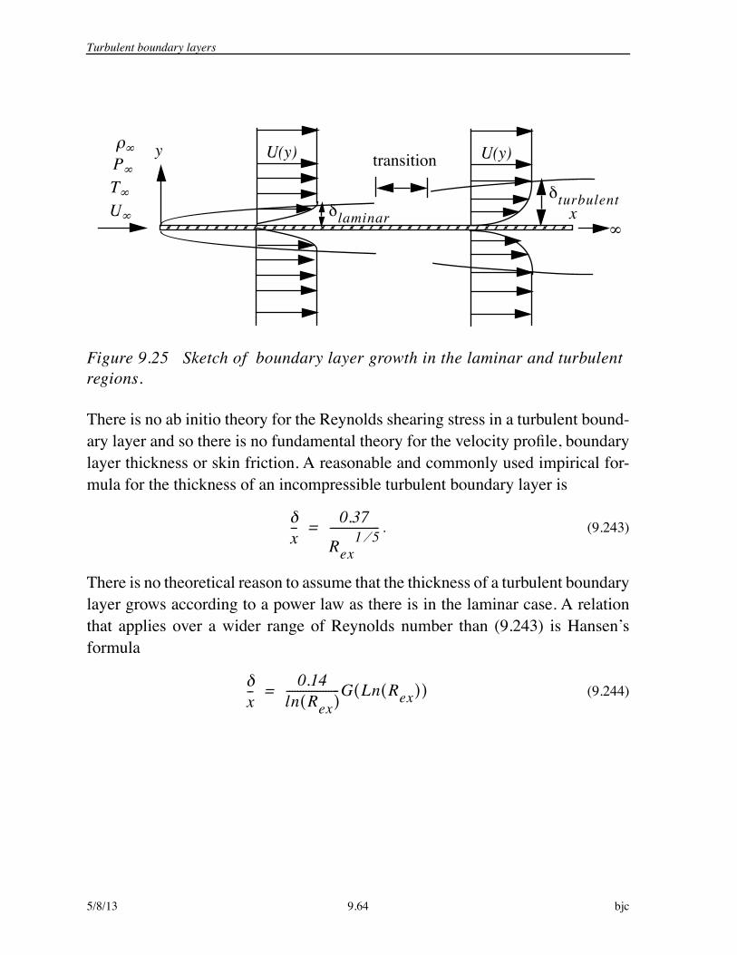
Turbulent boundary layers
5/8/13 9.64 bjc
Figure 9.25 Sketch of boundary layer growth in the laminar and turbulent regions.
There is no ab initio theory for the Reynolds shearing stress in a turbulent bound-ary layer and so there is no fundamental theory for the velocity profile, boundarylayer thickness or skin friction. A reasonable and commonly used impirical for-mula for the thickness of an incompressible turbulent boundary layer is
. (9.243)
There is no theoretical reason to assume that the thickness of a turbulent boundarylayer grows according to a power law as there is in the laminar case. A relationthat applies over a wider range of Reynolds number than (9.243) is Hansen’sformula
(9.244)
U(y)
x
y
UTP U(y)
laminarturbulent
transition
x-- 0.37
Rex1 5
------------------=
x-- 0.14
ln Rex( )-------------------G Ln Rex( )( )=
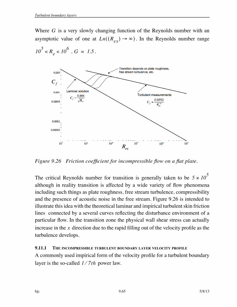
Turbulent boundary layers
bjc 9.65 5/8/13
Where is a very slowly changing function of the Reynolds number with anasymptotic value of one at . In the Reynolds number range
, .
Figure 9.26 Friction coefficient for incompressible flow on a flat plate.
The critical Reynolds number for transition is generally taken to be although in reality transition is affected by a wide variety of flow phenomenaincluding such things as plate roughness, free stream turbulence, compressibilityand the presence of acoustic noise in the free stream. Figure 9.26 is intended toillustrate this idea with the theoretical laminar and impirical turbulent skin frictionlines connected by a several curves reflecting the disturbance environment of aparticular flow. In the transition zone the physical wall shear stress can actuallyincrease in the direction due to the rapid filling out of the velocity profile as theturbulence develops.
9.11.1 THE INCOMPRESSIBLE TURBULENT BOUNDARY LAYER VELOCITY PROFILE
A commonly used impirical form of the velocity profile for a turbulent boundarylayer is the so-called power law.
GLn Rex( )( )
105 Re 106< < G 1.5=
5 105×
x
1 7th

Turbulent boundary layers
5/8/13 9.66 bjc
(9.245)
This profile can be useful in a limited range of Reynolds numbers but it fails tocapture one of the most important features of the turbulent boundary layer whichis that the actual shape of the velocity profile depends on the Reynolds number.In contrast, the Blasius profile shape is completely independent of Reynolds num-ber. Only the thickness changes with Reynolds number.
While there is no good theory for the velocity profile in a turbulent boundary, thereis a very good correlation that accurately reflects certain fundamental flow prop-erties and can be used to analyze and compare flows at different Reynoldsnumbers.
The first thing to know is that the flow near the wall, when properly normalized,has a universal shape that is independent of the parameters that govern the outerflow. The idea is to normalize the velocity near the wall by the so-called frictionvelocity
(9.246)
This leads to the definition of dimensionless wall variables.
(9.247)
The thickness of the boundary layer in wall units is
(9.248)
If we use the impirical formulas for thickness and skin friction described abovethen
(9.249)
and
UUe------- y--
1 7=
u*= w------ w µUy
-------y 0=
=
y+ yu*---------= U+ Uu*------=
+ u*---------=
u*Ue------- w
Ue2
-----------1 2 C f
2-------
1 2 0.0592
2Rex1 5
----------------1 2 0.172
Rex1 10
---------------= = = =

Turbulent boundary layers
bjc 9.67 5/8/13
(9.250)
In other words, once is known most of the important properties of the bound-
ary layer are known. A typical velocity profile is shown below. I have chosen arelatively low Reynolds number so that the flow near the wall can be seen at areasonable scale.
Figure 9.27 Turbulent boundary layer velocity profile in linear and log-lin-
ear coordinates. The Reynolds number is
The boundary layer is generally thought of as comprising several layers and theseare indicated in Figure 9.27. Usually they are delineated in terms of wall variables.
Viscous sublayer - Wall to A, . In this region closest to the wall the vel-city profile is linear.
(9.251)
Buffer layer - A to B, . Several alternative formulations are used toapproximate the velocity in this region. An implicit relation that works reasonablywell all the way to the wall is
(9.252)
+x-- u*
Ue-------
Uex---------- 0.37
Rex1 5
------------------ 0.172
Rex1 10
--------------- Rex 0.0636Rex7 10= = =
Rex
Rex 106=
0 y+ 7<
U + y+=
7 y+ 30<
y+ U + e C– e U+1– U +– 1
2--- U +( )
2– 1
6--- U +( )
3– 1
24------ U +( )
4–+=

Turbulent boundary layers
5/8/13 9.68 bjc
Logarithmic and outer layer - B to C to D . An impirical formulathat works well and includes the effect of pressure gradient is
(9.253)
The slope of the profile in the logarithmic region is inversely proportional to theKarman constant which is generally taken to be and is viewed as auniversal constant of turbulent flows. However modelers of meteorological flowssuch as the atmospheric boundary layer have deduced values of as low as while recent experiments in very high Reynolds number pipe flow at Princetonhave suggested values as high as .
The constant depends on the wall roughness. If is a measure of the height
of roughness elements at the wall one can define as a roughness
Reynolds number. The wall is considered hydraulically smooth if and
hydraulically rough if . For a hydraulically smooth wall in
(9.253) and increases with increasing . The function is determined by
the pressure gradient and layer Reynolds number. For , .
The logarithmic term in (9.253) is remakably robust in the presence of pressuregradients and roughness. The constant hardly changes at all with roughness.
The term in (9.253) is called the wake function because of the vaguely wakelike shape of the outer velocity profile. Something to notice is that the velocity
profile (9.253) is not valid beyond and the velocity profile has a small
but finite slope at because of the logarithmic term.
Figure 9.28 compares turbulent boundary layer profiles at various Reynolds num-bers. The effect of Reynolds number on the flow expressed in wall variables is felt
through the value of in the wake function term in (9.253). In Figure 9.28 thereis a slight mismatch between (9.252) and (9.253) at the outer edge of the buffer
30 y+ +<
U + 1--- y+( ) C 2 x( )------------Sin2
2--- y+
+------+ +ln=
0.4=
0.35
0.436
C ks
Res u*ks =
Res 3<
Res 100> C 5.1=
Res x( )
dPe dx 0= 0.62=
Sin2
y+ +=
y+ +=
+
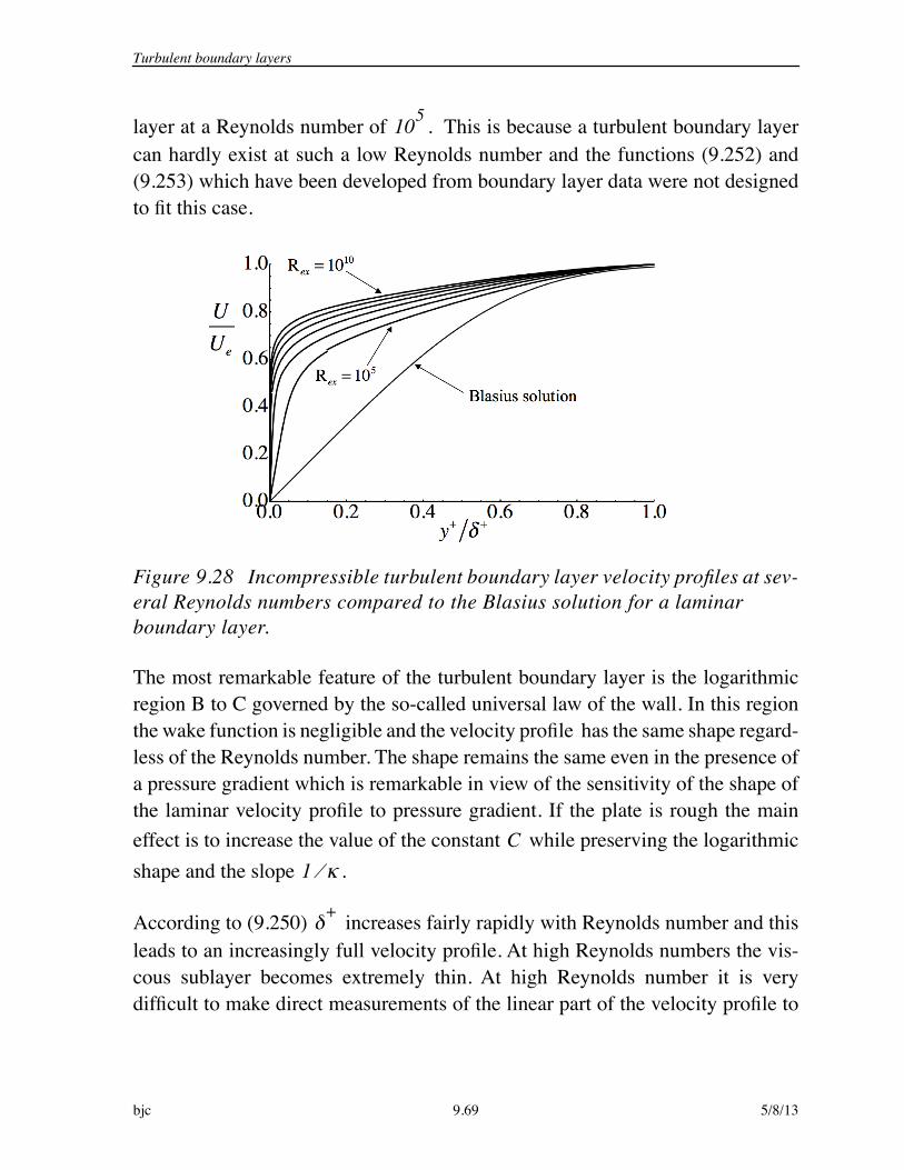
Turbulent boundary layers
bjc 9.69 5/8/13
layer at a Reynolds number of . This is because a turbulent boundary layercan hardly exist at such a low Reynolds number and the functions (9.252) and(9.253) which have been developed from boundary layer data were not designedto fit this case.
Figure 9.28 Incompressible turbulent boundary layer velocity profiles at sev-eral Reynolds numbers compared to the Blasius solution for a laminar boundary layer.
The most remarkable feature of the turbulent boundary layer is the logarithmicregion B to C governed by the so-called universal law of the wall. In this regionthe wake function is negligible and the velocity profile has the same shape regard-less of the Reynolds number. The shape remains the same even in the presence ofa pressure gradient which is remarkable in view of the sensitivity of the shape ofthe laminar velocity profile to pressure gradient. If the plate is rough the maineffect is to increase the value of the constant while preserving the logarithmicshape and the slope .
According to (9.250) increases fairly rapidly with Reynolds number and thisleads to an increasingly full velocity profile. At high Reynolds numbers the vis-cous sublayer becomes extremely thin. At high Reynolds number it is verydifficult to make direct measurements of the linear part of the velocity profile to
105
C1
+

Transformation between flat plate and curved wall boundary layers
5/8/13 9.70 bjc
determine skin friction. Fortunately the skin friction can be determined usingmeasurements in the much more accessible logarithmic region by utilizing the lawof the wall.
(9.254)
Measurements of versus in region B-C can be used to determine andhence . The friction coefficient in the compressible case can be estimated using
(9.229).
9.12 TRANSFORMATION BETWEEN FLAT PLATE AND CURVED WALL BOUNDARY LAYERS
One of the consequences of the boundary layer approximation is that the solutionfor the flow on a flat plate with a variable free stream velocity can be transformeddirectly to the solution on a curved wall with the same free stream velocity func-tion. Once again the boundary layer equations are
(9.255)
where includes both laminar and turbulent components of shearing stress and
includes laminar and turbulent componenst of heat flux. The transformation
of variables between the flat plate and curved wall is.
U
U*------- 1--- yU*---------- C+ln=
U y U*
C f
Ux
----------- Vy
-----------+ 0=
U Ux
------- V Uy
-------dPedx
--------- xyy
-----------–+ + 0=
UC pTx
------- V C pTy
------- UdPedx
---------Qyy
----------+– xyUy
-------–+ 0=
xy
Qy
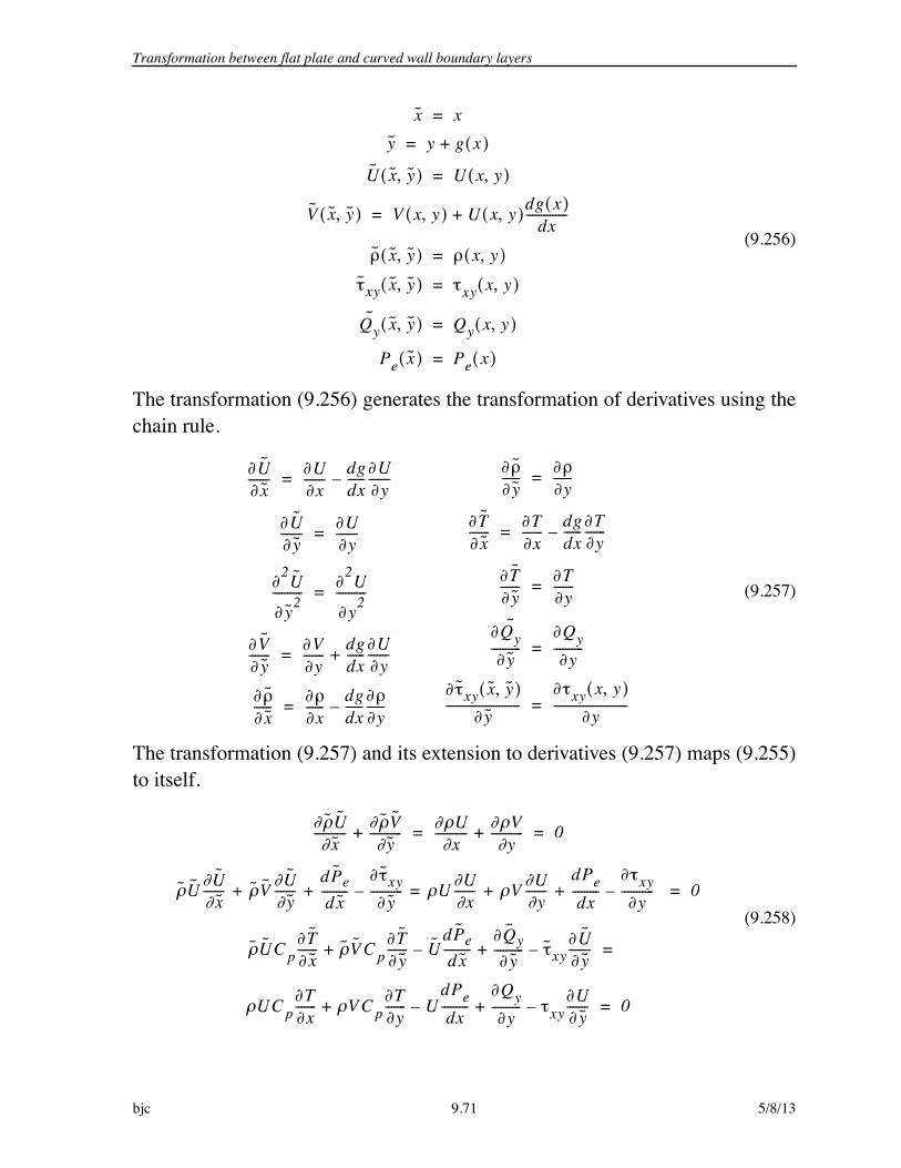
Transformation between flat plate and curved wall boundary layers
bjc 9.71 5/8/13
(9.256)
The transformation (9.256) generates the transformation of derivatives using thechain rule.
(9.257)
The transformation (9.257) and its extension to derivatives (9.257) maps (9.255)to itself.
(9.258)
x x=y y g x( )+=
U x y,( ) U x y,( )=
V x y,( ) V x y,( ) U x y,( )dg x( )
dx--------------+=
˜ x y,( ) x y,( )=˜ xy x y,( ) xy x y,( )=
Qy˜ x y,( ) Qy x y,( )=
Pe x( ) Pe x( )=
Ux
------- Ux
------- dgdx------ U
y-------–=
Uy
------- Uy
-------=
2U
y2----------
2U
y2----------=
Vy
------- Vy
------- dgdx------ U
y-------+=
˜x
------x
------ dgdx------
y------–=
˜y
------y
------=
Tx
------- Tx
------- dgdx------ T
y-------–=
Ty
------- Ty
-------=
Qy˜
y----------
Qyy
----------=
˜ xy x y,( )
y------------------------- xy x y,( )
y-------------------------=
˜ Ux
-----------˜ Vy
-----------+ Ux
----------- Vy
-----------+ 0= =
˜ U Ux
------- ˜ V Uy
-------dPed x
---------˜ xyy
-----------–+ + U Ux
------- V Uy
-------dPedx
--------- xyy
-----------–+ += 0=
˜ UC pTx
------- ˜ V C pTy
------- UdPed x
---------Qyy
----------+– ˜ xyUy
-------–+ =
UC pTx
------- V C pTy
------- UdPedx
---------Qyy
----------+– xyUy
-------–+ 0=

Transformation between flat plate and curved wall boundary layers
5/8/13 9.72 bjc
In principle the function added to the coordinate is arbitrary, but in prac-tice is restricted to be smooth and slowly varying so as not to violate theboundary layer approximation.
It is the absence of the derivative from (9.255) that enables the transfor-mation (9.256) and (9.257) to reproduce the same equations in the newcoordinates. The figure below illustrates the idea.
Figure 9.29 Mapping of the boundary layer developing over an airfoil to the boundary layer on a flat plate with a pressure gradient.
The function defines the surface of the airfoil in the Cartesian coordinates. The flow at a given distance from the leading edge and a distance
above the surface of the airfoil is mapped to the same position in theboundary layer on a flat plate with the same free stream flow velocity
g x( ) yg x( )
V x
g x( )
x y,( ) xy g x( )–

Problems
bjc 9.73 5/8/13
. The main restriction on is that it vary slowly enough so
that the boundary layer does not approach separation and so that the approxima-tion remains valid.
The exponential decay of the vorticity at the edge of the boundary layer describedearlier, together with this simple invariance of the boundary layer equationsenables boundary layer theory to be applied to a wide variety of slender bodyshapes creating one of the most powerful tools in fluid mechanics.
An iterative algorithm can be used to determine the viscous flow over a complexshape such as the airfoil shown in Figure 9.29. The procedure is
1) Solve for the potential flow over the airfoil.
2) Use the potential flow velocity at the airfoil surface as the for a bound-
ary layer calculation beginning at the leading edge.
3) Determine the displacement thickness of the boundary layer and use the datato define a new airfoil shape. Repeat the potential flow calculation using the newairfoil shape to determine a new .
4) Using the new repeat the boundary layer calculation.
A few iterations of this viscous-inviscid interaction procedure will converge to anaccurate solution for the viscous, compressible flow over the airfoil.
9.13 PROBLEMS
Problem 1 - The figure below depicts Couette flow of an ideal gas betweentwo infinite parallel. The lower wall is adiabatic.
Determine the entropy difference between the lower and upper walls.
Ue x( ) Ue x( )= g x( )
x x
Ue x( )
Ue x( )
Ue x( )
TU
y

Problems
5/8/13 9.74 bjc
Problem 2 - The figure below depicts Couette flow of helium gas between twoinfinite parallel walls spaced 1 cm apart. The lower wall is adiabatic and thespeed of the upper wall is 400 meters/sec. The temperature of the upper wallis 300K.
Assume the viscosity depends linearly on temperature.
. (9.259)
Set up and solve the compressible flow equations for this simple flow. Notethat the flow is assumed to be steady and all flow variables depend only on thecoordinate normal to the wall.
1) Determine the speed of sound at the upper wall.
2) Determine the temperature of the lower wall.
3) Determine the shear stress.
4) Is there work done on the flow? How much?
5) Determine the heat flux through the upper wall.
6) Sketch the distribution of stagnation temperature across the channel.
7) Sketch the distribution of entropy across the channel.
UT
µ µ T T=

Problems
bjc 9.75 5/8/13
Problem 3 - The figure below depicts Couette flow of a gas between two infi-nite parallel walls spaced a distance apart. The lower wall is adiabatic. The
reference Mach number is . The viscosity is assumed to
depend linearly on temperature and the reference Reynolds
number is .
Sketch how the friction coefficient depends on . At what Mach numberis the friction coefficient an extremum? Is it a maximum or a minimum?Express your answer in terms of and the Prandtl number. What are the val-ues for helium and air?
Problem 4 - The figure below shows the unsteady flow produced by a flat plateset into motion impulsively at velocity .
The plate extends to infinity in both directions and the flow is perfectly parallel.Simplify the compressible flow equations. Solve for the velocity and vorticity inthe incompressible case.
Problem 5 - In the discussion of boundary layers we defined several defini-tions of the thickness. How would you define a thickness based on the vorticitydistribution? What might be the advantage of such a definition?
d
M U RT=
µ µ T T=
Re U d µ=
TU
C f U
U
Ux
y

Problems
5/8/13 9.76 bjc
Problem 6 - Use the Howarth-Stewartson transformation to generate thevelocity and temperature profiles in a laminar, compressible, zero pressure-gradient boundary layer at a free stream Mach number .M 8=